Energy barriers, entropy barriers, and non-Arrhenius behavior in a minimal glassy model

Abstract

We study glassy dynamics using a simulation of three soft Brownian particles confined to a two-dimensional circular region. If the circular region is large, the disks freely rearrange, but rearrangements are rarer for smaller system sizes. We directly measure a one-dimensional free energy landscape characterizing the dynamics. This landscape has two local minima corresponding to the two distinct disk configurations, separated by a free energy barrier which governs the rearrangement rate. We study several different interaction potentials and demonstrate that the free energy barrier is composed of a potential energy barrier and an entropic barrier. The heights of both of these barriers depend on temperature and system size, demonstrating how non-Arrhenius behavior can arise close to the glass transition.

I Introduction

Glassy materials are amorphous solids: disordered microscopically, and unable to flow macroscopically biroli13 ; ediger12 ; cavagna09 ; dyre06 . They are inherently out of equilibrium angell00 ; cipelletti02 , in contrast to crystals. In 1969, Goldstein proposed the idea of the potential energy landscape, a conceptual framework for thinking about glassy and crystalline materials goldstein69 . The potential energy landscape is defined as the potential energy $U$ of a material “plotted as a function of $3N$ atomic coordinates in a $3N+1$ dimensional space,” where $N$ is the number of atoms goldstein69 . At low temperatures, an ideal crystalline solid will have particle coordinates that correspond to a global minimum of the potential energy landscape. Glasses are disordered, so at low temperatures a glass will have coordinates in a local minimum of the potential energy landscape, but there are an enormous number of such local minima debenedetti01 ; stillinger95 ; sciortino05rev ; heuer08 .

Turning to higher temperatures where a material is a liquid, thermal energy allows the system to rearrange constantly, and so the $3N$ atomic coordinates trace out a trajectory traversing the potential energy landscape. If the temperature is close to the material’s glass transition, and if crystallization is avoided, then the trajectory through the landscape spends most of its time near local minima, with occasional passages through a saddle point in the landscape to an adjacent minimum stillinger82 ; sastry98 . The number of minima, their depth, and the details of the saddles between them can be connected to the microscopic dynamics of samples at a variety of temperatures sciortino05rev ; heuer08 . At low temperatures, the thermal energy $k_{B}T$ does not allow the system to escape a local minimum easily. In particular the escape from any particular local minimum is a thermally activated process, depending on the barrier height between that local minimum and the minima adjacent in the $3N+1$ dimensional space. Of course, given the high dimensionality of the problem, visualizing this is impossible except for conceptual sketches stillinger95 ; perezcastaneda14 ; charbonneau14 , of which the earliest one we are aware of was by Stillinger and Weber in 1984 stillinger84 .

The picture of a potential energy landscape changes when one considers a system of hard spheres. Hard spheres are defined as particles that have no interaction energy when they are not in contact, and infinite interaction energy if they touch. As a function of the $3N$ sphere coordinates, the potential energy surface is flat at $U=0$ except for prohibited configurations for which $U=\infty$. Rather than local minima separated by saddles, the landscape has flat open areas separated by bottlenecks that correspond to entropic barriers. As hard spheres can form glasses at high densities cohen59 ; woodcock81 ; speedy98 , these entropic barriers must function similarly to the potential energy barriers in a potential energy landscape bowles99 ; ashwin09 ; hunter12pre .

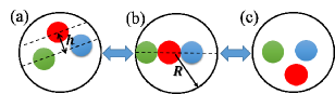
Figure 1: (Color online) Sketch of our model, with three distinguishable particles confined within a circular system. In (a), $h$ is the distance between one of the particles and the axis defined by the other two. In (b), $R$ is the radius of the confining boundary. The states (a)-(c) show a cage breaking event in our model, where $h$ changes sign.

In 2012 Hunter and Weeks introduced a simple model with hard particles where the entropic landscape was directly measurable hunter12pre . The model consists of three hard disks executing Brownian motion within a two-dimensional circular region. As illustrated in Fig. 1, the system has two distinct configurations of the three disks. A transition occurs between these two configurations when any one of the three particles passes between the other two. When the system size $R$ is smaller, these transitions are rarer. This model captures the flavor of hard spheres near their glass transition, where rearrangements are difficult due to particle crowding perera99 ; doliwa00 . Hunter and Weeks directly calculated a free energy landscape based entirely on the entropy of the states. They demonstrated that the transition time scale was related to the entropic barrier height, $\tau\sim\exp(S_{b})$.

In the current manuscript, we extend the model of Hunter and Weeks to consider the case of soft particles. In this situation, we now have a potential energy landscape that varies smoothly as a function of the particle coordinates. However, the best description of our model is through the free energy landscape which includes both entropy and potential energy. The transition state shown in Fig. 1(b) still corresponds to a barrier, now with both potential energy and entropic components. For finite-range interaction potentials, we use simulations to see how the free energy landscape approaches the hard disk case as $T\rightarrow 0$. For all potentials, we examine potential energy and entropy to understand the relative importance of each in determining the transition rate between states. Our most significant result is an explicit demonstration that the influences of both potential energy and entropy depend on temperature; that is, the effective free energy barrier height depends on $T$. Our results help bridge concepts between soft and hard particles in a simple model, complementing prior molecular dynamics simulations done with large numbers of soft particles berthier09 ; xu09 ; schmiedeberg11 .

Our model is a straightforward system with non-Arrhenius scaling as the glass transition is approached. Arrhenius scaling occurs in a system where a time scale $\tau$ for a transition is set by a fixed energy barrier of size $\Delta$, such that $\tau\sim\exp(-\Delta/k_{B}T)$. In a glass-forming system, $\tau$ could be the time scale for diffusion or flow, and $\tau$ grows dramatically as the glass transition is approached. Often, this happens in a non-Arrhenius fashion angell95 : $\tau$ grows faster than expected as $T$ is decreased. This leads to the interpretation that $\Delta=\Delta(T)$ increases as $T$ decreases. We demonstrate that in our model $\Delta$ is due to potential energy and entropy, both of which are $T$-dependent, even though the underlying potential energy landscape is $T$-independent.

II The Model System

We study three two-dimensional particles confined to a circular system of size $R$ as shown in Fig. 1. We will consider four distinct particle interactions in our simple model system.

Our first particle type is a commonly used finite-ranged harmonic potential durian95 ; ohern03 . This considers deformable soft particles interacting through purely repulsive body centered forces. Our harmonic potential is defined as:

$$U_{\mathrm{HM}}(r_{ij})=\left\{\begin{array}[]{lc}U_{0}(\frac{2-r_{ij}}{2})^{2};&r_{ij}<2\\ 0;&r_{ij}\geq 2\end{array}\right.$$ (1)

Here $r_{ij}$ is the center-to-center distance between particles $i$ and $j$. All particles have radius 1 ($a_{i}=a_{j}=1$) and do not interact when they are not touching ($r_{ij}\geq 2$). The particles have the same interaction with the wall:

$$U_{\mathrm{HM,wall}}(r_{ic})=\left\{\begin{array}[]{lc}U_{0}(\frac{r_{ic}-(R-1)}{2})^{2};&r_{ic}>R-1\\ 0;&r_{ic}\leq R-1\end{array}\right.$$ (2)

$r_{ic}$ is the distance between the particle center and system center, that is, it is the radial coordinate of particle $i$. As the particle radius is 1, when $r_{ic}=R-1$ the particle comes into contact with the wall, and for $r_{ic}>R-1$, the interaction energy increases and the particle feels a repulsive force from the wall.

Our second particle type is also repulsive, but has a infinite range interaction between the particles, and between the particles and the wall; we term this the “long-range potential.” We define this potential as:

$$U_{\mathrm{LR}}(r_{ij})=U_{0}(\frac{r_{ij}}{2})^{-12}$$ (3)

between the particles and

$$U_{\mathrm{LR,wall}}(r_{ic})=U_{0}(\frac{R-r_{ic}}{2})^{-12}$$ (4)

between the particles and the wall.

Our third particle type uses the Lennard-Jones potential (“LJ potential”), which approximates the interaction between a pair of neutral atoms lennardjones31 . The Lennard-Jones potential is defined as:

$$U_{\mathrm{LJ}}(r_{ij})=U_{0}(\frac{r_{ij}}{2})^{-12}-U_{0}(\frac{r_{ij}}{2})^{-6}.$$ (5)

This interaction potential differs from the first two (harmonic and long-range) in that Lennard-Jones particles have both a repulsive and an attractive component. In contrast to the first two potentials, these particles have a finite preferred separation distance that minimizes $U$ at $r_{ij}=2^{7/6}=2.245$. To simplify this model, the wall is hard. In this case, the interaction energy with the wall is $U=0$ until the particles touch the wall ($r_{ic}=R-1$) in which case $U=\infty$.

We consider one last particle type using the Weeks-Chandler-Andersen potential (“WCA potential”) andersen71 . This potential starts with the LJ potential, truncates it at the minimum, and then shifts it upward so that the potential goes smoothly to zero:

$$U_{\mathrm{WCA}}(r_{ij})=\left\{\begin{array}[]{lc}U_{LJ}+\frac{U_{0}}{4};&r_{ij}<2^{7/6}\\ 0;&r_{ij}\geq 2^{7/6}\end{array}\right.$$ (6)

This then is the repulsive component of the LJ potential, and has no attractive component. As with the LJ potential, we again assume a strictly hard contact with the confining wall. Like the harmonic potential, the WCA potential is finite-ranged, but in contrast this potential diverges at $r_{ij}\rightarrow 0$. This latter behavior is like the long-range potential, which also diverges.

These four interaction potentials capture several interesting possibilities. Two are finite-ranged; three are purely repulsive; three diverge as the particle separation goes to zero.

We use the Metropolis algorithm metropolis53 to simulate Brownian motion of the particles, similar to previous work by our group hunter12pre . At each Monte Carlo step, we try to move each particle (one at a time) in a random direction with $rms$ step size of 0.01 (or in some cases smaller). We consider the change in energy $\Delta U$ for the trial move. These trial moves are accepted with probability 1 if $\Delta U<0$, and with probability $\exp(-\beta\Delta U)$ otherwise, with $\beta=1/k_{B}T$. The initial condition is with the three particles starting at the vertices of an equilateral triangle of side length 2, and the system is equilibrated after the first transition of the sort shown in Fig. 1. Each simulation was run for at least 20 transitions (in the cases with very slow dynamics) and more typically 100-1000 transitions. Given that there is no memory in this system, each condition was run only once as a time-average was adequate (although we did check this with multiple runs several times, and also checked that the results are insensitive to the $rms$ step size).

In all situations, the radius of the confined system is $R$ as indicated in Fig. 1. For the harmonic potential, recall the particle radius is 1, so for $R=3$ the particles can just line up across a diameter of the system with $U=0$. For $R<3$, particles can only change configuration [Fig. 1(a-c)] with a nonzero temperature. The WCA potential is also finite-ranged, although the range is not 1 but rather $2^{7/6}$, so here $R=1+2^{\frac{7}{6}}=3.245$ is the smallest radius at which particles can line up across a diameter with $U=0$. For the long-range potential and the LJ potential, particles always interact with nonzero potential energy, and so there is no value of $R$ with any special meaning.

Note that the meaning of $U_{0}$ differs between the potentials in an unimportant way. For the harmonic potential, $U_{0}$ is the maximum potential energy between two particles when they are fully overlapped ($r_{ij}=0$). For the long-range potential, $U_{0}$ is the potential energy between two particles when $r_{ij}=2$. For LJ and WCA, there are yet other meanings for $U_{0}$. In the simulation, we simply set $U_{0}=1$ and vary the value of $k_{B}T$. As $U_{0}$ is not comparable between the different interactions, likewise specific values of $T$ are not comparable either. Accordingly, our discussion will focus on comparing behaviors as functions of $T$ without need to compare specific values. The remainder of the paper will study the behavior of our model as we change $R$, $T$, and the interaction potential. In particular we are most interested as the system becomes “glassy:” smaller $R$ and/or smaller $T$.

III Results

III.1 Free energy landscapes

To study the free energy landscape, we define a macrostate variable $h$ as is shown in Fig. 1(a) hunter12pre . To do this, we pick two particles to define an axis (say, pointing from particle 1 to particle 2). $h$ is the distance of the third particle above (or below) this axis. $h$ can be positive or negative, and is zero at the transition state shown in Fig. 1(b). Therefore, when $h$ changes sign, a rearrangement occurs. It is arbitrary which particles are used to define the horizontal axis; if we consider $h^{\prime}$ and $h^{\prime\prime}$ defined using different pairs of particles, all three $h$ variables change sign simultaneously upon a transition hunter12pre .

Following Ref. hunter12pre , we construct the free energy landscape by counting occurrences of each $h$ in the simulation for given parameters ($R$ and $T$). We then compute $P(h)$, the probability of seeing each $h$ value. Finally, the free energy landscape is computed directly according to the Boltzmann distribution, $P(h)\sim\exp(-F(h)/k_{B}T)$. For simplicity, we set $k_{B}=1$ in the simulation. We shift $F(h)$ so that the minimum value is $F=0$.

Figure 2(a) shows the free energy landscape for the harmonic potential model. There is a free energy barrier at the transition state $h=0$. For $R=3.2$, the particles do not have to overlap at the transition state, but for $T>0$ they are allowed to overlap which makes transitions easier. Keeping $R$ fixed, as $T\rightarrow 0$ overlaps are less likely, and the free energy barrier for transitions grows. At $T=0$, overlaps are impossible, although since this is a finite-range potential, transitions still occur. In this situation the free energy landscape is identical to the landscape for hard disks, indicated by the dashed line in Fig. 2(a). In other words, at low $T$, thermal fluctuations decrease and these soft particles become hard.

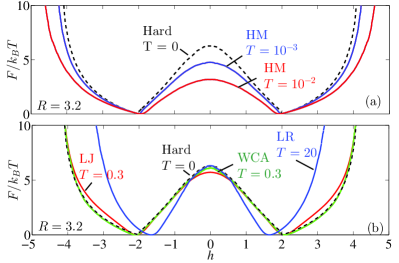
Figure 2: (Color online) (a) The free energy landscape for the harmonic (“HM”) interaction potential. $R=3.2$ and the temperatures are as indicated. (b) Free energy landscapes for interactions as indicated, where “LR” designates the long-range potential, “LJ” the Lennard-Jones potential, and “WCA” the Weeks-Chandler-Andersen potential. $R=3.2$ and the temperatures are as indicated, chosen so that the barrier height at $h=0$ is comparable for the different interaction potentials.

The other features of the free energy landscape shown in Fig. 2(a) are straightforward to understand. There are two symmetrically located minima close to $h=\pm 2$ that correspond to the most probable states for the three particles hunter12pre . For large values of $|h|$, the particles are forced to interact with the confining wall. This causes the free energy to grow dramatically due to the large potential energy penalty.

Figure 2(b) shows free energy landscapes for other interaction potentials, with temperatures chosen so that the barrier height is approximately the same for each, and $R=3.2$ kept constant. The shapes are all qualitatively similar, although the long range potential has particles confined to a smaller range of $h$. For the hard particle case, the minima occur precisely at $h=\pm 2$ hunter12pre . For the other potentials, the locations of the minima vary with $T$. For the LR and LJ potentials, one can compute the configuration that minimizes $U$, and the $h$ that minimize $F(h)$ are fairly close to the $h$ for those minimal $U$ configurations. The $T$ dependence, however, makes it clear that minimizing the free energy is not the same as minimizing the potential energy. Maximizing entropy plays a role as well in determining the $h$ that minimizes $F(h)$. As previously reported, in the hard model, $\partial F/\partial h$ is discontinuous at $h=\pm 2$ hunter12pre . However, this derivative is continuous everywhere in all of the soft models.

III.2 Dynamics and free energy barriers

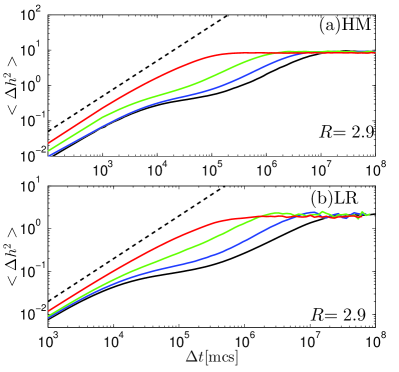
Figure 3: (Color online) (a) Mean-square displacement in $h$ space for the harmonic (“HM”) interaction potential. $R=2.9$ and $T=10^{-1},10^{-2},10^{-2.2},10^{-2.4}$ (from top to bottom, red to black). The dashed line has a slope of 1. (b) Mean-square displacement in $h$ space for the long-range (“LR”) interaction potential. $R=2.9$ and $T=10^{6},10^{4.6},10^{4.2},10^{4}$ (from top to bottom, red to black). The dashed line has a slope of 1.

The dynamics are straightforward when considering $h(t)$. Often, $h(t)$ stays close to the values $h_{\rm min}$ that minimize the free energy landscape (Fig. 2), but occasionally $h(t)$ switches sign. We quantify the dynamics by plotting the mean square displacement (MSD) $\langle\Delta h^{2}\rangle$ as a function of lag time $\Delta t$ in Fig. 3 for the harmonic potential (a) and long-range potential (b). At the shortest times, particles diffuse fairly freely. At intermediate time scales, the MSD starts to level off, reflecting that the system is trapped in one of the probable states shown in Fig. 1(a,c). At longer time scales, the system can swap between these two states, and the MSD begins to rise again. At the longest time scales shown in Fig. 3, the MSD levels off due to the finite system size.

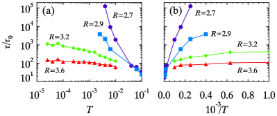
Figure 4: (Color online) Dependence of $\tau$ on $T$ and $R$ in harmonic potential system. Curves in different colors show the life time as a function of $T$ with different $R$ as indicated. The lifetimes $\tau$ are normalized by $\tau_{0}=1/2D$, the time a free particle would take on average to diffuse a distance of 1, using the diffusion constant $D$ from the simulation.

To quantify the transition time scale $\tau$, we measure the average time between sign changes of $h$. However, during a transition, there are often small fluctuations right around $h=0$ that are not true transitions. To avoid biasing $\tau$ toward lower time scales, we stipulate that once $h=0$ is crossed, the system must move a further distance $\Delta{h}=1$ before returning hunter12pre ; our results are not sensitive to this choice. The probability distribution of time scales $P(\tau)$ is exponentially distributed so the mean value gives the appropriate time scale, which we plot in Fig. 4 as a function of temperature (a) and inverse temperature (b). The two largest system sizes $R$ show a horizontal leveling off of $\tau$ at cold temperatures. This is the limit where the soft particles behave as hard particles, and $\tau$ reaches the value seen for purely hard particles hunter12pre . For the smaller system sizes, particles must overlap to have a transition, and so as $T\rightarrow 0$ this becomes rare and $\tau$ diverges. Were any of these systems to be Arrhenius with a temperature-independent potential energy barrier, the data in Fig. 4(b) would fall on a straight line; that they do not indicates that the system is non-Arrhenius.

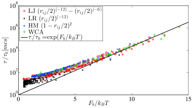
Figure 5: The lifetime grows exponentially with the free energy barrier $F_{b}$ as $F_{b}\rightarrow\infty$, as indicated by the solid line. The symbols are as indicated, and correspond to a variety of $R$ and $T$ values; for specific ranges of $R$ and $T$, see ranges shown in Figs. 4, 6, and 9.

An alternate way to think of Arrhenius behavior is in terms of the free energy barrier for transitions, $F_{b}$. Calculating the free energy landscapes as in Fig. 2 allows us to determine $F_{b}=F(h=0)$. Transitions are less frequent with higher $F_{b}$. Figure 5 verifies that $\tau$ grows Arrheniusly as a function of $F_{b}$, $\tau\sim\exp(\beta F_{b})$ as $F_{b}\rightarrow\infty$. The deviations seen for small $F_{b}$ are due to large system sizes: for larger systems, it simply takes longer for particles to move to the transition state hunter12pre . The details of this vary depending on the potential. Additionally, the vertical spread of symbols for a given potential for $F_{b}\lesssim 5$ reflects that different $R$ and $T$ values can have the same $F_{b}$. Nonetheless, the collapse of the data at larger $F_{b}$ indicates that $\tau$ grows Arrheniusly with $F_{b}$ precisely where the dynamics are slowest.

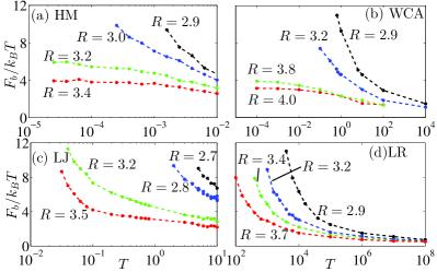
Figure 6: (Color online) Dependence of $\frac{F_{b}}{k_{B}T}$ on $T$ and $R$. Curves in different colors show the free energy barrier as a function of $T$ with different $R$ as indicated. The interaction potentials are (a) harmonic (“HM”), (b) WCA, (c) Lennard-Jones, (d) long-range (“LR”). (As discussed in Sec. II, recall that the specific values of $T$ are not comparable between the different potentials.)

Our primary interest is understanding the cause of glassy dynamics in our system. In other words, we’d like to understand how $\tau$ grows large (equivalently, how $F_{b}$ grows large) as we decrease $T$ and/or decrease $R$. Figure 6 shows $F_{b}/k_{B}T$ as a function of $T$ for different particle types. In each panel, the different curves are for different system sizes $R$. As expected, $F_{b}/k_{B}T$ grows with decreasing $T$ and with decreasing $R$. Panels (a) and (b) show some curves with qualitatively different behavior, in that $F_{b}/k_{B}T$ goes to a plateau as $T\rightarrow 0$. As with Fig. 4, this is because of the behavior of the free energy landscape shown in Fig. 2(a) for these two finite-ranged potentials: for large system sizes $R$, even at $T=0$ the particles can rearrange without overlapping. For large $R$, the plateau values for $F_{b}$ seen in Fig. 6(a,b) are precisely the free energy barrier heights for hard disks hunter12pre . For this argument to work, the system size $R$ must exceed a critical value, $R_{c}=3$ for the harmonic potential and $R_{c}=3.245$ for the WCA potential (as discussed at the end of Sec. II). For $R<R_{c}$, particles must overlap at $h=0$ with $U>0$, and so as $T\rightarrow 0$ the free energy barrier $F_{b}$ will diverge. For the LJ and LR potentials, at $h=0$ we always have $U>0$ and so not surprisingly $F_{b}$ diverges in all cases at low temperatures, with the details depending on $R$.

These behaviors raise an interesting question. In the cases of Fig. 6(a,b) with a plateau, the system approaches the hard disk behavior as $T\rightarrow 0$. For hard disks, this free energy barrier is entirely an entropic barrier hunter12pre . However, clearly for many other cases in Fig. 6, the free energy barrier is at least in part due to the potential energy component of the barrier. To what extent in any of these cases can the free energy barrier be ascribed to entropy, and to what extent to potential energy?

III.3 Simple models for the transition state

To understand the interplay of entropy and potential energy at the transition state ($h=0$) for our three particle system, we consider a simple model for the transition state. Consider a system moving along a reaction coordinate $h$ with a flat energy landscape, except for a barrier at $h=0$. At $h=0$, we will assume there is a second coordinate $x$ in the orthogonal direction. In the three particle system, this would account for other degrees of freedom for the particle locations subject to the constraint $h=0$. We examine three ideas for $U(x)$, sketched in Fig. 7.

First consider Model 1 [Fig. 7(a)], where we let $x$ be constrained on the interval $0\leq x\leq 1$ and the potential energy barrier depends on $x$ as:

$$U(x)=0,\ \ 0\leq x<\delta$$ (7)

$$U(x)=U_{0},\ \ \delta\leq x\leq 1$$ (8)

so that the system can either make a transition at zero potential energy cost, or with a finite cost $U_{0}>0$.

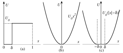
Figure 7: Sketch of three simple potential energy landscapes. (a) Model 1. (b) Model 2. (c) Model 3.

Attempts to cross with zero potential energy cost occur with probability

$$p_{1}=\delta$$ (9)

and these attempts always succeed. Attempts to cross elsewhere occur with probability $(1-\delta)$ and succeed with probability $\exp(-U_{0}/k_{B}T)$; thus the likelihood of a barrier crossing taking this pathway is

$$p_{2}=(1-\delta)\exp(-U_{0}/k_{B}T).$$ (10)

The crossing attempt entirely fails with probability $1-p_{1}-p_{2}$. If attempts are made with a time scale $\tau_{0}$, then the mean transition time can be shown to be

$$\tau=\frac{\tau_{0}}{p_{1}+p_{2}}.$$ (11)

The question to consider, then, is what this transition looks like in terms of a free energy barrier, if we average over the coordinate $x$? Two limits are immediately obvious. If $U_{0}/k_{B}T$ is sufficiently large, $p_{1}\gg p_{2}$ and the transition rate is governed by an entropic barrier. In the converse limit, if $\delta$ is sufficiently small, the $U=0$ pathway is vanishingly rare ($p_{1}\ll p_{2}$) and transitions are governed by the potential energy barrier $U_{0}$. In between these limits, one can think of this system as having an effective free energy barrier that is due to both potential energy and entropy. The mean potential energy the system has when the barrier is crossed is given by

$$\beta\langle U\rangle=\frac{\beta U_{0}p_{2}}{p_{1}+p_{2}}$$ (12)

using $\beta=1/k_{B}T$. The partition function at the crossing is given by $Z=p_{1}+p_{2}$, the free energy barrier height is $\beta F=-\ln Z=-\ln(p_{1}+p_{2})$, and the entropy can be derived as

$$\beta TS=-\beta T\frac{\partial F}{\partial T}=\ln(p_{1}+p_{2})+\beta\langle U\rangle$$ (13)

(which is also apparent from $F=U-TS$).

The conclusion is that while the potential energy surface is $T$-independent and always has a $U=0$ transition pathway, the free energy barrier depends on $T$ and on average requires nonzero potential energy for the transition. Given that $p_{2}$ depends on $T$, Eqns. 12 and 13 show that both the potential energy and entropy contributions to the free energy barrier depend on $T$.

We next consider the more realistic Model 2, where the transition has a harmonic potential with respect to the coordinate $x$:

$$U(x)=U_{0}x^{2}.$$ (14)

For this potential, the mean potential energy required is $\beta\langle U\rangle=1/2$ (equipartition). In the interesting limit $T\rightarrow 0$, the free energy barrier grows as $\beta F\sim|\ln T|$. As the potential energy contribution is independent of $T$, the barrier growth is due to entropy: at low temperatures the system only crosses at $|x|\lesssim\sqrt{k_{B}T/U_{0}}$. As with Model 1, while $U(x)$ is independent of $T$, the free energy barrier depends on $T$.

Finally, we consider model 3 which is a hybrid of the previous two models:

$$U(x)=0,\ \ |x|<\delta$$ (15)

$$U(x)=U_{0}(|x|-\delta)^{2},\ \ |x|\geq\delta.$$ (16)

In this model, the mean potential energy required to cross the barrier is $\beta\langle U\rangle=\frac{1}{2}({1+2\delta\sqrt[]{\frac{\beta U_{0}}{\pi}}})^{-1}$. At low temperature and with large $\delta$, the system prefers to cross within the region $|x|<\delta$ where potential energy is zero. In this case, $\delta\sqrt[]{\frac{\beta U_{0}}{\pi}}\rightarrow\infty$, and $\beta\langle U\rangle\rightarrow 0$. For small $\delta$ and/or large $T$, the average potential energy found when crossing the barrier is larger. At high temperature and with small $\delta$, when $\delta\sqrt[]{\frac{\beta U_{0}}{\pi}}\rightarrow 0$ $,\beta\langle U\rangle\rightarrow 1/2$, which is same as model 2.

To be clear, for these models we are really interested in the case where the system climbs a potential energy hill to reach the transition state $h=0$. We are then considering how the system crosses through the $h=0$ state, and concluding that this requires additional potential energy (on average) and also navigating an entropic barrier. In other words, merely having enough potential energy to reach the saddle is insufficient, as threading through the saddle’s lowest point is of low probability. In all of these simple models of the transition state, the transition time scale will be

$$\tau=\tau_{0}\exp(\beta U_{\rm min})\exp(\beta F)$$ (17)

where $U_{\rm min}$ is the potential energy of the saddle’s lowest point, and $F$ is the additional free energy barrier associated with the $h=0$ potential energy landscape cross-section. The $\exp(\beta U_{\rm min})$ contribution gives Arrhenius scaling with $T$, and the $\exp(\beta F)$ contribution provides additional non-Arrhenius scaling as $F$ grows with decreasing $T$, as shown above. In many situations, the $\exp(\beta U_{\rm min})$ term dominates, but it depends on the details as will be shown below.

III.4 Barriers: Energy and Entropy

This discussion motivates us to divide the free energy barrier in our three-particle simulations into energetic and entropic components. As $F=U-TS$, we consider the free energy barrier to be:

$$\beta F_{b}=\beta U_{b}+S_{b}$$ (18)

where as usual, $k_{B}=1$. The relevant quantities are illustrated in Fig. 8. $h_{\rm min}$ is the value of $h$ that minimizes the free energy. The contribution of potential energy to the barrier is defined as $U_{b}=\langle U\rangle(0)-\langle U\rangle(h_{\rm min})$. $\langle U\rangle$ is the black curve indicated by $U_{b}$ in Fig. 8, and is averaged over $\geq 20$ barrier crossings. Equation 18 lets us calculate $S_{b}$ from $F_{b}$ and $U_{b}$. Note that the definition of $S_{b}$ differs from $U_{b}$ by a minus sign: $S_{b}=S(h_{\rm min})-S(h)>0$, such that it is positive (and thus a barrier). The minimum possible potential energy for each value of $h$ is the thin red curve in Fig. 8 which is at zero for most values of $h$. We define $U_{\rm min}$ as the minimum potential energy needed to cross $h=0$ if the system finds the optimum transition path, as indicated in Fig. 8. It is clear from Fig. 8 that $U_{b}$ will almost always be larger than $U_{\rm min}$, although a rare exception for the Lennard-Jones potential will be described below. $U_{\rm min}$ is a quantity we can derive analytically for each interaction potential, while $U_{b}$ is determined from the simulation data. $U_{\rm min}$ is temperature independent, in contrast to $U_{b}$, $S_{b}$, and $F_{b}$. We wish to see what conditions allow $S_{b}$ or $U_{b}$ to dominate the free energy barrier, and also to gain some intuition about non-Arrhenius temperature dependence in general. Note that simulation times become nearly intractable when $\beta F_{b}=\beta U_{b}+S_{b}\gtrsim 10$, thus limiting how much of the growth of the barriers we can study.

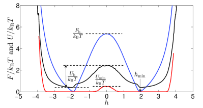
Figure 8: (Color online) The free energy landscape for the harmonic (“HM”) interaction potential. $R=2.9$ and $T=10^{-2.2}$.The blue curve is the free energy landscape. The black curve is the potential energy landscape based on $\langle U\rangle$ in $h$ space. The red curve is the minimum potential energy, $U_{\rm min}$, in $h$ space. $F_{b}/k_{B}T$, $U_{b}/k_{B}T$, and $U_{\rm min}/k_{B}T$ are as indicated. $h_{\rm min}$ is the value that minimizes $F$.

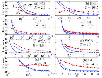
Figure 9: (Color online) Data for the potential energy barrier and entropy barrier for a variety of interaction potentials, temperatures, and system sizes $R$, as indicated. The solid curves indicate $U_{\rm min}$, the theoretical minimum potential energy barrier. The symbols indicate measured values (from the simulation data), connected by straight dashed lines. The meanings of the curves are all as labeled in (a). The interaction potentials are (a,b) harmonic (‘HM’), (c,d) long-range (‘LR’),(e,f) Weeks-Chandler-Andersen (‘WCA’) and (g,h) Lennard-Jones (‘LJ’).

Figure 9(a) shows data for the harmonic interaction potential for $R=2.6$. As $R<3$, the particles must overlap at $h=0$ and thus $U_{\rm min}>0$. The graph shows that as $T\rightarrow 0$, both $\beta U_{b}$ and $S_{b}$ grow. The growth of $\beta U_{b}$ is more significant, pushed up by $\beta U_{\rm min}$. This situation is analogous to Model 2 from Sec. III.3, where $U_{b}\approx U_{\rm min}+\frac{1}{2}k_{B}T$ and $S_{b}\approx|\ln T|$. Given the slow growth of $S_{b}$, the free energy barrier is dominated by $U_{\rm min}$.

Figure 9(b) shows complementary data for the harmonic interaction potential as a function of $R$ at fixed $T=10^{-2}$. Given the finite range for the potential, $U_{\rm min}=0$ for $R\geq 3$, although $U_{b}>0$ as the particles overlap for some crossings. The $R>3$ case is analogous to Model 3, whereas $R<3$ is analogous to Model 2. The data in Fig. 9(b) show that entropy plays a smaller role for small $R$, where the free energy barrier is dominated by the potential energy. For this interaction potential, $U_{\rm min}\sim(R-3)^{2}$ for $R<3$; the data show that $S_{b}$ is nearly constant as a function of $R$.

Figure 9(c,d) shows the comparisons of entropic barrier and potential barrier for the LR potential. For large $T$ or large $R$ cases, $S_{b}>\beta U_{b}$. In the converse cases, the opposite is true. As the system becomes slower with a large free energy barrier, the free energy barrier is strongly determined by the potential energy component.

For the WCA data shown in Fig. 9(e,f), $U_{\rm min}$ goes to zero at $R=3.245$, although as before we still have $\beta U_{b}>0$. For the WCA potential, we see a more dramatic growth of $U_{b}$ with decreasing $T$ [panel (e)] and with decreasing $R$ [panel (f)]. It appears that if we further shrink the system size in panel (f), $U_{b}$ will eventually grow larger than $S_{b}$. The growth of $S_{b}$ at small $R$ is not as strong as the growth of $\beta U_{\rm min}$, and since $U_{b}>U_{\rm min}$, this further suggests that $\beta U_{b}$ will be larger than $S_{b}$ for smaller systems.

Figure 9(g,h) shows the comparisons of entropic barrier and potential barrier for the LJ potential. For high $T$ cases [panel (g)], $S_{b}>\beta U_{b}$, with the opposite occurring as $T\rightarrow 0$. Panel (h) shows that at a fixed $T$, with decreasing $R$ both $S_{b}$ and $\beta U_{b}$ grow, with the latter growing more dramatically. It appears that if we further shrink the system size in panel (h), $U_{b}$ will eventually grow larger than $S_{b}$.

Unusual behavior is seen for the LJ potential in Fig. 9(g,h), where $U_{b}<U_{\rm min}$ with large $R$ and low $T$. This can be understood given the differences between our definitions of $U_{b}$ and $U_{\rm min}$. $U_{min}$ considers the difference in potential energy between the lowest potential energy path at the saddle point ($h=0$) and the lowest potential energy the particles can obtain given $R$. The latter corresponds to a configuration where the centers of the particles form an equilateral triangle with side length $=2.24$, corresponding to $h=1.94$. However, this configuration is itself an unlikely configuration, and for example when $h=1.94$ the three particles will often be in a configuration with slightly higher potential energy than the absolute minimum. This is essentially the same argument put forth in Sec. III.3, that the average potential energy experienced by the system is not the minimum value. Thus, the measured potential energy difference $U_{b}$ will often be between a slightly higher value for both $h=0$ and $h=h_{\rm min}$, such that their difference $U_{b}=U(0)-U(h_{\rm min})<U_{\rm min}$. This is not the case for the other interaction potentials, probably because the potential energy is a flatter function of $h$ around $h_{\rm min}$ for the other interaction potentials.

Some general conclusions can be drawn from all of the data of Fig. 9. First, in most of the cases, $U_{b}>U_{\rm min}$, confirming the intuition from Sec. III.3: that crossing the saddle point in the potential energy landscape is not typically done at the minimal potential energy path through that saddle point. Second, Fig. 9(a,c,e) demonstrates that $\beta U_{b}$ and $S_{b}$ both depend on $T$ and are larger for colder temperatures: and thus these barriers behave non-Arrheniusly. In particular, these barriers are not simply based on $\beta U_{\rm min}$.

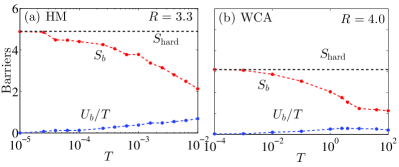
Figure 10: (Color online) The potential barrier and entropy barrier for (a) the harmonic interaction potential and (b) the WCA interaction potential. The system sizes $R$ are as indicated, and chosen such that the minimum potential energy barrier is $U_{\rm min}=0$. The horizontal dashed lines indicate the free energy barrier for the hard disk case.

The finite-ranged potentials (harmonic and WCA) allow us to look at cases where $U_{\rm min}=0$. As noted in the discussion of Fig. 6(a,b), when $U_{\rm min}=0$ the free energy barriers reach a plateau as $T\rightarrow 0$ corresponding to the hard disk limit (the horizontal dashed lines). The data for the energy and entropy barriers are shown for two of these cases in Fig. 10. These data match the qualitative behavior predicted by Model 3 (Sec. III.3). At low $T$, $\beta U_{b}\approx 0$ and $S_{b}$ approaches the hard disk result. At high $T$, $\beta U_{b}\approx\frac{1}{2}$ and the entropic contribution decreases as more microstates are possible at $h=0$. For different temperatures, the trade-off between crossing with zero or finite potential energy changes, due to the entropic penalty of choosing the zero potential energy pathway, which is weighted by the temperature.

IV Conclusions

We studied a free energy landscape of a simple model possessing some qualitative features of a glass transition. The model’s slow dynamics are governed by a free energy barrier which we directly measure in simulations. The barrier height is determined both by entropy and potential energy. The relative contributions of each of these depend on temperature $T$. In particular, for fixed system size $R$, the potential energy landscape is independent of $T$, yet the effective potential energy barrier height, entropic barrier height, and overall free energy barrier all depend on $T$. This leads to non-Arrhenius temperature dependence. We conjecture that for cases with more particles, entropy plays an even more important role in cooperative rearrangements, as suggested in 1965 by Adam and Gibbs adam65 and discussed by many authors subsequently. In fact, our model is quite in the spirit of Adam and Gibbs, in that rearrangements require coordinated motion of all three particles [Fig. 1(b)] which results in an entropic penalty.

There are qualitative differences between our model results and non-Arrhenius behavior seen in glass-forming systems. First, the onset of slow dynamics in our model requires temperature changes of several orders of magnitude (Fig. 6), whereas similar changes in glassy materials require a temperature decrease of only 10-20% biroli13 ; ediger12 ; cavagna09 ; dyre06 ; angell95 . Second, in our model, as $T\rightarrow 0$, the potential energy component of the barrier may become more important than entropy, suggesting a possible recovery of Arrhenius behavior at the lowest $T$ (Fig. 9). However, this is not completely clear from our data as the $T\rightarrow 0$ behavior requires prohibitively long simulation runs. Both of these differences between our simple model and glassy behavior might disappear for larger numbers of particles, but then we would lose the ability to fully visualize the free energy landscape (Fig. 2). It is certainly known that near the glass transition, rearrangements can involve far more than three particles perera99 ; doliwa00 , which would likely enhance the sensitivity to temperature. While we do not provide a realistic description of the $N\rightarrow\infty$ limit of a glass transition, we have demonstrated connections between the free energy landscape, free energy barriers, and non-Arrhenius temperature dependence in our model glassy system.

We thank M. E. Cates, F. Family and G. L. Hunter for helpful discussions. This work has been supported financially by the NSF (CMMI-1250199/-1250235).

References

- (1) G. Biroli and J. P. Garrahan. Perspective: The glass transition. J. Chem. Phys., 138, 12A301 (2013).
- (2) M. D. Ediger and P. Harrowell. Perspective: Supercooled liquids and glasses. J. Chem. Phys., 137, 080901 (2012).
- (3) A. Cavagna. Supercooled liquids for pedestrians. Phys. Rep., 476, 51 (2009).
- (4) J. C. Dyre. Colloquium : The glass transition and elastic models of glass-forming liquids. Rev. Mod. Phys., 78, 953 (2006).
- (5) C. A. Angell, K. L. Ngai, G. B. McKenna, P. F. McMillan, and S. W. Martin. Relaxation in glassforming liquids and amorphous solids. J. App. Phys., 88, 3113 (2000).
- (6) L. Cipelletti and L. Ramos. Slow dynamics in glasses, gels and foams. Curr. Op. Coll. Int. Sci., 7, 228 (2002).
- (7) M. Goldstein. Viscous liquids and the glass transition: A potential energy barrier picture. J. Chem. Phys., 51, 3728 (1969).
- (8) P. G. Debenedetti and F. H. Stillinger. Supercooled liquids and the glass transition. Nature, 410, 259 (2001).
- (9) F. H. Stillinger. A topographic view of supercooled liquids and glass formation. Science, 267, 1935 (1995).
- (10) F. Sciortino. Potential energy landscape description of supercooled liquids and glasses. J. Stat. Mech., 2005, P05015 (2005).
- (11) A. Heuer. Exploring the potential energy landscape of glass-forming systems: from inherent structures via metabasins to macroscopic transport. J. Phys.: Cond. Matter, 20, 373101 (2008).
- (12) F. H. Stillinger and T. A. Weber. Hidden structure in liquids. Physical Review A, 25, 978 (1982).
- (13) S. Sastry, P. G. Debenedetti, and F. H. Stillinger. Signatures of distinct dynamical regimes in the energy landscape of a glass-forming liquid. Nature, 393, 554 (1998).
- (14) T. Pérez-Castañeda, R. J. Jiménez-Riobóo, and M. A. Ramos. Two-level systems and boson peak remain stable in 110-million-year-old amber glass. Phys. Rev. Lett., 112, 165901 (2014).
- (15) P. Charbonneau, J. Kurchan, G. Parisi, P. Urbani, and F. Zamponi. Fractal free energy landscapes in structural glasses. Nature Comm., 5, 3725 (2014).
- (16) F. H. Stillinger and T. A. Weber. Packing structures and transitions in liquids and solids. Science, 225, 983 (1984).
- (17) M. H. Cohen and D. Turnbull. Molecular transport in liquids and glasses. J. Chem. Phys., 31, 1164 (1959).
- (18) L. V. Woodcock and C. A. Angell. Diffusivity of the hard-sphere model in the region of fluid metastability. Phys. Rev. Lett., 47, 1129 (1981).
- (19) R. J. Speedy. The hard sphere glass transition. Mol. Phys., 95, 169 (1998).
- (20) R. K. Bowles and R. J. Speedy. Five discs in a box. Physica A, 262, 76 (1999).
- (21) S. S. Ashwin and R. K. Bowles. Complete jamming landscape of confined hard discs. Phys. Rev. Lett., 102, 235701 (2009).
- (22) G. L. Hunter and E. R. Weeks. Free-energy landscape for cage breaking of three hard disks. Phys. Rev. E, 85, 031504 (2012).
- (23) D. N. Perera and P. Harrowell. Relaxation dynamics and their spatial distribution in a two-dimensional glass-forming mixture. J. Chem. Phys., 111, 5441 (1999).
- (24) B. Doliwa and A. Heuer. Cooperativity and spatial correlations near the glass transition: Computer simulation results for hard spheres and disks. Phys. Rev. E, 61, 6898 (2000).
- (25) L. Berthier and T. A. Witten. Glass transition of dense fluids of hard and compressible spheres. Phys. Rev. E, 80, 021502 (2009).
- (26) N. Xu, T. K. Haxton, A. J. Liu, and S. R. Nagel. Equivalence of glass transition and colloidal glass transition in the hard-sphere limit. Phys. Rev. Lett., 103, 245701 (2009).
- (27) M. Schmiedeberg, T. K. Haxton, S. R. Nagel, and A. J. Liu. Mapping the glassy dynamics of soft spheres onto hard-sphere behavior. Europhys. Lett., 96, 36010 (2011).
- (28) C. A. Angell. Formation of glasses from liquids and biopolymers. Science, 267, 1924 (1995).
- (29) C. S. O’Hern, L. E. Silbert, A. J. Liu, and S. R. Nagel. Jamming at zero temperature and zero applied stress: The epitome of disorder. Phys. Rev. E, 68, 011306 (2003).
- (30) D. J. Durian. Foam mechanics at the bubble scale. Phys. Rev. Lett., 75, 4780 (1995).
- (31) J. E. Lennard-Jones. Cohesion. Proc. Phys. Soc., 43, 461 (2002).
- (32) H. C. Andersen, J. D. Weeks, and D. Chandler. Relationship between the hard-sphere fluid and fluids with realistic repulsive forces. Phys. Rev. A, 4, 1597 (1971).
- (33) N. Metropolis, A. W. Rosenbluth, M. N. Rosenbluth, A. H. Teller, and E. Teller. Equation of state calculations by fast computing machines. J. Chem. Phys., 21, 1087 (1953).
- (34) G. Adam and J. H. Gibbs. On the temperature dependence of cooperative relaxation properties in glass-forming liquids. J. Chem. Phys., 43, 139 (1965).