Small–scale anisotropies of cosmic rays from relative diffusion

Abstract:

The arrival directions of multi–TeV cosmic rays show significant anisotropies at small angular scales. It has been argued that this small scale structure is reflecting the local, turbulent magnetic field in the presence of a global dipole anisotropy in cosmic rays as determined by diffusion. This effect is analogous to weak gravitational lensing of temperature fluctuations of the cosmic microwave background. We show that the non–trivial power spectrum in this setup can be related to the properties of relative diffusion and we study the convergence of the angular power spectrum to a steady–state as a function of backtracking time. We also determine the steady–state solution in an analytical approach based on a modified BGK ansatz. A rigorous mathematical treatment of the generation of small scale anisotropies will help in unraveling the structure of the local magnetic field through cosmic ray anisotropies.

1 Introduction

The arrival directions of cosmic rays (CRs) are highly isotropic, to about one part in $10^{4}$ at TeV–PeV energies. Given the discrete nature of their sources, this requires an efficient mechanism for isotropising their directions. Resonant interactions of CRs with turbulent magnetic fields, that lead to pitch–angle scattering and induce spatial diffusion, can provide this randomisation.

In a diffusive approximation to CR transport, the (microscopic) power spectrum of the turbulent magnetic field is related to the (macroscopic) transport parameters, like the pitch–angle or diffusion coefficients. The phase space density, averaged over a statistical ensemble of turbulent magnetic fields, is expanded into an isotropic part $f_{0}$ and anisotropic corrections $f_{i}(\mu)$ [1]. (Here, $\mu$ is the pitch angle cosine.) Anticipating that the anisotropic corrections are much smaller than the isotropic part, the dipole anisotropy, defined by the first moment in pitch angle cosine, can be related to the spatial gradient of the isotropic part, $n=4\pi f_{0}$. The dipole term in the angular power spectrum of the relative intensity $\delta I\equiv(4\pi f-n)/n$ then relates to the gradient and the diffusion tensor ${\bf K}$ as,

$$\frac{1}{4\pi}{C_{1}}=\left|\frac{{\bf K}\nabla n}{n}\right|^{2}\,.$$ (1)

Another process contributing is the Compton–Getting effect [2]. Adopting a certain distribution of sources and a (semi–phenomenological), scalar diffusion tensor, it has been shown that the predicted dipole anisotropy is up to two orders of magnitude larger than the observed one [3]. It has been suggested that intermittency effects in the source distribution [4, 5, 6] or (spatially dependent) anisotropic diffusion [7, 8] can mitigate this discrepancy. An attractive solution is the combination of anisotropic diffusion with intermittency effects in the turbulent magnetic fields [9].

Even more surprising, structure in the distribution of arrival directions has been detected at much smaller angular scales, first by MILAGRO [10]. IceCube [11] and HAWC [12] have recently presented measurements of the angular power spectrum of the arrival directions, finding significant power down to angular scales of $\sim 5^{\circ}$ and $\sim 10^{\circ}$, respectively, see Fig. 1. The appearance of structure on scales smaller than the dipole can also be understood in terms of intermittency in the turbulent magnetic fields [13, 14]: Unlike the ensemble–averaged phase space density, the actual phase space density exhibits power on all scales. The particular realisation of the local turbulent magnetic field is thus imprinted on the arrival directions of cosmic rays. In Fig. 1, we show the prediction of the ensemble–averaged angular power spectrum from a fully analytical computation of this effect [14].

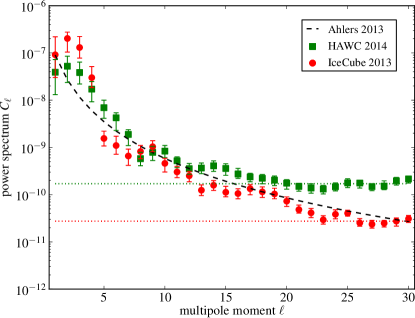
Figure 1: Power spectrum of the CR arrival directions observed by IceCube [11] and HAWC [12]. The horizontal dotted lines indicate the level of statistical noise at the level of $\mathcal{N}\simeq{f_{\rm sky}4\pi}/{N_{\rm CR}}$, where $f_{\rm sky}$ is the effective fraction of the sky that contains $N_{\rm CR}$ collected events. For IceCube we can estimate $f_{\rm sky}\simeq 0.3$ and $\mathcal{N}_{\rm IC}\simeq 2.5\times 10^{-11}$ and for HAWC with $f_{\rm sky}\simeq 0.7$ we have $\mathcal{N}_{\rm HAWC}\simeq 1.8\times 10^{-10}$. The dashed line shows the result of Ref. [14].

In the following, we will support this idea with a combination of analytical and numerical arguments. Specifically, in Sec. 2 we will clarify the relation between the small–scale anisotropies and relative diffusion of CRs. By numerically back–tracking CRs through turbulent magnetic fields, we will show in Sec. 3 how the angular power spectrum develops in time and that convergence to a steady–state is reached for long enough backtracking times. In Sec. 4, we will describe the temporal evolution of the angular power spectrum, starting from Liouville’s theorem and adopting a BGK–like [15] ansatz. We will summarise and conclude in Sec. 5.

2 Relative diffusion

In the following, we study the small, stochastic deviations of the local phase space density $f$ from its ensemble average $\langle f\rangle$, $\delta f\equiv f-\langle f\rangle$. Given a quasi–stationary phase space density at time $t=-T$, $4\pi\langle f\rangle\simeq n-3\hat{\bf p}{\bf K}\nabla n$, the phase space density $f$ at time $t=0$ follows from Liouville’s theorem,

$$4\pi f\simeq 4\pi\delta{f}(-T)+n+({\bf r}(-T)-3\hat{\bf p}(-T){\bf K})\nabla n\,,$$ (2)

where ${\bf r}(-T)$ and ${\bf p}(-T)$ are the position and momentum of a CR particle at time $t=-T$. We can then compute the angular power spectrum at time $t=0$ which is defined as

$$C_{\ell}=\frac{1}{4\pi}\int{\rm d}\hat{\bf p}_{1}\int{\rm d}\hat{\bf p}_{2}\,P_{\ell}(\hat{\bf p}_{1}\hat{\bf p}_{2})f_{1}f_{2}\,,$$ (3)

where $\hat{\bf p}_{i}$ denote unit vectors and $P_{\ell}$ the usual Legendre polynomials. Here and in the following we use the abbreviation $f_{i}=f(t,{\bf r}_{i},{\bf p}_{i})$. We note that due to pitch–angle scattering, the term ${\bf r}(-T)\nabla n$ in eq. 2 will dominate over $-3\hat{\bf p}(-T){\bf K}\nabla n$ at late times. Furthermore, we assume that in the ensemble average and again at late times, fluctuations are uncorrelated, $\langle\delta f_{1}(-T)\delta f_{2}(-T)\rangle=0$. We thus find for the ensemble–averaged angular power spectrum of the relative intensity $\delta I\equiv(4\pi f-n)/n$,

$$\frac{1}{4\pi}{\langle C_{\ell}\rangle}\simeq\int\frac{{\rm d}\hat{\bf p}_{1}}{4\pi}\int\frac{{\rm d}\hat{\bf p}_{2}}{4\pi}P_{\ell}(\hat{\bf p}_{1}\hat{\bf p}_{2})\lim_{T\to\infty}\langle{r}_{1i}(-T){r}_{2j}(-T)\rangle\frac{\partial_{i}n\partial_{j}n}{n^{2}}\,.$$ (4)

This expression can be related to the symmetric part of the relative diffusion coefficient

$$\widetilde{K}^{\rm s}_{ij}=\int\frac{{\rm d}\hat{\bf p}_{1}}{4\pi}\int\frac{{\rm d}\hat{\bf p}_{2}}{4\pi}\lim_{T\to\infty}\frac{1}{4T}\big{\langle}\big{\{}r_{1i}(-T)-r_{2i}(-T)\big{\}}\big{\{}r_{1j}(-T)-r_{2j}(-T)\big{\}}\big{\rangle}\,,$$ (5)

by noting that the sum over all multipoles $\ell\geq 0$ (i.e. the variance of the flux) reads

$$\frac{1}{4\pi}\sum_{\ell\geq 0}(2\ell+1){\langle C_{\ell}\rangle}(T)\simeq 2T{K}^{\rm s}_{ij}\frac{\partial_{i}n\partial_{j}n}{n^{2}}\,,$$ (6)

where the symmetric part of the diffusion tensor ${K}^{\rm s}_{ij}$ is defined through $\langle{r}_{i}(-T){r}_{j}(-T)\rangle\to 2T{K}^{\rm s}_{ij}$ in the limit of large backtracking times $T$. The monopole on the other hand satisfies,

$$\frac{1}{4\pi}{\langle C_{0}\rangle}(T)\simeq 2T\left({K}^{\rm s}_{ij}-\widetilde{K}^{\rm s}_{ij}\right)\frac{\partial_{i}n\partial_{j}n}{n^{2}}\,,$$ (7)

such that the power in higher multipoles is

$$\frac{1}{4\pi}\sum_{\ell\geq 1}(2\ell+1){\langle C_{\ell}\rangle}(T)\simeq 2T\widetilde{K}^{\rm s}_{ij}\frac{\partial_{i}n\partial_{j}n}{n^{2}}\,.$$ (8)

3 Simulation

We now turn to a numerical simulation that backtracks CRs through a turbulent magnetic field. On top of a regular field ${\bf B}_{0}$, we have set up the turbulent field as the sum of $N$ harmonic modes $\delta{\bf B}({\bf x})=\sum_{n=1}^{N}\delta{\bf B}_{n}\cos({\bf k}_{n}{\bf x}+\beta_{n})$ with $N$ random phases $\beta_{n}$ and wave vectors ${\bf k}_{n}$, following Ref. [16]. We choose the amplitudes to satisfy $\delta{\bf B}_{n}\perp{\bf k}_{n}$ and $|\delta{\bf B}_{n}|^{2}\propto k_{n}^{3}/(1+(k_{n}L_{c})^{\gamma})$ with coherence scale $L_{c}$, giving a Kolmogorow–type phenomenology for $\gamma=11/3$. The level of turbulence is parametrised by $\sigma$ with $\sum|\delta{\bf B}_{n}|^{2}=2\sigma^{2}{\bf B}_{0}^{2}$. We sample the CR directions at time $t=0$, $\hat{\bf p}_{i}(0)$, isotropically on a HEALPix [17] grid with resolution parameter $n_{\rm side}=32$, for a total of $N_{\rm pix}=12288$ trajectories per random field configuration, and we evaluate 120 such configurations. For the simulations, we choose $\sigma^{2}=1$, $\lambda_{\rm min}=0.01\,L_{c}$ and $\lambda_{\rm max}=100\,L_{c}$ with $k=2\pi/\lambda$. Whereas in the Galaxy with $L_{c}\sim 30\,\text{pc}$ and $B_{0}\sim 3\,\mu\text{G}$ the gyroradius of $10\,\text{TeV}$ CRs is much smaller than the coherence length, $r_{L}/L_{c}\sim 10^{-5}$, we here fix $r_{L}=0.1\,L_{c}$ to reach the (temporally) asymptotic regime within reasonable computing times.

In Fig. 2, we show the average angular power spectrum $C_{\ell}$ of the relative intensity $\delta I$ as a function of backtracking time $T$, obtained by multipole expansion with the HEALPix utilities. We show the results for a CR gradient parallel and perpendicular to the regular magnetic field ${\bf B}_{0}$ by the solid and dotted lines, respectively. Black lines denote the ensemble–averaged dipole, magenta lines show the standard dipole of the ensemble–averaged phase space density. As expected, the latter is smaller than the former. For $2\leq\ell\leq 9$, the multipoles are shown by the green lines. As we are dealing with the angular power spectrum of the relative intensity, there is a small residual monopole which is shown by the blue lines.

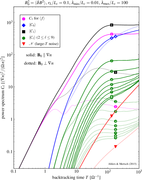
Figure 2: The evolution of the ensemble-averaged power spectrum (4) for a CR gradient parallel (solid lines) and perpendicular (dotted lines) to the regular magnetic field and the 3D turbulence model discussed in the main text. We show results in terms of the dipole $\langle C_{1}\rangle$ (black), monopole $\langle C_{0}\rangle$ (blue) and medium-$\ell$ multipoles (green). We also show the asymptotic noise level (9) (red) and the dipole prediction (1) of standard diffusion (magenta) evaluated by the replacement $\langle{\rm r}_{1}{\rm r}_{1}\rangle\to\langle{\rm r}_{1}\rangle\langle{\rm r}_{2}\rangle$ in Eq. (4).

At late times ($t\Omega\gtrsim 100$ for our parameters, $\Omega$ being the gyrofrequency), the angular power spectrum is exhibiting an asymptotic behaviour. This is reflecting the fact that the arrival directions measured at any one position are only sensitive to the particular realisation of the local turbulent magnetic field. Memory of the anisotropies at even earlier times is lost. Note that the higher multipoles are more strongly effected by shot noise which is due to the finite number of trajectories and shown by the red lines in Fig. 2. Again for large backtracking times, the shot noise can be estimated as

$$\mathcal{N}\simeq\frac{4\pi}{N_{\rm pix}}2TK^{\rm s}_{ij}\frac{\partial_{i}n\partial_{j}n}{n^{2}}\,.$$ (9)

In Fig. 3 we show the best estimator for the true power spectrum $\widehat{C}_{\ell}=\langle C_{\ell}\rangle-\mathcal{N}$ and its noise variance for three different times and for parallel and perpendicular CR gradients, respectively. For the limited number of trajectories considered here, it might be difficult to distinguish between noise variance and cosmic variance which is why we here show the former only. Note the concave shape of the angular power spectrum which is also seen in the experimental data (see Fig. 1) and the convergence to the asymptotic form for late times.

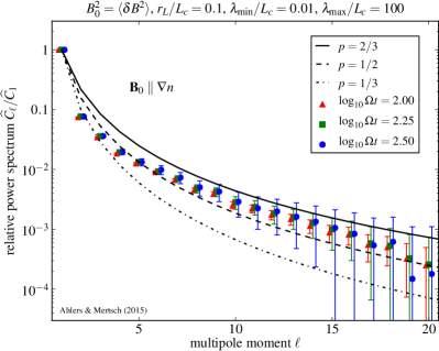
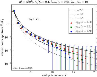
Figure 3: The power spectrum estimator $\widehat{C}_{\ell}=\langle C_{\ell}\rangle-\mathcal{N}$ (normalized to $\widehat{C}_{1}$) for parallel (left plot) and perpendicular (right plot) CR gradient for the data shown in Fig. 2 at three different backtracking times. We also show the noise variance level of the data. The three lines correspond to the prediction of a relative scattering term $\nu_{r}(x)\propto(1-x)^{p}$ in Eq. (16).

4 BGK–like ansatz

In the following, we derive the asymptotic angular power spectrum in a generalisation of the BGK [15] ansatz used in diffusion theory. We start from the Boltzmann equation for the phase space density $f$, again split into an average and a fluctuating part, $f=\langle f\rangle+\delta{f}$. After ensemble averaging, the Boltzmann equation reads [18]

$$\partial_{t}\langle f\rangle+\hat{\bf p}\nabla_{\bf r}\langle f\rangle-i\boldsymbol{\Omega}{\bf L}\langle f\rangle=\left\langle i\boldsymbol{\omega}{\bf L}\delta{f}\right\rangle\,,$$ (10)

where we have introduced the angular momentum operator ${\bf L}=-i{\bf p}\times\nabla_{{\bf p}}$ as well as the rotation vectors ${\boldsymbol{\Omega}}=e{\bf B}_{0}/p_{0}$ and ${\boldsymbol{\omega}}=e\delta{\bf B}/p_{0}$. In eq. (10), the effect of the turbulent magnetic fields is contained in the r.h.s. collision term, $\left\langle i\boldsymbol{\omega}{\bf L}\delta{f}\right\rangle$. In standard diffusion theory, this term is replaced with a friction term following Bhatnagar, Gross & Krook [15] (BGK), that drives the ensemble–averaged phase space distribution to its isotropic mean $n$ with an effective relaxation rate $\nu$, i.e.

$$\left\langle i\boldsymbol{\omega}{\bf L}\delta{f}\right\rangle\simeq-\nu\left(\langle f\rangle-\frac{n}{4\pi}\right)\,.$$ (11)

In order to generalise the BGK ansatz, we note the relation to Brownian motion on the sphere [19] where the diffusion equation reads $\partial_{t}f=-(\nu/2){\bf L}^{2}f$. Therefore, instead of eq. 11, we write

$$\left\langle i\boldsymbol{\omega}{\bf L}\delta{f}\right\rangle\simeq-\frac{\nu}{2}{\bf L}^{2}\langle f\rangle\,.$$ (12)

For the asymptotic angular power spectrum, we solve for the steady–state solution of

$$\partial_{t}\langle f_{1}f_{2}\rangle=\langle f_{1}\left(-\hat{\bf p}_{2}\nabla_{\bf r}+i\boldsymbol{\omega}_{2}{\bf L}+i\boldsymbol{\Omega}{\bf L}\right)f_{2}\rangle+(1\leftrightarrow 2)\,.$$ (13)

and in the spirit of eq. 12 we therefore make the ansatz

$$\langle(i\boldsymbol{\omega}_{1}{\bf L}_{1}+i\boldsymbol{\omega}_{2}{\bf L}_{2})f_{1}f_{2}\rangle\simeq-\left[\nu_{\rm r}(x)\frac{{\bf L}_{1}^{2}+{\bf L}_{2}^{2}}{2}+\nu_{\rm c}(x){\bf J}^{2}\right]\langle f_{1}f_{2}\rangle\,,$$ (14)

with $x=\hat{\bf p}_{1}\hat{\bf p}_{2}$ and ${\bf J}={\bf L}_{1}+{\bf L}_{2}$. This term will lead to mixing and damping of multipoles. Here, we have defined the relative and correlated scattering rates, $\nu_{\rm r}$ and $\nu_{\rm c}$, that depend on the relative distance of the trajectories at early times, or equivalently on the opening angle between trajectories. Note that Eq. (14) is necessarily symmetric under interchange of ${\bf p}_{1}\leftrightarrow{\bf p}_{2}$ as well as ${\bf p}_{i}\leftrightarrow-{\bf p}_{i}$ and is the most general linear approximation of all possible scalar combination of ${\bf L}_{1}$ and ${\bf L}_{2}$. In Eq. (13), we also replace the gradient term in via $\langle f_{1}\hat{\bf p}_{2}\nabla f_{2}\rangle\simeq-3/(4\pi)^{2}\hat{\bf p}_{1}\nabla{n}\hat{\bf p}_{2}{\bf K}\nabla{n}$, assuming that the spatial dependence of $\delta f_{i}$ is small compared to $\langle f_{i}\rangle$ for $f_{i}=\langle f_{i}\rangle+\delta{f}_{i}$.

One can show (see [20] for details), that the asymptotic angular power spectrum satisfies

$$Q_{1}\delta_{\ell 1}=\sum_{k}\langle C_{k}\rangle k(k+1)\frac{2k+1}{2}\int{\rm d}x\,\nu_{\rm r}(x)P_{\ell}(x)P_{k}(x)\,,$$ (15)

where the term $Q_{1}={K}_{ij}{\partial_{i}n\partial_{j}n}/(6\pi)$ is sourcing the dipole. This can be inverted to give

$$\langle C_{\ell}\rangle=\frac{3}{2}\frac{Q_{1}}{\ell(\ell+1)}\int\limits_{-1}^{1}{\rm d}x\frac{x\,P_{\ell}(x)}{\nu_{\rm r}(x)}\,.$$ (16)

We model the unknown dependence of the relative scattering rate on the opening angle $x$ as $\nu_{\rm r}(x)\propto(1-x)^{p}$, with $0<p<1$. This is motivated by the fact that particles along the same trajectory never decorrelate and therefore $\nu_{\rm r}(1)=0$ whereas for $x<1$, $\nu_{\rm r}(x)$ must be positive but finite, and possibly monotonous. In Fig. 3, we show the angular power spectrum for $p=1/3$, $1/2$ and $2/3$. The value $p=1/2$ in particular seems to be reproducing the simulated data rather well.

5 Summary and conclusion

In summary, we have shown how the power in multipole $C_{\ell}$ with $\ell\geq 1$ relates to relative diffusion of CRs. Furthermore, we have investigated the angular power spectrum of the relative intensity of CRs as a function of backtracking time, showing that at late times, the angular power spectrum converges to a steady state. This reflects the fact that the observed anisotropy reflects the local realisation of the turbulent magnetic field and is independent of the anisotropy at much earlier times. Finally, we have also shown that the observed concave form of the angular power spectrum can be reproduced by adopting a BGK–like ansatz for the generalised collision term in the Boltzmann equation. Observations of the small–scale anisotropy therefore encode information about the actual representation of the turbulent magnetic field in our Galactic neighbourhood. Such information could be harvested if the inverse problem of inferring the magnetic field from the distribution of arrival directions were tractable.

References

- [1] J. R. Jokipii, Cosmic-Ray Propagation. I. Charged Particles in a Random Magnetic Field, ApJ 146 (1966) 480.
- [2] A. H. Compton and I. A. Getting, An Apparent Effect of Galactic Rotation on the Intensity of Cosmic Rays, Physical Review 47 (June, 1935) 817–821.
- [3] A. M. Hillas, TOPICAL REVIEW: Can diffusive shock acceleration in supernova remnants account for high-energy galactic cosmic rays?, Journal of Physics G Nuclear Physics 31 (2005) 95.
- [4] V. S. Ptuskin, F. C. Jones, E. S. Seo, and R. Sina, Effect of random nature of cosmic ray sources Supernova remnants on cosmic ray intensity fluctuations, anisotropy, and electron energy spectrum, Advances in Space Research 37 (2006) 1909–1912.
- [5] P. Blasi and E. Amato, Diffusive propagation of cosmic rays from supernova remnants in the Galaxy. II: anisotropy, JCAP 1201 (2012) 011, [arXiv:1105.4529].
- [6] M. Pohl and D. Eichler, Understanding TeV-band cosmic-ray anisotropy, Astrophys.J. 766 (2013) 4, [arXiv:1208.5338].
- [7] C. Evoli, D. Gaggero, D. Grasso, and L. Maccione, A common solution to the cosmic ray anisotropy and gradient problems, Phys. Rev. Lett. 108 (2012) 211102, [arXiv:1203.0570].
- [8] R. Kumar and D. Eichler, Large-scale Anisotropy of TeV-band Cosmic Rays, ApJ 785 (Apr., 2014) 129.
- [9] P. Mertsch and S. Funk, Solution to the cosmic ray anisotropy problem, Phys.Rev.Lett. 114 (2015) 021101, [arXiv:1408.3630].
- [10] A. Abdo, B. Allen, T. Aune, D. Berley, E. Blaufuss, et al., Discovery of Localized Regions of Excess 10-TeV Cosmic Rays, Phys.Rev.Lett. 101 (2008) 221101, [arXiv:0801.3827].
- [11] IceCube Collaboration, M. Aartsen et al., The IceCube Neutrino Observatory Part III: Cosmic Rays, arXiv:1309.7006.
- [12] HAWC Collaboration, A. Abeysekara et al., Observation of Small-scale Anisotropy in the Arrival Direction Distribution of TeV Cosmic Rays with HAWC, arXiv:1408.4805.
- [13] G. Giacinti and G. Sigl, Local Magnetic Turbulence and TeV-PeV Cosmic Ray Anisotropies, Phys.Rev.Lett. 109 (2012) 071101, [arXiv:1111.2536].
- [14] M. Ahlers, Anomalous Anisotropies of Cosmic Rays from Turbulent Magnetic Fields, Phys.Rev.Lett. 112 (2014), no. 2 021101, [arXiv:1310.5712].
- [15] P. Bhatnagar, E. Gross, and M. Krook, A Model for Collision Processes in Gases. 1. Small Amplitude Processes in Charged and Neutral One-Component Systems, Phys.Rev. 94 (1954) 511–525.
- [16] J. Giacalone and J. Jokipii, The Transport of Cosmic Rays across a Turbulent Magnetic Field, Astrophys.J. 520 (1999) 204.
- [17] K. Gorski, E. Hivon, A. Banday, B. Wandelt, F. Hansen, et al., HEALPix - A Framework for high resolution discretization, and fast analysis of data distributed on the sphere, Astrophys.J. 622 (2005) 759–771, [astro-ph/0409513].
- [18] F. C. Jones, The generalized diffusion-convection equation, ApJ 361 (Sept., 1990) 162–172.
- [19] K. Yosida, Brownian Motion on the Surface of the 3-Sphere, Ann. Math. Statist. 20 (1949) 292–296.
- [20] M. Ahlers and P. Mertsch, Small-Scale Anisotropies of Cosmic Rays from Relative Diffusion, arXiv:1506.0548.