Computational Homogenization of Fresh Concrete Flow Around Reinforcing Bars

Abstract

Motivated by casting of fresh concrete in reinforced concrete structures, we introduce a numerical model of a steady-state non-Newtonian fluid flow through a porous domain. Our approach combines homogenization techniques to represent the reinforced domain by the Darcy law with an interfacial coupling of the Stokes and Darcy flows through the Beavers-Joseph-Saffman conditions. The ensuing two-scale problem is solved by the Finite Element Method with consistent linearization and the results obtained from the homogenization approach are verified against fully resolved direct numerical simulations.

1 Introduction

The motivation for this work comes from the computational modeling of self-compacting concrete (SCC) — a type of high-performance concrete developed in the late nineties in Japan to produce more durable structures [1]. The increased performance is ensured by the fact that concrete casting is driven purely by self-weight without the need for vibration casting, which is convenient especially for highly reinforced structures with limited space between reinforcing bars [2]. In comparison to the conventional concretes that are designed primarily for their compressive strength, SCCs must meet additional rheological requirements, such as higher liquidity, in order to ensure that the mix fills the whole form-work at low risk of phase segregation. For this reason, the focus of the numerical modeling of SCC is not only on the structural, but also on the casting performance, and thus it relies on techniques of computational fluid mechanics.

Depending on the level of detail, different phenomena can be taken into consideration when modeling fresh concrete flow, e.g. [3, 4, 5]. In the most realistic case, fresh concrete is considered as a suspension of interacting particles convected by a fluid. These models can be treated numerically by discrete particle schemes, such as the discrete element method [6] and smoothed particle hydrodynamics [7, 8], or by fluid solvers coupled to particle-tracking algorithms [9]. However, the major disadvantage of such simulation tools is their applicability only to material- or laboratory-scale tests, due to computational demands of the detailed resolution.

The constitutive models aiming at structural-scale applications consider concrete as a homogeneous non-Newtonian fluid, whose rheological properties are derived from the mix composition, e.g. [10, 11, 12]. The concrete flow can be then efficiently simulated using the Finite Element Method (FEM) in the Lagrangian [13, 14] or in the Eulerian [15] setting. Of course, this efficiency comes at the cost of a coarser description of the flow. Consequently, sub-scale phenomena can only be accounted for approximately by post-processing simulation results, e.g., to determine the distribution and orientation of reinforcing fibers [16], or by heuristic modification of constitutive parameters, e.g. to account for the effect of traditional reinforcement [17]. Especially the latter aspect is critical in the modeling of casting processes in highly-reinforced structures, which represent the major field of application for SCC.

In this paper, we propose an efficient approach which incorporates the effects of traditional reinforcement on fresh concrete flow. The tools of computational homogenization, e.g. [18, 19, 20], will be utilized to avoid the need to resolve flows around each reinforcing bar, which would lead to excessive simulation costs comparable to those of the particle-based models. To this purpose, the structure is decomposed into three parts:

• reinforcement-free zone occupied by a homogeneous non-Newtonian fluid,

• reinforced zone where a two-scale homogenization scheme is employed, and

• homogenization-induced interface separating the reinforced and reinforcement-free zones.

As the first step, we restrict ourselves to steady state flows; an extension to the transient case will be reported separately following the framework introduced in [15].

In the reinforced domain, we will assume that the reinforcing bars are rigid, acting as obstacles to the flow, and that their size (micro-scale) is small compared to a characteristic size of the structure or of the concrete form-work (macro-scale). It now follows from the results of mathematical homogenization theory, namely by Sanchez-Palencia [21, Chapter 7], Tartar [22], and Allaire [23] for Newtonian fluids and by Bourgeat and Mikelić [24, 25] for non-Newtonian fluids (see also [26] for an overview), that the flow in this region can be accurately approximated by a homogeneous Darcy law. The relation between the macro-scale pressure gradient and the seepage velocity is defined implicitly, via a micro-scale boundary value problem that represents a Stokes flow in the representative volume element (RVE) of the reinforcing pattern, driven by the gradient of the macro-scale pressure. For the numerical treatment of the ensuing two-scale model, we will rely on the variationally-consistent approach developed recently by Sandström and Larsson [27] and Sandström et al [28], which combines the variational multi-scale method [29] with first-order computational homogenization [18, 20].

As a result of the homogenization procedure, an artificial interface appears that separates the Stokes domain from the Darcy domain. In order to couple the flows in both domains, we will employ the Beavers-Joseph-Saffman conditions [30, 31] that effectively act as frictional conditions to the Stokes flow. The ensuing interface constants, relating the traction vector and the relative tangential slip in velocity, can be estimated from an auxiliary boundary value problem at the cell level, derived for Newtonian fluids by a refined asymptotic analysis in the seminal work of Jäger and Mikelić [32] and verified later by direct numerical simulations for free laminar flow by Jäger et al. [33] and Carraro et al. [34].

Following these considerations, the rest of the paper is organized as follows. In Section 2, we present the development of the homogenized model, including the variationally-consistent homogenization in the Darcy domain and a discussion of the Stokes-Darcy coupling. The numerical aspects of the problem are gathered in Section 3. In Section 4, we address the errors introduced by the homogenization and the coupling procedures, by comparing the homogenized model with fully resolved simulations. The potential of the developed model is critically discussed in the concluding Section 5, where we highlight the need for a more refined interface description.

The novelty of this paper is twofold. We see our first contribution in the development of a systematic procedure to incorporate the effect of reinforcement into homogeneous models, thereby rationalizing the porous media analogy introduced by Vasilić et al. [17] on heuristic grounds. The second novelty lies in our treatment of the homogenized model and the Stokes-Darcy coupling simultaneously. Indeed, there are several studies on the Stokes-Darcy coupling with the help of proper interface conditions, e.g. [35, 36, 37], in which the permeability is given in advance instead of being up-scaled from the underlying micro-structure. Other works deal with the homogenization of the Stokes flow through the porous domain, e.g. [28, 27], or consider the coupled Stokes-Darcy flow, but do not allow for the flow between the domains, e.g. [33, 34]. This study seems to be the first one considering these effects simultaneously for both Newtonian and non-Newtonian fluids. In these aspects, the present work extends our recent contribution [38] where only linear Newton rheology was considered and where the methodology was explained is much less detail.

2 Formulation of the problem

In this section, we present the derivation of the homogenized model, employing the framework of the variationally consistent homogenization [27, 28] in the bulk and the refined asymptotic analysis of Jäger and Mikelić [32] at the internal interface. For the sake of notational simplicity, we restrict ourselves to the two-dimensional setting shown in Fig. 1 and refer the readers interested in the general case to [27, 28]. Specifically, the obstacles are assumed to be arranged according to a regular grid of cells, further referred to as Volume Elements (RVEs), and to be located symmetrically with respect to the center of each RVE without intersecting its boundary. Further, the perforated domain is assumed to be fully contained within the unperformed domain, where the external boundary conditions are imposed.

2.1 Strong form

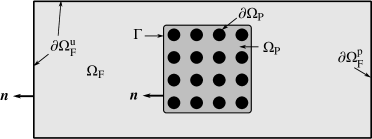
Figure 1: Stokes flow around the bars modeled as a perforated domain.

As a point of departure, consider the Stokes flow over a perforated domain as shown in Fig. 1. We denote, in agreement with Fig. 1, $\Omega_{\mathrm{F}}$ as the reinforcement-free part of the domain and $\Omega_{\mathrm{P}}$ as a part of the domain with the obstacles (further called perforated sub-domain). Boundary of the obstacles is denoted as $\partial\Omega_{\mathrm{P}}$, while the outer boundary $\partial\Omega_{\mathrm{F}}$ is split into two disjoint parts $\partial\Omega_{\mathrm{F}}^{\mathrm{p}}$ and $\partial\Omega_{\mathrm{F}}^{\mathrm{u}}$ corresponding to the type of applied boundary condition; $\Gamma$ stands for the interface between the perforated, $\Omega_{\mathrm{F}}$, and the unperforated, $\Omega_{\mathrm{P}}$, domains. By $\boldsymbol{n}$, we denote both the outer unit normal vector to $\partial\Omega_{\mathrm{F}}$ and $\Gamma$, in the latter case pointed from to $\Omega_{\mathrm{P}}$ to $\Omega_{\mathrm{F}}$.

The governing equations of the steady-state flow of an incompressible fluid in the union of domains $\Omega_{\mathrm{F}}\cup\Omega_{\mathrm{F}}$ take the form

$$-\boldsymbol{\nabla}\cdot\boldsymbol{\tau}\left(\boldsymbol{D}(\boldsymbol{u})\right)+\boldsymbol{\nabla}p=\rho\boldsymbol{b} \Omega_{\mathrm{P}}\cup\Omega_{\mathrm{F}}$$ in (1a)

$$\boldsymbol{\nabla}\cdot\boldsymbol{u}=0 \Omega_{\mathrm{P}}\cup\Omega_{\mathrm{F}}$$ in (1b)

$$\boldsymbol{u}=\boldsymbol{0} \partial\Omega_{\mathrm{P}}$$ in (1c)

$$(\boldsymbol{\tau}-p\boldsymbol{I})\cdot\boldsymbol{n}=-\hat{p}\boldsymbol{n} \partial\Omega_{\mathrm{F}}^{\mathrm{p}}$$ on (1d)

$$\boldsymbol{u}=\hat{u}_{n}\boldsymbol{n} \partial\Omega_{\mathrm{F}}^{\mathrm{u}}$$ on . (1e)

Our notation is standard; $\boldsymbol{\tau}$ stands for the deviatoric part of a stress tensor, the strain rate tensor $\boldsymbol{D}$ is obtained as the symmetrized gradient of the unknown velocity field $\boldsymbol{u}$,

$$\boldsymbol{D}(\boldsymbol{u})=\frac{1}{2}\left(\boldsymbol{\nabla}\boldsymbol{u}+\left(\boldsymbol{\nabla}\boldsymbol{u}\right)^{T}\right),$$

$p$ denotes pressure, $\rho\boldsymbol{b}$ are body forces, $\boldsymbol{I}$ is the unit second order tensor and $\hat{u}_{n}$ and $\hat{p}$ refer to the boundary data. Notice that we set the velocity on the boundary of the bars $\partial\Omega_{\mathrm{P}}$ to zero in (1c). Another physically reasonable possibility is to consider zero velocity in the normal direction to the boundary of the bars only. However, the former case is preferable from the numerical point of view and also it is frequently used by others [27]. We believe that in the most situations it is also more realistic, because in real castings the concrete will stick to the bars during the flow.

2.2 Variational form and two-scale decomposition

The weak form of (1) amounts to finding a pair $(\boldsymbol{u},p)$ such that

$$\int_{\Omega_{\mathrm{P}}}\boldsymbol{\nabla}\boldsymbol{\delta w}:\boldsymbol{\tau}(\boldsymbol{D}(\boldsymbol{u}))\,{\rm d}x-\int_{\Omega_{\mathrm{P}}}(\boldsymbol{\nabla}\cdot\boldsymbol{\delta w})p\,{\rm d}x+\int_{\Omega_{\mathrm{P}}}\delta q(\boldsymbol{\nabla}\cdot\boldsymbol{u})\,{\rm d}x$$ (2a)

$$+\int_{\Omega_{\mathrm{F}}}\boldsymbol{\nabla}\boldsymbol{\delta w}:\boldsymbol{\tau}(\boldsymbol{D}(\boldsymbol{u}))\,{\rm d}x-\int_{\Omega_{\mathrm{F}}}(\boldsymbol{\nabla}\cdot\boldsymbol{\delta w})p\,{\rm d}x+\int_{\Omega_{\mathrm{F}}}\delta q(\boldsymbol{\nabla}\cdot\boldsymbol{u})\,{\rm d}x$$ (2b)

$$+\int_{\partial\Omega_{\mathrm{F}}}\boldsymbol{\delta w}\cdot\hat{p}\boldsymbol{n}\,{\rm d}s+\int_{\Gamma}\llbracket\boldsymbol{\delta w}\cdot\boldsymbol{\tau}\cdot\boldsymbol{n}\rrbracket\,{\rm d}s-\int_{\Gamma}\llbracket\boldsymbol{\delta w}\cdot p\boldsymbol{n}\rrbracket\,{\rm d}s$$ (2c)

$$=\int_{\Omega_{\mathrm{P}}}\boldsymbol{\delta w}\cdot\rho\boldsymbol{b}\,{\rm d}x+\int_{\Omega_{\mathrm{F}}}\boldsymbol{\delta w}\cdot\rho\boldsymbol{b}\,{\rm d}x$$ (2d)

holds for all $(\boldsymbol{\delta w},\delta q)$. Here, (2a), (2b), and (2d) represent the contributions of the perforated and unperforated domains and (2c) appears after the integration by parts. The velocity field $\boldsymbol{u}$ must satisfy the essential boundary conditions (1c) on $\partial\Omega_{\mathrm{P}}$ and (1e) on $\partial\Omega_{\mathrm{F}}^{\mathrm{u}}$, the test field $\boldsymbol{\delta w}=\boldsymbol{0}$ on $\partial\Omega_{\mathrm{P}}$ and on $\partial\Omega_{\mathrm{F}}^{\mathrm{u}}$. In addition, all the involved fields $(\boldsymbol{u},p,\boldsymbol{\delta w},\delta q)$ may be discontinuous across the interface $\Gamma$, which gives rise to the jump terms in (2c) defined as

$$\llbracket f\rrbracket(\boldsymbol{x})=f(\boldsymbol{x})\bigl{|}_{\Omega_{\mathrm{F}}}-f(\boldsymbol{x})\bigl{|}_{\Omega_{\mathrm{P}}}\text{ for }\boldsymbol{x}\in\Gamma,$$

where ${\Omega_{\mathrm{F}}}$ and ${\Omega_{\mathrm{P}}}$ after the vertical line symbolize that the function $f$ is evaluated at the non-perforated or perforated side of the interface $\Gamma$, respectively.

In order to properly average the flow in the perforated domain $\Omega_{\mathrm{P}}$, we follow the idea of the variational multi-scale method by Hughes et al. [29] and its application to porous media by Sandström and Larsson [27] and Sandström et al. [28], and introduce a decomposition of the unknown pressure field $p$ and its corresponding test function $\delta q$ into the macro-scale and sub-scale parts

$$p=p^{\mathrm{M}}+p^{\mathrm{S}},\quad\delta q=\delta q^{\mathrm{M}}+\delta q^{\mathrm{S}}\quad\text{ in }\Omega_{\mathrm{P}}.$$ (3)

We proceed as in [27] by introducing the decomposition (3) into the weak Stokes problem (2) and by integrating the terms containing macro-scale pressure $p^{\mathrm{M}}$ and its corresponding test function $\delta q^{\mathrm{M}}$ by parts. The corresponding parts of (2) then transform into finding $(\boldsymbol{u},p^{\mathrm{M}},p^{\mathrm{S}})$ such that

$$\int_{\Omega_{\mathrm{P}}}\boldsymbol{\nabla}\boldsymbol{\delta w}:\boldsymbol{\tau}(\boldsymbol{D}(\boldsymbol{u}))\,{\rm d}x+\int_{\Omega_{\mathrm{P}}}\boldsymbol{\delta w}\cdot\boldsymbol{\nabla}p^{\mathrm{M}}\,{\rm d}x-\int_{\Omega_{\mathrm{P}}}(\boldsymbol{\nabla}\cdot\boldsymbol{\delta w})p^{\mathrm{S}}\,{\rm d}x$$

$$+\int_{\Gamma}\delta q^{\mathrm{M}}(\boldsymbol{u}\cdot\boldsymbol{n})\,{\rm d}s-\int_{\Omega_{\mathrm{P}}}\boldsymbol{\nabla}\delta q^{\mathrm{M}}\cdot\boldsymbol{u}\,{\rm d}x+\int_{\Omega_{\mathrm{P}}}\delta q^{\mathrm{S}}\boldsymbol{\nabla}\cdot\boldsymbol{u}\,{\rm d}x$$

$$-\int_{\Gamma}\left.\boldsymbol{\delta w}\cdot\boldsymbol{\tau}\right|_{\Omega_{\mathrm{P}}}\cdot\boldsymbol{n}\,{\rm d}s+\int_{\Gamma}\left.\boldsymbol{\delta w}\cdot p^{\mathrm{S}}\right|_{\Omega_{\mathrm{P}}}\boldsymbol{n}\,{\rm d}s$$

$$=\int_{\Omega_{\mathrm{P}}}\boldsymbol{\delta w}\cdot\rho\boldsymbol{b}\,{\rm d}x$$ (4)

$$\int_{\Omega_{\mathrm{P}}}\boldsymbol{\nabla}\boldsymbol{\delta w}:\boldsymbol{\tau}(\boldsymbol{D})\,{\rm d}x-\int_{\Omega_{\mathrm{P}}}(\boldsymbol{\nabla}\cdot\boldsymbol{\delta w})(p^{\mathrm{M}}+p^{\mathrm{S}})\,{\rm d}x+\int_{\Omega_{\mathrm{P}}}(\delta q^{\mathrm{M}}+\delta q^{\mathrm{S}})(\boldsymbol{\nabla}\cdot\boldsymbol{u})\,{\rm d}x$$

$$-\int_{\Gamma}\left.\boldsymbol{\delta w}\cdot\boldsymbol{\tau}\right|_{\Omega_{\mathrm{P}}}\cdot\boldsymbol{n}\,{\rm d}s+\int_{\Gamma}\left.\boldsymbol{\delta w}\cdot(p^{\mathrm{M}}+p^{\mathrm{S}})\right|_{\Omega_{\mathrm{P}}}\boldsymbol{n}\,{\rm d}s$$

$$=\int_{\Omega_{\mathrm{P}}}\boldsymbol{\delta w}\cdot\rho\boldsymbol{b}\,{\rm d}x,$$ (5)

holds for all $(\boldsymbol{\delta w},\delta q^{\mathrm{S}},\delta q^{\mathrm{M}})$, where $\boldsymbol{u}$ and $\boldsymbol{\delta w}$ vanish on the reinforcement boundaries $\partial\Omega_{\mathrm{P}}$, recall Eq. (1c).

2.3 Averaging and pressure extension

The geometry of the perforated domain, Fig. 2, suggests that the domain can be covered by a collection of RVEs $\Omega_{\Box,i}$ with boundary $\partial\Omega_{\Box,i}$, the part of each RVE occupied by fluid is denoted by $\Omega_{\Box,i}^{\mathrm{F}}$ and $\partial\Omega_{\Box,i}^{\mathrm{F}}$ refers to the boundary of the bar. The RVEs adjacent to the internal boundary $\Gamma$ are designated by the index $j$, i.e. $\Omega_{\Box,j}$, and the corresponding parts of their boundaries are denoted by $\Gamma_{\Box,j}$. Finally, $\Omega_{\mathrm{D}}$ refers to the homogenized macro-scale domain covered by RVEs.

Figure 2: Decomposition of the homogenized domain $\Omega_{\mathrm{D}}$ into the union of Representative Volume Elements (RVEs) $\Omega_{\Box,i}$; $\Omega_{\Box,j}$ denotes RVEs adjacent to the fluid domain $\Omega_{\mathrm{F}}$.

Following [27], we define RVE-wise constant volume and boundary averages

$$\left<f\right>(\boldsymbol{x}) =\frac{1}{|\Omega_{\Box,i}^{\mathrm{F}}|}\int_{\Omega_{\Box,i}^{\mathrm{F}}}f\,{\rm d}x\text{ for }\boldsymbol{x}\in\Omega_{\Box,i},$$

$$\left<\left<f\right>\right>(\boldsymbol{x}) =\frac{1}{|\Gamma_{\Box,j}|}\int_{\Gamma_{\Box,j}}f\,{\rm d}s\text{ for }\boldsymbol{x}\in\Gamma_{\Box,j},$$

that satisfy the averaging relation, cf. [27, Section 3.2],

$$\int_{\Omega_{\mathrm{P}}}f\,{\rm d}x=\int_{\Omega_{\mathrm{D}}}\phi\left<f\right>\,{\rm d}x, \int_{\Gamma}f\,{\rm d}x=\int_{\Gamma}\left<\left<f\right>\right>\,{\rm d}x,$$ (6)

where $\phi=|\Omega_{\Box,i}^{\mathrm{F}}|/|\Omega_{\Box,i}|$ denotes the (constant) porosity of the perforated domain. Observe that, in contrast to [27], no coefficient similar to $\phi$ appears in the boundary averaging, because we assume that the obstacles do not intersect the boundary $\Gamma$.

Using (6), the weak formulation (4) can be re-defined over the homogenized domain $\Omega_{\mathrm{D}}$: Find $(\boldsymbol{u},p^{\mathrm{M}},p^{\mathrm{S}})$ such that

$$\int_{\Gamma}\left<\left<\delta q^{\mathrm{M}}(\boldsymbol{u}\cdot\boldsymbol{n})\right>\right>\,{\rm d}s-\int_{\Omega_{\mathrm{D}}}\phi\left<\boldsymbol{\nabla}\delta q^{\mathrm{M}}\cdot\boldsymbol{u}\right>\,{\rm d}x$$ (7a)

$$+ \int_{\Omega_{\mathrm{D}}}\phi\left<\delta q^{\mathrm{S}}\boldsymbol{\nabla}\cdot\boldsymbol{u}\right>\,{\rm d}x+\int_{\Omega_{\mathrm{D}}}\phi\left<\boldsymbol{\nabla}\boldsymbol{\delta w}:\boldsymbol{\tau}(\boldsymbol{D}(\boldsymbol{u}))\right>\,{\rm d}x$$

$$+ \int_{\Omega_{\mathrm{D}}}\phi\left<\boldsymbol{\delta w}\cdot\boldsymbol{\nabla}p^{\mathrm{M}}\right>\,{\rm d}x-\int_{\Omega_{\mathrm{D}}}\phi\left<(\boldsymbol{\nabla}\cdot\boldsymbol{\delta w})p^{\mathrm{S}}\right>\,{\rm d}x$$ (7b)

$$- \int_{\Gamma}\left<\left<\boldsymbol{\delta w}\cdot\boldsymbol{\tau}\bigl{|}_{\Omega_{\mathrm{P}}}\cdot\boldsymbol{n}\right>\right>\,{\rm d}s+\int_{\Gamma}\left.\left<\left<\boldsymbol{\delta w}\cdot p^{\mathrm{S}}\right|_{\Omega_{\mathrm{P}}}\boldsymbol{n}\right>\right>\,{\rm d}s$$ (7c)

$$= \int_{\Omega_{\mathrm{D}}}\phi\left<\boldsymbol{\delta w}\cdot\rho\boldsymbol{b}\right>\,{\rm d}x$$ (7d)

holds for all $(\boldsymbol{\delta w},\delta q^{\mathrm{S}},\delta q^{\mathrm{M}})$.

As customary in conventional homogenization theories, we assume that the RVEs $\Omega_{\Box,i}$ are much smaller than the homogenized domain $\Omega_{\mathrm{D}}$, so that the contribution of the boundary terms (7c) to (7) is negligible. To clarify this assumption, consider a sub-scale traction vector

$$\boldsymbol{T}^{\mathrm{S}}=(\boldsymbol{\tau}-p^{\mathrm{S}}\boldsymbol{I})\cdot\boldsymbol{n},$$ (8)

associated with the stress tensor $\boldsymbol{\tau}$ and the sub-scale pressure $p^{\mathrm{S}}$. Neglecting (7c) thus means neglecting the virtual work of the sub-scale tractions at the whole boundary $\Gamma$,

$$\int_{\Gamma}\left<\left<\boldsymbol{\delta w}\cdot\boldsymbol{T}^{\mathrm{S}}\bigl{|}_{\Omega_{\mathrm{P}}}\right>\right>\,{\rm d}s\approx 0.$$

We shall see later in Section 2.5 that this contribution is partially compensated for by the interface conditions between the reinforcement-free and homogenized domains.

The transition from the perforated domain $\Omega_{\mathrm{P}}$ to the homogenized domain $\Omega_{\mathrm{D}}$ is completed by extending the macro-scale pressure $p^{\mathrm{M}}$ (defined on $\Omega_{\mathrm{P}}$) to a smooth pressure field $\bar{p}$ (defined on the whole $\Omega_{\mathrm{D}}$), which satisfies the matching conditions

$$\bar{p}(\bar{\boldsymbol{x}}_{i})=\left<p^{\mathrm{M}}\right>(\bar{\boldsymbol{x}}_{i}), \boldsymbol{\nabla}\bar{p}(\bar{\boldsymbol{x}}_{i})=\left<\boldsymbol{\nabla}p^{\mathrm{M}}\right>(\bar{\boldsymbol{x}}_{i}),$$

at the center of the $i$-th RVE $\bar{\boldsymbol{x}}_{i}$, recall Fig. 2. By analogy, we also extend the test function $\delta q^{\mathrm{M}}$ to $\delta\bar{q}$, from $\Omega_{\mathrm{P}}$ to $\Omega_{\mathrm{D}}$.

2.4 First-order homogenization

Now, we adopt the ansatz of the first-order homogenization, and expand the unknown fields in each RVE into an affine part macro-scale and a periodic sub-scale correction, cf. [39, 40, 27]. The resulting approximations at $\boldsymbol{x}\in\Omega_{\Box,i}^{\mathrm{F}}$ take the form

$$p(\boldsymbol{x}) \approx(p^{\mathrm{M}}+p^{\mathrm{S}})(\boldsymbol{x})=\bar{p}(\bar{\boldsymbol{x}}_{i})+\boldsymbol{\nabla}\bar{p}(\bar{\boldsymbol{x}}_{i})\cdot(\boldsymbol{x}-\bar{\boldsymbol{x}}_{i})+p^{\mathrm{S}}(\boldsymbol{x}),$$ (9a)

$$\boldsymbol{u}(\boldsymbol{x}) \approx\boldsymbol{u}^{\mathrm{S}}(\boldsymbol{x}),$$ (9b)

where

$$p^{\mathrm{S}}\text{ is periodic on }\partial\Omega_{\Box,i}, \left<p^{\mathrm{S}}\right> =0\text{ in }\Omega_{\Box,i},$$

$$\boldsymbol{u}^{\mathrm{S}}\text{ is periodic on }\partial\Omega_{\Box,i}, \boldsymbol{u}^{\mathrm{S}} =\boldsymbol{0}\text{ on }\partial\Omega_{\Box,i}^{\mathrm{F}}.$$

A similar expansion is adopted for the test functions

$$\delta q(\boldsymbol{x}) \approx(\delta q^{\mathrm{M}}+\delta q^{\mathrm{S}})(\boldsymbol{x})=\delta\bar{q}(\bar{\boldsymbol{x}}_{i})+\boldsymbol{\nabla}\delta\bar{q}(\bar{\boldsymbol{x}}_{i})\cdot(\boldsymbol{x}-\bar{\boldsymbol{x}}_{i})+\delta q^{\mathrm{S}}(\boldsymbol{x}),$$ (11a)

$$\boldsymbol{\delta w}(\boldsymbol{x}) \approx\boldsymbol{\delta w}^{\mathrm{S}}(\boldsymbol{x}),\text{ for }\boldsymbol{x}\in\Omega_{\Box,i}^{\mathrm{F}},$$ (11b)

with the test fields $(\delta q^{\mathrm{S}},\boldsymbol{\delta w}^{\mathrm{S}})$ satisfying the same conditions as the pair $(p^{\mathrm{S}},\boldsymbol{u}^{\mathrm{S}})$ in (10).

We now proceed with testing the weak form (7) separately with the macro-scale, Section 2.4.1, and micro-scale, Section 2.4.2, test functions, from which we extract the corresponding macro- and micro-scale problems of the Darcy and the Stokes type, respectively.

2.4.1 Macro-scale Darcy law

Inserting the expansion of the macro-scale pressure test function (11a) into (7a) gives rise to the terms, cf. [27, Eq. (15)]

$$\int_{\Omega_{\mathrm{D}}}\phi\left<\boldsymbol{\nabla}\delta q^{\mathrm{M}}\cdot\boldsymbol{u}\right>\,{\rm d}x \approx\int_{\Omega_{\mathrm{D}}}\boldsymbol{\nabla}\delta{\bar{q}}\cdot\phi\left<\boldsymbol{u}\right>\,{\rm d}x,$$

$$\int_{\Gamma}\left<\left<\delta q^{\mathrm{M}}(\boldsymbol{u}\cdot\boldsymbol{n})\right>\right>\,{\rm d}s \approx\int_{\Gamma}\delta\bar{q}\left<\left<\boldsymbol{u}\right>\right>\cdot\boldsymbol{n}\,{\rm d}s.$$

By introducing the seepage velocity via

$$\bar{\boldsymbol{u}}=\phi\left<\boldsymbol{u}\right>\text{ in }\Omega_{\mathrm{D}}, \bar{\boldsymbol{u}}=\left<\left<\boldsymbol{u}\right>\right>\text{ on }\Gamma,$$

we finally see that (7a) encodes the weak from of the mass conservation condition

$$\int_{\Omega_{\mathrm{D}}}\boldsymbol{\nabla}\delta\bar{q}\cdot\bar{\boldsymbol{u}}\,{\rm d}x=\int_{\Gamma}\delta\bar{q}\bar{\boldsymbol{u}}\cdot\boldsymbol{n}\,{\rm d}s.$$

For numerical convenience, and also for purpose of coupling the homogenized flow in $\Omega_{\mathrm{D}}$ to the flow in the fluid domain $\Omega_{\mathrm{F}}$, we further express the conservation condition in an equivalent form

$$\int_{\Omega_{\mathrm{D}}}\delta\bar{q}(\boldsymbol{\nabla}\cdot\bar{\boldsymbol{u}})\,{\rm d}x=0,$$ (12)

To complete the macro-scale problem, in the next section we will show that the seepage velocity is driven by macro-scale gradient $\boldsymbol{\nabla}\bar{p}$ and by the body forces $\rho\boldsymbol{b}$,

$$\bar{\boldsymbol{u}}=\boldsymbol{\bar{w}}(\boldsymbol{\nabla}\bar{p},\rho\boldsymbol{b})\text{ in }\Omega_{\mathrm{D}},$$ (13)

so that (12) and (13) indeed represent a non-linear Darcian flow in $\Omega_{\mathrm{D}}$.

2.4.2 Micro-scale Stokes problem

The sub-scale problem is obtained from (7b) and (7d) by localizing the test functions to individual RVEs $\Omega_{\Box,i}$ according to (11). Abbreviating $\bar{\boldsymbol{g}}=\boldsymbol{\nabla}\bar{p}(\bar{\boldsymbol{x}}_{i})$, the resulting problem reads as follows: Find $(\boldsymbol{u}^{\mathrm{S}},p^{\mathrm{S}})$ such that

$$\int_{\Omega_{\Box,i}^{\mathrm{F}}}\boldsymbol{\nabla}\boldsymbol{\delta w}^{\mathrm{S}}:\boldsymbol{\tau}(\boldsymbol{D}(\boldsymbol{u}^{\mathrm{S}}))\,{\rm d}x-\int_{\Omega_{\Box,i}^{\mathrm{F}}}(\boldsymbol{\nabla}\cdot\boldsymbol{\delta w}^{\mathrm{S}})p^{\mathrm{S}}\,{\rm d}x =\int_{\Omega_{\Box,i}^{\mathrm{F}}}\boldsymbol{\delta w}^{\mathrm{S}}\cdot\left(\rho\boldsymbol{b}-\bar{\boldsymbol{g}}\right)\,{\rm d}x,$$ (14a)

$$\int_{\Omega_{\Box,i}^{\mathrm{F}}}\delta q^{\mathrm{S}}(\boldsymbol{\nabla}\cdot\boldsymbol{u}^{\mathrm{S}})\,{\rm d}x =0,$$ (14b)

hold for all $(\boldsymbol{\delta w}^{\mathrm{S}},\delta q^{\mathrm{S}})$, where both $(\boldsymbol{u}^{\mathrm{S}},p^{\mathrm{S}})$ and $(\boldsymbol{\delta w}^{\mathrm{S}},\delta q^{\mathrm{S}})$ satisfy (10). This problem implicitly defines the sub-scale velocity $\boldsymbol{u}^{\mathrm{S}}$ as a function of the macro-scale pressure $\bar{\boldsymbol{g}}$ and the body force $\rho\boldsymbol{b}$, postulated formally in (13).

Finally let us remark that (14a) does not contain the boundary contributions

$$\int_{\partial\Omega_{\Box,i}}\boldsymbol{\delta w}^{\mathrm{S}}\cdot\boldsymbol{T},$$

where $\boldsymbol{T}$, in analogy to (8), denotes the tractions at the RVE boundary associated with the stress $\boldsymbol{\tau}$ and pressure $p$ from (9a). As shown in [27, Eq. (32)], this term vanishes as a consequence of the periodicity enforced in (10).

2.5 Stokes-Darcy coupling

A closer inspection reveals that the only terms in (2) remaining for further considerations are

$$\int_{\Gamma}\left.\boldsymbol{\delta w}\cdot\boldsymbol{\tau}\right|_{\Omega_{\mathrm{F}}}\cdot\boldsymbol{n}\,{\rm d}s-\int_{\Gamma}\left.\boldsymbol{\delta w}\cdot p\right|_{\Omega_{\mathrm{F}}}\cdot\boldsymbol{n}\,{\rm d}s;$$ (15)

recall Eq. (2c) in particular. This contribution is made explicit by imposing the interface conditions between Darcy and Stokes sub-domains in the form

$$u_{n}-\bar{u}_{n} =0 \text{on }\Gamma,$$ (16a)

$$p-\bar{p} =\boldsymbol{n}\cdot\boldsymbol{\tau}\cdot\boldsymbol{n} \text{on }\Gamma,$$ (16b)

$$\beta\left(u_{t}-\bar{u}_{t}\right) =\boldsymbol{t}\cdot\boldsymbol{\tau}\cdot\boldsymbol{n} \text{on }\Gamma,$$ (16c)

where $\boldsymbol{n}$ and $\boldsymbol{t}$ denote the unit vectors normal to and tangent to $\Gamma$, respectively, see Fig. 3, and where we have utilized the decompositions of the fluid, $\boldsymbol{u}$, and seepage, $\bar{\boldsymbol{u}}$, velocities into the components normal and tangential to $\Gamma$,

$$\boldsymbol{u}=u_{n}\boldsymbol{n}+u_{t}\boldsymbol{t}, \bar{\boldsymbol{u}}=\bar{u}_{n}\boldsymbol{n}+\bar{u}_{t}\boldsymbol{t} \text{on }\Gamma;$$ (17)

notice that in (16b) and (16c) we omitted the symbol $\bigl{|}_{\Omega_{\mathrm{F}}}$ to keep the notation simple. Eq. (16b) thus represents the continuity of velocity in the normal direction, (16a) enforces the equilibrium condition in the normal direction, and (16c) is the Beavers-Joseph-Saffman (BJS) slip law [30, 31] involving the interface constant $\beta$. As was shown by Saffman [31], the tangential velocities satisfy $\bar{u}_{t}\ll u_{t}$, so that we set

$$\overline{u}_{t}=0\text{ on }\Gamma.$$ (18)

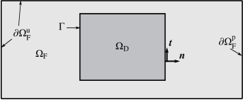
Figure 3: Description of the Stokes-Darcy problem

Utilizing the decomposition (17) also for the test functions $\boldsymbol{\delta w}$, the terms in (15) expand into

$$\int_{\Gamma}\delta w_{t}\boldsymbol{t}\cdot\boldsymbol{\tau}\cdot\boldsymbol{n}\,{\rm d}s+\int_{\Gamma}\delta w_{n}\boldsymbol{n}\cdot\boldsymbol{\tau}\cdot\boldsymbol{n}\,{\rm d}s-\int_{\Gamma}\delta w_{n}p\,{\rm d}s =$$

$$\int_{\Gamma}\delta w_{t}\beta\left(u_{t}-\bar{u}_{t}\right)\,{\rm d}s+\int_{\Gamma}\delta w_{n}(p-\bar{p})\,{\rm d}s-\int_{\Gamma}\delta w_{n}p\,{\rm d}s =$$

$$\int_{\Gamma}\delta w_{t}\beta u_{t}\,{\rm d}s-\int_{\Gamma}\delta w_{n}\bar{p}\,{\rm d}s.$$ (19)

As follows from analytical results by Jäger and Mikelić [32] and numerical studies by Jäger et al. [33] and Carraro et al. [34], parameter $\beta$ governing the friction in (16b) for Newtonian fluids can be expressed as

$$\beta=-\frac{\mu}{C^{\mathrm{bl}}},$$ (20)

where $\mu$ is viscosity of the fluid, cf. 28, and $C^{\mathrm{bl}}$ is determined from the solution of a boundary layer problem defined for RVEs in the vicinity of the internal boundary $\Gamma$, as shown in Fig. 4.

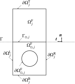
Figure 4: Scheme of the boundary layer problem.

In our notation, the problem reads as: Find $(\boldsymbol{u}^{\mathrm{S}},p^{\mathrm{S}})$ such that

$$\int_{\Omega^{\mathrm{F}}_{\Box,j}\cup\Omega^{\mathrm{F}}_{j}}\boldsymbol{\nabla}\boldsymbol{\delta w}^{\mathrm{S}}:\boldsymbol{\nabla}\boldsymbol{u}^{\mathrm{S}}\,{\rm d}x-\int_{\Omega^{\mathrm{F}}_{\Box,j}\cup\Omega^{\mathrm{F}}_{j}}(\boldsymbol{\nabla}\cdot\boldsymbol{\delta w}^{\mathrm{S}})p^{\mathrm{S}}\,{\rm d}x$$

$$+ \int_{\Omega^{\mathrm{F}}_{\Box,j}\cup\Omega^{\mathrm{F}}_{j}}\delta q^{\mathrm{S}}(\boldsymbol{\nabla}\cdot\boldsymbol{\delta w}^{\mathrm{S}})\,{\rm d}x=0$$

holds for all $(\boldsymbol{\delta w}^{\mathrm{S}},\delta q^{\mathrm{S}})$. All fields above are periodic at $\partial\Omega_{j}^{\mathrm{L}}$ and $\partial\Omega_{j}^{\mathrm{R}}$, and satify in addition $\boldsymbol{\delta w}^{\mathrm{S}}=\boldsymbol{u}^{\mathrm{S}}=\boldsymbol{0}$ on $\partial\Omega_{\Box,j}^{\mathrm{F}}$ and $\partial\Omega_{j}^{\mathrm{B}}$, $\delta w_{t}^{\mathrm{S}}=u_{t}^{\mathrm{S}}=0$ on $\partial\Omega_{j}^{\mathrm{T}}$, $\boldsymbol{\delta w}^{\mathrm{S}}=\boldsymbol{u}^{\mathrm{S}}=\boldsymbol{0}$ on $\Gamma_{\Box,j}$, $\llbracket\boldsymbol{\delta w}^{\mathrm{S}}\rrbracket=\llbracket\boldsymbol{u}^{\mathrm{S}}\rrbracket=\boldsymbol{0}$ on $\Gamma_{\Box,j}$, and

$$\int_{\Gamma_{\Box,j}}\delta q^{\mathrm{S}}\,{\rm d}s=\int_{\Gamma_{\Box,j}}p^{\mathrm{S}}\,{\rm d}s=0.$$

The interface constant $C^{\mathrm{bl}}$ is then obtained as

$$C^{\mathrm{bl}}=\int_{\Gamma_{\Box,j}}u^{\mathrm{S}}_{t}\,{\rm d}s,$$ (21)

and therefore depends only on the geometry of perforations. To the best of our knowledge, no extension of these results to non-linear fluids is currently available.

2.6 Darcy-Stokes system

Collecting the results of the previous Sections 2.2–2.5, we recast the original weak formulation (2) into the final form: Find a quadruple $(\boldsymbol{u},\bar{\boldsymbol{u}},p,\bar{p})$ such that

$$\int_{\Omega_{\mathrm{D}}}\delta\bar{q}(\boldsymbol{\nabla}\cdot\bar{\boldsymbol{u}})\,{\rm d}x+\int_{\Omega_{\mathrm{D}}}\boldsymbol{\delta\bar{w}}\cdot\bar{\boldsymbol{u}}\,{\rm d}x-\int_{\Omega_{\mathrm{D}}}\boldsymbol{\delta\bar{w}}\cdot\boldsymbol{\bar{w}}(\boldsymbol{\nabla}\bar{p},\rho\boldsymbol{b})\,{\rm d}x$$

$$+ \int_{\Omega_{\mathrm{F}}}\boldsymbol{\nabla}\boldsymbol{\delta w}:\boldsymbol{\tau}(\boldsymbol{D}(\boldsymbol{u}))\,{\rm d}x-\int_{\Omega_{\mathrm{F}}}(\boldsymbol{\nabla}\cdot\boldsymbol{\delta w})p\,{\rm d}x+\int_{\Omega_{\mathrm{F}}}\delta q(\boldsymbol{\nabla}\cdot\boldsymbol{u})\,{\rm d}x$$

$$+ \int_{\partial\Omega_{\mathrm{F}}^{\mathrm{p}}}\delta w_{n}\hat{p}\,{\rm d}s+\int_{\Gamma}\delta w_{t}\beta u_{t}\,{\rm d}s-\int_{\Gamma}\delta w_{n}\bar{p}\,{\rm d}s$$

$$= \int_{\Omega_{\mathrm{F}}}\boldsymbol{\delta w}\cdot\rho\boldsymbol{b}\,{\rm d}x$$ (22)

for all $(\boldsymbol{\delta w},\boldsymbol{\delta\bar{w}},\delta q,\delta\overline{q})$, where $(\boldsymbol{u},\boldsymbol{\delta w})=(\hat{u}_{n}\boldsymbol{n},\boldsymbol{0})$ on $\partial\Omega_{\mathrm{F}}^{\mathrm{u}}$ according to (1e), $\bar{u}_{t}=\delta\bar{w}_{t}=0$ on $\Gamma$ according to (18), and $\bar{u}_{n}=u_{n}$ and $\delta\bar{w}_{n}=\delta w_{n}$ on $\Gamma$ by (16a), cf. Fig. 3.

3 Numerical solution

Notice that the problem (22) is non-linear, because of possible non-linearity of the constitutive laws $\boldsymbol{\tau}(\boldsymbol{D}(\boldsymbol{u}))$ and consequently of $\boldsymbol{\bar{w}}(\boldsymbol{\nabla}\bar{p},\rho\boldsymbol{b})$, and as such it is treated using successive consistent linearization introduced in Section 3.1. The finite element discretization of the ensuing linear system and the implementation of a Newton solver are outlined in Section 3.2.

3.1 Linearization

In order to avoid a profusion of notation, we denote still by $(\boldsymbol{u},\bar{\boldsymbol{u}},p,\bar{p})$ the solution around which the linearization is performed. Its iterative correction $(\boldsymbol{v},\bar{\boldsymbol{v}},q,\bar{q})$ is defined by the associated linear problem, cf. (22):

$$\underbrace{\int_{\Omega_{\mathrm{D}}}\delta\bar{q}(\boldsymbol{\nabla}\cdot\bar{\boldsymbol{v}})\,{\rm d}x}_{\bar{G}}+\underbrace{\int_{\Omega_{\mathrm{D}}}\boldsymbol{\boldsymbol{\delta\bar{w}}}\cdot\bar{\boldsymbol{v}}\,{\rm d}x}_{\bar{M}}-\underbrace{\int_{\Omega_{\mathrm{D}}}\boldsymbol{\boldsymbol{\delta\bar{w}}}\cdot\frac{\partial\boldsymbol{\bar{w}}(\boldsymbol{\nabla}\bar{p},\rho\boldsymbol{b})}{\partial\boldsymbol{\nabla}\bar{p}}\cdot\boldsymbol{\nabla}\bar{q}\,{\rm d}x}_{\bar{K}_{t}}$$

$$+ \underbrace{\int_{\Omega_{\mathrm{F}}}\boldsymbol{\nabla}\boldsymbol{\delta w}:\frac{\partial\boldsymbol{\tau}(\boldsymbol{D})}{\partial\boldsymbol{\nabla}\boldsymbol{u}}:\boldsymbol{\nabla}\boldsymbol{v}\,{\rm d}x}_{K_{t}}-\underbrace{\int_{\Omega_{\mathrm{F}}}(\boldsymbol{\nabla}\cdot\boldsymbol{\delta w})q\,{\rm d}x}_{G_{p}}+\underbrace{\int_{\Omega_{\mathrm{F}}}\delta q(\boldsymbol{\nabla}\cdot\boldsymbol{v})\,{\rm d}x}_{G_{u}}$$

$$+\underbrace{\int_{\Gamma}\delta w_{t}\beta v_{t}\,{\rm d}s}_{M_{\Gamma}}-\underbrace{\int_{\Gamma}\delta w_{n}\bar{q}\,{\rm d}s}_{G_{\Gamma}}$$

$$=$$ (23)

$$- \underbrace{\int_{\Omega_{\mathrm{D}}}\delta\bar{q}(\boldsymbol{\nabla}\cdot\bar{\boldsymbol{u}})\,{\rm d}x}_{\bar{f}_{q}}-\underbrace{\int_{\Omega_{\mathrm{D}}}\boldsymbol{\boldsymbol{\delta\bar{w}}}\cdot\bar{\boldsymbol{u}}\,{\rm d}x}_{\bar{f}_{u}}+\underbrace{\int_{\Omega_{\mathrm{D}}}\boldsymbol{\boldsymbol{\delta\bar{w}}}\cdot\boldsymbol{\bar{w}}(\boldsymbol{\nabla}\bar{p},\rho\boldsymbol{b})\,{\rm d}x}_{\bar{f}_{w}}$$

$$-\underbrace{\int_{\Omega_{\mathrm{F}}}\boldsymbol{\nabla}\boldsymbol{\delta w}:\boldsymbol{\tau}(\boldsymbol{D})\,{\rm d}x}_{f_{\tau}}+\underbrace{\int_{\Omega_{\mathrm{F}}}(\boldsymbol{\nabla}\cdot\boldsymbol{\delta w})p\,{\rm d}x}_{f_{p}}-\underbrace{\int_{\Omega_{\mathrm{F}}}\delta q(\boldsymbol{\nabla}\cdot\boldsymbol{u})\,{\rm d}x}_{f_{q}}$$

$$-\underbrace{\int_{\Gamma}\delta w_{t}\beta u_{t}\,{\rm d}s}_{f_{f}}+\underbrace{\int_{\Gamma}\delta w_{n}\bar{p}\,{\rm d}s}_{f_{\Gamma}}+\underbrace{\int_{\Omega_{\mathrm{F}}}\boldsymbol{\delta w}\cdot\rho\boldsymbol{b}\,{\rm d}x}_{f_{b}}+\underbrace{\int_{\partial\Omega_{\mathrm{F}}^{\mathrm{p}}}\delta w_{n}\hat{p}\,{\rm d}s}_{f_{t}},$$

where $\boldsymbol{v}=\boldsymbol{0}$ on $\partial\Omega_{\mathrm{F}}^{\mathrm{u}}$, and the seepage velocity $\bar{\boldsymbol{v}}$ and the test functions $(\boldsymbol{\delta w},\boldsymbol{\delta}\bar{\boldsymbol{w}},\delta q,\delta\bar{q})$ satisfy the same conditions as in the non-linear problem in (22).

The linearization is finalized by evaluating the sensitivities of the local constitutive laws. In the Stokes domain, the application of the chain rule gives

$$\frac{\partial\boldsymbol{\tau}(\boldsymbol{D})}{\partial(\boldsymbol{\nabla}\boldsymbol{u})}=\frac{\partial\boldsymbol{\tau}(\boldsymbol{D})}{\partial\boldsymbol{D}}:\frac{\partial\boldsymbol{D}}{\partial(\boldsymbol{\nabla}\boldsymbol{u})}=\frac{\partial\boldsymbol{\tau}(\boldsymbol{D})}{\partial\boldsymbol{D}}:\boldsymbol{\mathcal{I}_{dev}},$$ (24)

where the specific form of the derivative $\frac{\partial\tau(\boldsymbol{D})}{\partial\boldsymbol{D}}$ depends on the particular choice of constitutive law and $\boldsymbol{\mathcal{I}_{dev}}$ is the deviatoric projector defined as

$$[\boldsymbol{\mathcal{I}_{dev}}]_{ijkl}=\delta_{ik}\delta_{jl}-\frac{1}{3}\delta_{ij}\delta_{kl}.$$ (25)

In the homogenized Darcy domain, it holds [27, Section 5]

$$\frac{\partial\boldsymbol{\bar{w}}(\boldsymbol{\nabla}\bar{p},\rho\boldsymbol{b})}{\partial\boldsymbol{\nabla}\bar{p}}=\phi\sum_{k=1}^{2}\left<\boldsymbol{u}^{\mathrm{S}}_{(k)}\right>\otimes\boldsymbol{e}_{(k)},$$ (26)

where $\boldsymbol{u}^{\mathrm{S}}_{(k)}$ denotes the solution to the linearized sub-scale problem (14) with the macroscopic pressure gradient $\bar{\boldsymbol{g}}$ set to the $k$-th canonical basis vector $\boldsymbol{e}_{(k)}$.

3.2 Finite element treatment

The linearized weak form can now be discretized using conventional finite element procedures. At the element level, Eq. (23) is recast into the equivalent matrix form

$$\begin{pmatrix}\boldsymbol{K}_{t}+\boldsymbol{M}_{\Gamma}+\bar{\boldsymbol{M}}&\bar{\boldsymbol{K}}_{t}+\boldsymbol{G}_{\Gamma}+\boldsymbol{G}_{p}\\ \boldsymbol{G}_{u}+\bar{\boldsymbol{G}}&\boldsymbol{0}_{3\times 3}\end{pmatrix}\begin{Bmatrix}\boldsymbol{v}\\ \boldsymbol{q}\end{Bmatrix}=\begin{Bmatrix}\boldsymbol{f}_{ext,u}-\boldsymbol{f}_{int,u}\\ -\boldsymbol{f}_{int,p}\end{Bmatrix},$$ (27)

where the individual terms contain contribution from in the Darcy domain $\Omega_{\mathrm{D}}$, the Stokes domain $\Omega_{\mathrm{F}}$, at the internal interface $\Gamma$, or at the boundary $\Gamma_{\mathrm{P}}$, in accordance with (23). The vector on the right hand side consists of sub-vectors defined as

$$\boldsymbol{f}_{ext,u}=\boldsymbol{f}_{t}+\boldsymbol{f}_{b},$$

$$\boldsymbol{f}_{int,u}=\bar{\boldsymbol{f}}_{q}+\bar{\boldsymbol{f}}_{u}-\bar{\boldsymbol{f}}_{w}+\boldsymbol{f}_{\tau}-\boldsymbol{f}_{p}+\boldsymbol{f}_{f}-\boldsymbol{f}_{\Gamma},\qquad\boldsymbol{f}_{int,p}=\boldsymbol{f}_{q}$$

Notice the $3\times 3$ null sub-matrix in (27) which may cause numerical problems, if spaces of approximation functions do not satisfy the so-called inf-sup condition [41, 42]. For this reason, we employed the Taylor-Hood $P2/P1$ elements with the quadratic approximation of velocity and the linear approximation of pressure. Depending on the order of the polynomial in individual terms, 3 or 7 integration points were used. The sub-scale problem (14) is treated in the same fashion. The permeability matrix (26) is being kept constant for each one element inside the Darcy Domain, i.e. the sub-scale problem is solved only once (in one integration point) for each Darcy element.

At the structural level, we use the Newton method with a back-tracking line search to ensure a robust convergence with the quadratic rate. In particular, we used the backtracking algorithm introduced in [43, Section 7.2.3, Program 62], with the decrease parameter $\sigma=10^{-4}$ and with the scaling factor $\rho=0.5$. The outlined solution procedure was implemented into OOFEM code [44, 45].

4 Examples

In this section, two benchmark tests are presented to illustrate the capabilities and performance of the proposed method. The first example, Fig. 5, illustrates unidirectional flow of a fluid around reinforcing bars. The second example, Fig. 8, is more complex and illustrates the complex flow of the concrete over the reinforced area with a significant effect of the friction interface parameter $\beta$, recall Eq. (16c). In both examples, the solution based on the homogenization technique is verified against a fully resolved solution computed by Direct Numerical Simulation (DNS).

We will consider two constitutive laws: Newtonian fluids with viscosity $\mu$,

$$\boldsymbol{\tau}=\mu\boldsymbol{D},$$ (28)

and a regularized Bingham model [46] defined as

$$\boldsymbol{\tau}=\left[\mu_{0}+\frac{\tau_{0}}{\sqrt{J_{2}^{D}}}\left(1-\exp(-m\sqrt{J_{2}^{D}})\right)\right]\boldsymbol{D},$$ (29)

where $\tau_{0}$ is the yield stress, representing an initial resistance to the flow, $\mu_{0}$ is the plastic viscosity, which governs the flow once the yield stress threshold has been passed, and $m$ is the regularization parameter. The second invariant of the deviatoric strain tensor $J_{2}^{D}$ is defined as

$$J_{2}^{D}=\frac{1}{2}\boldsymbol{D}:\boldsymbol{D},$$

The constitutive tangents, needed in (24), are thus provided by

$$\frac{\partial\boldsymbol{\tau}(\boldsymbol{D})}{\partial\boldsymbol{D}} =\mu_{\mathrm{app}}(\boldsymbol{D})\boldsymbol{\mathcal{I}}_{\mathrm{sym}}+\mu^{\prime}_{\mathrm{app}}(\boldsymbol{D})\boldsymbol{D}\otimes\boldsymbol{D},$$ (30)

where $\boldsymbol{\mathcal{I}}_{\mathrm{sym}}$ is the unit fourth order tensor with both major and minor symmetries, and the apparent viscosity $\mu_{\mathrm{app}}$ and its derivative $\mu^{\prime}_{\mathrm{app}}$ are provided by

$$\mu_{\mathrm{app}}(\boldsymbol{D}) =\mu_{0}+\frac{\tau_{0}}{\sqrt{J_{2}^{D}}}\left(1-\exp(-m\sqrt{J_{2}^{D}})\right),$$

$$\mu^{\prime}_{\mathrm{app}}(\boldsymbol{D}) =\frac{\left[\left(m\sqrt{J_{2}^{D}}+1\right)\exp\left(-m\sqrt{J_{2}^{D}}\right)-1\right]\tau_{0}}{2(J_{2}^{D})^{\frac{3}{2}}}.$$

In what follows, all quantities will be expressed in consistent units.

We also wish to emphasize that both examples involve an array of only $4\times 4$ RVEs of unit length with the obstacle radius of $\xi$, so that macro and micro length scales are not widely separated. This setup is, therefore, quite unfavorable for the multi-scale method, but our results show that it still corresponds well with DNS. Even higher accuracy is expected for an increasing length scale contrast.

4.1 Unidirectional flow

The setup of this benchmark test is shown in Fig. 5. The flow is driven by constant velocity in the normal direction, prescribed on the left edge of the domain. The top and the bottom edges are friction-free and the “do nothing” boundary condition is prescribed on the right edge. The Newton fluid of the unit viscosity, $\mu=1$, is considered in this elementary example and the radius of bars is taken as $\xi=0.25$. The friction parameter $\beta$ is set to $1$ on the Stokes side of the interface, but it does not play any important role in this case, as the flow is perpendicular to the interface. Computational meshes for both fully resolved and homogenized cases are shown in Fig. 6.

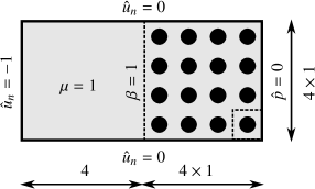
Figure 5: Unidirectional flow: scheme of the benchmark test.

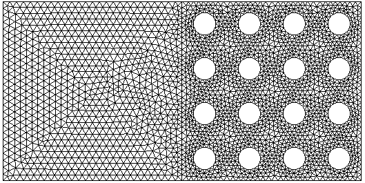
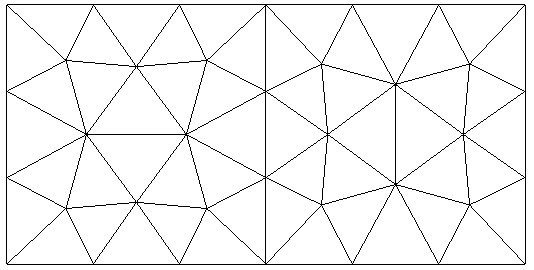
Figure 6: Unidirectional flow: comparison of the meshes. Mesh for fully resolved problem (left - $11,358$ nodes, $5,004$ quadratic elements) and for homogenized problem (right - $130$ nodes, $52$ quadratic elements).

In Fig. 7, the results obtained from the homogenized formulation (left) and the fully resolved solution (right) are presented. The pressure contours are shown in the background, while the velocity field is visualized using arrows in nodal points. Notice that the velocity field in the homogenized solution is uniform and equal to the prescribed boundary condition due to the incompressibility constraint, as the fluid cannot flow elsewhere but through the reinforced domain. The pressure distributions are in very good agreement; the error in the $\max$ norm is approximately $10\%$.

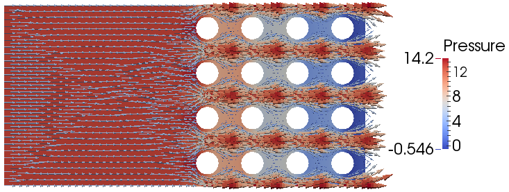
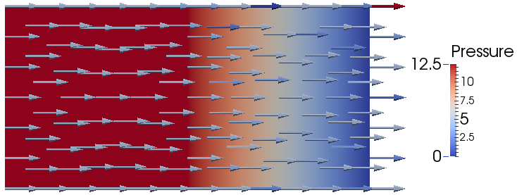
Figure 7: Unidirectional flow: comparison of fully resolved solution (left) and homogenized solution (right).

4.2 Flow over reinforced area

The second example illustrates the more complex flow pattern around the reinforced domain. The reinforced area is located in the middle of the problem domain, so the fluid is not forced to go through the reinforcing bars and the whole situation is closer to real casting problems. This problem also allows us to study the influence of the friction parameter $\beta$. The test is considered in two variations. In the first variant, the geometry of the reinforced area is parallel to the direction of the prescribed flow, while in the second case, the geometry of the reinforced area is rotated with respect to the prescribed flow direction. The schematic setup of both situations is outlined in Fig. 8. Again, uniform velocity is prescribed on the left side, no friction on the top and the bottom and zero “do nothing” boundary condition on the right. The RVEs are chosen with $\xi=0.125$, $\xi=0.25$, and $\xi=0.35$.

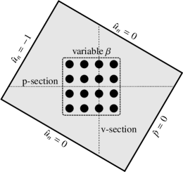
Figure 8: Flow over reinforced area: scheme of the benchmark test.

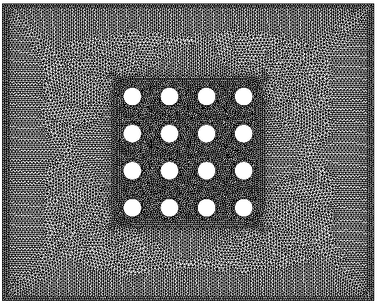
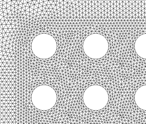
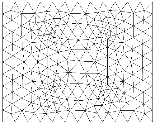
Figure 9: Flow over reinforced area: comparison of the meshes. The mesh for DNS with $\xi=0.25$ is on the left, its detail is in the middle, and the mesh used for the homogenized approach is on the right.

4.2.1 Newtonian flow

At first, we concentrate a Newtonian fluid with viscosity $\mu=20$, the friction parameter $\beta=0$, and the obstacle radius $\xi=0.125$. Results are collected in Fig. 10. In particular, the first row in Fig. 10 shows an axonometric view of pressure functions. On the left is the fully resolved pressure function from DNS, on the right is the pressure function obtained by the homogenization approach. Observe that only the macroscopic part of the pressure $\bar{p}$ is shown in order to demonstrate that the pressure gradient is captured extremely well. This can be seen in the second row of figures, which compares velocity and pressure profiles through the sections indicated in Fig. 8. The velocity profile is plotted over the section through the third column of obstacles, and the pressure profile is plotted over the horizontal section through the whole domain. In both profiles we compare fully resolved solutions and homogenized solutions. The error in $\max$ norm in average velocity across the reinforced domain is lower than 1%. The error in the pressure gradient is less than 5%. Fig. 9 illustrates the FE meshes used for homogenized approach and DNS. In the case of DNS, the mesh was composed of $66,167$ nodes, while in the case of the homogenized approach, there were only $961$ nodes, which is considerably less. The sub-scale problem is solved on $1\times 1$ RVE which is discretized with 745 $P2/P1$ element, which means $1603$ nodes.

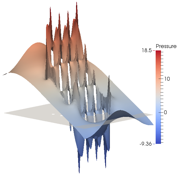
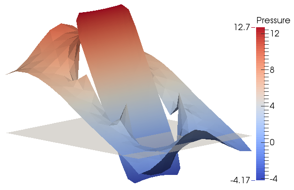
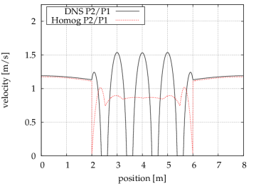
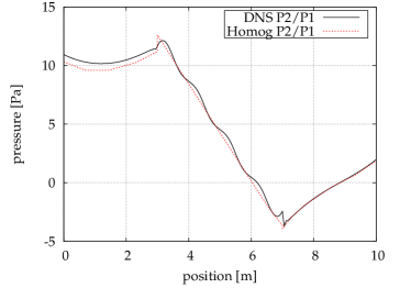
Figure 10: Flow over reinforced area: comparison of fully resolved solution (on the left) and homogenized solution (on the right) for a Newtonian fluid with $\mu=20$ and obstacle radius $\xi=0.125$.

4.2.2 Influence of the friction

This subsection is devoted to studying the effect of the friction, for the setup shown in Fig. 8 (left). The values of parameter $\beta$ are gradually increased from $0$ to $10$, as can be seen from results in Fig. 11. Velocity profiles in the v-section for different values of $\beta$ are shown on the left, while detailed view of velocity behavior near the interface between both the unperforated and the perforated region is shown on the right. The first row of pictures correspond to $\xi=0.125$, the second row to $\xi=0.25$ and the third to $\xi=0.35$.

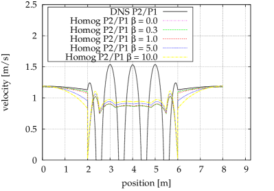
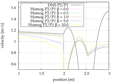
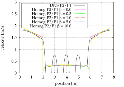
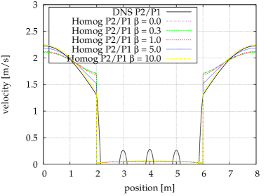
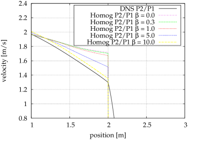
Figure 11: Flow over reinforced area: influence of the friction. The full velocity profiles are on the left, details near the interface between reinforced and unreinforced area are on the right. The top line figures show the case of $\xi=0.125$, the middle line of $\xi=0.25$ and the bottom line $\xi=0.35$.

It can be seen that in the case of $\xi=0.125$, with an increasing value of $\beta$, the agreement between homogenized and fully resolved solutions declines. The best agreement appears to be with $\beta=0$, which corresponds to no friction at all (full slip conditions). We believe that this phenomenon is caused by the fact that the effect of prescribed zero velocity on the obstacles (in the fully resolved case) does not propagate far enough, and so there is no “friction effect” at the interface in the homogenized case. Obviously $\beta=0$ would not be obtained with formula 21. This is caused by the particular $4\times 4$ setup used in our example, where the obstacles are too far from the interface $\Gamma$. In the limit case of infinitely many obstacles with radii tending to zero, significant influence of the friction could be expected. For a larger size of the obstacles, the situation is different, and with increasing perimeter of the obstacles, the influence of the friction becomes more important. For the case of $\xi=0.25$, the optimal value is $\beta\approx 3$, and for $\xi=0.35$, $\beta\approx 10$. Unfortunately, these values are not in agreement with the results presented [34]. In our opinion, there are several reasons for that. First, the geometry of the problem solved by the authors in [34] is not fully comparable with our problem, as they consider an infinite periodic domain, where the flow is realized only in the tangential direction to the interface $\Gamma$. In our case, the perforated domain has finite dimensions and we also allow the flow through the interface $\Gamma$.

For that reason and because of the possible material dependency in the case of non-linear fluids, we rather fit parameter $\beta$ according to agreement in the velocity profile near the interface. In particular, according to our numerical experiments (not shown), the optimal values of $\beta$ determined for a Newtonian fluid of viscosity $\mu$ performed well also for the regularized Bingham law (29) with the same plastic viscosity, $\mu_{0}=\mu$. In addition, for radii smaller than $\xi=0.125$, we systematically found that the optimal value of the coupling parameter $\beta$ equals $0$ also for non-Newtonian fluids, leading to the the full-slip interface conditions at $\Gamma$. This result is especially relevant in simulations of casting process in concrete structures, where $\xi\leq 0.125$ by construction requirements, see [47].

4.2.3 Bingham flow

This subsection illustrates the results for a Bingham fluid of plastic viscosity $\mu_{0}=20$, yield stress of $\tau_{0}=20$, and regularization parameter of $m=15$. The results are reported for RVEs with $\xi=0.125$ with $\beta=0$, and $\xi=0.25$ with $\beta=3$, for both horizontal and skew flows. Again, homogenized solution is validated against fully resolved solution from DNS.

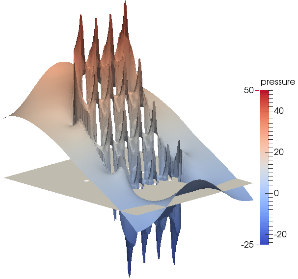
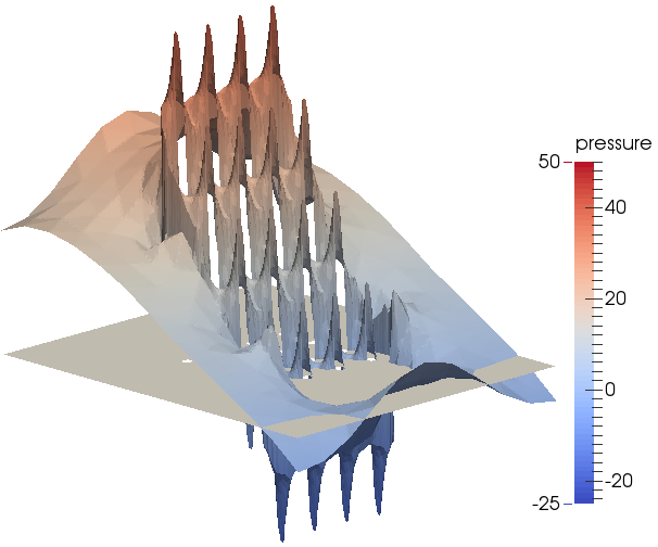
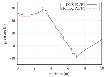
Figure 12: Flow over reinforced area: comparison of velocity and pressure profiles for Bingham fluid with $\mu_{0}=20$, $\tau_{0}=20$, and $m=15$, and RVE with $\xi=0.125$.

Fig. 12 shows the results for the horizontal setting and for $\xi=0.125$. The top row compares the pressure distributions of homogenized and fully resolved solutions in axonometric view. Note that here we show the reconstructed pressure with the added influence of the sub-scale pressure $p^{\mathrm{S}}$ obtained from the solution in the RVE according to the expansion (9a). The bottom row compares the velocity profiles over the section through the third column of obstacles (on the left), and the pressure profile over the horizontal section through the whole domain (on the right). These plots show only the averaged pressure and velocity. The results are in very good agreement, which can be seen in the bottom right picture with the pressure along the section through the whole domain. The macroscopic pressure gradient is captured extremely well. The oscillations close to the obstacles of course cannot be captured via homogenization approach. However, the average is in perfect agreement with the result obtained with DNS. The $\max$ norm error in average velocity inside the reinforced area is again less than 1%. The results for $\xi=0.25$, shown in Fig. 14, support the same conclusions.

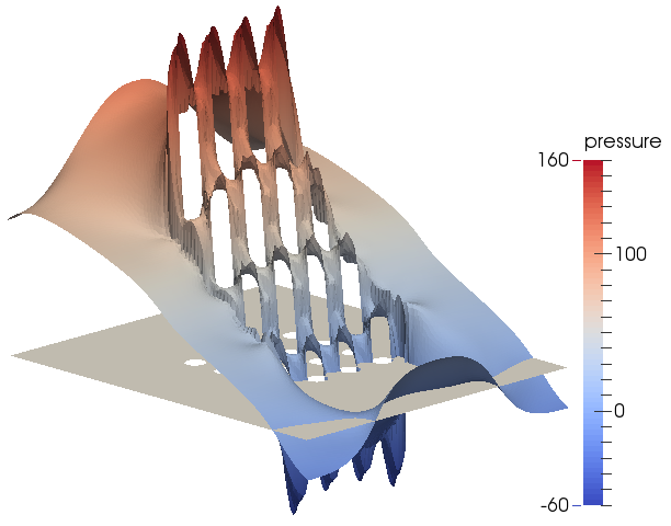
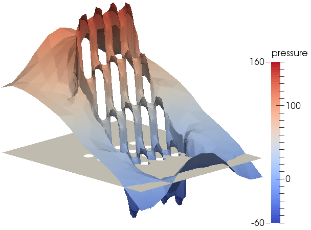
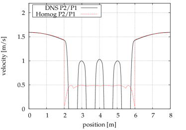
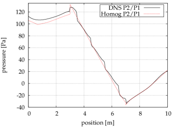
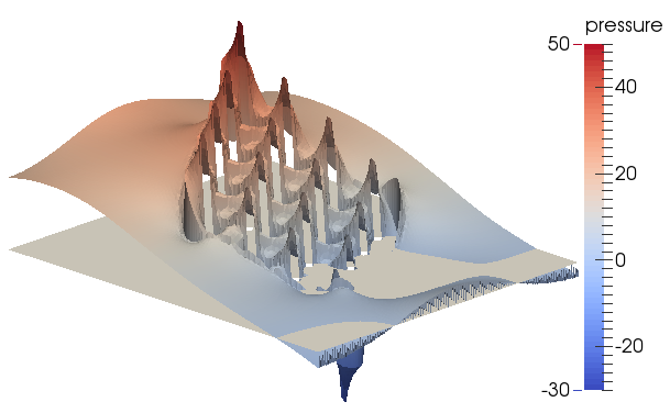
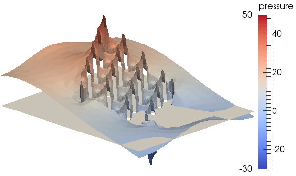
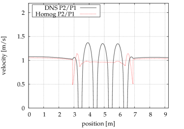
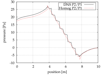
Figure 13: Flow over reinforced area: comparison of velocity and pressure profiles for Bingham fluid with $\mu_{0}=20$ and $\tau_{0}=20$, $m=15$.

Figure 14: Flow over reinforced area: comparison of velocity and pressure profiles for Bingham fluid in rotated setup with $\mu_{0}=20$, $\tau_{0}=20$, $m=15$, and RVE with $\xi=0.125$.

Figs. 14 and 15 show the results obtained for the rotated setup. Although the flow pattern is considerably more complex, the agreement of the results is also very good. The error in the average velocity through the reinforced domain is less than $5\%$ in the $\max$ norm.

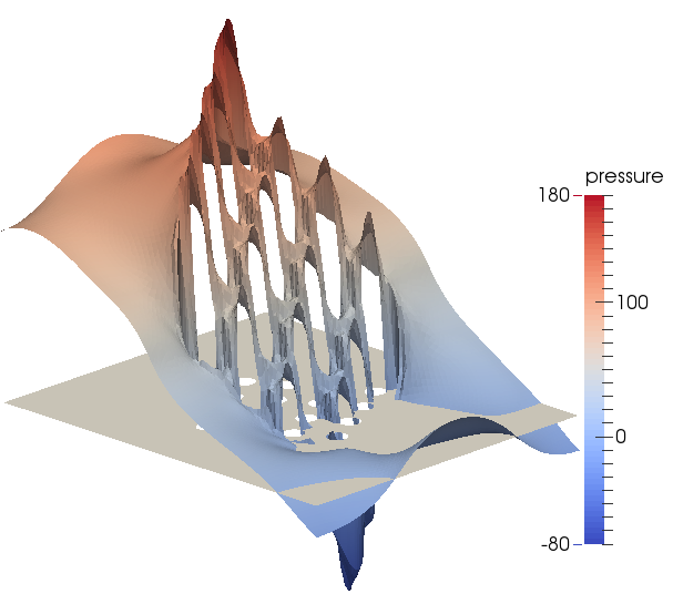
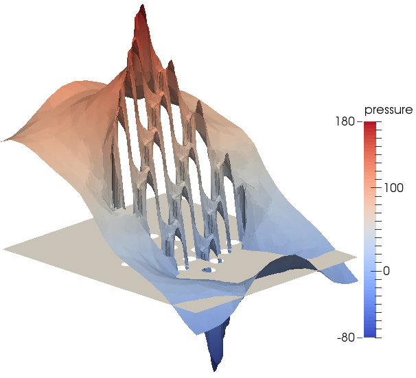
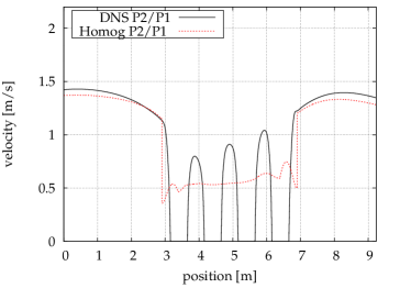
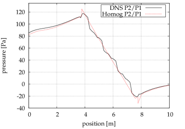
Figure 15: Flow over reinforced area: comparison of velocity and pressure profiles for Bingham fluid in rotated setup with $\mu_{0}=20$, $\tau_{0}=20$, $m=15$, and RVE with $\xi=0.25$.

5 Conclusions

In this paper, a computational homogenization approach to the flow of a non-Newtonian fluid through a perforated domain has been developed, with potential applications in simulations of concrete casting. We have presented a unified formulation of a coupled Stokes-Darcy system obtained by a variationally consistent homogenization of the Stokes flow in the porous sub-domain. Specifically, by introducing the decomposition of the pressure and corresponding test functions into macro and sub-scale parts in the perforated domain, the problem splits into a Darcy-type flow on the macro-scale, coupled to a nonlinear Stokes problem on the sub-scale, which is driven by the macroscopic pressure gradient. The consistent linearization of the ensuing problem has been presented, together with a numerical solution algorithm. The capabilities and potentials of the developed methodology have been illustrated by several examples comparing the homogenized solution with fully resolved simulations. On the basis of the obtained results, we conjecture that

1. in the reinforced domain, the homogenized non-linear Darcy law allows for a systematic and accurate incorporation of the effect of reinforcement into homogeneous models of (not only) fresh concrete,

2. in simulations of casting of self-compacting concrete, the full-slip conditions at the interface between the Stokes and Darcy domains deliver sufficiently accurate results with respect to the fully resolved model,

3. the parameters of the Beavers-Jones-Saffmann constitutive law determined by Jäger and Mikelić [32] for a free Newtonian fluid flow over a porous bed do not reflect the coupling between the Stokes and Darcy domains accurately, at least for the considered test cases. These findings seem to be consistent with a recent study of forced filtration of a Newtonian fluid into a porous medium by Carraro et al. [48], where different boundary conditions were derived by the refined asymptotic analysis and validated by direct numerical simulations. Additional studies are needed to clarify the interface conditions for non-Newtonian fluids.

References

- [1] H. Okamura, M. Ouchi, Self-compacting concrete, Journal of Advanced Concrete Technology 1 (1) (2003) 5–15.
- [2] P. L. Domone, Self-compacting concrete: An analysis of 11 years of case studies, Cement and Concrete Composites 28 (2) (2006) 197–208. doi:10.1016/j.cemconcomp.2005.10.003.
- [3] N. Roussel, M. R. Geiker, F. Dufour, L. N. Thrane, P. Szabo, Computational modeling of concrete flow: General overview, Cement and Concrete Research 37 (9) (2007) 1298–1307. doi:10.1016/j.cemconres.2007.06.007.
- [4] A. Gram, J. Silfwerbrand, Numerical simulation of fresh SCC flow: applications, Materials and Structures 44 (4). doi:10.1617/s11527-010-9666-9.
- [5] N. Roussel, A. Gram (Eds.), Simulation of Fresh Concrete Flow, Vol. 15 of RILEM State-of-the-Art Reports, Springer Netherlands, 2014.
- [6] V. Mechtcherine, A. Gram, K. Krenzer, J.-H. Schwabe, S. Shyshko, N. Roussel, Simulation of fresh concrete flow using Discrete Element Method (DEM): theory and applications, Materials and Structures 47 (4) (2013) 615–630. doi:10.1617/s11527-013-0084-7.
- [7] R. Deeb, S. Kulasegaram, B. L. Karihaloo, 3D modelling of the flow of self-compacting concrete with or without steel fibres. Part I: slump flow test, Computational Particle Mechanics 1 (4) (2014) 373–389. doi:10.1007/s40571-014-0002-y.
- [8] R. Deeb, S. Kulasegaram, B. L. Karihaloo, 3D modelling of the flow of self-compacting concrete with or without steel fibres. Part II: L-box test and the assessment of fibre reorientation during the flow, Computational Particle Mechanics 1 (4) (2014) 391–408. doi:10.1007/s40571-014-0003-x.
- [9] O. Švec, J. Skoček, H. Stang, M. R. Geiker, N. Roussel, Free surface flow of a suspension of rigid particles in a non-Newtonian fluid: A lattice Boltzmann approach, Journal of Non-Newtonian Fluid Mechanics 179–180 (2012) 32–42. doi:10.1016/j.jnnfm.2012.05.005.
- [10] C. Ferraris, F. De Larrard, N. Martys, Fresh concrete rheology: Recent developments, in: S. Mindess, J. Skalny (Eds.), Materials Science of Concrete VI, The American Ceramic Society, 2001, pp. 215–241.
- [11] P. F. G. Banfill, Rheology of fresh cement and concrete, Rheology Reviews 2006 (2006) 61–130.
- [12] F. Mahmoodzadeh, S. E. Chidiac, Rheological models for predicting plastic viscosity and yield stress of fresh concrete, Cement and Concrete Research 49 (2013) 1–9. doi:10.1016/j.cemconres.2013.03.004.
- [13] F. Dufour, G. Pijaudier-Cabot, Numerical modelling of concrete flow: homogeneous approach, International Journal for Numerical and Analytical Methods in Geomechanics 29 (4) (2005) 395–416. doi:10.1002/nag.419.
- [14] M. Cremonesi, L. Ferrara, A. Frangi, U. Perego, Simulation of the flow of fresh cement suspensions by a Lagrangian finite element approach, Journal of Non-Newtonian Fluid Mechanics 165 (23–24) (2010) 1555–1563. doi:10.1016/j.jnnfm.2010.08.003.
- [15] B. Patzák, Z. Bittnar, Modeling of fresh concrete flow, Computers & Structures 87 (15–16) (2009) 962–969. doi:10.1016/j.compstruc.2008.04.015.
- [16] F. Kolařík, B. Patzák, L. N. Thrane, Modeling of fiber orientation in viscous fluid flow with application to self-compacting concrete, Computers & Structures 154 (2015) 91–100. doi:10.1016/j.compstruc.2015.03.007.
- [17] K. Vasilic, B. Meng, H. C. Kühne, N. Roussel, Flow of fresh concrete through steel bars: A porous medium analogy, Cement and Concrete Research 41 (5) (2011) 496–503. doi:10.1016/j.cemconres.2011.01.013.
- [18] J. C. Michel, H. Moulinec, P. Suquet, Effective properties of composite materials with periodic microstructure: A computational approach, Computer Methods in Applied Mechanics and Engineering 172 (1–4) (1999) 109–143. doi:10.1016/S0045-7825(98)00227-8.
- [19] P. Kanouté, D. P. Boso, J. L. Chaboche, B. A. Schrefler, Multiscale methods for composites: A review, Archives of Computational Methods in Engineering 16 (1) (2009) 31–75. doi:10.1007/s11831-008-9028-8.
- [20] M. Geers, V. Kouznetsova, W. Brekelmans, Multi-scale computational homogenization: Trends and challenges, Journal of Computational and Applied Mathematics 234 (7) (2010) 2175–2182. doi:10.1016/j.cam.2009.08.077.
- [21] E. Sanchez-Palencia, Non-Homogeneous Media and Vibration Theory, Vol. 127 of Lecture Notes in Physics, Springer, Berlin, Heidelberg, 1980.
- [22] L. Tartar, Incompressible fluid flow in a porous medium – Convergence of the homogenization process, in: E. Sanchez-Palencia (Ed.), Non-Homogeneous Media and Vibration Theory, Vol. 127 of Lecture Notes in Physics, Springer, Berlin, Heidelberg, 1980, pp. 368–377.
- [23] G. Allaire, Homogenization of the Stokes flow in a connected porous medium, Asymptotic Analysis 2 (1989) 203–222.
- [24] A. Bourgeat, A. Mikelic, A note on homogenization of Bingham flow through a porous medium, Journal de Mathématiques Pures et Appliquées 72 (4) (1993) 405–414.
- [25] A. Bourgeat, A. Mikelić, Homogenization of a polymer flow through a porous medium, Nonlinear Analysis: Theory, Methods & Applications 26 (7) (1996) 1221–1253. doi:10.1016/0362-546X(94)00285-P.
- [26] U. Hornung (Ed.), Homogenization and Porous Media, Vol. 6 of Interdisciplinary Applied Mathematics, Springer, New York, NY, USA, 1997.
- [27] C. Sandström, F. Larsson, Variationally consistent homogenization of Stokes flow in porous media, International Journal for Multiscale Computational Engineering 11 (2013) 117–138. doi:10.1615/IntJMultCompEng.2012004069.
- [28] C. Sandström, F. Larsson, K. Runesson, H. Johansson, A two-scale finite element formulation of Stokes flow in porous media, Computer Methods in Applied Mechanics and Engineering 261–262 (2013) 96–104. doi:10.1016/j.cma.2013.03.025.
- [29] T. J. Hughes, G. R. Feijóo, L. Mazzei, J.-B. Quincy, The variational multiscale method - A paradigm for computational mechanics, Computer Methods in Applied Mechanics and Engineering 166 (1998) 3–24. doi:10.1016/S0045-7825(98)00079-6.
- [30] G. S. Beavers, D. D. Joseph, Boundary conditions at a naturally permeable wall, Journal of Fluid Mechanics 30 (1) (1967) 197–207. doi:10.1017/S0022112067001375.
- [31] P. G. Saffman, On the boundary condition at the surface of a porous medium, Studies in Applied Mathematics 50 (2) (1971) 93–101. doi:10.1002/sapm197150293.
- [32] W. Jäger, A. Mikelić, On the interface boundary condition of Beavers, Joseph, and Saffman, SIAM Journal on Applied Mathematics 60 (2000) 1111–1127. doi:10.1137/S003613999833678X.
- [33] W. Jäger, A. Mikelic, N. Neuss, Asymptotic analysis of the laminar viscous flow over a porous bed, SIAM Journal on Scientific Computing 22 (6) (2001) 2006–2028. doi:10.1137/S1064827599360339.
- [34] T. Carraro, C. Goll, A. Marciniak-Czochra, A. Mikelić, Pressure jump interface law for the Stokes–Darcy coupling: confirmation by direct numerical simulations, Journal of Fluid Mechanics 732 (2013) 510–536. doi:10.1017/jfm.2013.416.
- [35] M. Discacciati, E. Miglio, A. Quarteroni, Mathematical and numerical models for coupling surface and groundwater flows, Applied Numerical Mathematics 43 (1–2) (2002) 57–74. doi:10.1016/S0168-9274(02)00125-3.
- [36] J. Urquiza, D. N’Dri, A. Garon, M. Delfour, Coupling Stokes and darcy equations, Applied Numerical Mathematics 158 (2008) 525–538. doi:10.1016/j.apnum.2006.12.006.
- [37] T. Karper, K.-A. Mardal, R. Winther, Unified finite element discretizations of coupled Darcy–Stokes flow, Numerical Methods for Partial Differential Equations 25 (2009) 311–326. doi:10.1002/num.20349.
- [38] F. Kolařík, B. Patzák, J. Zeman, Modelling fresh concrete flow through reinforcing bars with computational homogenization, in: J. Kruis, Y. Tsompanakis, B. Topping (Eds.), Proceedings of the Fifteenth International Conference on Civil, Structural and Environmental Engineering Computing, Civil-Comp Press, Stirlingshire, UK, 2015, p. Paper 150. doi:10.4203/ccp.108.150.
- [39] F. Larsson, K. Runesson, F. Su, Variationally consistent computational homogenization of transient heat flow, International Journal for Numerical Methods in Engineering 81 (13) (2010) 1659–1686. doi:10.1002/nme.2747.
- [40] J. Sýkora, T. Krejčí, J. Kruis, M. Šejnoha, Computational homogenization of non-stationary transport processes in masonry structures, Journal of Computational and Applied Mathematics 236 (18) (2012) 4745–4755. doi:10.1016/j.cam.2012.02.031.
- [41] F. Brezzi, On the existence, uniqueness and approximation of saddle-point problems arising from Lagrangian multipliers, R.A.I.R.O. Anal. Numer. 8 (1974) 129–151.
- [42] I. Babuška, The finite element method with Lagrangian multipliers, Num. Math. 20 (1973) 179–192. doi:10.1007/BF01436561.
- [43] A. Quarteroni, R. Sacco, F. Saleri, Numerical mathematics, Springer-Verlag New York, Inc., 2006.
- [44] B. Patzák, Z. Bittnar, Design of object oriented finite element code, Advances in Engineering Software 32 (2001) 759–767. doi:10.1016/S0965-9978(01)00027-8.
- [45] B. Patzák, OOFEM - an object-oriented simulation tool for advanced modeling of materials and structures, Acta Polytechnica 52 (2012) 59–66.
- [46] T. C. Papanastasiou, Flows of materials with yield, Journal of Rheology 31 (1987) 385–404. doi:10.1122/1.549926.
- [47] Eurocode 2: Design of concrete structures - part 1-1: General rules and rules for buildings, Tech. Rep. ČSN EN 1992-1-1 (2006).
- [48] T. Carraro, C. Goll, A. Marciniak-Czochra, A. Mikelić, Effective interface conditions for the forced infiltration of a viscous fluid into a porous medium using homogenization, Computer Methods in Applied Mechanics and Engineering 292 (2015) 195–220. doi:10.1016/j.cma.2014.10.050.