MPP-2015-274
 
ATLAS Diboson Excess from Stueckelberg Mechanism

Abstract

We discuss the diboson excess seen by the ATLAS collaboration around 2 TeV in the LHC run I at $\sqrt{s}=8$ TeV. We explore the possibility that such an excess can arise from a $Z^{\prime}$ boson which acquires mass through a $U(1)_{X}$ Stueckelberg extension. The corresponding $Z^{\prime}$ gauge boson is leptophobic with a mass of around 2 TeV and has interactions with $SU(2)_{L}$ Yang-Mills fields and gauge fields of the hypercharge. The analysis predicts $Z^{\prime}$ decays into $WW$ and $ZZ$ as well as into $Z\gamma$. Further three-body as well as four-body decays of the $Z^{\prime}$ such as $WWZ$, $WW\gamma$, $WWZZ$ etc are predicted. In the analysis we use the helicity formalism which allows us to exhibit the helicity structure of the $Z^{\prime}$ decay processes in an transparent manner. In particular, we are able to show the set of vanishing helicity amplitudes in the decay of the massive $Z^{\prime}$ into two vector bosons due to angular momentum conservation with a special choice of the reference momenta. The residual set of non-vanishing helicity amplitudes are identified. The parameter space of the model compatible with the diboson excess seen by the ATLAS experiment at $\sqrt{s}=8$ TeV is exhibited. Estimate of the diboson excess expected at $\sqrt{s}=13$ TeV with 20 fb^-1 of integrated luminosity at LHC run II is also given. It is shown that the $WW$, $ZZ$ and $Z\gamma$ modes are predicted to be in the approximate ratio $1:\cos^{2}\theta_{W}(1+\alpha\tan^{2}\theta_{W})^{2}/2:(1-\alpha)^{2}\sin^{2}\theta_{W}/2$ where $\alpha$ is the strength of the coupling of $Z^{\prime}$ with the hypercharge gauge field relative to the coupling with the Yang-Mills gauge fields. Thus observation of the $Z\gamma$ mode as well as three-body and four-body decay modes of the $Z^{\prime}$ will provide a definite test of the model and of a possible new source of interaction beyond the standard model.

1 Introduction

The ATLAS collaboration at CERN [1] has seen a diboson excess around $2$ TeV in the $WZ$, $WW$, and $ZZ$ channels with local significance of 3.4$\sigma$, 2.6$\sigma$, and 2.9$\sigma$ in that order. In this work we discuss a model where the source of the diboson excess is a $Z^{\prime}$ boson which gains mass through the Stueckelberg mechanism [2, 3, 4, 5, 6, 7] and has interactions with $SU(2)_{L}$ Yang-Mills gauge bosons. Our model differs in significant ways from a variety of other models that have been proposed to explain the excess. These include models with strong dynamics [8], $W^{\prime}$ models [9], models based on strings [10], composite spin zero boson models [11], and many others [12].

2 $Z^{\prime}$ to Diboson decays

We consider a $U(1)_{X}$ extension of the standard model with $C_{\mu}(x)$ as the gauge boson and we propose the following effective interaction

$${\cal L}={{1\over\Lambda^{2}}}\Big{[}\Big{(}{1\over M}\partial_{\mu}\sigma+C_{\mu}\Big{)}\partial_{\nu}\,\big{(}F_{a}^{\mu\lambda}{F^{~{}\nu}_{a~{}\lambda}}+\alpha B^{\mu\lambda}B^{\nu}_{\lambda}\big{)}+\big{(}\mu\leftrightarrow\nu\big{)}\Big{]}\,,$$ (1)

where $F$ and $B$ are the $SU(2)_{L}$ and $U(1)_{Y}$ field strengths, $a$ is the $SU(2)_{L}$ index, $\alpha$ is the strength of the coupling of $C_{\mu}$ with the hypercharge gauge field relative to the coupling with the Yang-Mills gauge fields and is a free parameter, and the new physics scale $\Lambda$ will be determined by experiment. In Eq. 1 we are using the Stueckelberg mechanism to make the Lagrangian gauge invariant. This occurs due to the following gauge transformations of $C_{\mu}$ and $\sigma$: $C_{\mu}\to C_{\mu}-\partial_{\mu}\lambda\,,\ \sigma\to M\lambda$. Thus the interactions is $U(1)_{X}$ and $SU(2)_{L}$ gauge invariant. For more details of Stueckelberg mechanism and the Stueckelberg $U(1)$ extension of standard model or minimal supersymmetric standard model, see [2].

In the unitary gauge we define $Z^{\prime}_{\mu}=({1\over M}\partial_{\mu}\sigma+C_{\mu})$. These interactions will describe the possible decays of the $Z^{\prime}$ into two-body, three-body and four-body states. After expansion, the three-point interactions read

$$\mathcal{L}_{{\rm 3pt}}=\frac{2}{\Lambda^{2}}\,Z_{\mu}^{\prime}\big{(}\partial^{\nu}A^{\mu}_{a}\,\partial^{2}A_{a\nu}-\partial^{\mu}A^{\nu}_{a}\,\partial^{2}A_{a\nu}+\alpha\,\partial^{\nu}B^{\mu}\,\partial^{2}B_{\nu}-\alpha\,\partial^{\mu}B^{\nu}\,\partial^{2}B_{\nu}\big{)}\,.$$ (2)

Further after spontaneous breaking of the electroweak symmetry we will have a Lagrangian describing the interactions of the $Z^{\prime}$ with $W,Z$ and $\gamma$. For the two-body decays the possible modes are $W^{+}W^{-}$, $ZZ$, $Z\gamma$. In addition, Eq. 1 also provides three- and four-body decays such as $W^{+}W^{-}Z$, $W^{+}W^{-}\gamma$ and $W^{+}W^{-}ZZ$ etc. For the two-body decay, Eq. 2 further reduces to

$$\mathcal{L}_{{\rm 3pt}} =\frac{{2}m_{W}^{2}}{\Lambda^{2}}Z^{\prime}_{\mu}(\partial^{\nu}W^{-\mu}W_{\nu}^{+}+\partial^{\nu}W^{+\mu}W_{\nu}^{-})$$

$$\,+\frac{{2}m_{Z}^{2}}{\Lambda^{2}}Z^{\prime}_{\mu}\left[\cos^{2}\theta_{W}\partial^{\nu}Z^{\mu}Z_{\nu}+\sin\theta_{W}\cos\theta_{W}(\partial^{\nu}A^{\mu}Z_{\nu}-\partial^{\mu}A^{\nu}Z_{\nu})\right]$$

$$\,+\frac{{2}m_{Z}^{2}}{\Lambda^{2}}\,\alpha\,Z^{\prime}_{\mu}\left[\sin^{2}\theta_{W}\partial^{\nu}Z^{\mu}Z_{\nu}-\sin\theta_{W}\cos\theta_{W}(\partial^{\nu}A^{\mu}Z_{\nu}-\partial^{\mu}A^{\nu}Z_{\nu})\right]\,,$$ (3)

where $\sin\theta_{W}=g/\sqrt{g^{2}+g^{\prime 2}},\cos\theta_{W}=g^{\prime}/\sqrt{g^{2}+g^{\prime 2}}$. First we notice $Z^{\prime}$ to diphoton channel automatically vanishes consistent with the Landau-Yang theorem [16, 17, 18, 19, 20]. As seen from Eq. 3 the non-vanishing two-body decays consist of the final states $W^{+}W^{-}$, $ZZ$, $Z\gamma$. For the case $\alpha=1$ the $Z^{\prime}\to Z\gamma$ mode vanishes. In the analysis of these final states we will use the helicity formalism. In this formalism the three-point amplitudes for these processes read

$$\mathscr{A} \big{[}Z^{\prime}(\xi^{\prime},k^{\prime})\to W^{+}(\xi_{1}^{+},k_{1})W^{-}(\xi_{2}^{-},k_{2})\big{]}=\frac{{2}m_{W}^{2}}{\Lambda^{2}}\big{[}(\xi^{\prime*}\cdot\xi_{2}^{-})(\xi_{1}^{+}\cdot k_{2})+(\xi^{\prime*}\cdot\xi_{1}^{+})(\xi_{2}^{-}\cdot k_{1})\big{]}\,,$$ (4)

$$\mathscr{A} \big{[}Z^{\prime}(\xi^{\prime},k^{\prime})\to Z(\xi_{1},k_{1})Z(\xi_{2},k_{2})\big{]}=\frac{{2}m_{Z}^{2}}{\Lambda^{2}}(\cos^{2}\theta_{W}+\alpha\sin^{2}\theta_{W})\times$$

$$\qquad\qquad\qquad\qquad\qquad\qquad\qquad\qquad\qquad\qquad\qquad\big{[}(\xi^{\prime*}\cdot\xi_{2})(\xi_{1}\cdot k_{2})+(\xi^{\prime*}\cdot\xi_{1})(\xi_{2}\cdot k_{1})\big{]}\,,$$ (5)

$$\mathscr{A} \big{[}Z^{\prime}(\xi^{\prime},k^{\prime})\to Z(\xi,k)\gamma(\epsilon,k_{0})\big{]}=\frac{2m_{Z}^{2}}{\Lambda^{2}}(1-\alpha)\sin\theta_{W}\cos\theta_{W}\big{[}(\xi^{\prime*}\cdot\epsilon)(\xi\cdot k_{0})-(\xi^{\prime*}\cdot k_{0})(\xi\cdot\epsilon)\big{]}\,,$$ (6)

where $\xi^{\prime},\xi_{\pm},\xi,\epsilon$ denote the polarization vector of $Z^{\prime},W^{\pm},Z,\gamma$. To see the helicity structure of the above amplitudes more explicitly, we now apply the spinor helicity formalism. A massless spin one gauge boson has two degrees of freedom, corresponding to up and down helicities. They are expressed by the polarization vectors $\text{$\epsilon$}_{\mu}^{+}$ and $\text{$\epsilon$}_{\mu}^{-}$ and can be written as [13]

$$\text{$\epsilon$}_{\mu}^{+}(k,r)=\frac{r_{\dot{a}}^{*}\bar{\sigma}_{\mu}^{\dot{a}a}k_{a}}{\sqrt{2}r_{\dot{a}}^{*}k^{*\dot{a}}}\,,\qquad\text{$\epsilon$}_{\mu}^{-}(k,r)=\frac{k_{\dot{a}}^{*}\bar{\sigma}_{\mu}^{\dot{a}a}r_{a}}{\sqrt{2}k^{a}r_{a}}\,,$$ (7)

where $k$ is the momentum of the particle and $r$ is the reference momentum which can be chosen to be any light-like momentum except $k$. Here the momenta with spinor indices are $2$-component commutative spinors, and they are defined as $p_{\mu}\sigma^{\mu}_{a\dot{a}}=-p_{a}p^{*}_{\dot{a}}$. It’s easy to show $\epsilon_{+}^{\mu}(k,r)-\epsilon_{+}^{\mu}(k,\tilde{r})\sim k^{\mu}$ where $\tilde{r}$ is some other free chosen reference momentum. Since the whole amplitude is invariant under the gauge transformation $\epsilon^{\mu}\to\epsilon^{\mu}+\lambda k^{\mu}$, choosing different reference momentum for a massless gauge boson does not change the result.

A massive spin one gauge boson which is expressed by its polarization vector $\xi_{\mu}$, contains three degrees of freedom associated to the eigenstates of $J_{z}$, where the transversality condition $\xi_{\mu}k^{\mu}=0$ eliminates one degree of freedom of the four-vector. The choice of the quantization axis $\vec{z}$ can be handled in an elegant way by decomposing the momentum $k^{\mu}$ into two arbitrary light-like reference momenta $p$ and $q$:

$$k^{\mu}=p^{\mu}+q^{\mu}\,,\qquad k^{2}=-m^{2}=2pq\,,\qquad p^{2}=q^{2}=0\,.$$ (8)

Once the reference momenta $p$ and $q$ are chosen, the spin quantization axis of the polarization vector $\xi_{\mu}$ is set to be collinear to the direction of $\vec{q}$ in the rest frame. The 3 spin wave functions depend on $p$ and $q$, while this dependence would drop out in the squared amplitudes summing over all spin directions. The massive spin one wave functions $\xi_{\mu}$ are given by the following polarization vectors (up to a phase factor) [14, 15]

$$\text{$\xi$}^{\mu}(k,J_{z}=+1) =\frac{1}{\sqrt{2}m}p_{\dot{a}}^{*}\bar{\sigma}^{\mu\dot{a}a}q_{a}\,,$$ (9)

$$\text{$\xi$}^{\mu}(k,J_{z}=\ 0\ ) =\frac{1}{2m}\bar{\sigma}^{\mu\dot{a}a}(p_{\dot{a}}^{*}p_{a}-q_{\dot{a}}^{*}q_{a})\,,$$ (10)

$$\text{$\xi$}^{\mu}(k,J_{z}=-1) =-\frac{1}{\sqrt{2}m}q_{\dot{a}}^{*}\bar{\sigma}^{\mu\dot{a}a}p_{a}\,.$$ (11)

With different choices of reference momenta $(p,q)$, one will get different helicity amplitudes. While the $(p,q)$-dependence would drop off when one adds up all the squared helicity amplitudes. Since we have the freedom to choose reference momenta for the interacting spin one gauge bosons, with a clever choice one can not only simplify the computation dramatically but also exhibit the helicity structure in a transparent manner.

For the process $Z^{\prime}(k^{\prime})\to Z(k)\gamma(k_{0})$, since the spin quantization axis of a massless photon is collinear to its moving direction, we choose the following reference momenta

$$\gamma\ \qquad\epsilon(k_{0}): \qquad r\,,$$ (12)

$$Z\ \ \qquad\xi(k): \qquad k=r+ak_{0}\,,$$ (13)

$$Z^{\prime}\qquad\xi^{\prime}(k^{\prime}): \qquad k^{\prime}=r+(a+1)k_{0}\,,$$ (14)

where $r^{2}=0$ and $a=m_{Z}^{2}/(M_{Z^{\prime}}^{2}-m_{Z}^{2})$. For this clever choice, the spin quantization axes of both $Z^{\prime}$ and $Z$ are aligned to the photon moving direction, i.e., the direction of $\vec{k}_{0}$.

For $Z^{\prime}$ decay into two massive gauge bosons with a common mass $m_{i}$, where $m_{i}=m_{W}$ for Eq. (4) and $m_{i}=m_{Z}$ for Eq. (5), we choose the following reference momenta

$$Z_{1}/W^{+}\qquad\xi_{1}(k_{1}): \qquad k_{1}=cp+q\,,$$ (15)

$$Z_{2}/W^{-}\qquad\xi_{2}(k_{2}): \qquad k_{2}=p+cq\,,$$ (16)

$$Z^{\prime}\quad\ \ \qquad\xi^{{}^{\prime}}(k^{\prime}): \qquad k^{\prime}=(1+c)p+(1+c)q\,,$$ (17)

with $m_{i}^{2}=k_{1}^{2}=k_{2}^{2}=2cp\cdot q$, $M_{Z^{\prime}}^{2}=k^{\prime 2}=2(1+c)^{2}p\cdot q$, and thus

$$c_{i}=\frac{1}{2}(b_{i}-2)\pm\frac{1}{2}\sqrt{b_{i}^{2}-4b_{i}}\,,$$ (18)

where $b_{i}=M_{Z^{\prime}}^{2}/m_{i}^{2}$. Under this choice of reference momenta, the spin quantization axes of all these three massive gauge bosons are aligned to the same direction, i.e., the direction of $\vec{q}$.

In sum, for the two cases discussed above the spin quantization axes of the decaying massive gauge boson $Z^{\prime}$ as well as the two gauge bosons in the final state, are aligned to the same direction. Thus for the process $Z^{\prime}\to Z\gamma$, it is not difficult to show the vanishing of the following helicity amplitudes

$$\mathscr{A}\big{[}Z^{\prime};Z(+),\gamma(+)\big{]}=\mathscr{A}\big{[}Z^{\prime};Z(-),\gamma(-)\big{]}=0\,,$$ (19)

$$\mathscr{A}\big{[}Z^{\prime}(\pm);Z(+),\gamma(-)\big{]}=\mathscr{A}\big{[}Z^{\prime}(\pm);Z(-),\gamma(+)\big{]}=0\,,$$ (20)

as a result of angular momentum conservation, c.f., the left panel of Fig. 1. While the non-vanishing helicity amplitudes are

$$\mathscr{A}_{1} \equiv\mathscr{A}\big{[}Z^{\prime}(+);Z(0),\gamma(+)\big{]}=\mathscr{A}\big{[}Z^{\prime}(-);Z(0),\gamma(-)\big{]}=\frac{\sin\theta_{W}\cos\theta_{W}}{{\Lambda^{2}}}\beta m_{Z}(M_{Z^{\prime}}^{2}-m_{Z}^{2})\,,$$ (21)

$$\mathscr{A}_{2} \equiv\mathscr{A}\big{[}Z^{\prime}(0);Z(+),\gamma(-)\big{]}=\mathscr{A}\big{[}Z^{\prime}(0);Z(-),\gamma(+)\big{]}=\frac{\sin\theta_{W}\cos\theta_{W}}{{\Lambda^{2}M_{Z^{\prime}}^{2}}}\beta m_{Z}^{2}(M_{Z^{\prime}}^{2}-m_{Z}^{2})\,,$$ (22)

where $\beta\equiv 1-\alpha$. Thus the total squared-amplitude read

$$Z^{\prime}\to Z\gamma:\quad\sum|\mathscr{A}|^{2}=2|\mathscr{A}_{1}|^{2}+2|\mathscr{A}_{2}|^{2}=\frac{{2}\sin^{2}\theta_{W}\cos^{2}\theta_{W}\beta^{2}}{\Lambda^{4}}\frac{m_{Z}^{2}}{M_{Z^{\prime}}^{2}}(M_{Z^{\prime}}^{2}+m_{Z}^{2})(M_{Z^{\prime}}^{2}-m_{Z}^{2})^{2}\,.$$ (23)

The factor 2 in $2|\mathscr{A}_{1}|^{2}$ and $2|\mathscr{A}_{2}|^{2}$ arise because for each there are two helicity configurations, c.f., Eqs. 21 and 22, that are non-vanishing.

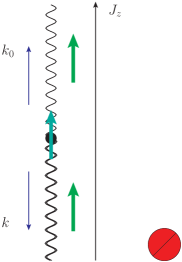
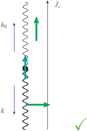
Figure 1: [Color online] The black dots in the center denote the decaying $Z^{\prime}$. In the center of mass frame, after decay the photon and $Z$ in the final state are moving to the opposite directions. The single wavy lines present the photon and the double wavy lines present the $Z$. The spin of the photon is along (or opposite to) its moving direction. We choose the reference momenta of the massive $Z$ as well as the $Z^{\prime}$ in such a way that their spin quantization axes ($\vec{J_{z}}$) are aligned to the photon moving direction. The emerald arrows present the spin of the $Z^{\prime}$, and the green arrows show the spin of the photon and $Z$. The left panel presents the vanishing helicity amplitude $\mathscr{A}\big{[}Z^{\prime}(+);Z(+),\gamma(+)\big{]}=0$ and this process is not allowed as indicated by the red forbidden sign. The right panel shows the non-vanishing helicity amplitude $\mathscr{A}\big{[}Z^{\prime}(+);Z(0),\gamma(+)\big{]}$ and this process is allowed as indicated by the green check sign.

Next we discuss the $Z^{\prime}$ decay into two massive gauge bosons. An analysis similar to the above gives

$$\mathscr{A}\big{[}Z^{\prime}(+);+,+\big{]}=\mathscr{A}\big{[}Z^{\prime}(+);-,-\big{]}=\mathscr{A}\big{[}Z^{\prime}(+);0,0\big{]}=\mathscr{A}\big{[}Z^{\prime}(+);+,-\big{]}=0\,,$$ (24)

$$\mathscr{A}\big{[}Z^{\prime}(-);-,-\big{]}=\mathscr{A}\big{[}Z^{\prime}(-);+,+\big{]}=\mathscr{A}\big{[}Z^{\prime}(-);0,0\big{]}=\mathscr{A}\big{[}Z^{\prime}(-);+,-\big{]}=0\,,$$ (25)

$$\mathscr{A}\big{[}Z^{\prime}(0);+,+\big{]}=\mathscr{A}\big{[}Z^{\prime}(0);-,-\big{]}=\mathscr{A}\big{[}Z^{\prime}(0);+,0\big{]}=\mathscr{A}\big{[}Z^{\prime}(0);-,0\big{]}=0\,,$$ (26)

$$\mathscr{A}\big{[}Z^{\prime}(0);+,-\big{]}=\mathscr{A}\big{[}Z^{\prime}(0);-,+\big{]}=\mathscr{A}\big{[}Z^{\prime}(0);0,0\big{]}=0\,,$$ (27)

where the first three lines are due to angular momentum conservation, c.f., the left panel of Fig. 2 and the last line is due to the special choice of the reference momenta Eqs. 15, 16 and 17. The residual set of non-vanishing helicity amplitudes are

$$\mathscr{A}_{3}\equiv\mathscr{A}\big{[}Z^{\prime}(+);+,0\big{]}=\mathscr{A}\big{[}Z^{\prime}(+);0,+\big{]}=\mathscr{A}\big{[}Z^{\prime}(-);-,0\big{]}=\mathscr{A}\big{[}Z^{\prime}(-);0,-\big{]}\,.$$ (28)

Explicitly they are given by

$$\mathscr{A}_{3W} \equiv\mathscr{A}(Z^{\prime}\to W^{+}W^{-})=\frac{m_{W}^{4}}{{\Lambda^{2}}M_{Z^{\prime}}}\frac{(c_{W}+1)^{2}(c_{W}-1)}{c_{W}^{3/2}}\,,$$ (29)

$$\mathscr{A}_{3Z} \equiv\mathscr{A}(Z^{\prime}\to ZZ)=\frac{(\cos^{2}\theta_{W}+\alpha\sin^{2}\theta_{W})m_{Z}^{4}}{\Lambda^{2}M_{Z^{\prime}}}\frac{(c_{Z}+1)^{2}(c_{Z}-1)}{c_{Z}^{3/2}}\,,$$ (30)

where the coefficients $c_{i}$ are given in Eq. 18, and $m_{i}=m_{W}$ for Eq. (29) and $m_{i}=m_{Z}$ for Eq. (30). The total squared-amplitudes read

$$Z^{\prime}\to W^{+}W^{-}:\qquad \sum|\mathscr{A}|^{2}=4|\mathscr{A}_{3W}|^{2}=\frac{{4}}{\Lambda^{4}}M_{Z^{\prime}}^{2}m_{W}^{2}(M_{Z^{\prime}}^{2}-4m_{W}^{2})\,,$$ (31)

$$Z^{\prime}\to ZZ:\qquad \sum|\mathscr{A}|^{2}=2|\mathscr{A}_{3Z}|^{2}=\frac{2(\cos^{2}\theta_{W}+\alpha\sin^{2}\theta_{W})^{2}}{{\Lambda^{4}}}M_{Z^{\prime}}^{2}m_{Z}^{2}(M_{Z^{\prime}}^{2}-4m_{Z}^{2})\,.$$ (32)

Here the factor 4 for $W^{+}W^{-}$ channel is due to the fact that there are in total 4 non-vanishing helicity amplitudes in this channel, c.f., Eq. 28. The factor 2 for $ZZ$ channel is due to the fact that there are only 2 non-vanishing helicity amplitudes since the two final state particles are identical, e.g., $\mathscr{A}\big{[}Z^{\prime}(+);+,0\big{]}$ and $\mathscr{A}\big{[}Z^{\prime}(+);0,+\big{]}$ give the same amplitude for $Z^{\prime}\to ZZ$ channel.

In summary, by using the helicity formalism, we can see clearly which helicity modes are forbidden as a result of angular momentum conservation, c.f., Eqs. 19, 20, 24, 25 and 26 and also Figs. 1 and 2. In addition, there are multiple helicity amplitudes which vanish due to the clever choice of the reference momenta, c.f., Eq. 27.

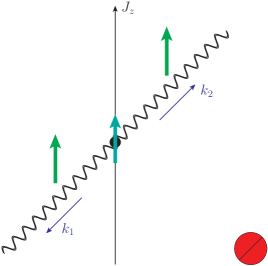
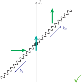
Figure 2: [Color online] In the center of mass frame, after the decay the two massive gauge bosons in the final state are moving to the opposite directions. The black dots in the center again denote the decaying $Z^{\prime}$. We have chosen the reference momenta in such a way that the spin quantization axes of these three gauge bosons are aligned to the same direction, i.e., $\vec{J_{z}}$. In general, for a massive gauge boson, the direction of $\vec{J_{z}}$ is different with its moving direction because one can always boost it to other reference frames. The emerald arrows present the spin of the $Z^{\prime}$, and the green arrows show the spin of the two final state gauge bosons. The left panel presents the vanishing helicity amplitude $\mathscr{A}\big{[}Z^{\prime}(+);+,+\big{]}$, and the right panel shows the non-vanishing helicity amplitude $\mathscr{A}\big{[}Z^{\prime}(+);0,+\big{]}$.

Using the above the partial decay widths for the processes $WW$, $ZZ$, $Z\gamma$ are given by

$$\Gamma(Z^{\prime}\to W^{+}W^{-}) =\frac{1}{{4}\pi}\frac{m_{W}^{2}(M_{Z^{\prime}}^{2}-4m_{W}^{2})^{3/2}}{\Lambda^{4}}\,,$$ (33)

$$\Gamma(Z^{\prime}\to ZZ) =\frac{(\cos^{2}\theta_{W}+\alpha\sin^{2}\theta_{W})^{2}}{8\pi}\frac{m_{Z}^{2}(M_{Z^{\prime}}^{2}-4m_{Z}^{2})^{3/2}}{\Lambda^{4}}\,,$$ (34)

$$\Gamma(Z^{\prime}\to Z\gamma) =\frac{(1-\alpha)^{2}\sin^{2}\theta_{W}\cos^{2}\theta_{W}}{{8}\pi}\frac{m_{Z}^{2}(M_{Z^{\prime}}^{2}+m_{Z}^{2})(M_{Z^{\prime}}^{2}-m_{Z}^{2})^{3}}{\Lambda^{4}M_{Z^{\prime}}^{5}}\,.$$ (35)

In the limit $M^{2}_{Z^{\prime}}\gg m^{2}_{W},m^{2}_{Z}$ which holds to better than 1% accuracy one has the following ratio among the three decay modes

$$\Gamma(W^{+}W^{-}):\Gamma(ZZ):\Gamma(Z\gamma)\simeq 2:\cos^{2}\theta_{W}(1+\alpha\tan^{2}\theta_{W})^{2}:(1-\alpha)^{2}\sin^{2}\theta_{W}\,.$$ (36)

For the case $\alpha=0$, the above ratio reduces to

$$\Gamma(W^{+}W^{-}):\Gamma(ZZ):\Gamma(Z\gamma)\simeq 2:\cos^{2}\theta_{W}:\sin^{2}\theta_{W}\,,$$ (37)

and for the case $\alpha=1$, the above ratio gives

$$\Gamma(W^{+}W^{-}):\Gamma(ZZ):\Gamma(Z\gamma)\simeq 2:\cos^{-2}\theta_{W}:0\,.$$ (38)

Thus we see that both the $ZZ$ and the $Z\gamma$ modes are highly model dependent and they could be vanishing or non-vanishing depending on the value of $\alpha$ (which can be either positive or negative); more LHC data are needed to fully discriminate the three diboson channels and to fix the $\alpha$ parameter.

3 Phenomenology

Regarding the coupling of the $Z^{\prime}$ to the standard model fermions, we will assume a leptophobic $Z^{\prime}$ with the following direct interaction to quarks

$${\cal L}_{\text{int}}=g_{X}Z^{\prime}_{\mu}\bar{q}\gamma^{\mu}q\,.$$ (39)

The decay width to quarks due to the direct couplings is given by

$$\Gamma_{\text{direct}}=N_{c}N_{f}g_{X}^{2}{M_{Z^{\prime}}\over 12\pi}\,,$$ (40)

where $N_{c}=3$ is the QCD color factor, and $N_{f}$ is the number of quark flavors that the $Z^{\prime}$ can decay into which is the number of kinematically allowed flavors. Without going into details we assume that our $U(1)_{X}$ with a gauged baryon number is anomaly free. Such a $U(1)_{X}$ can arise in a variety of settings such as from gut models [21], or anomaly-free family-dependent $U(1)$’s [22], with extra heavy chiral particles to cancel the anomaly [23, 24, 25, 26]. We further assume that the heavy chiral states are not accessible at the current LHC energy and thus do not enter in $Z^{\prime}$ decay.

We discuss now the production cross section of the $Z^{\prime}$ at LHC at $\sqrt{s}=8$ TeV and estimate the size of the diboson excess. The parton level cross section for the process $q\bar{q}\to Z^{\prime}\to W^{+}W^{-}$ using Breit-Wigner form for the $Z^{\prime}$ intermediate state is given by

$$\hat{\sigma}(q\bar{q}\to Z^{\prime}\to W^{+}W^{-})={1\over 12\pi\Lambda_{\rm eff}^{4}}\sqrt{1-4m_{W}^{2}/\hat{s}}{\hat{s}M_{Z^{\prime}}^{2}(\hat{s}-4M_{Z^{\prime}}^{2}x_{W}^{2})x_{W}^{2}\over(\hat{s}-M_{Z^{\prime}}^{2})^{2}+\hat{s}^{2}\Gamma_{Z^{\prime}}^{2}M_{Z^{\prime}}^{-2}}\,,$$ (41)

where $\Lambda^{2}_{\text{eff}}=\Lambda^{2}/g_{X}$, $x_{W}\equiv m_{W}/m_{Z^{\prime}}$. The $q\bar{q}\to Z^{\prime}\to ZZ$ cross section can be obtained easily if one replaces $m_{W}$ by $m_{Z}$ and inserts the overall factor $(\cos^{2}\theta_{W}+\alpha\sin^{2}\theta_{W})^{2}/2$ to the above $W^{+}W^{-}$ cross section. The hadron cross section at the LHC ($\sqrt{s}=8$ TeV) is computed via the convolution

$$\sigma(pp\to Z^{\prime}\to W^{+}W^{-})=K\int d\tau\,\hat{\sigma}(\hat{s}=s\tau)\,{d{\cal L}\over d\tau}(\tau)$$ (42)

where we use $K\simeq 1.3$ [27] [28] to approximate the next to leading correction and ${d{\cal L}/d\tau}$ is the parton luminosity given by ${d{\cal L}/d\tau}(\tau)=2\int_{\tau}^{1}(dx/x)\left[u(x)\bar{u}\left({\tau/x}\right)+d(x)\bar{d}\left({\tau/x}\right)\right]$.

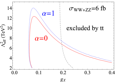
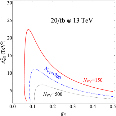
Figure 3: Left panel: Analysis at $\sqrt{s}=8$ TeV using events over the energy range $1.8$ TeV $<\sqrt{\hat{s}}<2.2$ TeV computed for both $\alpha=0$ and $\alpha=1$ cases: The red solid (blue dashed) curve predicts $\sigma_{\rm WW+ZZ}=6$ fb for the $\alpha=0$ ($\alpha=1$) case, where the Breit-Wigner effects of the $Z^{\prime}$ resonance have been taken into account. The parameter region on the right hand side of the gray dot-dashed curve is excluded by the $t\bar{t}$ resonance search at the LHC. Right panel: Expected number of events in the energy range $1.8$ TeV $<m_{VV}<2.2$ TeV with an integrated luminosity 20 fb^-1 at LHC run II at $\sqrt{s}=13$ TeV. Here $VV$ includes both $WW$ and $ZZ$ events. We take $\alpha=0$ here, and assume the same event selection efficiency with event topology requirements as given in the ATLAS analysis [1], which is $\sim$80%.

The most stringent LHC constraints for the leptophobic $Z^{\prime}$ come from the $t\bar{t}$ resonance search [29] [30], and the dijet channel [31] [32]. The 95% CL upper limit on dijet cross section for a 2 TeV $Z^{\prime}$ is $\sigma(Z^{\prime})\times\text{BR}(Z^{\prime}\to q\bar{q})<100$ fb [31]. For $t\bar{t}$ resonance search, the 95% CL upper limit for a 2 TeV $Z^{\prime}$ is $\sigma(Z^{\prime})\times\text{BR}(Z^{\prime}\to t\bar{t})<11$ (18) fb when $\Gamma_{Z^{\prime}}=20$ (200) GeV [29]. We use 11 fb as the limit in the $t\bar{t}$ channel for $\Gamma_{Z^{\prime}}\leq 20$ GeV, 18 fb for $\Gamma_{Z^{\prime}}\geq 200$ GeV, and linearly interpolate these two values for decay widths in between. Because the $Z^{\prime}$ boson couples universally to all quarks in our model, the current $t\bar{t}$ constraint turns to be almost always stronger than the current dijet constraint at the LHC. Thus, we only consider the $t\bar{t}$ constraint in our analysis.

An analysis of the diboson excess in the $\Lambda^{2}_{\rm eff}-g_{X}$ plane is exhibited in Fig. 3. Thus the left panel of Fig. 3 gives the prediction of the model at $\sqrt{s}=8$ TeV. The red solid curve gives rise to a diboson cross section $\sigma_{\rm WW+ZZ}=6$ fb at LHC for $\sqrt{s}=8$ TeV, where $\alpha=0$ is taken.

For comparison we give the analysis by taking $\alpha=1$ which is shown by the blue dashed curve which are shifted upward relative to the red solid curve, in the left panel of Fig. 3. A prediction of what we will see at $\sqrt{s}=13$ TeV at the LHC run II is given in the right panel of Fig. 3 in terms of the expected number of events at an integrated luminosity of 20 fb^-1. The LHC production cross section at 13 TeV of the 2 TeV $Z^{\prime}$ boson in our model is about 7 times larger than at 8 TeV: $\sigma_{\text{13 TeV}}/\sigma_{\text{8 TeV}}\simeq 7$. In the LHC run II results recently released, the diboson excess events near 2 TeV observed at the 8 TeV data are not seen in the new 13 TeV data [33] [34]. However, because the new ATLAS (CMS) data consist of an integrated luminosity of $\sim 3.2~{}(2.6)$ fb^-1 only, its discovery potential is not improved compared to the 8 TeV data with 20 fb^-1 integrated luminosity. Thus we take an agnostic attitude towards the diboson excess events and await future LHC data with larger luminosity to sort this anomaly out. If less excess events are seen in the future data, the parameter $\Lambda_{\text{eff}}$ should be increased to larger values for a given $g_{X}$ value.

4 Conclusion

In this work we have investigated the diboson excess seen at ATLAS via the decay of a leptophobic Stueckelberg $Z^{\prime}$ boson with a mass around 2 TeV. It is possible to accommodate the diboson excess seen by the ATLAS collaboration within the model of Eq. 1. Further, the model makes the prediction of a $Z\gamma$ mode which should also be seen. Additionally the model predicts three-body decays such as $WWZ$, $WW\gamma$ and four-body decay modes such as $WWWW$, $WWZZ$, $WWZ\gamma$ etc. Observation of such modes would provide a confirmation of the proposed model. We also make estimates of the diboson cross sections at LHC run II.

The proposed model contains new interactions involving vertices $Z^{\prime}ZZ,Z^{\prime}WW,Z^{\prime}Z\gamma$ which can contribute to the oblique parameters. Specifically, corrections to the parameter $S$ can arise from the $Z-Z$, $\gamma\gamma$ and $Z-\gamma$ self-energy diagrams [35]. From Eq. 3 we see that the effective coupling is of the size $g_{\rm eff}\sim O(M_{Z}^{2}/\Lambda^{2})$. Taking $\Lambda^{2}\sim 10~{}{\rm TeV}^{2}$, we have that $g_{\rm eff}\sim 10^{-3}$ and the loop is proportional to $\alpha_{\rm eff}=g_{\rm eff}^{2}/(4\pi)\sim 10^{-7}$. This is to be compared to the electroweak fine-structure constant $\alpha_{2}\sim 0.033$. Thus the contribution from the new physics loops to the $S$ parameter would be much smaller that the current error corridor on $S$ as can be seen from the global gfitter [36] results which give $S=0.05\pm 0.11$.

The proposed interaction Eq. 1 is phenomenological and it should be interesting to look for an ultraviolet complete model that can give rise to such an interaction if the results of LHC run I are confirmed in LHC run II. Our purpose in investigating the model of Eq. 1 is to show that there exists an interaction which could produce the desired diboson resonance. The largeness of the effect seen demands that the effective scale $\Lambda$ be not too high. A more fundamental model which replaces Eq. 1 would only readjust the parameters but our main hypothesis that any fundamental interaction that can produce Eq. 1 can explain the experimental observation would still hold. An interesting attribute of Eq. 1 is that it is a CP-violating interaction and thus a check of this model and specifically of Eqs. 36, 37 and 38 implies that one is testing a new source of CP violation which is accessible at LHC energies. We note that $\Lambda$ is not necessarily the mass of a field but a composite scale, and the mass of the heavy field that gives rise to Eq. 1 could be much higher. Consider, for example, a two-index field $\sigma_{\mu\nu}$ with a Lagrangian interaction $\mathcal{L}\sim m_{1}^{2}\sigma_{\mu\nu}\sigma^{\mu\nu}+m_{2}^{-1}\sigma_{\mu\nu}J^{\mu\nu}$ with $J^{\mu\nu}=F^{\mu\lambda}F^{\nu}_{~{}\lambda}+m_{3}^{2}(\partial^{\mu}C^{\nu}+\partial^{\nu}C^{\mu})$. Integration on the $\sigma$ field leads to the interaction of Eq. 1 with $\Lambda\sim m_{1}m_{2}/m_{3}$. It is clear that the choice $m_{3}/m_{2}\simeq 6$ will lead to $m_{1}\sim 10$ TeV, i.e., the mass of the heavy field would be significantly higher than the resonance mass.

Acknowledgments: WZF is grateful to Yang Zhang for helpful discussions. WZF is supported by the Alexander von Humboldt Foundation and Max–Planck–Institut für Physik, München. The work of Z.L. is supported in part by the Tsinghua University Grant 523081007. The work of PN is supported in part by the U.S. National Science Foundation (NSF) grant PHY-1314774.

References

- [1] G. Aad et al. [ATLAS Collaboration], arXiv:1506.00962 [hep-ex].
- [2] B. Kors and P. Nath, Phys. Lett. B 586, 366 (2004) [hep-ph/0402047]; JHEP 0412, 005 (2004) doi:10.1088/1126-6708/2004/12/005 [hep-ph/0406167]; JHEP 0507, 069 (2005) doi:10.1088/1126-6708/2005/07/069 [hep-ph/0503208].
- [3] K. Cheung and T. C. Yuan, JHEP 0703, 120 (2007) doi:10.1088/1126-6708/2007/03/120 [hep-ph/0701107].
- [4] D. Feldman, Z. Liu and P. Nath, AIP Conf. Proc. 939, 50 (2007) [arXiv:0705.2924 [hep-ph]]; D. Feldman, B. Kors and P. Nath, Phys. Rev. D 75, 023503 (2007) doi:10.1103/PhysRevD.75.023503 [hep-ph/0610133].
- [5] Z. Liu, P. Nath and G. Peim, Phys. Lett. B 701, 601 (2014); N. Chen, Z. Liu and P. Nath, Phys. Rev. D 90, no. 3, 035009 (2014).
- [6] W. Z. Feng, P. Nath and G. Peim, Phys. Rev. D 85, 115016 (2012) [arXiv:1204.5752 [hep-ph]].
- [7] W. Z. Feng, G. Shiu, P. Soler and F. Ye, Phys. Rev. Lett. 113, 061802 (2014) [arXiv:1401.5880 [hep-ph]]; JHEP 1405, 065 (2014) doi:10.1007/JHEP05(2014)065 [arXiv:1401.5890 [hep-ph]].
- [8] H. S. Fukano, M. Kurachi, S. Matsuzaki, K. Terashi and K. Yamawaki, Phys. Lett. B 750, 259 (2015) [arXiv:1506.03751 [hep-ph]].
- [9] C. Grojean, E. Salvioni and R. Torre, JHEP 1107, 002 (2011) [arXiv:1103.2761 [hep-ph]].
- [10] L. A. Anchordoqui, I. Antoniadis, H. Goldberg, X. Huang, D. Lust and T. R. Taylor, Phys. Lett. B 749, 484 (2015) [arXiv:1507.05299 [hep-ph]].
- [11] C. W. Chiang, H. Fukuda, K. Harigaya, M. Ibe and T. T. Yanagida, arXiv:1507.02483 [hep-ph].
- [12] Z. W. Wang et al., arXiv:1511.02531 [hep-ph]; A. Sajjad, arXiv:1511.02244 [hep-ph]; B. A. Dobrescu and P. J. Fox, arXiv:1511.02148 [hep-ph]; B. C. Allanach et al., arXiv:1511.01483 [hep-ph]; J. H. Collins et al., arXiv:1510.08083 [hep-ph]; P. Ko et al., arXiv:1510.07872 [hep-ph]; A. Dobado et al., arXiv:1510.03761 [hep-ph]; D. Aristizabal et al., arXiv:1510.03437 [hep-ph]; B. A. Arbuzov et al., arXiv:1510.02312 [hep-ph]; T. Li, J. A. Maxin et al., arXiv:1509.06821 [hep-ph]; R. L. Awasthi et al., arXiv:1509.05387 [hep-ph]; L. Bian et al., arXiv:1509.02787 [hep-ph]; C. H. Chen et al., arXiv:1509.02039 [hep-ph]; F. J. Llanes-Estrada et al., arXiv:1509.00441 [hep-ph]. S. Zheng, arXiv:1508.06014 [hep-ph]; F. F. Deppisch et al., arXiv:1508.05940 [hep-ph]; C. Petersson et al., arXiv:1508.05632 [hep-ph]; S. Fichet et al., arXiv:1508.04814 [hep-ph]; D. Gon?alves et al., Phys. Rev. D 92, no. 5, 053010 (2015); P. Coloma arXiv:1508.04129 [hep-ph]; P. S. Bhupal Dev and R. N. Mohapatra, Phys. Rev. Lett. 115, no. 18, 181803 (2015); P. Arnan et al., arXiv:1508.00174 [hep-ph]; S. P. Liew et al., arXiv:1507.08273 [hep-ph]; D. Kim et al., arXiv:1507.06312 [hep-ph]; L. Bian arXiv:1507.06018 [hep-ph]; W. Chao, arXiv:1507.05310 [hep-ph]; Y. Omura et al., Phys. Rev. D 92, no. 5, 055015 (2015); C. H. Chen et al., Phys. Lett. B 749, 464 (2015); V. Sanz, arXiv:1507.03553 [hep-ph]; G. Cacciapaglia et al., Phys. Rev. Lett. 115, no. 17, 171802 (2015); B. A. Dobrescu et al., JHEP 1510, 118 (2015); A. Carmona et al., JHEP 1509, 186 (2015); T. Abe et al., arXiv:1507.01681 [hep-ph]; B. C. Allanach et al., Phys. Rev. D 92, no. 5, 055003 (2015); T. Abe Phys. Rev. D 92, no. 5, 055016 (2015); G. Cacciapaglia et al., Phys. Rev. D 92, 055035 (2015); Q. H. Cao et al., arXiv:1507.00268 [hep-ph]; J. Brehmer et al., JHEP 1510, 182 (2015); A. Thamm et al., arXiv:1506.08688 [hep-ph]; Y. Gao et al., Phys. Rev. D 92, no. 5, 055030 (2015); J. A. Aguilar-Saavedra, JHEP 1510, 099 (2015); B. A. Dobrescu et al., arXiv:1506.06736 [hep-ph]; K. Cheung et al., arXiv:1506.06064 [hep-ph]; S. S. Xue, arXiv:1506.05994 [hep-ph]; D. B. Franzosi et al., arXiv:1506.04392 [hep-ph]. J. Hisano et al., Phys. Rev. D 92, no. 5, 055001 (2015); A. Alves, D. A. Camargo and A. G. Dias, arXiv:1511.04449 [hep-ph].
- [13] L. J. Dixon, In “Boulder 1995, QCD and beyond” 539-582 [hep-ph/9601359].
- [14] D. Spehler and S. F. Novaes, Phys. Rev. D 44, 3990 (1991).
- [15] S. F. Novaes and D. Spehler, Nucl. Phys. B 371, 618 (1992).
- [16] L. D. Landau, Dokl. Akad. Nauk Ser. Fiz. 60, 207 (1948).
- [17] C. N. Yang, Phys. Rev. 77, 242 (1950).
- [18] W. Y. Keung, I. Low and J. Shu, Phys. Rev. Lett. 101, 091802 (2008) [arXiv:0806.2864 [hep-ph]].
- [19] S. N. Gninenko, A. Y. Ignatiev and V. A. Matveev, Int. J. Mod. Phys. A 26, 4367 (2011) [arXiv:1102.5702 [hep-ph]].
- [20] M. Cacciari, L. Del Debbio, J. R. Espinosa, A. D. Polosa and M. Testa, arXiv:1509.07853 [hep-ph].
- [21] K. S. Babu, C. F. Kolda and J. March-Russell, Phys. Rev. D 54, 4635 (1996) doi:10.1103/PhysRevD.54.4635 [hep-ph/9603212].
- [22] A. Crivellin, G. D? Ambrosio and J. Heeck, Phys. Rev. D 91, no. 7, 075006 (2015) doi:10.1103/PhysRevD.91.075006 [arXiv:1503.03477 [hep-ph]].
- [23] P. Fileviez Perez and M. B. Wise, Phys. Rev. D 82, 011901 (2010) [Phys. Rev. D 82, 079901 (2010)] doi:10.1103/PhysRevD.82.079901, 10.1103/PhysRevD.82.011901 [arXiv:1002.1754 [hep-ph]].
- [24] T. R. Dulaney, P. Fileviez Perez and M. B. Wise, Phys. Rev. D 83, 023520 (2011) doi:10.1103/PhysRevD.83.023520 [arXiv:1005.0617 [hep-ph]].
- [25] P. Fileviez Perez and M. B. Wise, JHEP 1108, 068 (2011) doi:10.1007/JHEP08(2011)068 [arXiv:1106.0343 [hep-ph]].
- [26] M. Duerr, P. Fileviez Perez and M. B. Wise, Phys. Rev. Lett. 110, 231801 (2013) doi:10.1103/PhysRevLett.110.231801 [arXiv:1304.0576 [hep-ph]].
- [27] E. Accomando, A. Belyaev, L. Fedeli, S. F. King and C. Shepherd-Themistocleous, Phys. Rev. D 83, 075012 (2011) doi:10.1103/PhysRevD.83.075012 [arXiv:1010.6058 [hep-ph]].
- [28] Q. H. Cao, Z. Li, J. H. Yu and C. P. Yuan, Phys. Rev. D 86, 095010 (2012) doi:10.1103/PhysRevD.86.095010 [arXiv:1205.3769 [hep-ph]].
- [29] V. Khachatryan et al. [CMS Collaboration], arXiv:1506.03062 [hep-ex].
- [30] The ATLAS collaboration [ATLAS Collaboration], ATLAS-CONF-2015-009.
- [31] V. Khachatryan et al. [CMS Collaboration], Phys. Rev. D 91, no. 5, 052009 (2015) doi:10.1103/PhysRevD.91.052009 [arXiv:1501.04198 [hep-ex]].
- [32] G. Aad et al. [ATLAS Collaboration], Phys. Rev. D 91, no. 5, 052007 (2015) doi:10.1103/PhysRevD.91.052007 [arXiv:1407.1376 [hep-ex]].
- [33] The ATLAS collaboration, ATLAS-CONF-2015-073.
- [34] CMS Collaboration [CMS Collaboration], CMS-PAS-EXO-15-002.
- [35] See, e.g., M. Peskin and T. Takeuchi, PRD 46, 381-409 (1992).
- [36] http://project-gfitter.web.cern.ch/project-gfitter/publications.html