Phase space barriers and dividing surfaces in the absence of critical points of the potential energy: Application to roaming in ozone

Abstract

We examine the phase space structures that govern reaction dynamics in the absence of critical points on the potential energy surface. We show that in the vicinity of hyperbolic invariant tori it is possible to define phase space dividing surfaces that are analogous to the dividing surfaces governing transition from reactants to products near a critical point of the potential energy surface. We investigate the problem of capture of an atom by a diatomic molecule and show that a normally hyperbolic invariant manifold exists at large atom-diatom distances, away from any critical points on the potential. This normally hyperbolic invariant manifold is the anchor for the construction of a dividing surface in phase space, which defines the outer or loose transition state governing capture dynamics. We present an algorithm for sampling an approximate capture dividing surface, and apply our methods to the recombination of the ozone molecule. We treat both 2 and 3 degree of freedom models with zero total angular momentum. We have located the normally hyperbolic invariant manifold from which the orbiting (outer) transition state is constructed. This forms the basis for our analysis of trajectories for ozone in general, but with particular emphasis on the roaming trajectories.

I Introduction

Critical points of the potential energy surface (PES) have played, and continue to play, a significant role in how one thinks about transformations of physical systems Mezey (1987); Wales (2003). The term ‘transformation’ may refer to chemical reactions such as isomerizations Chandler (1978); Berne et al. (1982); Davis and Gray (1986); Gray and Rice (1987); Minyaev (1991, 1994); Baer and Hase (1996); Leitner (1999); Waalkens et al. (2004); Carpenter (2005); Joyeux et al. (2005); Ezra et al. (2009) or the analogue of phase transitions for finite size systems Wales (2003); Pettini (2007); Kastner (2008). A comprehensive description of this so-called ‘energy landscape paradigm’ is given in Ref. Wales, 2003. The energy landscape approach is an attempt to understand dynamics in the context of the geometrical features of the potential energy surface, i.e., a configuration space approach. However, the arena for dynamics is phase space Arnold et al. (2006); Wiggins (2003); Farantos (2014), and numerous studies of nonlinear dynamical systems have taught us that the rich variety of dynamical behavior possible in nonlinear systems cannot be inferred from geometrical properties of the potential energy surface alone; An instructive example is the fact that the well-studied and nonintegrable Hénon-Heiles potential can be obtained by series expansion of the completely integrable Toda system Lichtenberg and Lieberman (1992). Nevertheless, the configuration space based landscape paradigm is physically very compelling, and there has been a great deal of recent work describing phase space signatures of index one saddles sad of the potential energy surface that are relevant to reaction dynamics (see, for example, Refs Komatsuzaki and Berry, 2000; Wiggins et al., 2001; Uzer et al., 2002; Waalkens et al., 2008). More recently, index two Heidrich and Quapp (1986); Ezra and Wiggins (2009a); Haller et al. (2010) and higher index Shida (2005) saddles have been studied (see also Refs Ezra and Wiggins, 2009b; Collins et al., 2011; Mauguiere et al., 2013).

The work on index one saddles has shown that, in phase space, the role of the saddle point is played by an invariant manifold of saddle stability type, a so-called normally hyperbolic invariant manifold or NHIM Wiggins (1990, 1994). The NHIM proves to be the anchor for the construction of dividing surfaces (DS) that have the properties of no (local) recrossing of trajectories and minimal (directional) flux Waalkens and Wiggins (2004). There is an even richer variety of phase space structures and invariant manifolds associated with index two saddles of the potential energy surface, and their implications for reaction dynamics have begun to be explored Ezra and Wiggins (2009a); Collins et al. (2011); Mauguiere et al. (2013). Fundamental theorems assure the existence of these phase space structures and invariant manifolds for a range of energy above that of the saddle Wiggins (1994). However, the precise extent of this range, as well as the nature and consequences of any bifurcations of the phase space structures and invariant manifolds that might occur as energy is increased, is not known and is a topic of continuing research Li et al. (2009); Inarrea et al. (2011); Mauguière et al. (2013); MacKay and Strub (2014).

While work relating phase space structures and invariant manifolds to saddle points on the potential energy surface has provided new insights and techniques for studying reaction dynamics Komatsuzaki and Berry (2000); Wiggins et al. (2001); Uzer et al. (2002); Waalkens et al. (2008), it by no means exhausts all of the rich possibilities of dynamical phenomena associated with reactions. In fact, a body of work has called into question the utility of concepts such as the reaction path and/or transition state (TS) Sun et al. (2002); Townsend et al. (2004); Bowman (2006); Lopez et al. (2007); Heazlewood et al. (2008); Shepler et al. (2008); Suits (2008); Bowman and Shepler (2011); Bowman and Suits (2011); Bowman (2014). Of particular interest for the present work is the recognition that there are important classes of chemical reaction, such as ion-molecule reactions and association reactions in barrierless systems, for which the transition state is not necessarily directly associated with the presence of a saddle point on the potential energy surface; Such transition states might be generated dynamically, and so are associated with critical points of the amended or effective potential, which includes centrifugal contributions to the energy Wiesenfeld et al. (2003); Wiesenfeld (2004, 2005). The phenomenon of transition state switching in ion-molecule reactions Chesnavich et al. (1981); Chesnavich and Bowers (1982); Chesnavich (1986) provides a good example of the dynamical complexity possible in such systems, as does the widely studied phenomenon of roaming Townsend et al. (2004); Suits (2008); Bowman (2014).

The lack of an appropriate critical point on the potential energy surface with which to associate a dividing surface separating reactants from products in such systems does not however mean that there are no relevant geometric structures and invariant manifolds in phase space. In this paper we discuss the existence of NHIMs, along with their stable and unstable manifolds and associated dividing surfaces, in regions of phase space that do not correspond to saddle points of the potential energy surface. We describe a theoretical framework for describing and computing such NHIMs. Like the methods associated with index one and two saddles, the method we develop for realizing the existence of NHIMs is based on normal form theory; however, rather than normal form theory for saddle-type equilibrium points of Hamilton’s equations (which are the phase space manifestation of index one and two saddles of the potential energy surface), we use normal form theory for certain hyperbolic invariant tori. The hyperbolic invariant tori (and their stable and unstable manifolds) alone are not adequate, in terms of their dimension, for constructing NHIMs that have codimension one stable and unstable manifolds (in a fixed energy surface). However, by analogy with the use of index one saddles to infer the existence of NHIMs (together with their stable and unstable manifolds, and other dividing surfaces having appropriate dimensions), these particular hyperbolic invariant tori can likewise be used to infer the existence of phase space structures that are appropriate for describing reaction dynamics in situations where there is no critical point of the potential energy surface in the relevant region of configuration space.

This paper is organized as follows: Section II presents the general theoretical framework for describing phase space structure in the vicinity of partially hyperbolic tori. We describe the associated NHIM and corresponding (codimension one) DS on the energy shell. In Sec. III, we apply these ideas to a model for atom-diatom collision dynamics; specifically, capture of an atom by passage through an outer or ‘loose’ transition state defined by the general theory of Sec. II. By making a number of simplifying assumptions, we are able to formulate a practical algorithm for sampling the relevant phase space DS so that trajectory initial conditions on the DS can be obtained in a systematic way. Section IV applies this algorithm to sample the DS in a model for the initial recombination reaction in ozone, O $+$ O₂ $\rightarrow$ O₃. Both 2 and 3 DoF models are considered. An interesting finding is that roaming dynamics (as defined and explored in our earlier work Mauguière et al. (2014a, b, c); Mauguière et al. (2015)) is important in this reaction, and may therefore be of significance in understanding the anomalous isotope effect Janssen et al. (2001); Gao and Marcus (2001, 2002); Gao et al. (2002); Schinke et al. (2006). Section V concludes.

II Reaction dynamics in the absence of equilibrium points

Here we discuss the work of Ref. Bolotin and Treschev, 2000 on partially hyperbolic tori in Hamiltonian systems and associated phase space structures. The starting set-up is an $m$ DoF canonical Hamiltonian system defined on a $2m$-dimensional phase space, which we can take to be $\mathbb{R}^{2m}$.

The steps involved in describing phase space structure in the vicinity of partially hyperbolic tori are as follows:

Step 0: Locate a partially hyperbolic invariant torus in the original system. First we define the term “partially hyperbolic invariant torus”. A hyperbolic periodic orbit provides the simplest example. The mathematics literature contains rather technical discussions of the notion of partial hyperbolicity Bolotin and Treschev (2000), but a practical definition is that, under the linearized dynamics, in directions transverse to the torus and the directions corresponding to the variables canonically conjugate to the angles defining the torus (this is where the qualifier “partially” comes from), there is an equal number of exponentially growing and exponentially decaying directions. The following steps express the original Hamiltonian in coordinates defined near the torus.

Step 1: Express the Hamiltonian in coordinates near the partially hyperbolic invariant torus.

Following Ref. Bolotin and Treschev, 2000 we denote the partially hyperbolic $n$-dimensional invariant torus by $N$. In Theorem 5 of Ref. Bolotin and Treschev, 2000 (with the explicit construction of coordinates in Sec. 5), Bolotin and Treschev show that there exist canonical coordinates in a neighborhood of $N$ in which the Hamiltonian takes the following form:

$$H(\theta,I,z_{+},z_{-})=\langle\omega,I\rangle+\frac{1}{2}\langle AI,I\rangle+\lambda(\theta)z_{-}z_{+}+{\cal O}(3),\quad\theta\in\mathbb{T}^{n},\,I\in\mathbb{R}^{n},\,z_{-}\in\mathbb{R}^{1},\,z_{+}\in\mathbb{R}^{1},$$ (1)

where $\langle\cdot,\cdot\rangle$ denotes the usual Euclidean inner product on $\mathbb{R}^{n}$, $A$ denotes an $n\times n$ symmetric matrix, and $\lambda(\theta)>0$ for all $\theta\in\mathbb{T}^{n}$ (this is the condition insuring hyperbolicity). The corresponding Hamiltonian vector field is

$$\dot{\theta} =\omega+AI+{\cal O}(2),$$ (2a)

$$\dot{I} ={\cal O}(2),$$ (2b)

$$\dot{z}_{+} =\lambda(\theta)z_{+}+{\cal O}(2),$$ (2c)

$$\dot{z}_{-} =-\lambda(\theta)z_{-}+{\cal O}(2).$$ (2d)

Note that in these coordinates the invariant torus is given by:

$$N=\left\{(I,\theta,z_{+},z_{-})\,|\,I=z_{+}=z_{-}=0\right\}$$ (3)

Several comments are now in order.

• It is important to realize that (1) is not the “normal form” that is usually discussed in Hamiltonian mechanics Meyer et al. (2009). This is because $\lambda(\theta)$ is not necessarily constant. A normal form requires additional transformations to transform $\lambda(\theta)$ to a constant (the Floquet transformation). We will see that such a transformation is not necessary for constructing NHIMs and DSs.

• From the form of the equations (2) the origin of the term “partially” hyperbolic is clear: not all directions transverse to the torus are hyperbolic (the transverse directions that are not hyperbolic are those described by the coordinates $I$).

• For $n=1$, $N$ is a periodic orbit.

• For $n>1$ the frequency vector of $N$, $\omega$, must be nonresonant. More precisely, it is required to satisfy a diophantine condition Wiggins (2003), i.e.

  $$|\langle\omega,k\rangle|>\alpha|k|^{-\beta},\quad\alpha,\,\beta>0,\,k\in\mathbb{Z}^{n}-\{0\},$$ (4)

  where $|k|\equiv\sum_{i=1}^{n}|k_{i}|$.

• $z_{-}$ and $z_{+}$ are the exponentially decaying and growing directions, respectively, normal to $N$; They are of equal dimension. Here we are only considering the case where they are 1-dimensional. This is the analogous case to index one saddles for equilibria. Both $z_{-}$ and $z_{+}$ can each have dimension greater that one. In that case we would have a generalization of the notion of index $k$ saddles Collins et al. (2011), for $k\geq 1$, to periodic orbits and tori. We will not consider that case here.

It is useful to emphasize at this point that the phase space is $2n+2\equiv 2m$ dimensional.

Before using the Hamiltonian (1) to construct NHIMs and DSs we (symplectically) rotate the saddle coordinates in the usual way:

$$z_{+}=\frac{1}{\sqrt{2}}(p-q),\quad z_{-}=\frac{1}{\sqrt{2}}(p+q),$$ (5)

to obtain the Hamiltonian:

$$H(\theta,I,q,p)=\langle\omega,I\rangle+\frac{1}{2}\langle AI,I\rangle+\frac{\lambda(\theta)}{2}(p^{2}-q^{2})+{\cal O}(3),\quad\theta\in\mathbb{T}^{n},\,I\in\mathbb{R}^{n},\,q\in\mathbb{R}^{1},\,p\in\mathbb{R}^{1},$$ (6)

Step 3: Construction of phase space structures.

We consider the $2m-1$ dimensional energy surface $H(\theta,I,q,p)=h$. The motivation for rotating the saddle in Eq. 5 was to clarify the meaning of reaction – it corresponds to a change in sign of the $q$ coordinate. Therefore, neglecting the ${\cal O}(3)$ terms, setting $q=0$, the forward and backward DSs are given by:

$$p_{\text{f}} =+\sqrt{\frac{2}{\lambda(\theta)}}\sqrt{h-\langle\omega,I\rangle-\frac{1}{2}\langle AI,I\rangle}$$ (7a)

$$p_{\text{b}} =-\sqrt{\frac{2}{\lambda(\theta)}}\sqrt{h-\langle\omega,I\rangle-\frac{1}{2}\langle AI,I\rangle},$$ (7b)

respectively, and these two DSs meet at the NHIM, $q=0,\,p=0$:

$$h=\langle\omega,I\rangle+\frac{1}{2}\langle AI,I\rangle$$ (8)

These are interesting equations. They show that the DSs vary with $\theta$, but that the NHIM is constant in $\theta$, as follows from the form of Hamilton’s equations in these coordinates. At the origin in the space of the saddle degrees of freedom, we have an integrable Hamiltonian system in action-angle variables. We do not attempt to make the hyperbolic DoFs constant by carrying out a Floquet transformation. As a result, the DS (which incorporates hyperbolic DoFs) varies with $\theta$. In some sense, one could view the procedure that gives these coordinates as a type of “partial normalization” where we normalize the elliptic DoFs, and leave the hyperbolic DoFs alone.

In this section we have shown that near a partially hyperbolic invariant torus a NHIM exists from which a codimension one DS can be constructed having the no-recrossing property Waalkens and Wiggins (2004). We have not provided a method for explicitly constructing the coordinates in which we constructed the NHIM and DS. However, in the next section we will describe a method for sampling the DS for a 2 DoF system and a special 3 DoF system which is relevant to the roaming scenarios that we study.

III A 3 DoF System: A 2 DoF subsystem weakly coupled to an elliptic DoF Applicable to Capture Theory in Atom-Diatom Reactions

We consider the case of a 2 DoF subsystem weakly coupled to an elliptic DoF (i.e., a 1 DoF nonlinear oscillator). This situation arises, for example, in triatomic molecules when one of the atoms is far from the diatomic fragment, and serves as a model for capture of an atom by a diatomic molecule. In Jacobi coordinates, the DoF describing the diatomic molecule vibration is, in this situation, almost decoupled from the DoF describing the distance of the third atom to the center of mass of the diatomic and the angle between the diatomic and the third atom. In the following, we will first specify this model more precisely and show how a NHIM can exist in the model. We then describe a numerical procedure to sample a DS defined by the NHIM.

III.1 The Existence of a NHIM for a 2 DoF subsystem weakly coupled to an elliptic oscillator

In order to show the existence of a NHIM we first give a precise description of the model to be analyzed. We consider a Hamiltonian describing a triatomic molecule in Jacobi coordinates for total angular momentum $J=0$ (rotating in the plane) of the following form:

$$H(r,R,\theta,p_{r},p_{R},p_{\theta})=\frac{p_{r}^{2}}{2\mu_{r}}+\frac{p_{R}^{2}}{2\mu_{R}}+\frac{p_{\theta}^{2}}{2}\left(\frac{1}{\mu_{R}R^{2}}+\frac{1}{\mu_{r}r^{2}}\right)+V(r,R,\theta),$$ (9)

where $r$ is the diatomic internuclear distance, $R$ is the distance from the centre of mass of the diatomic to the third atom and $\theta$ is the angle between $r$ and $R$, and $p_{r}$, $p_{R}$ and $p_{\theta}$ are the corresponding conjugate momenta. The assumption that the vibration of the diatomic molecule is approximately decoupled from the $(R,p_{R})$ and $(\theta,p_{\theta})$ DoF can be expressed by saying that for large atom- diatom distances (small parameter $r/R$) the potential $V(r,R,\theta)$ has the form:

$$V(r,R,\theta)=V_{r}(r)+V_{R}(R)+V_{\text{coupling}}(r,R,\theta).$$ (10)

Using a multipole expansion Stone (2013), individual terms in the above equation can be written explicitly as:

$$V_{r}(r) =D_{e}(1-\exp[-\kappa(r-r_{e})])^{2},$$ (11a)

$$V_{R}(R) =-\frac{\alpha_{\nu}}{R^{\nu}},$$ (11b)

$$V_{\text{coupling}}(r,R,\theta) =-\frac{1}{R^{\nu}}\sum_{k=1,2,\ldots}\,\alpha_{\nu+k}\left(\frac{r}{R}\right)^{k}P_{k}(\cos\theta).$$ (11c)

Eq. (11a) is a Morse potential representing the interaction between the two atoms forming the diatomic. The exponent $\nu=4$ in Eq. (11b) corresponds to a charge/induced-dipole interaction. The coupling term Eq. (11c) is a power series in the ratio $r/R$, which is assumed to be small (large $R$).

To show the existence of a NHIM, we first consider the case $V_{\text{coupling}}(r,R,\theta)=0$. Hamilton’s equations in the uncoupled case have the form:

$$\dot{r} =\frac{\partial H}{\partial p_{r}}=\frac{p_{r}}{\mu_{r}},$$ (12a)

$$\dot{R} =\frac{\partial H}{\partial p_{R}}=\frac{p_{R}}{\mu_{R}},$$ (12b)

$$\dot{\theta} =\frac{\partial H}{\partial p_{\theta}}=\left(\frac{1}{\mu_{r}r^{2}}+\frac{1}{\mu R^{2}}\right)p_{\theta},$$ (12c)

$$\dot{p}_{r} =-\frac{\partial H}{\partial r}=\frac{1}{\mu_{r}r^{3}}p_{\theta}^{2}-\frac{\partial V_{r}}{\partial r}(r),$$ (12d)

$$\dot{p}_{R} =-\frac{\partial H}{\partial R}=\frac{1}{\mu R^{3}}p_{\theta}^{2}-\frac{\partial V_{R}}{\partial R}(R),$$ (12e)

$$\dot{p}_{\theta} =-\frac{\partial H}{\partial\theta}=0.$$ (12f)

Eq. (12f) implies that $p_{\theta}$ is a constant of the motion. With $p_{\theta}$ constant, Eqs. (12a), (12d), (12b) and (12e) represent two uncoupled 1 DoF systems for which the solutions ($r(t)$, $p_{r}(t)$) and ($R(t)$, $p_{R}(t)$) can be found separately. Inserting these solutions into Eq. (12c), the solution $\theta(t)$ can then be determined. The equations of motion for the uncoupled case (i.e. $V_{\text{coupling}}(r,R,\theta)=0$) therefore have the form of 3 uncoupled 1 DoF systems. The DoF ($\theta$, $p_{\theta}$) is an oscillator in the form of an angle-action pair.

We assume that in the 2 DoF subsystem corresponding to the coordinates $(R,\theta,p_{R},p_{\theta})$ we have located an unstable periodic orbit. This unstable periodic orbit is the cartesian product of a hyperbolic fixed point in the $(R,p_{R})$ coordinates, denoted $(\bar{R},\bar{p}_{R})$ (the “centrifugal barrier” in the 1 DoF $(R,p_{R})$ subsystem) and a periodic orbit in the 1 DoF oscillator $(\theta,p_{\theta})$ subsystem which we denote by $(\theta(t),p_{\theta}=\rm{constant})$. From the previous section, this periodic orbit is a NHIM for this 2 DoF subsystem.

The NHIM for the 3 DoF uncoupled system for a fixed energy $E$ is obtained by taking the cartesian product of the unstable periodic orbit in the 2 DoF subsystem with a periodic orbit in the ($r$, $p_{r}$) subsystem, which we denote by ($\bar{r}(t)$, $\bar{p}_{r}(t)$). More precisely,

$$\text{NIHM}_{\text{uncoupled}}=\{ (r,R,\theta,p_{r},p_{R},p_{\theta})\,|\,\left(r=\bar{r}(t),R=\bar{R},\theta(t),p_{r}=\bar{p}_{r}(t),p_{R}=\bar{p}_{R},p_{\theta}\right)=E,$$ (13)

$$\theta\in S^{1},\,p_{\theta}\in B\subset\mathbb{R}\},$$

where $B\subset\mathbb{R}$ denotes the domain of $p_{\theta}$. The NHIM is 3-dimensional in the 5-dimensional energy surface. More details of the structure of the NHIM are given in the next section.

We can now appeal to the general persistence theory for NHIMs under perturbation Wiggins (1994) to conclude that the NHIM just constructed persists when the term $V_{\text{coupling}}(r,R,\theta)$ is non-zero. This completes the proof of the existence of a NHIM for a diatomic molecule weakly interacting with an atom for total angular momentum $J=0$.

III.2 Approximate numerical procedure for sampling the DS

In the preceding subsection we demonstrated the existence of a NHIM under certain assumptions for a diatomic molecule weakly interacting with an atom. The assumptions used to demonstrate the existence of the NHIM are not sufficient to provide a straightforward procedure to sample the DS attached to this NHIM. We now make an even stronger assumption that will enable us to sample the DS.

Specifically, we now assume that for sufficiently large values of $R$ the diatomic vibration is completely decoupled from the other DoF. This means that we assume that (for large $R$) the coupling term $V_{\text{coupling}}(r,R,\theta)$ in the potential function Eq. 10 will depend only on $R$ and $\theta$, i.e. $V_{\text{coupling}}(r,R,\theta)\rightarrow V_{\text{coupling}}(R,\theta)$. In addition, in the 2 DoF subsystem Hamiltonian we consider the coordinate $r$ to be fixed at its equilibrium value $r_{e}$, i.e. at the minimum of the Morse like potential well. Under these stronger assumptions our system becomes a completely decoupled 2 DoF subsystem plus an elliptic oscillator. The sampling of the DS then reduces to the sampling of the part of the DS for the 2 DoF subsystem and the sampling of the other part corresponding to the elliptic oscillator.

In the following we first describe an algorithm for sampling a DS attached to a NHIM in a 2 DoF system. Then we use this algorithm to present a procedure for sampling a DS for a system composed of the cartesian product of a 2 DoF subsystem with an elliptic oscillator.

III.2.1 Sampling of a Dividing Surface attached to a NHIM for a 2 DoF System for a Fixed Total Energy

When the theory developed in Sec. II is applied to a 2 DoF system, the hyperbolic torus reduces to an unstable periodic orbit. In other words, the NHIM in this case is just an unstable periodic orbit. In this section we describe an algorithm to sample points on a DS attached to a periodic orbit for a 2 DoF system.

For a 2 DoF system the DS is topologically homeomorphic either to a 2-sphere of which the NHIM (the PO) is an equator or to a 2-torus (see below). To sample points on the DS we need to specify the values of four phase space coordinates. The PO is generally obtained by a numerical search Farantos (1998). The NHIM is represented by discrete points in phase space on the PO at different times corresponding to the discretization of the period of the PO. Generally, once projected onto configuration space, these points lie on a curve. This curve in configuration space can be approximated by a spline interpolation in order to obtain a continuous representation of the curve. The sampling of the DS starts by sampling points along this curve in configuration space. This fixes the values of the 2 configuration space coordinates. To determine the values of the remaining 2 phase space coordinates (momenta), we use the fact that the sampling is at a fixed total energy. So, for each point on the projection of the PO into configuration space we can scan the value of one of the momenta and then obtain the remaining momentum by solving numerically the equation $H=E$, $H$ being the Hamiltonian of the 2 DoF system, for the remaining momentum coordinate. The maximum value of the first momentum coordinate to be scanned can be determined by setting the second momentum coordinate to zero and solving the equation $H=E$ for each point of the PO in configuration space.

To specify such an algorithm to sample points on the DS, we denote configuration space coordinates by $(q_{1},q_{2})$ and momentum space coordinates by $(p_{1},p_{2})$. (This notation emphasizes that our approach is applicable to systems other than the atom-diatom model considered here.) The algorithm to sample the DS for a 2 DoF system can be summarized as follows:

1. Locate an unstable PO.

2. Perform a spline interpolation Press et al. (1992) of the curve obtained by projecting the PO into configuration space.

3. Sample points on that curve and obtain points $(q_{1i},q_{2i})$, for $i=1$ to the number of desired points.

4. For each point $(q_{1i},q_{2i})$ determine $p_{1max}$ by solving $H(q_{1i},q_{2i},p_{1},0)=E$ for $p_{1}$.

5. For each point $(q_{1i},q_{2i})$ sample $p_{1}$ from zero to $p_{1max}$ and solve the equation $H(q_{1i},q_{2i},p_{1j},p_{2})=E$ to obtain $p_{2}$.

For kinetic energies that are quadratic in the momenta, the momentum values satisfying the energy condition $H=E$ above will appear with plus or minus signs. Computing the points of the DS with both positive and negative for $p_{1}$ covers both hemispheres of the DS.

For a DS is obtained by this sampling procedure, we now address the following questions:

• What is the dimensionality of the sampled surface?

• What is the topology of the sampled surface?

• Does the NHIM (PO) bound the 2 hemispheres of the DS?

• Do the trajectories cross the DS and what does ‘reaction’ mean with respect to the sampled DS?

Consider the Hamiltonian

$$H(q_{1},q_{2},p_{1},p_{2}) =T(q_{1},p_{1},p_{2})+V(q_{1},q_{2})$$ (14a)

$$=\frac{p_{1}^{2}}{2\mu}+\frac{p_{2}^{2}}{2}\left(\frac{1}{I}+\frac{1}{\mu q_{1}^{2}}\right)+V(q_{1},q_{2}).$$ (14b)

Moreover, the potential is periodic in coordinate $q_{2}$ with period $2\pi$.

As we have noted, the sampling procedure begins with the location of an unstable PO, where the projection of the located PO is 1-dimensional.

Now we turn our attention to the questions listed above.

Dimensionality

The dimensionality of the sampled DS is relatively straightforward to determine. As described above, we locate an unstable PO and perform a spline interpolation for the set of points obtained by projecting the PO into configuration space. We then sample points along this curve. For each $(q_{1},q_{2})$ point we determine the maximum possible value of one of the momenta by solving the equation $H(q_{1},q_{2},p_{1},0)=E$ for $p_{1}$, for example. We obtain the maximum value for $p_{1}$, $p_{1max}$, permitted by the energy constraint. We then sample the momentum $p_{1}$ from $-p_{1max}$ to $+p_{1max}$.

Topologically, the space sampled in configuration space is a 1D segment and the space sampled in the momentum is also a 1D segment. The full space sampled is therefore a 2D surface embedded in the 3D energy surface in the 4D phase space.

Topology of the DS

We must distinguish 2 cases, which differ in the type of PO sampled. There are 2 types of POs we must consider. The first type is a PO for which the range of the PO in the periodic coordinate $q_{2}$ is less than the full period of the coordinate. The second type is a PO which makes a full cycle in the periodic coordinate.

Type 1 PO

As we noted, this type of PO has a range in the periodic coordinate that is less than the period of the coordinate. These POs have 2 turning points at which the total energy is purely potential and the momenta are zero.

If, for example, we sample the $q_{2}$ coordinate, this also fixes $q_{1}$. On a fixed energy surface we have to satisfy the equation $H(q_{1},q_{2},p_{1},p_{2})=E$, so having fixed $q_{1}$ and $q_{2}$ the potential energy is fixed at a particular value $V_{0}$. The equation to be satisfied by the momenta is then

$$\frac{p_{1}^{2}}{2\mu}+\frac{p_{2}^{2}}{2}\left(\frac{1}{I}+\frac{1}{\mu q_{10}^{2}}\right)+V_{0}=E.$$ (15)

This is the equation of an ellipse in the $(p_{1},p_{2})$ plane. Moreover, the lengths of the large and small axes of the ellipse tend to zero as we approach the turning points where $E=V_{0}$. So, as we follow the curve of the PO in configuration space from one turning point to the other, the intersection of the DS with the $(p_{1},p_{2})$ plane begins as a point and then becomes a family of ellipses whose 2 axes depend on the potential energy value, eventually shrinking down to a point again as the other turning point is reached. The topology of the DS is then the product of the 1D segment in configuration space with a family of ellipses degenerating to points at either end: that is, a 2-sphere.

Type 2 PO

This type of PO makes a full cycle in the periodic coordinate. It is important to note that for this case the DS is constructed from 2 POs. For a PO that makes a full cycle in the periodic coordinate $q_{2}$, the conjugate momentum $p_{2}$ never vanishes and always has the same sign (either positive or negative). For a given PO there is a twin PO for which the momentum has the opposite sign (the PO trajectory traverses the same path but in the opposite direction).

When we sample the curve in configuration space and analyse the shape of the DS in momentum space for a particular point in configuration space, we solve the same equation as for the previous case. Therefore, the shape of the DS in momentum space is also an ellipse. However, now the ellipses never degenerate to points as there are no turning points along the PO at which the total energy is purely potential. Also, since the coordinate $q_{2}$ is periodic, the end point of the PO has to be identified with the starting point. In this situation the DS is then the cartesian product of a circle with a family of ellipses and has the topology of a 2-torus.

The NHIM separates the DS into two parts

To discuss this point we also must distinguish between type 1 and type 2 POs.

Type 1 PO

As above we fix a particular point in configuration space $(q_{10},q_{20})$. As we scan one of the momenta there will be a particular value corresponding to the momentum value on the PO. Since, the sampling is at the same energy as the PO energy, the value of the remaining momentum will also correspond to the value on the PO. For the configuration space point $(q_{10},q_{20})$ this happens exactly twice. For a nearby configuration space point $(q_{10}^{\prime},q_{20}^{\prime})$ the 2 momentum space points belonging to the PO will be near the 2 points for the point $(q_{10},q_{20})$.

As we move along the PO in configuration space these 2 points in momentum space will trace out the PO in phase space. At the turning points, the ellipse in momentum space shrinks to a point which is also the meeting point of the 2 points in momentum space belonging to the PO. So, the NHIM (the PO) belongs to the 2D sphere we sample. It forms a 1D closed curve which divides the sphere into 2 hemispheres.

Type 2 PO

For this type of PO, if we fix a configuration space point $(q_{10},q_{20})$ and scan one of the momentum variables, we will meet a point for which the momentum equals the value of that momentum on the PO. The other momentum has its value equal as its value on the PO due to the energy constraint. We will also encounter a point for which the value of the momentum we are scanning is equal to the value of that momentum coordinate on the twin PO (the one which moves in the opposite direction with $p_{2}$ having the opposite sign of the original PO). The corresponding value of the remaining momentum coordinate is also on the twin PO.

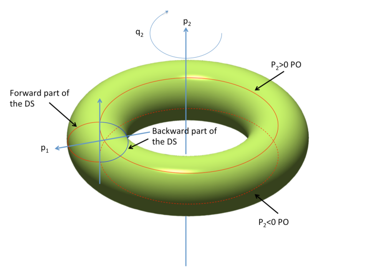
Figure 1: Topology of the DS for type 2 POs.

The 2 POs belong to the surface we are sampling. Taken individually, these two curves do not divide the 2-torus into two parts but the DS is divided into two parts when we considering both POs together: one part of the DS connects the $p_{2}>0$ PO with the $p_{2}<0$ PO on the left of the ellipse in momentum space and one part connects the $p_{2}>0$ PO with the $p_{2}<0$ PO on the right of the ellipse, see Fig. 1.

Trajectories cross the DS and the meaning of reaction for the constructed DS

Except for points on the NHIM, which belongs to the surface we are sampling, no trajectory initiated on the DS remains on the DS. Off the NHIM, the Hamiltonian vector field is everywhere transverse to the sampled surface, and every trajectory initiated on the DS has to leave the surface, i.e., trajectories cross the DS.

We have shown that the NHIM (or the 2 NHIMs for type 2 POs) divides the DS into two parts. One part of the DS intersects trajectories evolving from reactants to products and the other intersects trajectories evolving from products to reactants. Here, ‘reaction’ means crossing one of the two parts of the DS and the direction of the reaction, forward or backward, depends on which half of the DS the trajectory crosses.

To show that the vector field is nowhere tangent to the sampled surface, except on the NHIM, we must evaluate the flux form Ezra and Wiggins (2009a) associated with the Hamiltonian vector field through the DS on tangent vectors to the DS. The Hamiltonian vector field is not tangent to the DS if the flux form is nowhere zero on the DS, except at the NHIM. Details of this calculation are given in Appendix A.

III.2.2 Sampling of a Dividing Surface Attached to a NHIM for a 2 DoF Subsystem Plus an Elliptic Oscillator at a Fixed Total Energy

Under the assumptions introduced at the beginning of this section, the problem of the capture of an atom by a diatomic molecule at zero total angular momentum reduces to consideration of the dynamics of a 2 DoF subsystem and an elliptic oscillator. The algorithm presented for the sampling of a DS attached to a PO will be an essential element in our derivation of a sampling procedure of the DS in the case of a 3 DoF system composed of a 2 DoF subsystem plus an elliptic oscillator.

To begin, we need to understand the nature of the NHIM for this case. The motion for the elliptic oscillator (the diatomic vibration) consists of periodic orbits. For sufficiently small amplitude vibration (energy below the dissociation energy of the Morse like potential), these POs are stable. The NHIM for the full 3 DoF system (2 DoF subsystem plus 1 DoF elliptic oscillator) is obtained by considering the direct product of the NHIM for the 2 DoF subsytem with a PO of the elliptic oscillator. The NHIM for the 2 DoF subsytem, as we saw above, is just an unstable PO. If we consider a particular unstable PO for the 2 DoF subsystem and a particular PO for the elliptic oscillator, the structure obtained by the cartesian product of these 2 manifolds is a 2-dimensional torus. Every particular partitioning of the total energy $E$ between the 2 DoF subsystem and the elliptic oscillator corresponds to a particular 2-dimensional torus for the NHIM. The NHIM is then made up of a 1-parameter family of 2-dimensional tori, where the parameter of this family determines the distribution of energy between the 2 DoF subsystem and the elliptic oscillator.

Now that we have the structure of the NHIM it remains to construct the associated DS. Like the NHIM, the DS has a product structure: one part is associated with the 2 DoF subsystem and the other with the elliptic oscillator. For the elliptic oscillator all phase space points belong to a particular PO. For the 2 DoF subsystem the component of the DS consists of a DS attached to a PO as we described in Sec. III.2. If we consider one particular partitioning of the total energy $E$ between the 2 DoF subsystem and the elliptic oscillator, the portion of the DS associated with this distribution consists of the direct product of the DS associated with the unstable PO for the 2 DoF subsystem and the PO for the elliptic oscillator. The full DS is obtained by considering the DS for all possible partitions of the energy. The full DS is then foliated by ‘leaves’, where each leaf of the DS is associated with a particular partitioning of the energy.

To implement an algorithm for sampling the DS we need to determine the potential $V_{r}(r)$ for the diatomic molecule. This can be done by fixing a sufficiently large value of $R$, and fixing a value for $\theta$. In general, for large values of $R$ the potential $V(r,R,\theta)$ is isotropic, so any value of $\theta$ is sufficient. One can then use spline interpolation to obtain an analytical representation of the resulting Morse-like potential.

An algorithm to sample the DS in the case of a decoupled 2 DoF subsystem plus an elliptic oscillator is given as follows:

1. Consider a total energy $E$ for the full system.

2. Consider a particular partitioning of the total energy $E$ between the 2 DoF subsystem and the elliptic oscillator.

3. Sample points on the PO corresponding to the energy associated with the elliptic oscillator.

4. Sample points on the DS attached to the PO corresponding to the energy associated with the 2 DoF subsystem using the algorithm presented in the Sec. III.2.

5. Take the direct product the two sets of points obtained in the two previous steps.

6. Repeat the previous steps for many different energy distributions between the 2 DoF subsystem and the elliptic oscillator.

There is a subtlety related to the sampling procedure just described. The hyperbolic POs of the 2 DoF subsystem are associated with the centrifugal barrier arising in the atom-diatom Hamiltonian in Jacobi coordinates. Following the family of these POs it is found that as the energy decreases their location in the $(R,\theta)$ plane moves to larger and larger values of $R$. This suggests that the family goes asymptotically to a neutrally stable PO located at $R\to\infty$ neu . Reducing the energy in the 2 DoF subsystem therefore means locating POs at larger and larger distances in $R$, with longer and longer periods. Location of all such POs is clearly not possible numerically so that the sampling procedure must stop at some finite (small) energy in the diatomic vibration. The sampling procedure will nevertheless cover the DS, at least partially.

Alternatively, the energy in the diatomic vibration can simply be fixed at a specific value, as in the standard quasiclassical trajectory method (see, for example, the work of Bonnet et al. Bonnet and Rayez (1997) in which the energy of the diatomic vibration is fixed at the zero point energy). This approach then samples a particular leaf of the classical DS.

IV An Example: Recombination of the Ozone Molecule

The recombination reaction O $+$ O₂ $\rightarrow$ O₃ in the ozone molecule is known to exhibit an unconventional isotope effect Janssen et al. (2001). There is a large literature on this subject and many theoretical models have been proposed to identify the origin of this isotope effect Gao and Marcus (2001); Schinke et al. (2006); Janssen et al. (2001). One key to understanding the isotope effect in ozone is to model the recombination of an oxygen molecule with an oxygen atom. Marcus and coworkers have made a detailed study of the isotope effect in ozone Gao and Marcus (2001, 2002); Gao et al. (2002) and have used different models for the transition state in the recombination of ozone (tight and loose TS). In their studies, they used a variational version of RRKM theory Marcus (1952); Truhlar and Garrett (1984) (VTST) to locate the transition state. In order to obtain agreement between their calculations and experimental results they introduced parameters whose role consisted of correcting the statistical assumptions inherent in RRKM theory. Marcus and coworkers proposed several explanations for the physical origin of these parameters Gao and Marcus (2001, 2002); Gao et al. (2002) but their significance is still not fully understood. The deviation from statistical beheviour in the ozone molecule suggests that a dynamical study of the recombination reaction of ozone rather than a statistical model might shed light on the origin of the unconventional isotope effect. Such a study necessitates the use of DSs having dynamical significance, i.e., constructed in phase space.

To illustrate the construction of phase space DS for the capture of an atom by a diatomic molecule we apply the algorithms described in the previous section to the ozone recombination reaction. To attack this problem we require a PES for the ozone molecule which describes large amplitude motion. Schinke and coworkers produced the first accurate PES for ozoneSiebert et al. (2001, 2002). This PES exhibits a small barrier in the dissociation channel just below the asymptote for dissociation forming a van der Waals minimum and an associated ‘reef structure’. Recent ab initio calculations Tyuterev et al. (2013); Dawes et al. (2011, 2013) have however shown that the barrier is not present, and that the potential increases monotonically along the reaction coordinate (there is no saddle point along the reaction coordinate). Here, we use the PES produced by Tyuterev and coworkersTyuterev et al. (2013), which has recently been used to interpret experimental results Tyuterev et al. (2014).

In the following we treat the recombination of ozone molecule for the isotopic combination ¹⁶O¹⁶O¹⁶O by using two models. First, we treat the problem with a reduced 2 DoF model with zero total angular momentum, and then we look at the 3 DoF problem also with zero angular momentum.

IV.1 2 DoF model

The 2 DoF case is easily treated using the analysis of Sec. III.1 by freezing the diatomic vibration, i.e., ($r,p_{r}$) variables. We therefore fix the diatomic bond length at its equilibrium value, $r_{e}$, and set $p_{r}=0$. The dependence on $r$ in the coupling term of the potential then drops out and we have simply $V_{\text{coupling}}(R,\theta)=V_{\text{coupling}}(r=r_{e},R,\theta)$. The NHIM is obtained as previously by considering the uncoupled case with $V_{\text{coupling}}(R,\theta)=0$ and a hyperbolic equilibrium point in the ($R,p_{R}$) DoF, and is just a periodic orbit in the ($\theta,p_{\theta}$) DoF. This NHIM persists for non-zero coupling and consists of a periodic orbit where variables ($R,p_{R}$) and ($\theta,p_{\theta}$) are in general coupled.

The sampling of the DS follows the algorithm presented in Sec. III.2.1. We use the sampled points on the DS to initiate trajectories and follow the approach of the atom to the diatomic molecule. The resulting DS is a 2-dimensional surface in phase space whose points belong to the chosen energy surface. For our simulation we choose the total energy of 9200 cm^-1. The DS constructed from our algorithm is the first ‘portal’ the system has to cross in order for the atom to interact with the diatomic molecule. This DS is then the phase space realisation of the so-called Orbital or loose Transition State (OTS) Wiesenfeld et al. (2003); Wiesenfeld (2005). At the so-called Tight Transition State (TTS) Mauguière et al. (2014a), the coordinate $\theta$ undergoes constrained small oscillations. In our phase space setting, these TTS for a 2 DoF system are DSs attached to unstable POs. In the following the terms OTS and TTS are to be understood as synonymous with DSs constructed from NHIMs (POs for a 2 DoF system). An important mechanistic issue arising in modeling a reaction is to determine whether the reaction is mediated by an OTS or a TTS. However, in many situations both types of TS co-exist for the same energy and one has to understand the dynamical implications of the presence of these 2 types of TS.

In a recent work we analysed this question for a model ion-molecule system originally considered by Chesnavich Chesnavich et al. (1981); Chesnavich and Bowers (1982); Chesnavich (1986). We established a connection between the dynamics induced by the presence of these 2 types of TS and the phenomenon of roaming Mauguière et al. (2014a, b). Specifically, our phase space approach enabled us to define unambiguously a region of phase space bounded by the OTS and TTS which we called the roaming region. We were also able to classify trajectories initiated on the OTS into four different classes. These four classes were derived from two main categories. The main category consists of reactive trajectories. These trajectories start at the OTS and enter the roaming region between the OTS and TTS. They can then exhibit complicated dynamics in the roaming region and then react by crossing the TTS to form a bound triatomic molecule. Within this category we distinguish between roaming trajectories making some oscillations in the roaming region (oscillations were defined by the presence of turning points in $R$ coordinate) and direct trajectories that do not oscillate in the roaming region. The other main category of trajectories consists of trajectories that do not react and for which the atom finally separates from the diatomic molecule. Again we distinguish between trajectories which “roam” (making oscillations in the roaming region) and those that escape directly by bouncing off the hard wall at small values of $R$.

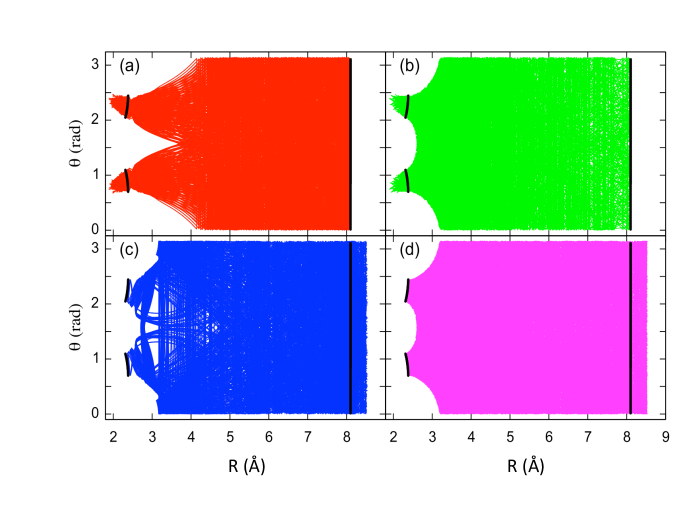
Figure 2: Trajectories propagated from the OTS for the 2 DoF model projected on configuration space. The black line at $R\simeq 8\text{\AA}$ is the PO from which the OTS is constructed. The short black curves at $R\simeq 2.5\text{\AA}$ are the POs from which the TTS are constructed. (a) Direct reactive trajectories. (b) Roaming reactive trajectories. (c) Direct non reactive trajectories. (d) Roaming non reactive trajectories.

For the ozone recombination problem reduced to a 2 DoF model we employ the same classification. Figure  2 shows the four classes of trajectories obtained by propagating incoming trajectories originated at the OTS. The black line at $R\simeq 8\text{\AA}$ is the PO from which the OTS is constructed. The two black curves at $R\simeq 2.5\text{\AA}$ are the two POs from which the two TTS are constructed. These two TTS correspond to the two channels by which the ozone molecule can recombine. For the case of ¹⁶O₃ the two channels reform the same ozone molecule but for different isotope composition these channels may lead to different ozone molecules. These trajectories show that the roaming phenomenon is at play in the ozone recombination problem. It would be very interesting to investigate how the roaming dynamics varies as the masses of the different oxygen atoms change, as this may provide new insight into the isotope effect in ozone recombination.

IV.2 3 DoF Model

We now consider the problem of ozone recombination in a 3 DoF model with zero total angular momentum. Addition of angular momentum DoF is in principle possible in our phase space description of reaction dynamics, but consideration of these DoF will increase the dimensionality of the problem and will require a more elaborate sampling procedure. Consideration of angular momentum in capture problems have been investigated by Wiesenfeld and coworkersWiesenfeld et al. (2003); Wiesenfeld (2004, 2005) and recently by MacKay and StrubMacKay and Strub (2015).

The construction of the DS for the OTS follows the procedure described in Sec. III.2.2. As explained in Sec. III.2.2 we cannot sample the full DS. In our simulation we sample one leaf of the DS by considering a single partitioning of the energy between the two DoF subsystem and the diatomic vibration. Here, for the sampling of the DS we fixed the diatomic length $r$ to its equilibrium value, and use the same value of the total energy as for the 2 DoF model, 9200 cm^-1.

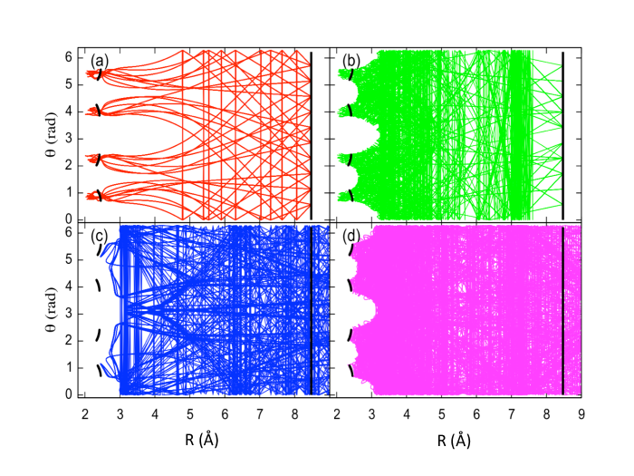
Figure 3: Trajectories propagated from the OTS for the 3 DoF model projected on configuration space. The black line at $R\simeq 8\text{\AA}$ is the projection of the PO from which the OTS is constructed. The short black curves at $R\simeq 2.5\text{\AA}$ are projections of POs that may be used as approximations of the TTS (see text). (a) Direct reactive trajectories. (b) Roaming reactive trajectories. (c) Direct non reactive trajectories. (d) Roaming non reactive trajectories.

The sampled points on the DS were again used to propagate trajectories, which are classified as previously into four classes. The result of the propagation is shown on Fig. 3. Again the black line at $R\simeq 8\,\text{\AA}$ represents the projection of the PO defining the OTS, while the two black curves at $R\simeq 2.5\,\text{\AA}$ are projections of POs. These POs are not strictly the proper phase space structures from which TTSs can be constructed as for a 3 DoF system the NHIM supporting a DS consists of a 1-parameter family of invariant 2-tori. Nevertheless, these POs give an idea of the approximate location of the projection of these structures into configuration space for ozone recombination. For the ozone problem it appears that they are very good approximation to the true NHIMs for the TTSs as we can see in Fig. 3 that none of the non reactive trajectories (panels (c) and (d)) extends beyond the projections of those POs on configuration space. The reason for that is presumably that for ozone the diatomic vibration is well decoupled from the 2 other DoF throughout the entire roaming region. This fact validates the reduced 2 DoF model presented above.

V Conclusion

In this paper we have examined the phase space structures that govern reaction dynamics in the absence of critical points on the PES. We showed that in the vicinity of hyperbolic invariant tori it is possible to define phase space dividing surfaces that are analogous to the dividing surfaces governing transition from reactants to products near a critical point of the PES.

We investigated the problem of capture of an atom by a diatomic molecule and showed that a normally hyperbolic invariant manifold (NHIM) exists at large atom-diatom distances, away from any critical points on the potential. This NHIM is the anchor for the construction of a DS in phase space, which is the entry ‘portal’ through which the atom has to pass in order to interact with the diatomic molecule. This DS defines the outer or loose TS (OTS) governing capture dynamics.

Making certain assumptions, we presented an algorithm for sampling an approximate capture DS. As an illustration of our methods we applied the algorithm to the recombination of the ozone molecule. We treated both 2 and 3 DoF models with zero total angular momentum. The co-existence of the OTS and TTS in ozone recombination means that roaming dynamics is observed for this reaction. Such roaming dynamics may have important consequences for the unconventional isotope effect in ozone formation.

Appendix A Verification that trajectories are transverse to the DS associated with the NHIM

To carry out this calculation we require a parametrization of the DS that will enable us derive expressions for tangent vectors to the DS. We can then compute the flux form and evaluate it on tangent vectors to the DS.

Parametrization of the DS

The DS is a 2-dimensional surface and therefore we require 2 parameters to parametrize it. These 2 parameters appear naturally from the sampling method, where we sample in the periodic coordinate $q_{2}$ and then in the momentum coordinate $p_{2}$. So, we use parameters ($p_{2},q_{2}$). Spline interpolation gives the function $q_{1}=q_{1}(q_{2})$ describing the dependence of coordinate $q_{1}$ on $q_{2}$ in the projection of the NHIM onto configuration space. The remaining momentum coordinate, $p_{1}$, is obtained by imposing the constant energy constraint $H=E$. The parametrization $\Phi$ of the DS can then be specified as:

$$\Phi(p_{2},q_{2})=\left(p_{1}=\pm\left[\left(E-V(q_{1}(q_{2}),q_{2})-\frac{p_{2}^{2}}{2I_{1}(q_{1}(q_{2}))}\right)2\mu\right]^{\frac{1}{2}},q_{1}(q_{2}),p_{2},q_{2}\right),$$ (16)

with $1/I_{1}=1/I+1/(\mu q_{1}^{2})$.

Tangent vectors to the DS are obtained by differentiating the parametrization with respect to the parameters $p_{2}$ and $q_{2}$:

$$u_{1} =\frac{\partial\Phi}{\partial p_{2}}=\left(\frac{\partial p_{1}}{\partial p_{2}},0,1,0\right)^{T}=\left(-\frac{\mu p_{2}}{I_{1}p_{1}(p_{2},q_{2})},0,1,0\right)^{T}$$ (17a)

$$u_{2} =\frac{\partial\Phi}{\partial q_{2}}=\left(\frac{\partial p_{1}}{\partial q_{2}},\frac{dq_{1}}{dq_{2}},0,1\right)^{T}=\left(-\frac{\left(\partial V/\partial q_{2}-\frac{p_{2}^{2}(dI_{1}/dq_{2})}{2I_{1}^{2}(q_{2})}\right)\mu}{p_{1}(p_{2},q_{2})},\frac{dq_{1}}{dq_{2}},0,1\right)^{T}.$$ (17b)

The flux form associated with the Hamiltonian vector field

For a 2 DoF system the phase space volume form $\Omega$ is expressed using the symplectic 2-form $\omega$ as follows:

$$\Omega=\frac{1}{2}\omega\wedge\omega.$$ (18)

The energy surface volume 3-form $\eta$ is defined by:

$$\Omega=dH\wedge\eta.$$ (19)

The Hamiltonian vector field is:

$$X_{H}=\left(-\frac{\partial H}{\partial q_{1}},\frac{\partial H}{\partial p_{1}},-\frac{\partial H}{\partial q_{2}},\frac{\partial H}{\partial p_{2}}\right).$$ (20)

The symplectic 2-form $\omega$ when applied to an arbitrary vector $\xi$ and the vector field $X_{H}$ gives:

$$\omega(\xi,X_{H})=dH(\xi).$$ (21)

The flux 2-form $\varphi$ through a codimension one surface in the energy surface (that is a 2-dimensional surface like our DS) is simply given by the interior product of the energy surface volume form $\eta$ with the Hamiltonian vector field:

$$\varphi=i_{X_{H}}\eta.$$ (22)

To compute $\varphi$ we take two vectors $\xi_{1}$ and $\xi_{2}$ tangent to the DS and a vector $\xi_{3}$ such that $dH(\xi_{3})\neq 0$. First we note that the volume form $\Omega$ when applied to $\xi_{1}$, $\xi_{2}$, $\xi_{3}$ and $X_{H}$ gives:

$$\Omega(\xi_{1},\xi_{2},\xi_{3},X_{H}) =\omega(\xi_{1},\xi_{2})\omega(\xi_{3},X_{H})-\omega(\xi_{1},\xi_{3})\omega(\xi_{2},X_{H})+\omega(\xi_{1},X_{H})\omega(\xi_{2},\xi_{3})$$ (23a)

$$=\omega(\xi_{1},\xi_{2})dH(\xi_{3})-\omega(\xi_{1},\xi_{3})dH(\xi_{2})+\omega(\xi_{2},\xi_{3})dH(\xi_{1})$$ (23b)

$$=\omega(\xi_{1},\xi_{2})dH(\xi_{3}).$$ (23c)

The last line follows since $\xi_{1}$ and $\xi_{2}$ are tangent vectors to the DS and therefore $dH(\xi_{i})=0$ for $i=1,2$. Also, we have $dH(X_{H})=0$ as $X_{H}$ is a tangent vector field to the energy surface. From the definition of the energy surface volume form we have:

$$\Omega(\xi_{1},\xi_{2},\xi_{3},X_{H}) =dH\wedge\eta(\xi_{1},\xi_{2},\xi_{3},X_{H})$$ (24a)

$$=dH(\xi_{1})\eta(\xi_{2},\xi_{2},X_{H})+dH(\xi_{2})\eta(\xi_{1},\xi_{3},X_{H})$$

$$+dH(\xi_{3})\eta(\xi_{1},\xi_{2},X_{H})+dH(X_{H})\eta(\xi_{1},\xi_{2},\xi_{3})$$ (24b)

$$=dH(\xi_{3})\eta(\xi_{1},\xi_{2},X_{H}).$$ (24c)

Since $\varphi(\xi_{1},\xi_{2})=i_{X_{H}}\eta(\xi_{1},\xi_{2})=\eta(\xi_{1},\xi_{2},X_{H})$, it then follows from (23) and (24) that:

$$dH(\xi_{3})\omega(\xi_{1},\xi_{2})=dH(\xi_{3})\,i_{X_{H}}\eta(\xi_{1},\xi_{2})$$ (25)

and

$$\varphi=i_{X_{H}}\eta(\xi_{1},\xi_{2})=\omega(\xi_{1},\xi_{2}).$$ (26)

The flux form through the DS is simply the symplectic 2-form applied to tangent vectors of the DS.

Condition for non-tangency of the Hamiltonian vector field

To check that the vector field is not tangent to the DS (i.e. trajectories cross the DS) we need to evaluate the flux form on tangent vectors to the DS.

The calculation we need to carry out is the following:

$$\omega(u_{1},u_{2}) =(dp_{1}\wedge dq_{1}+dp_{2}\wedge dq_{2})(u_{1},u_{2})$$ (27a)

$$=(u_{1}^{p_{1}}u_{2}^{q_{1}}-u_{1}^{q_{1}}u_{2}^{p_{1}})+(u_{1}^{p_{2}}u_{2}^{q_{2}}-u_{1}^{q_{2}}u_{2}^{p_{2}})$$ (27b)

$$=-\frac{\mu p_{2}}{I_{1}p_{1}}\frac{dq_{1}}{dq_{2}}+1$$ (27c)

The flux through the DS is then zero whenever:

$$\frac{dq_{2}}{dq_{1}}=\frac{p_{2}/I_{1}}{p_{1}/\mu}=\frac{\dot{q_{2}}}{\dot{q_{1}}}$$ (28)

That is, the ratio of velocities corresponds precisely to the phase point being on the NHIM (PO).

References

- Mezey (1987) P. G. Mezey, Potential Energy Hypersurfaces (Elsevier, Amsterdam, 1987).
- Wales (2003) D. J. Wales, Energy Landscapes (Cambridge University Press, Cambridge, 2003).
- Chandler (1978) D. Chandler, J. Chem. Phys. 68, 2959 (1978).
- Berne et al. (1982) B. J. Berne, N. DeLeon, and R. O. Rosenberg, J. Phys. Chem. 86, 2166 (1982).
- Davis and Gray (1986) M. J. Davis and S. K. Gray, J. Chem. Phys. 84, 5389 (1986).
- Gray and Rice (1987) S. K. Gray and S. A. Rice, J. Chem. Phys. 86, 2020 (1987).
- Minyaev (1991) R. M. Minyaev, J. Struct. Chem. 32, 559 (1991).
- Minyaev (1994) R. M. Minyaev, Russ. Chem. Rev. 63, 883 (1994).
- Baer and Hase (1996) T. Baer and W. L. Hase, Unimolecular Reaction Dynamics (Oxford University Press, New York, 1996).
- Leitner (1999) D. M. Leitner, Int. J. Quantum Chem. 75, 523 (1999).
- Waalkens et al. (2004) H. Waalkens, A. Burbanks, and S. Wiggins, J. Chem. Phys. 121, 6207 (2004).
- Carpenter (2005) B. K. Carpenter, Ann. Rev. Phys. Chem. 56, 57 (2005).
- Joyeux et al. (2005) M. Joyeux, S. Y. Grebenshchikov, J. Bredenbeck, R. Schinke, and S. C. Farantos, Adv. Chem. Phys. 130 A, 267 (2005).
- Ezra et al. (2009) G. S. Ezra, H. Waalkens, and S. Wiggins, J. Chem. Phys. 130, 164118 (2009).
- Pettini (2007) M. Pettini, Geometry and Topology in Hamiltonian Dynamics and Statistical Mechanics (Springer, New York, 2007).
- Kastner (2008) M. Kastner, Rev. Mod. Phys. 80, 167 (2008).
- Arnold et al. (2006) V. I. Arnold, V. V. Kozlov, and A. I. Neishtadt, Mathematical Aspects of Classical and Celestial Mechanics (Springer, New York, 2006).
- Wiggins (2003) S. Wiggins, Introduction to Applied Nonlinear Dynamical Systems and Chaos (Springer-Verlag, New York, 2003), 2nd ed.
- Farantos (2014) S. C. Farantos, Nonlinear Hamiltonian Mechanics Applied to Molecular Dynamics: Theory and computational methods for understanding molecular spectroscopy and chemical reactions (Springer, 2014).
- Lichtenberg and Lieberman (1992) A. J. Lichtenberg and M. A. Lieberman, Regular and Chaotic Dynamics (Springer Verlag, New York, 1992), 2nd ed.
- (21) Consider a potential energy function that is a function of coordinates . (Coordinates describing translation and rotation are excluded.) At a non-degenerate critical point of , where , , the Hessian matrix has nonzero eigenvalues. The index of the critical point is the number of negative eigenvalues.
- Komatsuzaki and Berry (2000) T. Komatsuzaki and R. S. Berry, J. Mol. Struct. THEOCHEM 506, 55 (2000).
- Wiggins et al. (2001) S. Wiggins, L. Wiesenfeld, C. Jaffé, and T. Uzer, Physical Review Letters 86, 5478 (2001).
- Uzer et al. (2002) T. Uzer, C. Jaffé, J. Palacián, P. Yanguas, and S. Wiggins, Nonlinearity 15, 957 (2002).
- Waalkens et al. (2008) H. Waalkens, R. Schubert, and S. Wiggins, Nonlinearity 21, R1 (2008).
- Heidrich and Quapp (1986) D. Heidrich and W. Quapp, Theor. Chim. Acta 70, 89 (1986).
- Ezra and Wiggins (2009a) G. S. Ezra and S. Wiggins, J. Phys. A 42, 205101 (2009a).
- Haller et al. (2010) G. Haller, J. Palacian, P. Yanguas, T. Uzer, and C. Jaffé, Comm. Nonlinear Sci. Num. Simul. 15, 48 (2010).
- Shida (2005) N. Shida, Adv. Chem. Phys. 130 B, 129 (2005).
- Ezra and Wiggins (2009b) G. Ezra and S. Wiggins, Journal of Physics A: Mathematical and Theoretical 42, 205101 (2009b).
- Collins et al. (2011) P. Collins, G. S. Ezra, and S. Wiggins, J. Chem. Phys. 134, 244105 (2011).
- Mauguiere et al. (2013) F. Mauguiere, P. Collins, G. Ezra, and S. Wiggins, J. Chem. Phys. 138, 134118 (2013).
- Wiggins (1990) S. Wiggins, Physica D 44, 471 (1990).
- Wiggins (1994) S. Wiggins, Normally hyperbolic invariant manifolds in dynamical systems (Springer-Verlag, 1994).
- Waalkens and Wiggins (2004) H. Waalkens and S. Wiggins, J. Phys. A: Math. Gen. 37, L435 (2004).
- Li et al. (2009) C.-B. Li, M. Toda, and T. Komatsuzaki, J. Chem. Phys. 130, 124116 (2009).
- Inarrea et al. (2011) M. Inarrea, J. F. Palacian, A. I. Pascual, and J. P. Salas, J. Chem. Phys. 135, 014110 (2011).
- Mauguière et al. (2013) F. A. L. Mauguière, P. Collins, G. S. Ezra, and S. Wiggins, Int. J. Bifurcat. Chaos 23 (2013).
- MacKay and Strub (2014) R. S. MacKay and D. C. Strub, Nonlinearity 27, 859 (2014).
- Sun et al. (2002) L. P. Sun, K. Y. Song, and W. L. Hase, Science 296, 875 (2002).
- Townsend et al. (2004) D. Townsend, S. A. Lahankar, S. K. Lee, S. D. Chambreau, A. G. Suits, X. Zhang, J. Rheinecker, L. B. Harding, and J. M. Bowman, Science 306, 1158 (2004).
- Bowman (2006) J. M. Bowman, PNAS 103, 16061 (2006).
- Lopez et al. (2007) J. G. Lopez, G. Vayner, U. Lourderaj, S. V. Addepalli, S. Kato, W. A. Dejong, T. L. Windus, and W. L. Hase, J. Am. Chem. Soc. 129, 9976 (2007).
- Heazlewood et al. (2008) B. R. Heazlewood, M. J. T. Jordan, S. H. Kable, T. M. Selby, D. L. Osborn, B. C. Shepler, B. J. Braams, and J. M. Bowman, PNAS 105, 12719 (2008).
- Shepler et al. (2008) B. C. Shepler, B. J. Braams, and J. M. Bowman, J. Phys. Chem. A 112, 9344 (2008).
- Suits (2008) A. G. Suits, Acc. Chem. Res. 41, 873 (2008).
- Bowman and Shepler (2011) J. M. Bowman and B. C. Shepler, Ann. Rev. Phys. Chem. 62, 531 (2011).
- Bowman and Suits (2011) J. M. Bowman and A. G. Suits, Phys. Today 64, 33 (2011).
- Bowman (2014) J. M. Bowman, Molecular Physics 112, 2516 (2014).
- Wiesenfeld et al. (2003) L. Wiesenfeld, A. Faure, and T. Johann, J. Phys. B 36, 1319 (2003).
- Wiesenfeld (2004) L. Wiesenfeld, Few Body Syst. 34, 163 (2004).
- Wiesenfeld (2005) L. Wiesenfeld, Adv. Chem. Phys. 130 A, 217 (2005).
- Chesnavich et al. (1981) W. J. Chesnavich, L. Bass, T. Su, and M. T. Bowers, J. Chem. Phys. 74, 2228 (1981).
- Chesnavich and Bowers (1982) W. J. Chesnavich and M. T. Bowers, Theory of Ion-Neutral Interactions: Application of Transition State Theory Concepts to Both Collisional and Reactive Properties of Simple Systems (Pergamon Press, 1982).
- Chesnavich (1986) W. J. Chesnavich, J. Chem. Phys. 84, 2615 (1986).
- Mauguière et al. (2014a) F. A. L. Mauguière, P. Collins, G. S. Ezra, S. C. Farantos, and S. Wiggins, Chem. Phys. Lett. 592, 282 (2014a).
- Mauguière et al. (2014b) F. A. L. Mauguière, P. Collins, G. S. Ezra, S. C. Farantos, and S. Wiggins, J. Chem. Phys. 140, 134112 (2014b).
- Mauguière et al. (2014c) F. A. L. Mauguière, P. Collins, G. S. Ezra, S. C. Farantos, and S. Wiggins, Theor. Chem. Acc. 133, 1507 (2014c).
- Mauguière et al. (2015) F. A. L. Mauguière, P. Collins, Z. C. Kramer, B. K. Carpenter, G. S. Ezra, S. C. Farantos, and S. Wiggins, J. Phys. Chem. Lett. 6, 4123 (2015).
- Janssen et al. (2001) C. Janssen, J. Guenther, K. Mauersberger, and D. Krankowsky, Phys. Chem. Chem. Phys. 3, 4718 (2001).
- Gao and Marcus (2001) Y. Q. Gao and R. A. Marcus, Science 293, 259 (2001).
- Gao and Marcus (2002) Y. Q. Gao and R. A. Marcus, J. Chem. Phys. 116, 137 (2002).
- Gao et al. (2002) Y. Q. Gao, W.-C. Chen, and R. A. Marcus, J. Chem. Phys. 117, 1536 (2002).
- Schinke et al. (2006) R. Schinke, S. Y. Grebenshchikov, M. V. Ivanov, and P. Fleurat-Lessard, Annu. Rev. Phys. Chem. 57, 625 (2006).
- Bolotin and Treschev (2000) S. V. Bolotin and D. V. Treschev, Regul. Chaotic Dyn. 5, 401 (2000).
- Meyer et al. (2009) K. R. Meyer, G. R. Hall, and D. Offin, Introduction to Hamiltonian Dynamical Systems and the N-Body Problem, vol. 90 of Applied Mathematical Sciences (Springer, Heidelberg, New York, 2009), 2nd ed.
- Stone (2013) A. Stone, The Theory of Intermolecular Forces (Oxford University Press, Great Clarendon Street, Oxford, ox2 6dp, United Kingdom, 2013).
- Farantos (1998) S. C. Farantos, Comput. Phys. Commun. 108, 240 (1998).
- Press et al. (1992) W. H. Press, B. P. Flannery, S. A. Teukolsky, and W. T. Vetterling, Numerical Recipes in FORTRAN: The Art of Scientific Computing (Cambridge University Press, Cambridge, 1992).
- (70) A periodic orbit is said to be neutrally stable if all of its Lyapunov exponents are zero.
- Bonnet and Rayez (1997) L. Bonnet and J. Rayez, Chem. Phys. Lett. 277, 183 (1997).
- Marcus (1952) R. A. Marcus, J. Chem. Phys. 20, 359 (1952).
- Truhlar and Garrett (1984) D. Truhlar and B. Garrett, Ann. Rev. Phys. Chem. 35, 159 (1984).
- Siebert et al. (2001) R. Siebert, R. Schinke, and M. Bittererová, Phys. Chem. Chem. Phys. 3, 1795 (2001).
- Siebert et al. (2002) R. Siebert, P. Fleurat-Lessard, R. Schinke, M. Bittererová, and S. C. Farantos, J. Chem. Phys. 116, 9749 (2002).
- Tyuterev et al. (2013) V. G. Tyuterev, R. V. Kochanov, S. A. Tashkun, F. Holka, and P. G. Szalay, J. Chem. Phys. 139, 134307 (2013).
- Dawes et al. (2011) R. Dawes, P. Lolur, J. Ma, and H. Guo, J. Chem. Phys. 135, 081102 (2011).
- Dawes et al. (2013) R. Dawes, P. Lolur, A. Li, B. Jiang, and H. Guo, J. Chem. Phys. 139, 201103 (2013).
- Tyuterev et al. (2014) V. G. Tyuterev, R. Kochanov, A. Campargue, S. Kassi, D. Mondelain, A. Barbe, E. Starikova, M.-R. De Backer, P. G. Szalay, and S. Tashkun, Phys. Rev. Lett. 113, 143002 (2014).
- MacKay and Strub (2015) R. S. MacKay and D. C. Strub, ArXiv e-prints (2015), eprint 1501.00266.