Gradient Estimation with Simultaneous Perturbation and Compressive Sensing
(Gradient Estimation)
Abstract
We propose a scheme for finding a “good” estimator for the gradient of a function on a high-dimensional space with few function evaluations. Often such functions are not sensitive in all coordinates and the gradient of the function is almost sparse. We propose a method for gradient estimation that combines ideas from Spall’s Simultaneous Perturbation Stochastic Approximation with compressive sensing. Applications to estimating gradient outer product matrix as well as standard optimization problems are illustrated via simulations.
Keywords: Gradient estimation; Compressive sensing; Sparsity; Gradient descent; Gradient outer product matrix.
1 Introduction
Estimating the gradient of a given function (with or without noise) is often an important part of problems in reinforcement learning, optimization and manifold learning. In reinforcement learning, policy-gradient methods are used to obtain an unbiased estimator for the gradient. The policy parameters are then updated with increments proportional to the estimated gradient [27]. The objective is to learn a locally optimum policy. REINFORCE and PGPE methods (policy gradients with parameter-based exploration) are popular instances of this approach (See [35] for details and comparisons, [13] for a survey on policy gradient methods in the context of actor-critic algorithms). In manifold learning, various finite difference methods have been explored for gradient estimation [21], [32]. The idea is to use the estimated gradient to find the lower dimensional manifold where the given function actually lives. Optimization, i.e. finding maximum or minimum of a function, is a ubiquitous problem that appears in many fields wherein one seeks zeroes of the gradient. But the gradient itself might be hard to compute. Gradient estimation techniques prove particularly useful in such scenarios.
A further theoretical justification is facilitated by the results of [1]. In [1], it was shown that given a connected and locally connected metric probability space (i.e., is a compact metric space with metric and is a probability measure on the Borel -algebra of ), under suitable conditions, any function is close (in ) to a function on a lower dimensional space. As a special case, a similar fact can be proved for real-values -Lipschitz functions on with metric (See Theorem 1.2 in [1]). This suggests that sparse gradients can be expected for functions on high dimensional spaces with adequate regularity conditions.
Over the years gradient estimation has also become an interesting problem in its own right. One would expect that the efficiency of a given method for gradient estimation also depends on the properties of function . We consider one such class of problems in this paper. Suppose we have a continuously differentiable function where is large, such that the gradient lives mostly in a lower dimensional subspace. This means that one can throw out most of the coordinates of in a suitable local basis without incurring too much error. In this case, computing is clearly a waste of means. Dimensionality reduction techniques for optimization problems is an active area of research and several useful methods for this have been developed in the mathematical and engineering community [16], [34]. If in addition the function evaluations are expensive, most gradient estimation methods become inefficient. Such is the case, e.g., if a single function evaluation is the output of a large time consuming simulation. This situation our specific focus. The problem of expensive function evaluations does not seem to have attracted much attention in machine learning literature. However, there has been quite a lot of work on optimization of functions with expensive evaluation. Most methods, however, focus on learning a good surrogate for the original function (See [15], [23], [25]).
To handle the first issue, ideas from compressive sensing can be applied. Compressive sensing theory tells us that an -sparse vector can be reconstructed from measurements. This means that one does not need the information about in all directions, a much smaller number of measurements would suffice. These ideas are frequently used in signal as well as image processing (see, e.g., [9, 10]). To remedy the latter difficulty, we use an idea from Simultaneous Perturbation Stochastic Approximation (SPSA) due to Spall [26], viz., the Simultaneous Perturbation (SP).
We begin by explaining the proposed method for gradient estimation. Important ideas and results from compressive sensing and SPSA that are relevant to this work are discussed in section 2.1 and section 2.2 respectively. We state the main result in section 2.3. Section 3 consists of applications to manifold learning and optimization with simulated examples.
Some notational preliminaries are as follows. By we denote the usual Euclidean norm in as well as the Frobenius norm for matrices over . Throughout, ‘a.s.’ stands for ‘almost surely’, i.e., with probability one.
2 Gradient Estimation: Combining Compressive Sensing and SP
As mentioned above, if function evaluations are expensive, SP works well to avoid the problem of computing function multiple times. However, if the gradient is sparse it makes sense to use the ideas of compressive sensing to our advantage. Combining these two techniques helps us overcome the problem of too many function evaluations and also exploit the sparse structure of the gradient. The idea is to use SP to get sufficient number of observations to be able to recover the gradient via -minimization. We describe the method in detail in the following sub-sections.
2.1 Compressive Sensing
Assume that is an approximately sparse vector. The idea of compressive sensing is based on the fact that typically a sparse vector contains much less information or complexity than its apparent dimension. Therefore one should be able to reconstruct with considerable accuracy with much less information than that of order . We will make these ideas more precise in the forthcoming discussion on compressive sensing. We state all the results for vectors in . All of these results also hold for vectors over . We start by defining what we mean by sparse vectors.
Definition 2.1 (Sparsity).
The support of a vector is defined as:
where . The vector is called -sparse if at most of its entries are nonzero, i.e., if
We assume that the observed data is related to the original vector via for some matrix , where . In other words, we have a linear measurement process for observing . The theory of compressive sensing tells us that if is sparse, then it can recovered from by solving a convex optimization problem. In particular, given a suitable matrix and appropriate , the following -minimization problem recovers exactly.
| (1) |
where are the observations. These ideas were introduced by E. Candes and T. Tao in their seminal paper on near-optimal signal reconstruction [6]. In this paper, the authors proved that the matrices suitable for the recovery need to have what is called the restricted isometry property (RIP). A large class of random matrices satisfy the RIP with quantifiable ‘high probability’ and are therefore suitable for reconstruction via -minimization. In particular, subgaussian matrices have been shown to have RIP with high probability and are suitable for the aforementioned reconstruction scheme for . This gives the explicit relationship between the sparsity level , the dimension of the original vector and the dimension of the observed data . In recent times some work has been done to construct deterministic matrices with this restricted isometry property [2]. The current known lower bound on for deterministic matrices is of the order of where is the sparsity. Thus random matrices are a better choice for linear measurement for reconstruction via compressive sensing.
For the scope of this paper, we consider robust recovery options using Gaussian random matrices, i.e., matrices whose entries are realizations of independent standard normal random variables.
Remark 1.
Matrices with more structure like random partial Fourier matrix or in general bounded orthonormal systems can also be used as meaurement matrices for compressive sensing techniques. Given a random draw of such a matrix with associated constant , a fixed -sparse vector can be reconstructed via -minimization with high probability provided . For more details on random sampling matrices in compressive sensing see chapter 12 of [11].
The crucial point here is that it is enough that the given vector is sparse in some basis. A more detailed discussion on various aspects of compressive sensing can be found in [11]. In real-life situations the measurements are almost always noisy. It may also happen that the original vector is not sparse but is close to a sparse vector. In other words, we would like the reconstruction scheme to be robust and stable. Theorem 9.13 of [11] gives explicit error bounds for stable and robust recovery where is a subgaussian matrix. The bound is expressed in terms of , the distance of from the nearest -sparse vector, and the measurement error. See [7],[8] and [17] for more on robust and stable recovery via compressive sensing.
We assume that our observations are noisy. The following theorem gives an error bound on the reconstruction from noisy measurements using a Gaussian matrix.
Theorem 2.2 (Theorem 9.20 in [11]).
Let be a random draw of a Gaussian random matrix and be a -sparse vector. Let be noisy measurements of such that . If for and some ,
| (2) |
then with probability at least every that minimizes subject to approximates with -error
See Theorem 9.29 in [11] for a statement for stable and robust recovery via Gaussian matrices.
2.2 Simultaneous Perturbation Stochastic Approximation
As discussed above we have a fairly good reconstruction of a sparse gradient given a sufficient number of observations . However, as mentioned before, the problem often is the unavailability of these observations. Even though observations for are not readily available, one may compute ’s using the available information, that is, noisy measurements of the function . Note that we have, however, assumed that the function evaluations are computationally expensive. We will now address this issue of estimating with low computational overheads.
Let denote the coordinate direction for . We consider the finite difference approximation
where and . By Taylor’s theorem, the error of estimation is where denotes the Hessian. This estimate requires function evaluations. Replacing the ‘two sided differences’ above by ‘one sided differences’ reduces this to , which is still large for large . Given that we have assumed to be such that the function evaluations are computationally expensive, an alternative method is desirable. We use the method devised by Spall [26] in the context of stochastic gradient descent, known as Simultaneous Perturbation Stochastic Approximation (SPSA).
Recall the stochastic gradient descent scheme [5]
| (3) |
where:
-
•
is a square-integrable martingale difference sequence, viz., a sequence of zero mean random variables with finite second moment satisfying
i.e., it is uncorrelated with the past. We assume that it also satisfies
(4) -
•
are step-sizes satisfying
(5)
The term in square bracket in (3) stands for a noisy measurement of the gradient. Under mild technical conditions, can be shown to converge a.s. to a local minimum of [5]. The idea is that the incremental adaptation due to the slowly decreasing step-size averages out the noise , rendering this a close approximation of the classical gradient descent with vanishing error [5]. In practice the noisy gradient is often unavailable and one has to use an approximation thereof using noisy evaluations of , e.g., the aforementioned finite difference approximations, which lead to the Kiefer-Wolfowitz scheme. That is where the SP scheme comes in. We describe this next.
Let be i.i.d. zero mean random variables such that
-
•
is independent of .
-
•
.
Then by Taylor’s theorem, we have that for :
| (6) |
Note that since ’s are i.i.d. zero mean random variables, we have for ,
Hence for the purpose of stochastic gradient descent, the second term in (6) acts as a zero mean noise (i.e., martingale difference) term that can be clubbed with as martingale difference noise and gets averaged out by the iteration. This serves our purpose, since the above scheme requires only two function evaluations per iterate given by
Our idea is to generate according to the scheme discussed above.
It should be mentioned that Spall also introduced another approximation based on a single function evaluation (see, e.g., [5], Chapter 10). But this suffers from numerical issues due to the ‘small divisor’ problem, so we do not pursue it here.
2.3 Main result
As mentioned in the introduction, the idea is to combine the SP and compressive sensing to obtain a sparse approximation of . Note that while SP gives an estimate with zero-mean error, the final estimate of gradient obtained after compressive sensing may not be unbiased. To avoid the error from piling up we need to average out the error at SP stage. We propose the following algorithm for estimating gradient of . Let denote the row vectors of .
Initialization:
random Gaussian matrix.
Output: estimated gradient .
The following theorem states that with high probability such an approximation is “close” to the actual gradient.
Theorem 2.3.
Proof.
Let be a Gaussian matrix such that satisfies (2). Then, following the same idea as in (6), we have:
| (7) | |||||
So we get
| (8) |
where we quantify the ‘error’ below.
The above computation is carried out times independently, keeping the matrix fixed and choosing the random vector according to the distribution defined in section 2.2. The reason for this additional averaging is as follows. The reconstruction in compressive sensing need not give an unbiased estimate, since it performs a nonlinear (minimization) operation. Thus it is better to do some pre-processing of the SP estimate (which is nearly, i.e., modulo the term, unbiased) to reduce its variance. We do so by repeating it times with independent perturbations and taking its arithmetic mean. This may seem to defeat our original objective of reducing function evaluations, but the required to get reasonable error bounds is not large as our analysis shows later, and the computational saving is still significant (see ‘Remark 2’ below).
Denote by the measurement obtained at iteration of SP. The error for a single iteration is given by
Denote by . So, are zero-mean conditionally (given past iterates) independent random variables.
The error vector after iterations is given by
| (9) | |||||
In order to apply the ideas from compressive sensing as in Theorem 2.2, we need to have a bound on the error . This is obtained as follows. Let be a constant such that the term above is bounded in absolute value by . can, e.g., be a bound on by the mean value theorem, where we use the Frobenius norm. Choose and . Then, by Hoeffding’s inequality we have,
| (10) | |||||
Remark 2.
Note that the minimum number of iterations of SP required to obtain a “good” estimate of is given by
for a suitable constant .
The above can now be used as an effective gradient in various problems involving gradients of high-dimensional functions. Two such applications are discussed in the next section.
3 Applications
We consider the applications of our method to manifold learning and optimization problems. The gradient estimates obtained using our method can be used to estimate the gradient outer product matrix or can be plugged into an optimization scheme. In the former case, along with an example, we also provide error bounds on the estimated and actual gradient outer product matrix. For the latter case, we look at an example and provide suitable modifications to existing algorithms to achieve faster convergence. Algorithm 1 below which is based on Theorem 2.3, is used for gradient estimation.
There are various algorithms available for carrying out the -minimization. A detailed discussion of these algorithms can be found in [12], Chapter 15 of [11]. Here we use the homotopy method.
Initialization:
random Gaussian matrix.
Output: estimated gradient .
Here denotes the -recovery from observations and Gaussian random matrix using the homotopy method. All the simulations were performed on MATLAB using the available toolbox for -minimization (Berkeley database: http://www.eecs.berkeley.edu/ yang/software/ l1benchmark/).
Consider a function given by where, is -dimensional matrix with non-zero elements per row. Let be a random Gaussian matrix that is used for measurement. We consider measurements.
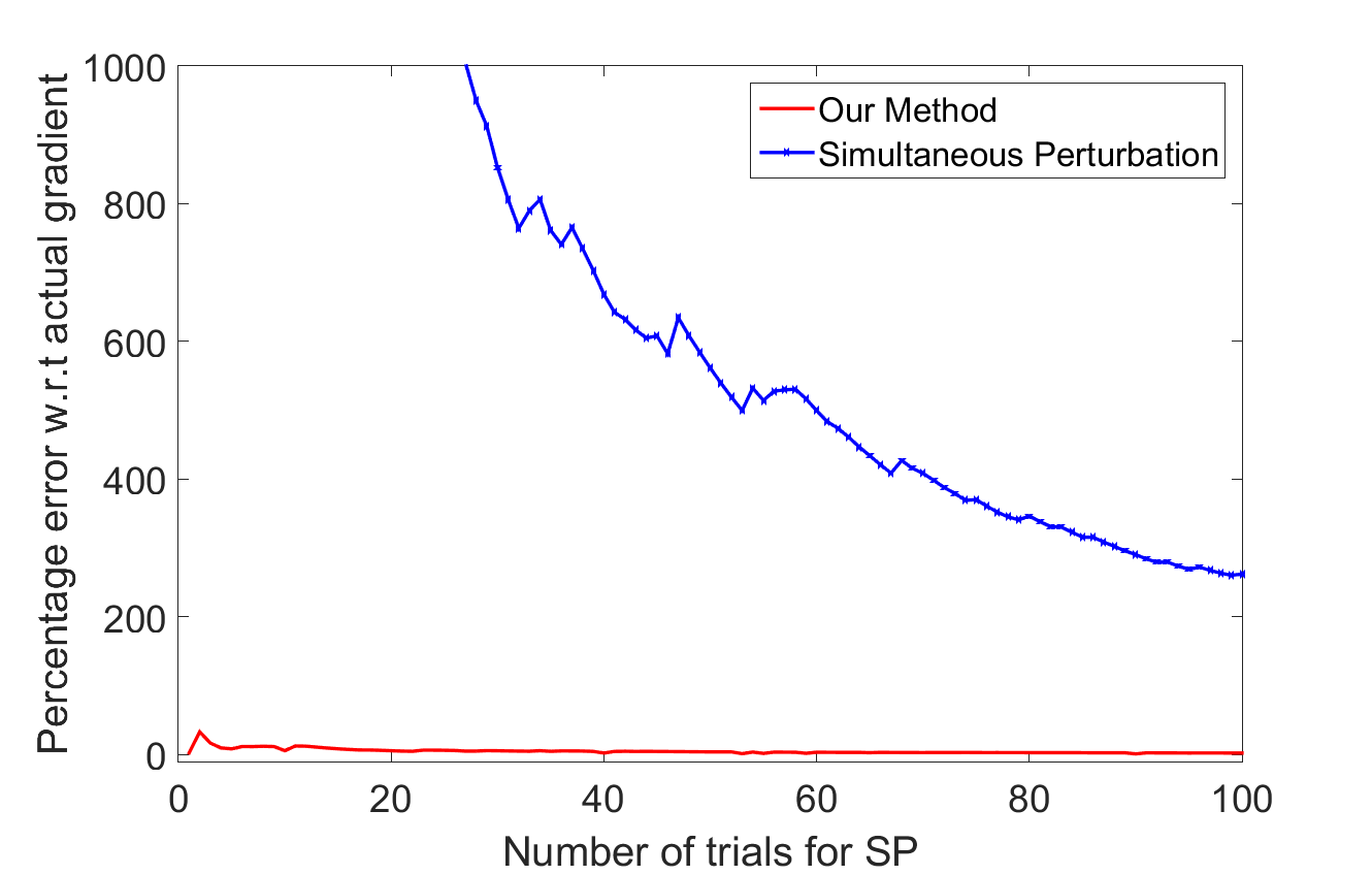
Figure 1 shows the performance of the proposed method with varying number of SP iterations.
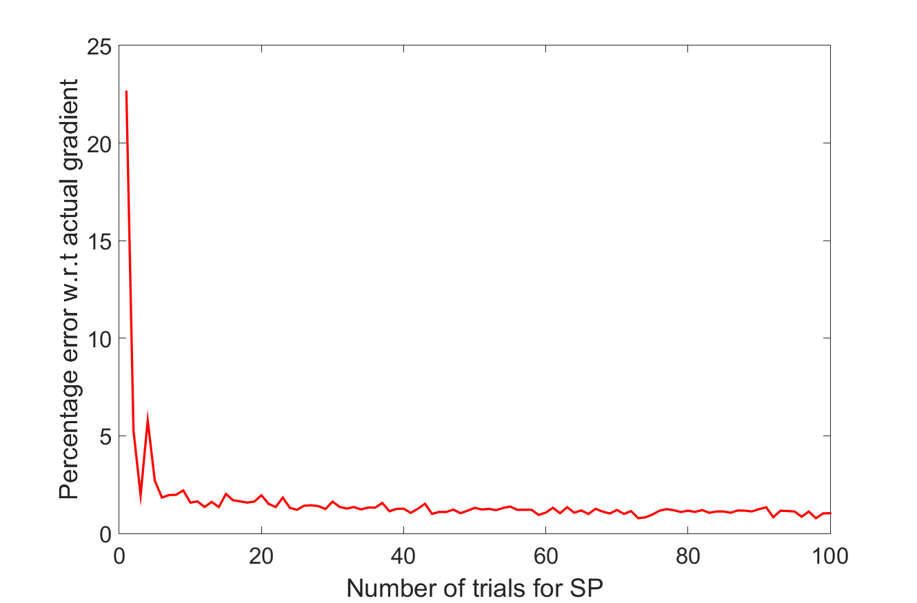
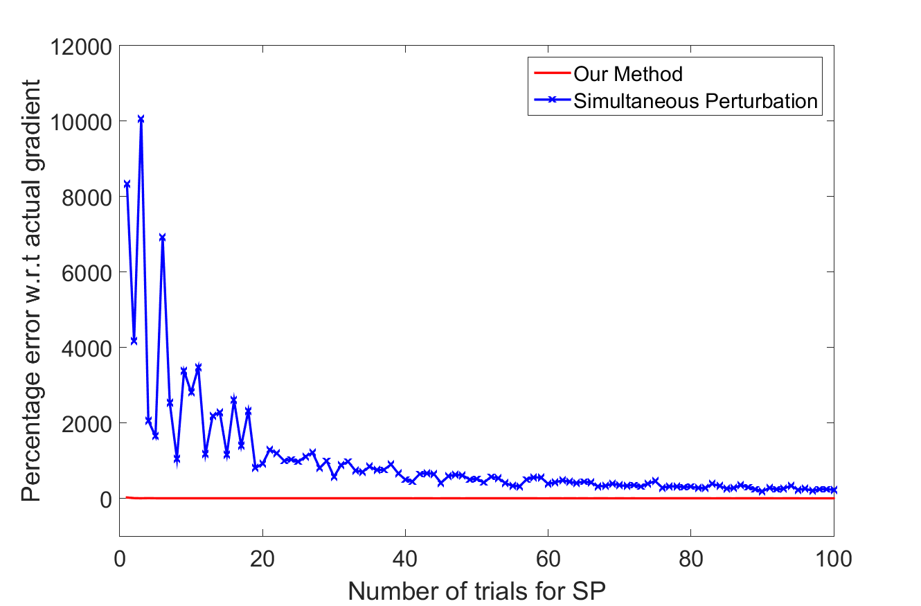
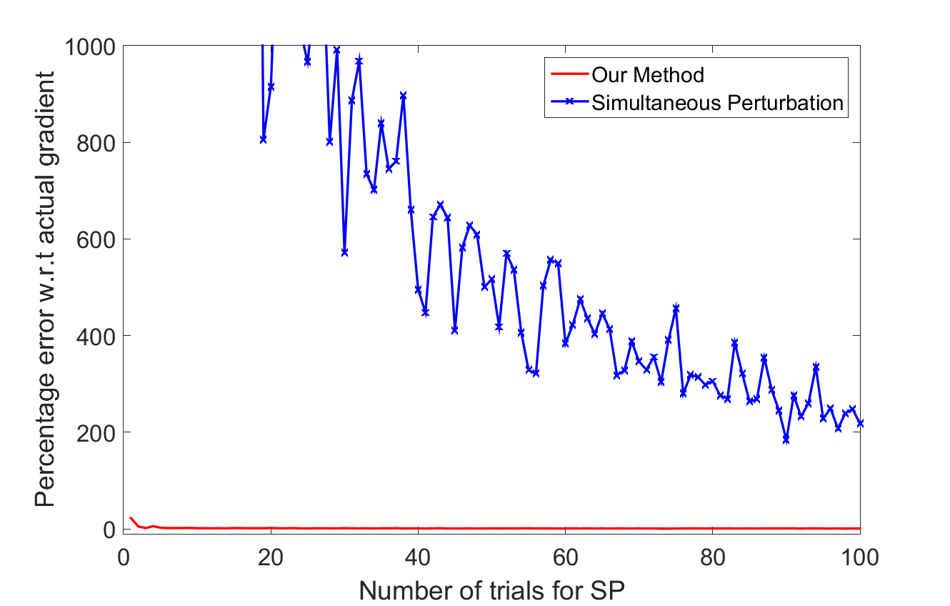
Figure 3 and 3 show the comparison between our method and naive SP for estimating gradient with gradually increasing number of iterations for averaging over SP (The quantity ‘’ in (9)). As mentioned earlier, since the gradient is assumed to be sparse, using naive SP to compute derivative in each direction seems wasteful. Although the error diminishes as the number of iterations for SP increase, the proposed method combining compressive sensing with SP consistently performs better.
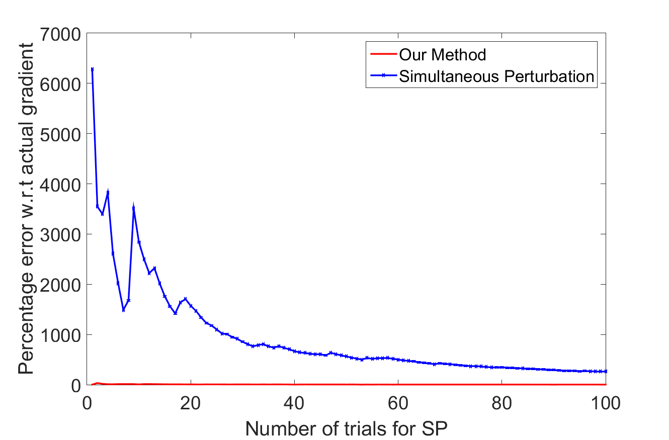
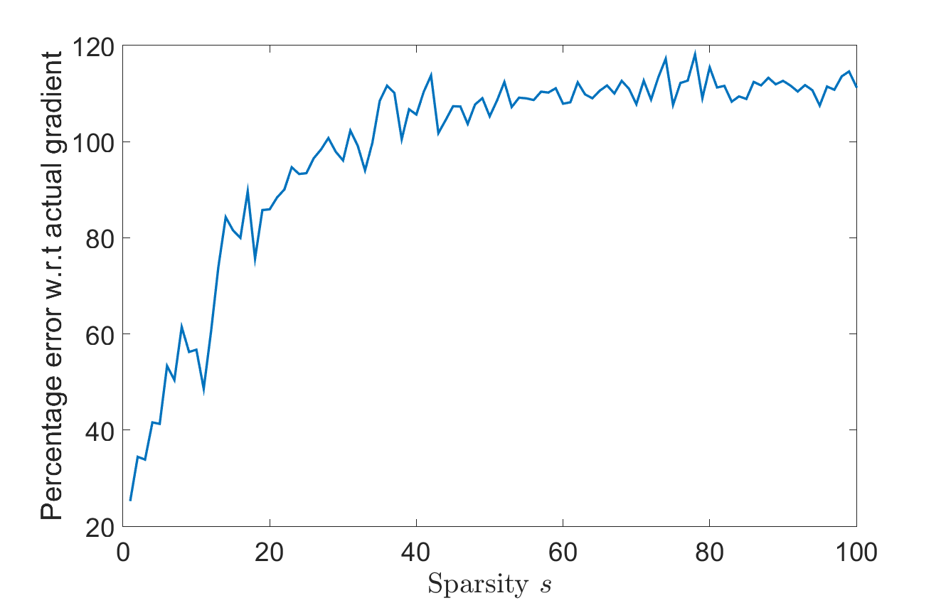
Figures 5 and 5 show that the proposed method works well with higher sparsity levels too. It also shows that with higher , performance of naive SP improves. This is expected. The extremely high error in the naive SP method (especially for small ) is owing to the fact that the actual gradient is extremely sparse and in the beginning SP method ends up populating almost all the coordinates. That contributes to the high percentage of error as seen in the aforementioned figures.
Before we consider specific applications, we illustrate how the percentage error of estimated gradient with varying for different sparsity levels . For appropriately large , for small the error is high (this matches with the discussion in Remark 2). As increases the error is much less. As long as satisfies 2, the compressive sensing results apply. Figure 7 shows the behaviour of the proposed method with variation in the sparsity, but with constant number of observations. We consider -dimensional vector with observations. As expected, for a fixed , as the sparsity increases, increasing no longer helps as the compressive sensing results do not apply and the error increases. was used as a test function for both the simulations.

3.1 Manifold Learning: Estimating e.d.r. space
Consider the following semi-parametric model
where is noise and is a smooth function of the form . Define by the matrix . maps the data to a -dimensional relevant subspace. This means that the function depends on a subspace of smaller dimension given by Range (Note that this is essentially the local view in manifold learning : can vary with location.). The vectors or the directions given by the vectors are called the effective dimension reducing directions or e.d.r. The question is: how to find the matrix ? It turns out that if doesn’t vary in some direction , then where is the gradient outer product matrix defined as
and denotes the expectation over . Lemma 1 from [32] stated below implies that to find the e.d.r. directions it is enough to compute .
Lemma 3.1.
Consider the semi-parametric model
| (12) |
where represents zero mean finite variance noise. Then the espected gradient outer product (EGOP) matrix is of rank at most . Furthermore, if are the eigenvectors associated to the nonzero eigenvalues of , following holds:
Clearly, calculating is computationally heavy. We therefore try to estimate this matrix. Several methods are known for estimating the EGOP and this has been a very popular problem in statistics for a while. The idea of using EGOP for obtaining e.d.r. originated in [20]. While there are other methods based on inverse regression etc., most of the efforts have been directed towards getting an efficient way to estimate gradients in order to finally estimate EGOP (See [33]). In [21], the authors use their method of gradient estimation for this purpose. The idea is to use sample observations for in a neighborhood of the given point and minimize over the error
where are weights (‘kernel’) that favor locality and are typically Gaussian, with regularization in a reproducing kernel Hilbert space (RKHS). The minimizer then is the desired estimate. In [30] a rather simple rough estimator using directional derivative along each coordinate direction is provided. The authors demonstrate that for the purpose of finding e.d.r., a rough estimate such as theirs suffices. We also propose a method via gradient estimation. Take to be the matrix defined by
In other words, , where denotes the estimate of obtained by algorithm 1. We impose our previous restrictions on . That is, the function evaluations at any point are expensive and the gradient of is sparse. In this case we propose an estimate for by the mean of over a sample of points given by the set . By , we shall denote the empirical mean over the sample set . Thus,
and
Theorem 3.2.
The proof closely follows the line of argument in [30].
Proof.
Note that,
The idea is to bound each term. We use concentration inequality for sum of random matrices (See Theorem 2.1, lecture 23 [18] and [31] for more general results) to claim that for ,
with probability . For the second term, it is enough to show that it is bounded for any single sample point . Observe that for any two vectors and , Using this we get, for a fixed ,
| (14) | |||||
with probability , where the last inequality is obtained by applying the bound from Theorem 2.3.
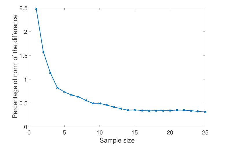
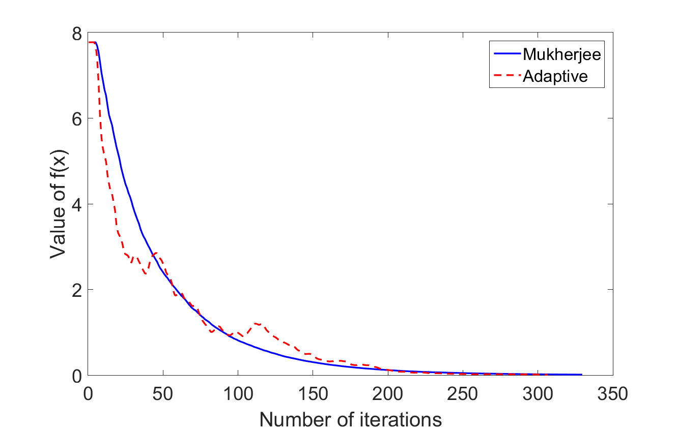
We now simulate an example to illustrate the decay of the error (See Figure 8). Consider a function given by: where, is a -dimensional vector with non-zero elements and corresponds to the dimension of . A Gaussian random matrix is used for the compressive sensing part of the algorithm. The plot of percentage in normed error between and , i.e. is shown below by varying number of samples to . Remember that due to the bias at compressive sensing step, we need to average out the gradient estimation error at SP step. This is done in iterations.
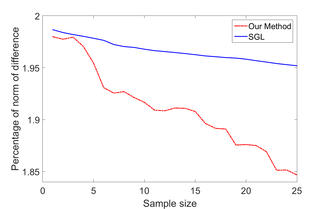
Learning e.d.r. by estimating the gradient using the method proposed in this paper was compared with the SGL (Sparse Gradient Learning) method proposed in [21] using the same function as above and an exponential kernel (See http://www2.stat.duke.edu/~sayan/soft.html for details). Here, and the measurement matrix is a Gaussian matrix. The SP step is averaged over iterations. samples were considered for the SGL method with the neighborhood radius of of . Sparsity of the gradient vector is .
3.2 Optimization
We consider next a typical problem of function minimization, but only consider a function with sparse gradient. In other words, we want to minimize where
is a continuously differentiable real-valued Lipschitz function such that function evaluation at a point in is typically expensive. We also assume that is large and that is sparse. In addition, we assume that the critical points of (i.e., the zeros of ) are isolated. (This is generically true unless there is overparametrization.) The idea is to use the stochastic gradient scheme (3) with the standard assumptions (4), (5). It follows from the theory of stochastic approximation (See [5], Chapter 2) that under above conditions, the solution of the random difference equation (3) tracks with probability one the trajectory of the solution of a limiting o.d.e. as long as the iterates remain bounded, which they do under mild additional conditions on . Following [5], Chapter 2, we use this so called ‘o.d.e. approach’ which states that the algorithm will a.s. converge to the equilibria of the limiting o.d.e., which is
| (15) |
For this, itself serves as the Lyapunov function, leading to the conclusion that the trajectories of (15) and therefore a.s., the iterates of (3) will converge to one of its equilibria, viz., the critical points of . In fact under additional conditions on the noise, it will converge to a (possibly random) stable equilibrium thereof (ibid., Chapter 4).
The stochastic gradient scheme requires at each iteration. The problem, as noted, often is the unavailability of . It is therefore important to have a good method for estimating the gradient. Typically one would obtain noisy measurements and hence the estimate will have a non-zero error . It is known that if the error remains small, the iterates converge a.s. to a small neighbourhood of some point in the set of equilibria of (15). We analyze the resultant error below. Also, the error obtained in SP is zero-mean modulo higher order terms, so one can even take an empirical average over a few separate estimates in order to reduce variance. For high dimensional problems, the number of function evaluations remains still small as compared with, e.g., the classical Kiefer-Wolfowitz scheme. We use Theorem 2.3 to justify using SP (Simultaneous Perturbation Stochastic Approximation) combined with compressed sensing to obtain an approximation for the gradient and then use the above scheme to minimize .
Consider the following stochastic approximation scheme:
| (16) |
where is the additional error arising due to the error in gradient estimation. That is, . If for some small , then the iterates of (16) converge to a small neighbourhood of some point in (See [28] and chapter 10 of [5]). This is ensured by a Lyapunov argument as follows. The limiting o.d.e. is of the form
for some measurable with . Then
which is as long as . Therefore will converge to the set
Assume that the Hessian is positive definite, which is generically so for isolated local minima. Then for small enough, the lowest eigenvalue of for is . By mean value theorem, for some , so . Thus there is convergence to a ball of radius around . (A statement to this result without the estimate on the radius of the ball is contained in Theorem 1 of [14].) Thus we have:
Theorem 3.3.
The stochastic gradient scheme
a.s. converges to a ball of radius centered at some local minimum of , where is the reconstructed gradient as in Theorem 2.3 and is a bound on .
Proof The claim is immediate from the above observations about the perturbed differential equation and Theorem 6, pp. 58-59, [5].
Observe that we have only discussed asymptotic convergence above. For real-life optimization problems, however, we must ensure that the scheme in (16) converges to a neighbourhood of in finite time. This is indeed true and recent concentration-type results (See [19], [29]) strengthen the theoretical basis for plugging in place of in stochastic gradient descent schemes. The results in [19] involve estimates on lock-in probability, i.e., the probability of convergence to a stable equilibrium given that the iterates visit its domain of attraction. An estimate on the number of steps needed to be within a prescribed neighborhood of the desired limit set with a prescribed probability is also obtained. Specifically, the result states that if the th iterate is in the domain of attraction of a stable equilibrium , then after a certain number of additional steps, the iterates remain in a small tube around the differential equation trajectory converging to with probability exceeding
ipso facto implying an analogous claim for the probability of remaining in a small neighborhood of after a certain number of iterates. We refer the reader to [19] for details. In [29], an improvement on this estimate is proved under additional regularity conditions on (twice continuous differentiability) using Alekseev’s formula. We have omitted the details of both the cases as it needs much additional notation to replicate them here. These would, however, apply to the exact stochastic gradient descent. Since we have an additional error due to approximate gradient as in the preceding theorem, we need to combine the results of ibid. with the above theorem to make a weaker claim regarding how small the neighborhood of in question can be. Furthermore, these claims are about iterates which are in the domain of attraction of a stable equilibrium. This, however, is not a problem, as ‘avoidance of traps’ results as in section 4.3 of [5] (see also [3], [4], [24]) ensure that if the noise is rich enough in a certain precise sense, unstable equilibria are avoided with probability one.
Remark 3.
Note that the gradient descent is a stochastic approximation scheme which itself averages out the noise. So in principle the averaging over steps at the SP stage in the original algorithm can be skipped. This means that for a stochastic gradient descent scheme, we cut down the cost of function evaluation even further. The simulations in the next section confirm that good results are obtained without averaging over SP iterations. There is, however, a standard trade-off involved between per step computation / speed of convergence, and fluctuations (equivalently, variance) of the estimates: any additional averaging improves the latter at the expense of the former.
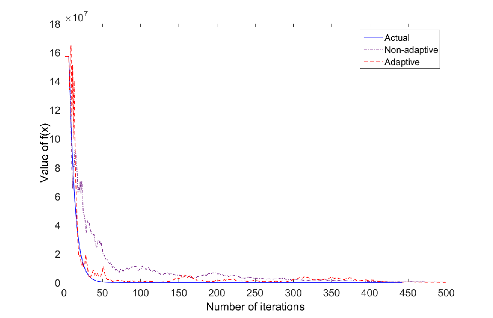
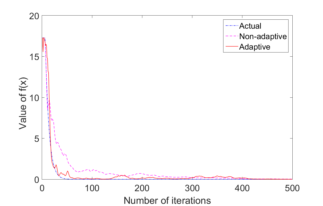
3.3 Numerical experiments
We compare following three algorithms.
-
1.
Actual Gradient Descent
This is the classical stochastic gradient descent with exact gradient.
Algorithm 3 Stochastic Gradient Decent with Compressive Sensing Initialization:
be a sequence that satisfies the properties of stepsize listed above.Iteration: Repeat until convergence criteria is met at . At iteration:
+ errorOutput:
-
2.
Accelerated Gradient Method
Accelerated gradient scheme was proposed by Nesterov [22]. While Gradient Descent algorithm has a rate of convergence of order after steps, Nesterov’s method achieves a rate of order . We implement the method here to achieve an improvement in the time complexity further. The idea is to replace the iteration above by the following.
At iteration:
+ errorwhere, and are as follows:
This gives us faster convergence towards the minimum.
-
3.
Adaptive Method
Another way to achieve a faster convergence rate is to perform the -minimization adaptively with the gradient descent. The idea is to again use the homotopy method for -minimization but this part of the algorithm is run for very few iterations. The intermediate approximation of is then used for performing the stochastic gradient descent. As expected, the errors are high in the beginning but the convergence is faster.
We consider the following function to test our algorithms:
(17) where, function and are random matrices. This is to ensure sparsity of the gradient. Here, and number of non-zero entries in each column of and are . Number of measurements, . is a random Gaussian matrix.
| Algorithm Used | Time taken in Sec for n = 1000 | n = 10000 | n = 25000 |
|---|---|---|---|
| Adaptive Method | 5.910 | 30.4 | 39 |
| With out Adaptive | 50.572 | 213.6 | 489 |
| Actual Gradient Method | 171.150 | 5873.8 | 9000 |
As expected, adaptive method turns out to be faster compared to the non-adaptive method which in turn is much faster than the algorithm that computes actual gradients. Incidentally, the classical scheme all but converges in under 400 iterations. Even so it takes more time than the other two which take more iterations. This is because of the heavy per iterate computation for the classical scheme. From the above table it is clear that as the dimensionality of the problem increases, adaptive method proves more and more useful compared to the other two algorithms.
We compared our method with the method proposed in [21]. The function in (17) is used for the comparison. Here, . Number of samples of SGL were , chosen with neighbourhood radius .
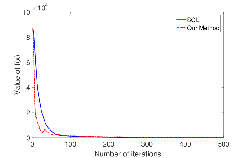
In the following scaled down version and .
The time taken by the SGL method and our method was and seconds respectively. As mentioned earlier, the aim of this paper is to provide a good estimation of gradient when the function evaluations are expensive. In such cases, our method would provide a significant gain in terms of function evaluations needed. While in this example we do see a significant improvement in time taken for the estimation, there is no a priori reason to always expect it. It will indeed be the case when the function evaluations are ‘expensive’ in terms of the time they take. One expects this to be so when the ambient dimension is high.
4 Concluding remarks
We have proposed an estimation scheme for gradient in high dimensions that combines ideas from Spall’s SPSA with compressive sensing and thereby tries to economize on the number of function evaluations. This has theoretical justification by the results of [1]. Our method can be extremely useful when the function evaluation is very expensive, e.g., when a single evaluation is the output of a long simulation. This situation does not seem to have been addressed much in literature. In very high dimensional problems with sparse gradient, computing estimates for partial derivatives in every direction is inefficient because of the large number of function evaluations needed. SP simplifies the problem of repeated function evaluation by concentrating on a single random direction at each step. When the gradient vectors in such cases live in a lower dimensional subspace, it also makes sense to exploit ideas from compressive sensing. We have computed the error bound in this case and have also shown theoretically that this kind of estimation of gradient works well with high probability for the gradient descent problems and in other high dimensional problems such as estimating EGOP in manifold learning where gradients are actually low-dimensional and gradient estimation is relevant. Simulations show that our method works much better than pure SP.
Acknowledgment
We thank GPU Centre of Excellence, IIT Bombay for providing us with the facility to carry out simulations and Prof. Chandra Murthy of Indian Institute of Science for helpful discussions regarding compressive sensing.
References
- [1] T. Austin. On the failure of concentration for the -ball. arXiv preprint arXiv:1309.3315, 2013.
- [2] S. A. Bandeira, M. Fickus, G. D. Mixon, and P. Wong. The road to deterministic matrices with the restricted isometry property. Journal of Fourier Analysis and Applications 19(6): 1123-1149, 2013.
- [3] M. Benaim, A dynamical system approach to stochastic approximation, SIAM Journal of Control and Optimization 34(2): 437-472, 1996.
- [4] O. Brandiére and M. Duflo, Les algorithmes stochastiques contourment - ils les piages?, Annals de l’Institut Henri Poincaré 32(3): 395-427, 1996.
- [5] Vivek S. Borkar. Stochastic Approximation: A Dynamical Systems Viewpoint. Hindustan Book Agency, New Delhi, and Cambridge University Press, Cambridge, UK, 2008.
- [6] E. Candés and T. Tao. Near optimal signal recovery from random projections: universal encoding strategies? IEEE Transactions on Information Theory, 52(12): 5406-5425, 2006.
- [7] E. Candés, J. Romberg J. and T. Tao. Stable signal recovery from incomplete and inaccurate measurements, Comm. Pure Appl. Math., 59(8): 1207-1223, 2006.
- [8] E. Candés, M. Rudelson, T. Tao and R. Vershynin. Error correction via linear programming. In Proceedings of the 46th Annual IEEE Symposium on Foundations of Computer Science (FOCS), pages 295-308, 2005.
- [9] L. W. Chan, K. Charan, D. Takhar, K. F. Kelly, R. G. Baraniuk, G. Richard and D. M. Mittleman. A single-pixel terahertz imaging system based on compressed sensing. Applied Physics Letters, 93(12): 121105-121105-3, 2008.
- [10] M. F. Duarte, M. A. Davenport, T. Dharmpal, J. N. Laska, T. Sun, K. F. Kelly and R. G. Baraniuk. Single-pixel imaging via compressive sampling. IEEE Signal Processing Magazine, 25(2): 83-91, March 2008.
- [11] S. Foucart and H. Rauhut. A Mathematical Introduction to Compressive Sensing, Birkhäuser, New York, 2013.
- [12] A. C. Gilbert, M. J. Strauss, J. A. Tropp and R. Vershynin. One sketch for all: fast algorithms for compressed sensing. Proceedings of the thirty-ninth annual ACM symposium on Theory of computing, 237-246, 2007.
- [13] I. Grondman, L. Busoniu, G. A. D. Lopes and R. Babuska. A Survey of actor-critic reinforcement learning: standard and natural policy gradients. IEEE Transactions on Systems, Man, and Cybernetics, Part C: Applications and Reviews, 42(6): 1291-1307, Nov. 2012.
- [14] M. W. Hirsch. Convergent Activation Dynamics in Continuous Time Networks. Neural Networks, Vol. 2: 331-349, 1989.
- [15] D. R. Jones, M. Schonlau, and W. J. Welch. Efficient global optimization of expensive black box functions. Journal of Global Optimization, 13, 455-492, 1998.
- [16] G. Joseph, C. Murthy. A Non-iterative Online Bayesian Algorithm for the Recovery of Temporally Correlated Sparse Vectors. IEEE Transactions on Signal Processing
- [17] M. Kabanava and H. Rauhut. Analysis -recovery with frames and gaussian measurements. Acta Applicandae Mathematicae, 140(1): 173-195, 2015.
- [18] S. Kakade. Lecture notes on multivariate analysis, dimensionality reduction, and spectral methods. STAT 991, Spring. 2010.
- [19] S. Kamal. ”On the convergence, lock-in probability, and sample complexity of stochastic approximation. SIAM Journal on Control and Optimization, Vol. 48(8): 5178-5192, 2010.
- [20] K. C. Li. Sliced inverse regression for dimension reduction. Journal of the American Statistical Association, 86(414): 316-327, 1991.
- [21] S. Mukherjee, Q. Wu, and D. X. Zhou. Learning gradients on manifolds. Bernoulli, 16(1): 181-207, 2010.
- [22] Y. Nesterov. A method of solving a convex programming problem with convergence rate . Soviet Mathematics Doklady, 27(2): 372-376, 1983.
- [23] P. Pandita, I. Bilionis and J. Panchal. Extending Expected Improvement for High-dimensional Stochastic Optimization of Expensive Black-Box Functions. arXiv preprint arXiv:1604.01147, 2016.
- [24] R. Pemantle, Nonconvergence to unstable points in urn models and stochastic approximation, Annals of Probability 18(2): 698-712, 1990.
- [25] S. Shan, G. Gary Wang. Survey of modeling and optimization strategies to solve high-dimensional design problems with computationally-expensive black-box functions. Structural and Multidisciplinary Optimization, 41(2), 219, 2010.
- [26] J. C. Spall. Multivariate stochastic approximation using a simultaneous perturbation gradient approximation. IEEE Transactions on Automatic Control, 37(3): 332-341, 1992.
- [27] R. S. Sutton, D. McAllester, S. Singh and Y. Mansour. Policy gradient methods for reinforcement learning with function approximation. Advances in Neural Information Processing Systems, 12: 1057-1063, MIT Press, 2000.
- [28] V. B. Tadic and A. Doucet. Asymptotic Bias of Stochastic Gradient Search. 2011 50th IEEE Conference on Decision and Control and European Control Conference (CDC-ECC) Orlando, FL, USA, 2011.
- [29] G. Thoppe and V. S. Borkar. A concentration bound for stochastic approximation via Alexeev’s formula. arXiv:1506-08657v2 [math.OC], 2015.
- [30] S. Trivedi, J. Wang, S. Kpotufe and G. Shakhnarovich. A consistent estimator of the expected gradient outerproduct. Proceedings of the Thirtieth Conference on Uncertainty in Artificial Intelligence: 819-828, July 2014.
- [31] J. A. Tropp. User-friendly tail bounds for sums of random matrices. Foundations of Computational Mathematics, 12(4): 389-434, 2012.
- [32] Q. Wu, J. Guinney, M. Maggioni and S. Mukherjee. Learning gradients : predictive models that infer geometry and statistical dependence. Journal of Machine Learning Research, 11(1922): 2175-2198, 2010.
- [33] Y. Xia, H. Tong, W. Li, and L.-X. Zhu. An adaptive estimation of dimension reduction space. Journal of the Royal Statistical Society: Series B (Statistical Methodology), 64(3): 363-410, 2002.
- [34] H. Xu, C. Caramanis and S. Mannor. Statistical optimization in high dimensions. Operations research, URL = http://dx.doi.org/10.1287/opre.2016.1504, 2016.
- [35] T. Zhao, H. Hachiya, G. Niu and M. Sugiyama. Analysis and improvement of policy gradient estimation. Neural Networks, 26: 118-129, 2012.