Scale invariant behavior in a large N matrix model

Abstract

Eigenvalue distributions of properly regularized Wilson loop operators are used to study the transition from ultra-violet (UV) behavior to infra-red (IR) behavior in gauge theories coupled to matter that potentially have an IR fixed point (FP). We numerically demonstrate emergence of scale invariance in a matrix model that describes $SU(N)$ gauge theory coupled to two flavors of massless adjoint fermions in the large $N$ limit. The eigenvalue distribution of Wilson loops of varying sizes cannot be described by a universal lattice beta-function connecting the UV to the IR.

The Lagrangian of four dimensional gauge theories coupled to massless fermions has no dimensionful parameter. After applying a proper regulator to cure ultra-violet (UV) divergences, the physics in the infra-red (IR) limit is expected to fall into two classes: One provides a quantum description of relativistic particles where the scale invariance of the classical Lagrangian is broken; the second describes a conformal theory with no particle content. QCD, as observed in nature, belongs to the first class. In both classes, the physics at asymptotically short distance scales is described by perturbation theory in terms of a redundant set of local degrees of freedom. The physics at large distances, where the two classes are different, can be easily characterized in terms of non-local observables.

Models in the first class which are “borderline” in terms of their proximity to the second class are central to an activity evaluating certain proposals for beyond the standard model physics Sannino (2009); Lucini (2015). The present work does not consider this issue. For us, the mere existence of an interacting conformal gauge theory in four dimensions which seems to require no fine tuning on the lattice to boot, makes the study of class two models deserving of attention on its own.

Let $a$ denote an UV regulator with dimensions of length and let $g$ be the bare coupling introduced into the Lagrangian. This enables one to perform a calculation that produces a finite result at a fixed $a$ and $g$. We define a dimensionless physical coupling, $g_{R}(\ell;a,g)$, that depends on the physical scale $\ell$ and obeys a Renormalization Group (RG) equation:

$$\left[a\frac{\partial}{\partial a}+\beta(g)\frac{\partial}{\partial g}\right]g_{R}(\ell;a,g)=0;\ \ \ \ \ \beta(0)=0;$$ (1)

for every choice of $\ell$. The content of the equation is that $g$ depends on $a$ via

$$\frac{dg}{d\ln a}+\beta(g)=0;$$ (2)

and we can write our observable as $g_{R}(\ell;g(a))$. Noting that

$$\left[\frac{\partial}{\partial\ln\ell}+\frac{\partial}{\partial\ln a}\right]g_{R}(\ell;g(a))=0,$$ (3)

we change variable from $g$ to $g_{R}(\ell;g(a))$ for a fixed $\ell$ and obtain the renormalized version of Eq. (2) as

$$\frac{\partial g_{R}(\ell)}{\partial\ln\ell}=\beta_{R}(g_{R}(\ell));\ \ \ \ \ \beta_{R}(0)=0;$$ (4)

where the reference to the the UV regulator, $a$, naturally drops out. In perturbation theory, the first two coefficients in the expansion of the renormalized beta function,

$$\beta_{R}(g_{R}(\ell))=\beta_{0}g_{R}^{3}(\ell)+\beta_{1}g_{R}^{5}(\ell)+\cdots,$$ (5)

are the same as that of the unrenormalized beta function $\beta(g)$. It is tempting to define a new renormalized coupling where the associated beta function is exactly given by the first two terms in Eq. (5). This new renormalized coupling will admit a Taylor expansion in terms of the old coupling around the joint value 0. There is no guarantee that this new renormalized coupling and the bare coupling $g$ are related by a map that is well behaved at all points away from the origin.

If we assume that $\beta_{R}(g_{R}(\ell))$ remains positive for all $\ell>0$, it follows from the RG equation for $g_{R}(\ell)$ that it grows monotonically without bound as $\ell$ increases, starting from $g_{R}(0_{+})=0_{+}$ . There is only one length scale in such a theory: A scale, $\ell_{0}$, beyond which higher order terms in Eq. (5) begin to matter and the theory becomes non-perturbative. In a theory like QCD, $\ell_{0}$ is close to 1 fermi  and long distance physics can be numerically studied with small systematic errors by simulating QCD in a periodic box with a linear extent of few fermi.

Now consider theories where $\beta_{R}(g^{*})=0$ and becomes negative for $g_{R}>g^{*}>0$. The renormalization coupling constant will not grow without bound; instead, it will start from $g_{R}(0_{+})=0_{+}$ and reach $g_{R}(\infty)=g^{*}$. In such a theory, we expect that two physically relevant length scales $\ell_{s}\ll\ell_{l}$ exist, such that $g_{R}(\ell)$ will be governed by perturbation theory for $\ell<\ell_{s}$ and become scale invariant for $\ell>\ell_{l}$. In order to see the onset of scale invariance, a numerical study should be performed in a periodic box with a linear extent significantly larger than $\ell_{l}$ and this will be practically impossible if also $\ell_{s}\ll\ell_{l}$ holds. Two scale problems are notoriously difficult to control by numerical methods. They are also a challenge to analytical methods.

We will consider $SU(N)$ gauge theory with $n_{M}$ flavors of massless Majorana fermions in the adjoint representation in this paper. For this theory Caswell (1974),

$$\beta_{0}=\frac{N\left(11-2n_{M}\right)}{48\pi^{2}};\ \ \ \ \ \beta_{1}=\frac{N^{2}\left(17-8n_{M}\right)}{384\pi^{4}}.$$ (6)

If $\frac{17}{8}<n_{M}<\frac{11}{2}$, we have $\beta_{0}>0$ and $\beta_{1}<0$ and

$$\frac{5}{7}\geq\frac{{g^{*}_{2}}^{2}N}{8\pi^{2}}\geq\frac{1}{23}\ \ \ \ \ {\rm for}\ \ \ 3\leq n_{M}\leq 5,$$ (7)

as given by the first two terms in Eq. (5). It is unlikely, this estimate of $g^{*}$ is correct even for $n_{M}=5$.

The lattice action for massless fermions coupled to gauge fields has one coupling, $b=1/\lambda$, where $\lambda=g^{2}N$ is the ’t Hooft coupling. The aim of a lattice study of a theory that possibly exhibits scale invariance in the IR is not necessarily to identify a RG trajectory along which to carry out simulations, since a trajectory connecting $\ell_{s}$ to $\ell_{l}$ might require a path visiting actions containing a large number of terms with many couplings that need to be precomputed. Keeping only one coupling $b$, all we can say with some certainty is that at large $b$ its variation is tangential to this RG trajectory. Once the regime of large $b$ is left we likely wander off quite far from any RG trajectory corresponding to some decent RG transformation. A “decent” RG trajectory is defined by a RG transformation in the space of actions which respects all important symmetries and is local, in the sense that the new fields are local functionals of the old fields. Also, it is required to check that the space of couplings one needs to keep track of is of a low dimension to good numerical accuracy (that is most of the couplings of the infinite space of actions can be ignored).

The continuum situation may be taken to simply indicate that for more or less all $b$’s the single coupling system is critical, and its large distance asymptotic behavior is scale and conformal invariant. We don’t ever sit at, or are close to, the IR fixed point of some RG map: only the large distance behavior is governed by some IR FP. This is the generic case for a critical system. For a given $b$ there will two scales, $L_{s}(b)<<L_{l}(b)$ in lattice units. For $L<L_{s}(b)$ scaling is violated as in QCD and for $L>L_{l}(b)$ scaling is restored but the dimensions take “anomalous” values. As we vary $b$ in some range, $b\in(b_{0},b_{\infty})$, the $L_{s}(b)<<L_{l}(b)$ vary, but outside this range their very definitions are in jeopardy and may become inconsistent. For intermediate scales $L$, $L_{s}(b)<L<L_{l}(b)$, the most plausible behavior is one strongly dependent on the form of the lattice action. There, lattice observables cannot be described by a continuum action on some RG trajectory. In short, the UV - IR interpolation offered by a single coupling lattice action does not necessarily admit a useful continuum description throughout, but only at sufficiently short and sufficiently long scales.

Large $N$ reduction enables one to reduce the lattice action to a matrix model Eguchi and Kawai (1982); Gonzalez-Arroyo and Okawa (1983). In some cases, the matrix model reproduces physics at infinite volume lattice theory. For QCD-like theories with the number of Dirac flavors in the fundamental representation kept finite this connection breaks down as one approaches the continuum limit $b\to\infty$ Bhanot et al. (1982). This breakdown can be avoided if one uses more than a modest amount of adjoint matter Mkrtchyan and Khokhlachev (1983); Kovtun et al. (2007); Hietanen and Narayanan (2010). Assuming no other problems with large $N$ reduction, this offers the opportunity to look for asymptotic scale invariance in a large $N$ matrix model.

We will require non-local observables to properly study the IR behavior. A basic set of non-local operators in the continuum or on the lattice is given by Wilson Loops (WL). We proceed using continuum language. Classically, for $SU(N)$, these are unitary matrices associated with closed smooth spacetime curves $\mathcal{C}$. Quantum mechanically one needs to renormalize, giving the loop an effective thickness:

$$W_{f}(\mathcal{C},x,s)=\mathcal{P}\exp\left(i\oint^{x}_{x;\mathcal{C}}A^{f}_{\mu}(y,s)dy_{\mu}\right)\in SU(N)$$ (8)

$f$ denotes the fundamental representation of $SU(N)$ and $x$ is a marked point on $\mathcal{C}$. $s$ is a smearing parameter, providing the thickness. The $N\times N$ matrix $W_{f}$ has operator valued entries which obey $[W_{f}W_{f}^{\dagger}]_{ij}=\delta_{ij}\mathbb{I},\;\det(W_{f})=\mathbb{I}$.

Starting from the four dimensional quantum field, $B^{f}_{\mu}(x)$; $x\in R^{4}$, appearing in the path integral, the act of smearing Narayanan and Neuberger (2006); Lohmayer and Neuberger (2011) extends the gauge fields to the five dimesional space, $R^{4}\times R_{+}$, with the smearing parameter $s\in R_{+}$. The five dimensional gauge fields, $A^{f}_{\mu}(x,s)$ are defined for $s\geq 0$ by

$$F_{\mu s}=D_{\nu}F_{\mu\nu};~{}~{}~{}~{}~{}~{}~{}~{}~{}~{}~{}~{}~{}{A^{f}_{\mu}(x,s=0)=B^{f}_{\mu}(x)}.$$ (9)

Note that $s$ has dimensions of area. The 5D gauge freedom is partially fixed, leaving a 4D one, by $A^{f}_{s}(x,s)=0$. All divergences coming from coinciding spacetime points in products of renormalized elementary fields are eliminated for $s>0$ by a limitation on the resolution of the observer, parametrized by $s$. In QCD, a reasonable value for $s$ for a loop of size $\sim 1\;\text{fermi}$ is $s\sim 0.05\ \text{fermi}^{2}$.

Let us focus on square Wilson loops of side $\ell$, noting that the effects of the sharp corners have also been smoothed out by the smearing. For every such $W_{f}(\ell,x,s)$ we consider its set of eigenvalues

$$\Theta(\ell,s)=\{e^{i\theta_{1}},...,e^{i\theta_{N}}\},\ \ \ \ \ \sum_{i=1}^{N}\theta_{i}=0\mod 2\pi.$$ (10)

The label $x$ drops out since the eigenvalues do not depend on the choice of the point $x$ on $\mathcal{C}$. $\Theta(\ell,s)$ parametrizes the gauge invariant content of $W_{f}(\ell,x,s)$. Using the eigenvalues, $\Theta(\ell,s)$, we can define vacuum averages which provide the complete information about the $\Theta(\ell,s)$ in terms of $n$-angle densities $p(\Theta;\ell,s)$ normalized to unity. $p$ contains a periodic $\delta$-function representing the $\det=1$ constraint. Instead of working with two dimensional parameters $(\ell,s)$ we change the variables to $(\ell,f=\frac{s}{\ell^{2}})$. We focus on the simplest marginal of $p$, the normalized single-angle eigenvalue distribution

$$\rho(\theta,f;\ell)=\frac{1}{N}\sum_{i=1}^{N}\left[\prod_{j=1}^{N}\int_{0}^{2\pi}d\theta_{j}\right]p(\Theta,s=f\ell^{2};\ell)\delta(\theta-\theta_{i});\ \ \ \ \int_{0}^{2\pi}d\theta\rho(\theta;\ell,f)=1.$$ (11)

$\rho$ carries no information about correlations between the various $\theta_{i}$. The question of interest is how the dimensionless $\rho(\theta,f;\ell)$ depends on $\ell$ for a fixed $f$.

In the case of pure gauge theory, $\rho(\theta,f;l)$ provides an acceptable definition of a $\theta$ independent $\beta$-function because the $\theta$-dependence admits an accurate parametrization by one variable only. The observable, $\rho(\theta,f;\ell)$, has proved to be quite useful in understanding the transition from weak coupling to strong coupling in the large $N$ limit of QCD Narayanan and Neuberger (2006, 2007); Lohmayer and Neuberger (2012). In the ’t Hooft $N=\infty$ limit oscillations in $\theta$ disappear from $\rho(\theta,f;\ell)$ and $\rho$ is very smooth almost everywhere, but a non-analyticity in the dependence on $\ell$ appears at some $\ell_{c}$. For $\ell<\ell_{c}$ the support of $\rho(\theta,f;\ell)$ is restricted to an arc $<2\pi$ symmetrically around $\theta=0$. For $\ell>\ell_{c}$ the support is the entire unit circle. For any finite $N>>1$ the transition is smoothed out. For $N>>1$ the $\ell$-dependence for $\ell\approx\ell_{c}$ is universal. If one uses a related observable, the average of the characteristic polynomial of the WL, a derived quantity from it is very well described by Burgers’ equation with viscosity $\frac{1}{2N}$ Neuberger (2008).

Because perturbation theory amounts to path-integral integration over the Lie algebra $su(N)$ and not over the group $SU(N)$ the large $N$ transition at $\ell_{c}$ demarcates a scale where the prediction from perturbation theory depart substantially from the true values. That there exists an $\ell_{c}$ Blaizot and Nowak (2008) does not imply confinement, only removes an obstacle to it at $\ell>\ell_{c}$, by closing the gap in the eigenvalue distribution. Confinement is reflected by the eigenvalue distribution approaching uniformity exponentially in $\ell^{2}$ as $\ell\to\infty$. This behavior occurs far from $\ell_{c}$ and has nothing to do with the mechanism that produced $\ell_{c}$ in the first place.

Consider a theory that is expected to be scale invariant in the IR. Let us consider the lattice version of single-angle eigenvalue distribution, $\rho(\theta,f;b,L)$, where $L$ is the linear extent of the loop in lattice units. If $L<L_{s}(b)$, we will find a strong dependence of the distribution on $b$ and $L$ separately. But, we will be able to absorb it by finding a function $L(b)$ such that the distribution only depends on $L(b)$. The resulting continuum distribution will exhibit the UV nature of the theory.

If $L>L_{l}(b)$, we should expect the distribution to stabilize and essentially become independent of $L$ and $b$. The resulting stable continuum distribution exhibits the scale invariance in the IR. The distribution in the cross-over region, $L_{s}(b)<L<L_{l}(b)$ will show dependence on $L$ and $b$. If we define a lattice $\beta$-function with argument $\lambda=1/b$ in the crossover range by $[L\frac{\partial}{\partial L}-\beta(\lambda)\frac{\partial}{\partial\lambda}]\rho(\theta;\lambda,L)=0$ we shall find that $\beta(\lambda)$ comes out strongly $\theta$ dependent and is therefore not universal in any sense. These $\beta(\lambda)$ functions have lost all the power that the $\beta(\lambda)$ functions have at short distances, where they are universal.

A natural way to single out theories exhibiting “perturbative IR behavior” is to require that the lattice $\rho(\theta;L)$ have a gapped contiguous support on the unit circle $\forall L$, including at $L\to\infty$. This definition is at $N=\infty$. If we have “perturbative IR behavior” there is reason to hope that a simple single coupling lattice approximation to the continuum RG trajectory holds.

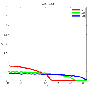
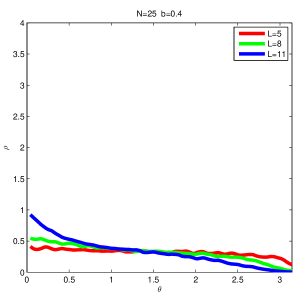
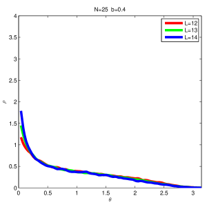
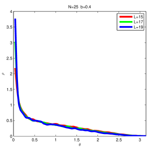
Figure 1: The distributions, $\rho(\theta,f;b,L)$, are shown for several different values of $L$ at $b=0.4$. The value of $N$ is $25$ and the value of $f$ is set to $10^{-3}$. The value of $L$ increases as one goes from top-left to bottom-right with different panels showing different regions of $L$.

We will now provide numerical results for $\rho(\theta,f;b,L)$ in a matrix model where the IR behavior is not expected to be perturbative. The model is a single site SU(N) gauge theory coupled to two massless Majorana fermions realized using overlap fermions Hietanen and Narayanan (2012). We will provide results for $N=25$ which we consider to be large in the sense that the large $N$ limit for this particular lattice model is reasonably well approximated for most of the observables we look at. We will show data for three different values of lattice coupling, $b=0.4,0.5,0.6$. The lattice version of Eq. (9) is realized as follows: Let $U_{\mu}(s)=e^{iA_{\mu}(s)}$ be the four smeared link variables on the single site lattice. The smeared plaquettes are given by

$$P_{\mu\nu}(s)=U_{\mu}(s)U_{\nu}(s)U_{\mu}^{\dagger}(s)U_{\nu}^{\dagger}(s).$$ (12)

Then,

$$D_{\nu}F_{\mu\nu}(s)=i\sum_{\nu}\left[P_{\mu\nu}^{\dagger}(s)+U_{\nu}^{\dagger}(s)P_{\mu\nu}(s)U_{\nu}(s)-P_{\mu\nu}(s)-U_{\nu}^{\dagger}(s)P_{\mu\nu}^{\dagger}(s)U_{\nu}(s)\right].$$ (13)

The evolution of $U_{\mu}(s)$ as per Eq. (9) becomes

$$\frac{dU_{\mu}(s)}{ds}=-iD_{\nu}F_{\mu\nu}(s)U_{\mu}(s).$$ (14)

The folded and smeared Wilson loops used in the computation of $\rho(\theta,f;b,L)$ are

$$W_{\mu\nu}(L,s=fL^{2})=\left[U_{\mu}(s)\right]^{L}\left[U_{\nu}(s)\right]^{L}\left[U_{\mu}^{\dagger}(s)\right]^{L}\left[U_{\nu}^{\dagger}(s)\right]^{L}.$$ (15)

Figure 1 shows the results for $\rho(\theta,f;b,L)$ for different values of $L$ at $b=0.4$ and $f=10^{-3}$. The top-left panel shows the behavior for $L<L_{s}(b)$. The $L=1$ and $L=2$ distributions show a gap with a larger gap for $L=1$. The $L=3$ distribution is gap-less. The top-right panel shows the transition of $L$ into the region, $L_{s}(b)<L<L_{l}(b)$. The distributions still remain gap-less but increasing $L$ results in a distribution that is more peaked around $\theta=0$. The bottom-left panel shows the development of scale invariant distribution as $L$ moves closer to $L_{l}(b)$. The bottom-right panel shows distributions for $L>L_{l}(b)$ that are essentially scale invariant. The distributions show a fast rise around $\theta=0$ but have stabilized away from $\theta=0$. This could be indicative of a limiting distribution that has an integrable singularity at $\theta=0$. Figure 2 shows the distribution as a function of $b$ for $L=19$ which is above $L_{l}(b)$ for all three values of $b$. A scale invariant distribution seems to have emerged.

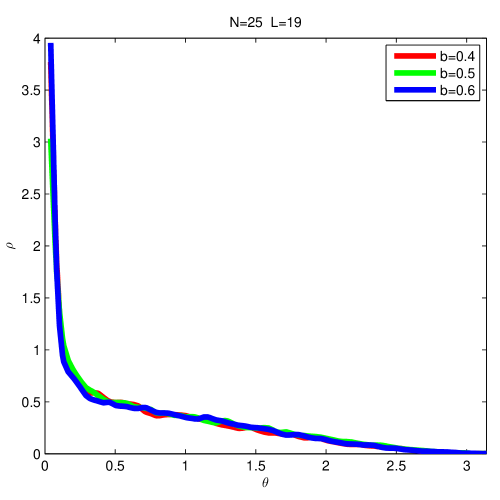
Figure 2: The distributions, $\rho(\theta,f;b,L)$, are shown for $b=0.4,0.5,0.6$ at $L=19$. The value of $N$ is $25$ and the value of $f$ is set to $10^{-3}$.

We have demonstrated that scale invariance can emerge in a matrix model, indicating the existence of an IR FP. The scales $L_{s}(b)$ and $L_{l}(b)$ have a ratio of order $5$ and the set of lattice model for all couplings is far from making up an acceptable RG trajectory at intermediary scales. The scale invariant angle distribution is gap-less. Therefore there is no indication for a concrete perturbative lattice realization of an IR FP. We have demonstrated that $\rho(\theta,f;b,L)$ is a useful probe of the theory. This probe can be defined, and we suggest it will be useful, also at finite $N$.

This eigenvalue distribution reflects relatively simple physics for adjoint matter models: the force between fundamental test charges at distance $r$ is stronger than a Coulomb $1/r^{2}$ at short distances, raises to some constant value as $r$ increases further, but eventually turns around and goes like ${\rm Const}/r^{2}$ as $r\to\infty$. For a perturbative IR FP, the intermediary constant force regime would have to be skipped. A priori, there seems to be nothing prohibiting this from occurring, but this did not happen in our model.

The matrix model of Hietanen and Narayanan (2012) has the Wilson mass parameter that appears in the massless overlap fermion kernel set to $4$ in order to ensure proper reduction. In the present work we have re-analyzed data generated for  Hietanen and Narayanan (2012) for lattice gauge couplings $b$ in the range $[0.32,0.70]$. Already in Hietanen and Narayanan (2012) lattice beta functions were found to be far away from two loop perturbation theory for this range of couplings.

We plan to continue our work with more extensive numerical studies on the lines of the present paper, using the results of  Lohmayer and Narayanan (2013) and ensuring that the center symmetries remain intact. The formulation adopted here allows us to extend the matrix model to nonintergal numbers of massless flavors, a device that can, at the formal level, reduce the contribution of higher than two-loop terms to perturbative beta-functions at will. Also, it would increase our confidence in the relevance of the matrix model to the full lattice theory if we could increase $N$ relative to the $L$ values we now know we need. Recent interesting work on reduced model manages to deal with substantially larger values of $N$ García Pérez et al. (2015). This work uses also the device of twisted reduction. For an amount of matter $n_{M}\geq 1$ twisting, or any other trick on top of original Eguchi-Kawai reduction is not perturbatively required. Dropping twisting would simplify numerical work and might reduce the cost of simulations at $N$ of order 100 to something manageable on modest PC clusters.