Phase Transitions in Semidefinite Relaxations

Abstract

Statistical inference problems arising within signal processing, data mining, and machine learning naturally give rise to hard combinatorial optimization problems. These problems become intractable when the dimensionality of the data is large, as is often the case for modern datasets. A popular idea is to construct convex relaxations of these combinatorial problems, which can be solved efficiently for large scale datasets.

Semidefinite programming (SDP) relaxations are among the most powerful methods in this family, and are surprisingly well-suited for a broad range of problems where data take the form of matrices or graphs. It has been observed several times that, when the ‘statistical noise’ is small enough, SDP relaxations correctly detect the underlying combinatorial structures.

In this paper we develop asymptotic predictions for several ‘detection thresholds,’ as well as for the estimation error above these thresholds. We study some classical SDP relaxations for statistical problems motivated by graph synchronization and community detection in networks. We map these optimization problems to statistical mechanics models with vector spins, and use non-rigorous techniques from statistical mechanics to characterize the corresponding phase transitions. Our results clarify the effectiveness of SDP relaxations in solving high-dimensional statistical problems.

1 Introduction

Many information processing tasks can be formulated as optimization problems. This idea has been central to data analysis and statistics at least since Gauss and Legendre’s invention of the least-squares method in the early 19th century [Gau09].

Modern datasets pose new challenges to this centuries’ old framework. On the one hand, high-dimensional applications require to estimate simultaneously millions of parameters. Examples span genomics [BDSY99], imaging [P⁺09], web-services [KBV09], and so on. On the other hand, the unknown object to be estimated has often a combinatorial structure: In clustering we aim at estimating a partition of the data points [VL07]. Network analysis tasks usually require to identify a discrete subset of nodes in a graph [GN02, KMM⁺13]. Parsimonious data explanations are sought by imposing combinatorial sparsity constraints [Was00].

There is an obvious tension between the above requirements. While efficient algorithms are needed to estimate a large number of parameters, the maximum likelihood method often requires to solve NP-hard combinatorial optimizations. A flourishing line of work addresses this conundrum by designing effective convex relaxations of these combinatorial problems [Tib96, CDS98, CT10].

Unfortunately, the statistical properties of such convex relaxations are well understood only in a few cases (compressed sensing being the most important success story [DT05, CT07, DMM09, ALMT14]). In this paper we use tools from statistical mechanics to develop a precise picture of the behavior of a class of semidefinite programming relaxations. Relaxations of this type appear to be surprisingly effective in a variety of problems ranging from clustering to graph synchronization. For the sake of concreteness we will focus on three specific problems:

${\mathbb{Z}}_{2}$-synchronization. In the general synchronization problem, we aim at estimating $x_{0,1},x_{0,2},\dots,x_{0,n}$ which are unknown elements of a known group ${\mathfrak{G}}$. This is done using data that consists of noisy observations of ‘relative positions’ $Y_{ij}=x_{0,i}^{-1}x_{0,j}+{\sf noise}$. A large number of practical problems can be modeled in this framework. For instance, the case ${\mathfrak{G}}=SO(3)$ (the orthogonal group in three dimensions) is relevant for camera registration, and molecule structure reconstruction in electron microscopy [SS11].

The ${\mathbb{Z}}_{2}$-synchronization problem is arguably the simplest problem in this class, and corresponds to ${\mathfrak{G}}={\mathbb{Z}}_{2}$ (the group of integers modulo $2$). Without loss of generality, we will identify this with the group $(\{+1,-1\},\,\cdot\,)$ (elements of the group are $+1$, $-1$ and the group operation is ordinary multiplication). We assume observations to be distorted by Gaussian noise, namely for each $i<j$ we observe $Y_{ij}=(\lambda/n)\,x_{0,i}x_{0,j}+W_{ij}$, where $W_{ij}\sim{\sf N}(0,1/n)$ are independent standard normal random variables. This fits the general definition since $x_{0,i}^{-1}=x_{0,i}$ for $x_{0,i}\in\{+1,-1\}$.

In matrix notation, we observe a symmetric matrix $\bm{Y}=\bm{Y}^{*}\in{\mathbb{R}}^{n\times n}$ given by

$$\bm{Y}=\frac{\lambda}{n}\,\bm{x_{0}}\,\bm{x_{0}}^{*}+\bm{W}\,.$$ (1)

(Note that entries on the diagonal carry no information.) Here $\bm{x_{0}}\in\{+1,-1\}^{n}$, $\bm{x_{0}}^{*}$ denote the transpose of $\bm{x_{0}}$, and $\bm{W}=(W_{ij})_{i,j\leq n}$ is a random matrix from the Gaussian Orthogonal Ensemble (GOE), i.e. a symmetric matrix with independent entries (up to symmetry) $(W_{ij})_{1\leq i<j\leq n}\sim_{i.i.d.}{\sf N}(0,1/n)$ and $(W_{ii})_{1\leq i\leq n}\sim_{i.i.d.}{\sf N}(0,2/n)$.

A solution of the ${\mathbb{Z}}_{2}$ synchronization problem can be interpreted as a bi-partition of the set $\{1,\dots,n\}$, and hence this has been used as a model for partitioning signed networks [Cuc15, ABBS14].

$U(1)$-synchronization. This is again an instance of the synchronization problem. However, we take ${\mathfrak{G}}=U(1)$. This is the group of complex number of modulus one, with the operation of complex multiplication ${\mathfrak{G}}=(\{x\in{\mathbb{C}}:\,|x|=1\},\,\cdot\,)$

As in the previous case, we assume observations to be distorted by Gaussian noise, i.e. for each $i<j$ we observe $Y_{ij}=(\lambda/n)\,x_{0,i}\overline{x}_{0,j}+W_{ij}$, where $\overline{z}$ denotes complex conjugation and $W_{ij}\sim{\sf CN}(0,1/n)$.

In matrix notations, this model takes the same form (1), provided we interpret $\bm{x_{0}}^{*}$ as the conjugate transpose of vector $\bm{x_{0}}\in{\mathbb{C}}^{n}$, with components $x_{0,i}$, $|x_{0,i}|=1$. We will follows this convention throughout.

$U(1)$ synchronization has been used as a model for clocks synchronization over networks [Sin11, BBS14]. It is also closely related to the phase-retrieval problem in signal processing [CESV15, WdM15, ABFM14]. An important qualitative difference with respect to the previous example (${\mathbb{Z}}_{2}$ synchronization) lies in the fact that $U(1)$ is a continuous group. We regard this as a prototype of synchronization problems over compact Lie groups (e.g. $SO(3)$)

Hidden partition (a.k.a. community detection). The hidden (or planted) partition model is a statistical model for the problem of finding clusters in large network datasets (see [KMM⁺13, Mas14, MNS13] and references therein for earlier work). The data consist of graph $G=(V,E)$ over vertex set $V=[n]\equiv\{1,2,\dots,n\}$ generated as follows. We partition $V=V_{+}\cup V_{-}$ by setting $i\in V_{+}$ or $i\in V_{-}$ independently across vertices with ${\mathbb{P}}(i\in V_{+})={\mathbb{P}}(i\in V_{-})=1/2$. Conditional on the partition, edges are independent with

$${\mathbb{P}}\big{\{}(i,j)\in E\,\big{|}\,V_{+},V_{-}\big{\}}=\begin{cases}a/n&\mbox{ if $\{i,j\}\subseteq V_{+}$ or $\{i,j\}\subseteq V_{-}$,}\\ b/n&\mbox{ otherwise.}\\ \end{cases}$$ (2)

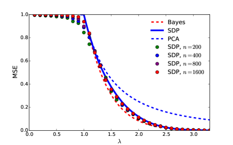
Figure 1: Estimating $\bm{x_{0}}\in\{+1,-1\}^{n}$ under the noisy ${\mathbb{Z}}_{2}$ synchronization model of (1). Curves correspond to (asymptotic) analytical predictions, and dots to numerical simulations (averaged over $100$ realizations).

Here $a>b>0$ are model parameters that will be kept of order one as $n\to\infty$. This corresponds to a random graph with bounded average degree $d=(a+b)/2$, and a cluster (a.k.a. ‘block’ or ‘community’) structure corresponding to the partition $V_{+}\cup V_{-}$. Given a realization of such a graph, we are interested in estimating the underlying partition.

We can encode the partition $V_{+}$, $V_{-}$ by a vector $\bm{x_{0}}\in\{+1,-1\}^{n}$, letting $x_{0,i}=+1$ if $i\in V_{+}$ and $x_{0,i}=-1$ if $i\in V_{-}$. An important insight –that we will develop below– is that this problem is analogous to ${\mathbb{Z}}_{2}$-synchronization, with signal strength $\lambda=(a-b)/\sqrt{2(a+b)}$. The parameters’ correspondence is obtained, at a heuristics level, by noting that, if $\bm{A}_{G}$ is the adjacency matrix of $G$, then ${\mathbb{E}}\langle\bm{x_{0}},\bm{A}_{G}\bm{x_{0}}\rangle/(n{\mathbb{E}}\|\bm{A}_{G}\|^{2}_{F})^{1/2}\approx(a-b)/\sqrt{2(a+b)}$. (Here and below $\langle{\bm{a}},{\bm{b}}\rangle=\sum_{i}a_{i}b_{i}$ denotes the standard scalar product between vectors.)

A generalization of this problem to the case of more than two blocks has been studied since the eighties as a model for social network structure [HLL83], under the name of ‘stochastic block model.’ For the sake of simplicity, we will focus here on the two-blocks case.

2 Illustrations

As a first preview of our results, Figure 1 reports our analytical predictions for the estimation error in the ${\mathbb{Z}}_{2}$ synchronization problem, comparing them with numerical simulations using SDP. An estimator is a map $\bm{\hat{x}}:{\mathbb{R}}^{n\times n}\to{\mathbb{R}}^{n}$, $\bm{Y}\mapsto\bm{\hat{x}}(\bm{Y})$. We compare various estimators in terms of their per-coordinate mean square error:

$${\rm MSE}_{n}(\bm{\hat{x}})\equiv\frac{1}{n}{\mathbb{E}}\big{\{}\min_{s\in\{+1,-1\}}\|\bm{\hat{x}}(\bm{Y})-s\,\bm{x_{0}}\big{\|}_{2}^{2}\big{\}}\,,$$ (3)

where expectation is with respect to the noise model (1) and $\bm{x_{0}}\in\{+1,-1\}^{n}$ uniformly random. Note the minimization with respect to the sign $s\in\{+1,-1\}$ inside the expectation: because of the symmetry of (1), the vector $\bm{x_{0}}$ can only be estimated up to a global sign. We will be interested in the high-dimensional limit $n\to\infty$ and will omit the subscript $n$ –thus writing ${\rm MSE}(\bm{\hat{x}})$– to denote this limit. Note that trivial estimator that always returns $0$ has error ${\rm MSE}_{n}({\mathbf{0}})=1$, and hence for every other method we should achieve ${\rm MSE}(\bm{\hat{x}})\in[0,1]$,

Classical statistical theory suggests two natural reference estimators: the Bayes-optimal and the maximum likelihood estimators. We will discuss these methods first, in order to set the stage for SDP relaxations.

Bayes-optimal estimator (a.k.a. minimum MSE). This provides a lower bound on the performance of any other approach. It takes the conditional expectation of the unknown signal given the observations:

$$\bm{\hat{x}}^{\mbox{\tiny{Bayes}}}(\bm{Y})={\mathbb{E}}\big{\{}\,{\bm{x}}\,\big{|}\,(\lambda/n){\bm{x}}{\bm{x}}^{*}+\bm{W}=\bm{Y}\big{\}}\,.$$ (4)

Explicit formulas are given in Supplementary Information (SI). We note that $\bm{\hat{x}}^{\mbox{\tiny{Bayes}}}(\bm{Y})$ assumes knowledge of the prior distribution. The red-dashed curve in Fig. 1 presents our analytical prediction for the asymptotic MSE for $\bm{\hat{x}}^{\mbox{\tiny{Bayes}}}(\,\cdot\,)$. Notice that ${\rm MSE}(\bm{\hat{x}}^{\mbox{\tiny{Bayes}}})=1$ for all $\lambda\leq 1$ and ${\rm MSE}(\bm{\hat{x}}^{\mbox{\tiny{Bayes}}})<1$ strictly for all $\lambda>1$, with ${\rm MSE}(\bm{\hat{x}}^{\mbox{\tiny{Bayes}}})\to 0$ quickly as $\lambda\to\infty$. The point $\lambda_{c}^{\mbox{\tiny{Bayes}}}=1$ corresponds to a phase transition for optimal estimation, and no method can have non-trivial ${\rm MSE}$ for $\lambda\leq\lambda_{c}^{\mbox{\tiny{Bayes}}}$.

Maximum likelihood (MLE). The estimator $\bm{\hat{x}}^{\mbox{\tiny{ML}}}(Y)$ is given by the solution of

$$\bm{\hat{x}}^{\mbox{\tiny{ML}}}(\bm{Y})=c(\lambda)\,{\arg\!\max}_{{\bm{x}}\in\{+1,-1\}^{n}}\;\langle{\bm{x}},\bm{Y}{\bm{x}}\rangle\;\,.$$ (5)

Here $c(\lambda)$ is a scaling factor that is chosen according to the asymptotic theory as to minimize the MSE. As for the Bayes-optimal curve, we obtain ${\rm MSE}(\bm{\hat{x}}^{\mbox{\tiny{ML}}})=1$ for $\lambda\leq\lambda_{c}^{\mbox{\tiny{ML}}}=1$ and ${\rm MSE}(\bm{\hat{x}}^{\mbox{\tiny{ML}}})<1$ (and rapidly decaying to 0) for $\lambda>\lambda_{c}^{\mbox{\tiny{ML}}}$ . (We refer to the SI for this result.)

SDP. Neither the Bayes, nor the maximum likelihood approaches can be implemented efficiently. In particular, solving the combinatorial optimization problem in Eq. (5) is a prototypical NP-complete problem. Even worse, approximating the optimum value within a sub-logarithmic factor is computationally hard [ABH⁺05] (from a worst case perspective). SDP relaxations allow to obtain tractable approximations. Specifically –and following a standard ‘lifting’ idea– we replace the problem (5) by the following semidefinite program over the symmetric matrix $\bm{X}\in{\mathbb{R}}^{n\times n}$:

maximize $$\;\;\;\langle\bm{X},\bm{Y}\rangle\,,$$ (6)

subject to $$\;\;\;\bm{X}\succeq 0\,,\;\;\;\;X_{ii}=1\;\;\forall i\in[n]\,.$$

We use $\langle\,\cdot\,,\cdot\,\rangle$ to denote the scalar product between matrices, namely $\langle\bm{A},\bm{B}\rangle\equiv{\sf Tr}(\bm{A}^{*}\bm{B})$, and $\bm{A}\succeq 0$ to indicate that $\bm{A}$ is positive semidefinite (PSD). If we assume $\bm{X}={\bm{x}}{\bm{x}}^{*}$, the SDP (288) reduces to the maximum-likelihood problem (5). By dropping this condition, we obtain a convex optimization problem that is solvable in polynomial time. Given an optimizer $\bm{X}_{\mbox{\tiny{opt}}}=\bm{X}_{\mbox{\tiny{opt}}}(\bm{Y})$ of this convex problem, we need to produce a vector estimate. We follow a different strategy from standard ‘rounding’ methods in computer science, which is motivated by our analysis below. We compute the eigenvalue decomposition $\bm{X}_{\mbox{\tiny{opt}}}=\sum_{i=1}^{n}\xi_{i}\,{\bm{v}}_{i}{\bm{v}}_{i}^{*}$, with eigenvalues $\xi_{1}\geq\xi_{2}\geq\dots\geq\xi_{n}\geq 0$, and eigenvectors ${\bm{v}}_{i}={\bm{v}}_{i}(\bm{X}_{\mbox{\tiny{opt}}}(\bm{Y}))$, with $\|{\bm{v}}_{i}\|_{2}=1$. We then return the estimate

$$\bm{\hat{x}}^{\mbox{\tiny{SDP}}}(\bm{Y})=\sqrt{n}\,c^{\mbox{\tiny{SDP}}}(\lambda)\,{\bm{v}}_{1}(\bm{X}_{\mbox{\tiny{opt}}}(\bm{Y}))\,,$$ (7)

with $c^{\mbox{\tiny{SDP}}}(\lambda)$ a certain scaling factor, see SI.

Our analytical prediction for ${\rm MSE}(\bm{\hat{x}}^{\mbox{\tiny{SDP}}})$ is plotted as blue solid line in Fig. 1. Dots report the results of numerical simulations with this relaxation for increasing problem dimensions. The asymptotic theory appears to capture very well these data already for $n=200$. For further comparison, alongside the above estimators, we report the asymptotic prediction for ${\rm MSE}(\bm{\hat{x}}^{\mbox{\tiny{PCA}}})$, the mean square error of principal component analysis. This method simply returns the principal eigenvector of $\bm{Y}$, suitably rescaled (see SI).

Figure 1 reveals several interesting features:

1. Phase transition for optimal estimation. Bayes-optimal estimation achieves non-trivial accuracy as soon as $\lambda>\lambda_{c}^{\mbox{\tiny{Bayes}}}=1$. The same is achieved by a method as simple as PCA (blue-dashed curve). On the other hand, for $\lambda<1$ no method can achieve a mean square error that is asymptotically smaller than one (the latter can be achieved trivially by returning $\bm{\hat{x}}=0$.)

2. Suboptimality of PCA at large signal strength. PCA can be implemented efficiently, but does not exploit the information $x_{0,i}\in\{+1,-1\}$. As a consequence, its estimation error is significantly sub-optimal at large $\lambda$ (see SI).

3. Near-optimality of SDP relaxations. The tractable estimator $\bm{\hat{x}}^{\mbox{\tiny{SDP}}}(\bm{Y})$ achieves the best of both worlds. Its phase transition coincides with the Bayes-optimal one $\lambda_{c}^{\mbox{\tiny{Bayes}}}=1$, and ${\rm MSE}(\bm{\hat{x}}^{\mbox{\tiny{SDP}}})$ decays exponentially at large $\lambda$, staying close to ${\rm MSE}(\bm{\hat{x}}^{\mbox{\tiny{Bayes}}})$ and strictly smaller than ${\rm MSE}(\bm{\hat{x}}^{\mbox{\tiny{PCA}}})$, for $\lambda\geq 1$.

We believe that the above features are generic: as shown in the SI, $U(1)$ synchronization confirms this expectation.

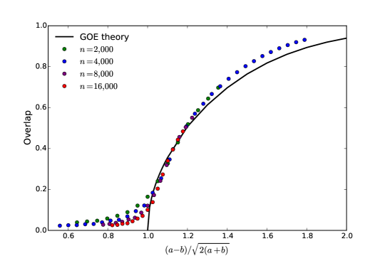
Figure 2: Community detection under the hidden partition model of Eq. (287), for average degree $(a+b)/2=5$. Dots corresponds to the performance of the SDP reconstruction method (averaged over $500$ realizations). The continuous curve is the asymptotic analytical prediction for the Gaussian model (which captures the large-degree behavior).

Figures 2 illustrates our results for the community detection problem under the hidden partition model of Eq. (287). Recall that we encode the ground truth by a vector $\bm{x_{0}}\in\{+1,-1\}^{n}$. In the present context, an estimator is required to return a partition of the vertices of the graph. Formally, it is a function on the space of graphs with $n$ vertices ${\mathcal{G}}_{n}$, namely $\bm{\hat{x}}:{\mathcal{G}}_{n}\to\{+1,-1\}^{n}$, $G\mapsto\bm{\hat{x}}(G)$. We will measure the performances of such an estimator through the overlap:

$${\rm Overlap}_{n}(\bm{\hat{x}})=\frac{1}{n}{\mathbb{E}}\big{\{}\big{|}\langle\bm{\hat{x}}(G),\bm{x_{0}}\rangle\big{|}\big{\}}\,.$$ (8)

and its asymptotic $n\to\infty$ limit (for which we omit the subscript). In order to motivate the SDP relaxation we note that the maximum likelihood estimator partitions $V$ in two sets of equal size as to minimize the number of edges across the partition (the minimum bisection problem). Formally

$$\bm{\hat{x}}^{\mbox{\tiny{ML}}}(G)\equiv\arg\!\!\max_{{\bm{x}}\in\{+1,-1\}^{n}}\Big{\{}\sum_{(i,j)\in E}x_{i}x_{j}:\;\;\;\langle{\bm{x}},{\mathbf{1}}\rangle=0\Big{\}}\,,$$ (9)

where ${\mathbf{1}}=(1,1,\dots,1)$ is the all-ones vector. Once more, this problem is hard to approximate [Kho06], which motivates the following SDP relaxation:

maximize $$\;\;\;\sum_{(i,j)\in E}X_{ij}\,,$$ (10)

subject to $$\;\;\;\bm{X}\succeq 0\,,\;\;\;\;\bm{X}{\mathbf{1}}={\mathbf{0}}\,,\;\;\;\;X_{ii}=1\;\;\forall i\in[n]\,.$$

Given an optimizer $\bm{X}_{\mbox{\tiny{opt}}}=\bm{X}_{\mbox{\tiny{opt}}}(G)$, we extract a partition of the vertices $V$ as follows. As for the ${\mathbb{Z}}_{2}$ synchronization problem, we compute the principal eigenvector ${\bm{v}}_{1}(\bm{X}_{\mbox{\tiny{opt}}})$. We then partition $V$ according to the sign of ${\bm{v}}_{1}(\bm{X}_{{\mbox{\tiny{opt}}}})$. Formally

$$\bm{\hat{x}}^{\mbox{\tiny{SDP}}}(G)={\rm sign}\big{(}{\bm{v}}_{1}(\bm{X}_{\mbox{\tiny{opt}}}(G))\big{)}\,.$$ (11)

Let us emphasize a few features of Figure 2:

1. Accuracy of GOE theory. The continuous curve of Figure 2 reports the analytical prediction within the ${\mathbb{Z}}_{2}$ synchronization model, with Gaussian noise (the GOE theory). This can be shown to capture the large degree limit: $d=(a+b)/2\to\infty$, with $\lambda=(a-b)/\sqrt{2(a+b)}$ fixed. However, it describes well the empirical results for sparse graphs of average degree as small as $d=5$.

2. Superiority of SDP to PCA. A sequence of recent papers (see [KMM⁺13] and references therein) demonstrate that classical spectral methods –such as PCA– fail to detect the hidden partition in graphs with bounded average degree. In contrast, Figure 2 shows that a standard SDP relaxation does not break down in the sparse regime. See [MS15] for rigorous evidence towards the same conclusion.

3. Near optimality of SDP. As proven in [MNS12], no estimator can achieve ${\rm Overlap}_{n}(\bm{\hat{x}})\geq\delta>0$ as $n\to\infty$, if $\lambda=(a-b)/\sqrt{2(a+b)}<1$.

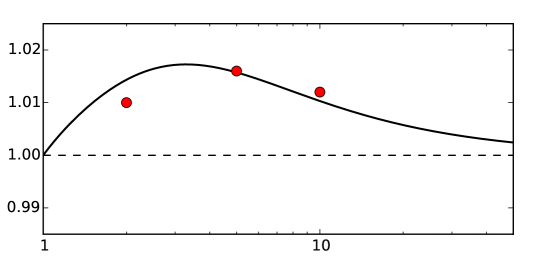
Figure 3: Continuous line: prediction for the critical point of the SDP estimator (in terms of the rescaled parameter $\lambda=(a-b)/\sqrt{2(a+b)}$). Dashed line: ideal phase transition $\lambda=1$. Red circles: numerical estimates of the phase transition location for $d=2$, $5$, $10$.

Figure 2 (and the theory developed in the next section) suggests that SDP has a phase transition threshold. Namely, there exists $\lambda_{c}^{\mbox{\tiny{SDP}}}=\lambda_{c}^{\mbox{\tiny{SDP}}}(d)$ such that, if

$$\lambda=\frac{a-b}{\sqrt{2(a+b)}}\geq\lambda_{c}^{\mbox{\tiny{SDP}}}\big{(}d=(a+b)/2\big{)}\,.$$ (12)

then SDP achieves overlap bounded away from zero: ${\rm Overlap}(\bm{\hat{x}}^{\mbox{\tiny{SDP}}})>0$. The figure also suggests $\lambda_{c}^{\mbox{\tiny{SDP}}}(5)\approx\lambda_{c}^{\mbox{\tiny{Bayes}}}=1$, i.e. SDP is nearly optimal.

Below we will derive an accurate approximation for the critical point $\lambda_{c}^{\mbox{\tiny{SDP}}}(d)$. The factor $\lambda_{c}^{\mbox{\tiny{SDP}}}(d)$ measures the sub-optimality of SDP for graphs of average degree $d$.

Figure 3 plots our prediction for the function $\lambda_{c}^{\mbox{\tiny{SDP}}}(d)$, together with empirically determined values for this threshold, obtained through Monte Carlo experiments for $d\in\{2,5,10\}$ (red circles). These were obtained by running the SDP estimator on randomly generated graphs with size up to $n=64,000$ (total CPU time was about $10$ years). In particular, we obtain $\lambda_{c}^{\mbox{\tiny{SDP}}}(d)>1$ strictly, but the gap $\lambda_{c}^{\mbox{\tiny{SDP}}}(d)-1$ is very small (at most of the order of $2\%$) for all $d$. This confirms in a precise quantitative way the conclusion that SDP is nearly optimal for the hidden partition problem.

Simulations results are in broad agreement with our predictions, but present small discrepancies (below $0.5\%$). These discrepancies might be due to the extrapolation form finite-$n$ simulations to $n\to\infty$, or to the inaccuracy of our analytical calculation.

3 Analytical results

Our analysis is based on a connection with statistical mechanics. The models arising from this connection are spin models in the so-called ‘large-$N$’ limit, a topic of intense study across statistical mechanics and quantum field theory [BW93]. Here we exploit this connection to apply non-rigorous but sophisticated tools from the theory of mean field spin glasses [MM09, MPV87]. The paper [MS15] provides partial rigorous evidence towards the predictions developed here.

We will first focus on the simpler problem of synchronization under Gaussian noise, treating together the ${\mathbb{Z}}_{2}$ and $U(1)$ case. We will then discuss the new features arising within the sparse hidden partition problem. Most technical derivations are presented in the SI. In order to treat the real (${\mathbb{Z}}_{2}$) and complex ($U(1)$) cases jointly, we will use ${\mathbb{F}}$ to denote any of the fields of reals or complex numbers, i.e. either ${\mathbb{R}}$ or ${\mathbb{C}}$.

3.1 Gibbs measures, vector spin models

We start by recalling that a matrix $\bm{X}\in{\mathbb{F}}^{n\times n}$ is PSD if and only if it can be written as $\bm{X}={\bm{\sigma}}{\bm{\sigma}}^{*}$ for some ${\bm{\sigma}}\in{\mathbb{F}}^{n\times m}$. Indeed, without loss of generality, one can take $m=n$, and any $m\geq n$ is equivalent.

Letting ${\bm{\sigma}}_{1}$, …${\bm{\sigma}}_{n}\in{\mathbb{F}}^{m}$ be the rows of ${\bm{\sigma}}$, the SDP (288) can be rewritten as

maximize $$\;\;\;\sum_{(i,j)}Y_{ij}\langle{\bm{\sigma}}_{i},{\bm{\sigma}}_{j}\rangle\,,$$ (13)

subject to $$\;\;\;{\bm{\sigma}}_{i}\in S^{m-1}\;\;\forall i\in[n]\,,$$

with $S^{m-1}=\{{\bm{z}}\in{\mathbb{F}}^{m}:\;\|{\bm{z}}\|_{2}=1\}$ the unit sphere in $m$ dimensions. The SDP relaxation corresponds to any case $m\geq n$ or –following the physics parlance– $m=\infty$. Note however that cases with bounded (small) $m$ are of independent interest. In particular, for $m=1$ we have ${\bm{\sigma}}_{i}\in\{-1,+1\}$ (for the real case) or ${\bm{\sigma}}_{i}\in U(1)\subset{\mathbb{C}}$ (for the complex case). Hence we recover the maximum-likelihood estimator setting $m=1$. It is also known that, for $m>\sqrt{2n}$, the problem (49) has no local optima except the global ones [BM03].

A crucial question is how the solution of (49) depends on the spin dimensionality $m$, for $m\ll n$. Denote by ${\rm OPT}(\bm{Y};m)$ the optimum value when the dimension is $m$ (in particular ${\rm OPT}(\bm{Y};m)$ is also the value of (288) for $m\geq n$). It was proven in [MS15] that there exists a constant $C$ independent of $m$ and $n$ such that

$$\Big{(}1-\frac{C}{m}\Big{)}\,{\rm OPT}(\bm{Y};\infty)\leq{\rm OPT}(\bm{Y};m)\leq{\rm OPT}(\bm{Y};\infty)\,,$$ (14)

with probability converging to one as $n\to\infty$ (whereby $\bm{Y}$ is chosen with any of the distributions studied in the present paper). The upper bound in Eq. (14) follows immediately from the definition. The lower bound is a generalization of the celebrated Grothendieck inequality from functional analysis [KN12].

The above inequalities imply that we can obtain information about the SDP (288) in the $n\to\infty$ limit, by taking $m\to\infty$ after $n\to\infty$. This is the asymptotic regime usually studied in physics under the term ‘large-$N$ limit.’

Finally, we can associate to the problem (49) a finite-temperature Gibbs measure as follows:

$$p_{\beta,m}({\rm d}{\bm{\sigma}})=\frac{1}{Z}\exp\Big{\{}2m\beta\sum_{i<j}\Re(Y_{ij}\langle{\bm{\sigma}}_{i},{\bm{\sigma}}_{j}\rangle)\Big{\}}\,\prod_{i=1}^{n}p_{0}({\rm d}{\bm{\sigma}}_{i})\,.$$ (15)

where $p_{0}({\rm d}{\bm{\sigma}}_{i})$ is the uniform measure over the $m$-dimensional sphere $S^{m-1}$, and $\Re(z)$ denotes the real part of $z$. This allows to treat in a unified framework all of the estimators introduced above. The optimization problem (49) is recovered by taking the limit $\beta\to\infty$ (with maximum likelihood for $m=1$ and SDP for $m\to\infty$). The Bayes-optimal estimator is recovered by setting $m=1$ and $\beta=\lambda/2$ (in the real case) or $\beta=\lambda$ (in the complex case).

3.2 Cavity method: ${\mathbb{Z}}_{2}$ and $U(1)$ synchronization

The cavity method from spin-glass theory can be used to analyze the asymptotic structure of the Gibbs measure (42) as $n\to\infty$. Below we will state the predictions of our approach for the SDP estimator $\bm{\hat{x}}^{\mbox{\tiny{SDP}}}$.

Here we list the main steps of our analysis for the expert reader, deferring a complete derivation to the SI:

• We use the cavity method to derive the ‘replica symmetric’ predictions for the model (42) in the limit $n\to\infty$.

• By setting $m=1$, $\beta=\lambda/2$ (in the real case) or $\beta=\lambda$ (in the complex case) we obtain the Bayes-optimal error ${\rm MSE}(\bm{\hat{x}}^{\mbox{\tiny{Bayes}}})$: on the basis of [DAM15], we expect the replica symmetric assumption to hold, and these predictions to be exact. (See also [LKZ15] for related work.)

• By setting $m=1$ and $\beta\to\infty$ we obtain a prediction for the error of maximum likelihood estimation ${\rm MSE}(\bm{\hat{x}}^{\mbox{\tiny{ML}}})$. While this prediction is not expected to be exact (because of replica symmetry breaking), it should be nevertheless rather accurate, especially for large $\lambda$.

• By setting $m\to\infty$ and $\beta\to\infty$, we obtain the SDP estimation error ${\rm MSE}(\bm{\hat{x}}^{\mbox{\tiny{SDP}}})$, which is our main object of interest. Notice that the inversion of limits $m\to\infty$ and $n\to\infty$ is justified (at the level of objective value) by Grothendieck inequality. Further, since the $m=\infty$ case is equivalent to a convex program, we expect the replica symmetric prediction to be exact in this case.

The properties of the SDP estimator are given in terms of the solution of a set 3 non-linear equations for the 3 scalar parameters $\mu$, $q$, $b\in{\mathbb{R}}$, that we state next. Let $Z\sim{\sf N}(0,1)$ (in the real case) or $Z\sim{\sf CN}(0,1)$ (in the complex case). Define $\rho=\rho(Z;\mu,q,r)$ as the only non-negative solution of the following equation in $(0,\infty)$:

$$1=\frac{|\mu+\sqrt{q}Z|^{2}}{(\rho+r)^{2}}+\frac{1-q}{\rho^{2}}\,.$$ (16)

Then $\mu$, $q$, $r$ satisfy

$$\mu =\lambda{\mathbb{E}}\left\{\frac{\mu+\sqrt{q}\,\Re(Z)}{\rho+r}\right\}\,,\;\;\;\;\;\;\;q={\mathbb{E}}\left\{\frac{|\mu+\sqrt{q}\,Z|^{2}}{(\rho+r)^{2}}\right\}\,,$$ (17)

$$r ={\mathbb{E}}\Big{\{}\frac{1}{\rho}-\frac{\mu}{\sqrt{q}}\,\frac{\Re(Z)}{\rho+r}-\frac{|Z|^{2}}{\rho+r}\Big{\}}\,.$$ (18)

These equations can be solved by iteration, after approximating the expectations on the right-hand side numerically. The properties of the SDP estimator can be derived from this solution. Concretely, we have

$${\rm MSE}(\bm{\hat{x}}^{\mbox{\tiny{SDP}}})=1-\frac{\mu(\lambda)^{2}}{\lambda^{2}q(\lambda)}\,.$$ (19)

The corresponding curve is reported in Figure 1 for the real case ${\mathfrak{G}}={\mathbb{Z}}_{2}$. We can also obtain the asymptotic overlap from the solution of these equations. The cavity prediction is

$${\rm Overlap}(\bm{\hat{x}}^{\mbox{\tiny{SDP}}})=1-2\Phi\Big{(}-\frac{\mu(\lambda)}{\sqrt{q(\lambda)}}\Big{)}\,.$$ (20)

The corresponding curve is plotted in Figure 2.

More generally, for any dimension $m$, and inverse temperature $\beta$, we obtain equations that are analogous to Eqs. (17)-(18). The parameters $\mu,q,b$ characterize the asymptotic structure of the probability measure $p_{\beta,m}({\rm d}{\bm{\sigma}})$ defined in Eq. (42), as follows. We assume, for simplicity $\bm{x_{0}}=(+1,\dots,+1)$. Define the following probability measure on unit sphere $S^{m-1}$, parametrized by ${\bm{\xi}}\in{\mathbb{R}}^{m}$, $r\in{\mathbb{R}}$

$$\nu_{{\bm{\xi}},r}({\rm d}{\bm{\sigma}})=\frac{1}{z({\bm{\xi}},r)}\,\exp\Big{\{}2\beta\,m\Re\langle{\bm{\xi}},{\bm{\sigma}}\rangle-\beta\,m\,r|\sigma_{1}|^{2}\Big{\}}\,p_{0}({\rm d}{\bm{\sigma}})\,,$$ (21)

For $\nu$ a probability measure on $S^{m-1}$ and $R$ an orthogonal (or unitary) matrix, let $\nu^{R}$ be the measure obtained by ‘rotating’ $\nu$. Finally, let $p^{(m,\beta)}_{i(1),\dots,i(k)}$ denote the joint distribution of ${\bm{\sigma}}_{i(1)},\cdots,{\bm{\sigma}}_{i(k)}$ under $p_{m,\beta}$. Then, for any fixed $k$, and any sequence of $k$-uples $(i(1),\dots,i(k))_{n}\in[n]$, we have

$$p^{(m,\beta)}_{i(1),\dots,i(k)}\Rightarrow\int\nu^{R}_{{\bm{\xi}}_{1},r}(\,\cdot\,)\times\cdots\times\nu^{R}_{{\bm{\xi}}_{k},r}(\,\cdot\,)\,{\rm d}R$$ (22)

Here ${\rm d}R$ denotes the uniform (Haar) measure on the orthogonal group, $\Rightarrow$ denotes convergence in distribution (note that $p^{(m,\beta)}_{i(1),\dots,i(k)}$ is a random variable), and ${\bm{\xi}}_{1},\dots,{\bm{\xi}}_{k}\sim_{iid}{\sf N}(\mu\,{\bm{e}}_{1},{\bm{Q}})$ with ${\bm{Q}}={\rm diag}(q,q_{0}\dots,q_{0})$, $q_{0}=(1-q)/(m-1)$.

3.3 Cavity method: Community detection in sparse graphs

We next consider the hidden partition model, defined by Eq. (287). As above, we denote by $d=(a+b)/2$ the asymptotic average degree of the graph $G$, and by $\lambda=(a-b)/\sqrt{2(a+b)}$ the ‘signal-to-noise’ ratio. As illustrated by Figure 2 (and further simulations presented in SI), ${\mathbb{Z}}_{2}$ synchronization appears to be a very accurate approximation for the hidden partition model already at moderate $d$.

The main change with respect to the dense case is that the phase transition at $\lambda=1$, is slightly shifted, as per Eq. (12). Namely, SDP can detect the hidden partition with high probability if and only if $\lambda\geq\lambda_{c}^{\mbox{\tiny{SDP}}}(d)$, for some $\lambda_{c}^{\mbox{\tiny{SDP}}}(d)>1$.

Our prediction for the curve $\lambda_{c}^{\mbox{\tiny{SDP}}}(d)$ will be denoted by $\tilde{\lambda}_{c}^{\mbox{\tiny{SDP}}}(d)$ and is plotted in Figure 3. It is obtained by finding an approximate solution of the RS cavity equations. We see that $\tilde{\lambda}_{c}^{\mbox{\tiny{SDP}}}(d)$ approaches very quickly the ideal value $\lambda=1$ for $d\to\infty$. Indeed our prediction implies

$$\tilde{\lambda}_{c}^{\mbox{\tiny{SDP}}}(d)=1+\frac{1}{8d}+O(d^{-2})\,.$$ (23)

Also, $\tilde{\lambda}_{c}^{\mbox{\tiny{SDP}}}(d)\to 1$ as $d\to 1$. This is to be expected because the constraints $a\geq b\geq 0$ imply $(a-b)/2\leq d$, with $b=0$ at $(a-b)/2=d$. Hence the community detection problem becomes trivial at $(a-b)/2=d$: it is sufficient to identify the connected components in $G$. This implies the bound $\lambda_{c}^{\mbox{\tiny{SDP}}}(d)\leq\sqrt{d}$.

More interestingly, $\tilde{\lambda}_{c}^{\mbox{\tiny{SDP}}}(d)$ admits a characterization in terms of a distributional recursion, that can be evaluated numerically, and is plotted as a continuous line in Figure 3. Surprisingly, the SDP detection threshold appears to be sub-optimal at most by $2\,\%$. In order to state this characterization, consider first the recursive distributional equation (RDE)

$${\sf c}\stackrel{{\scriptstyle{\rm d}}}{{=}}\sum_{i=1}^{L}\frac{{\sf c}_{i}}{1+{\sf c}_{i}}\,.$$ (24)

Here $\stackrel{{\scriptstyle{\rm d}}}{{=}}$ denotes equality in distribution, $L\sim{\rm Poisson}(d)$ and ${\sf c}_{1},\dots,{\sf c}_{L}$ are i.i.d. copies of ${\sf c}$. This has to be read as an equation for the law of the random variable ${\sf c}$ (see, e.g., [AB05] for further background on RDEs). We are interested in a specific solution of this equation, which can be constructed as follows. Set $c^{0}=\infty$ almost surely, and, for $\ell\geq 0$, let ${\sf c}^{\ell+1}\stackrel{{\scriptstyle{\rm d}}}{{=}}\sum_{i=1}^{L}{\sf c}_{i}^{\ell}/(1+{\sf c}^{\ell}_{i})$. It is proved in [LPP97] that the resulting sequence of random variables converges in distribution to a solution of Eq. (24): ${\sf c}^{\ell}\stackrel{{\scriptstyle{\rm d}}}{{\Rightarrow}}{\sf c}_{*}$.

The quantity ${\sf c}_{*}$ has a beautiful interpretation. Consider a (rooted) Galton-Watson tree with offspring distribution $d$, and imagine each edge to be a conductor with conductance equal to one. Then ${\sf c}_{*}$ is the total conductance between the root, and the boundary of the tree ‘at infinity.’ In particular, ${\sf c}_{*}=0$ almost surely for $d\leq 1$, and ${\sf c}_{*}>0$ with positive probability if $d>1$ (see [LP13] and SI).

Next consider the distributional recursion

$$\big{(}{\sf c}^{\ell+1};h^{\ell+1}\big{)}\stackrel{{\scriptstyle{\rm d}}}{{=}}\Big{(}\sum_{i=1}^{L_{+}+L_{-}}\frac{{\sf c}^{\ell}_{i}}{1+{\sf c}^{\ell}_{i}};\sum_{i=1}^{L_{+}+L_{-}}\frac{s_{i}h^{\ell}_{i}}{\sqrt{1+{\sf c}^{\ell}_{i}}}\Big{)}\,,$$ (25)

where $s_{1},\dots,s_{L_{+}}=+1$, $s_{L_{+}+1},\dots,s_{L_{+}+L_{-}}=-1$, and we use initialization $({\sf c}^{0},h^{0})=(+\infty,1)$. This recursion determines sequentially the distribution of $({\sf c}^{\ell+1},h^{\ell+1})$ from the distribution of $({\sf c}^{\ell},h^{\ell})$. Here $L_{+}\sim{\rm Poisson}((d+\lambda)/2)$, $L_{-}\sim{\rm Poisson}((d-\lambda)/2)$, and $({\sf c}^{\ell}_{1},h^{\ell}_{1}),\dots,({\sf c}^{\ell}_{L},h^{\ell}_{L})$ are i.i.d. copies of $({\sf c}^{\ell},h^{\ell})$, independent of $L_{+},L_{-}$. Notice that since $L_{+}+L_{-}\sim{\rm Poisson}(d)$, we have ${\sf c}^{\ell}\stackrel{{\scriptstyle{\rm d}}}{{\Rightarrow}}{\sf c}_{*}$. The threshold $\tilde{\lambda}_{c}^{\mbox{\tiny{SDP}}}(d)$ is defined as the smallest $\lambda$ such that the $h^{t}$ ‘diverges exponentially’:

$$\tilde{\lambda}_{c}^{\mbox{\tiny{SDP}}}(d)\equiv\inf\Big{\{}\lambda\in[0,\sqrt{d}]:\,\lim\inf_{t\to\infty}\frac{1}{t}\log{\mathbb{E}}(|h^{t}|^{2})>0\Big{\}}\,.$$ (26)

This value can be computed numerically, for instance by sampling the recursion (230). The results of such an evaluation are plotted as a continuous line in Figure 3.

4 Final algorithmic considerations

We have shown that ideas from statistical mechanics can be used to precisely locate phase transitions in SDP relaxations for high-dimensional statistical problems. In the problems investigated here, we find that SDP relaxations have optimal thresholds (in ${\mathbb{Z}}_{2}$ and $U(1)$ synchronization) or nearly-optimal thresholds (in community detection under the hidden partition model). Here ‘near-optimality’ is to be interpreted in a precise quantitative sense: SDP’s threshold is sub-optimal –at most– by a $2\,\%$ factor. As such SDPs provide a very useful tool for designing computationally efficient algorithms, that are also statistically efficient.

Let us emphasize that other polynomial-time algorithms can be used for the specific problems studied here. In the synchronization problem, naive PCA achieves the optimal threshold $\lambda=1$. In the community detection problem, several authors recently developed ingenious spectral algorithms that achieve the information theoretically optimal threshold $(a-b)/\sqrt{2(a+b)}=1$, see e.g. [DKMZ11, KMM⁺13, Mas14, MNS13, SKZ14].

However, SDP relaxations have the important feature of being robust to model miss-specifications (see also [MPW15] for an independent investigation of robustness issues). In order to illustrate this point, we perturbed the hidden partition model as follows. For a perturbation level $\alpha\in[0,1]$, we draw $n\alpha$ vertices $i_{1},\dots,i_{n\alpha}$ uniformly at random in $G$. For each such vertex $i_{\ell}$ we connect by edges all the neighbors of $i_{\ell}$. In our case, this results in adding $O(nd^{2}\alpha)$ edges.

In the SI, we compare the behavior of SDP and the Bethe Hessian algorithm of [SKZ14] for this perturbed model: while SDP appears to be rather insensitive to the perturbation, the performance of Bethe Hessian are severely degraded by it. We expect a similar fragility to arise in other spectral algorithms.

a

Supplementary Information

Most of the derivations in this documents are based on non-rigorous method from statistical physics. All the results that are rigorously proved will be stated as lemmas, propositions, and so on.

5 Notations

5.1 General notations

We will often treat ${\mathbb{Z}}_{2}$ and $U(1)$ synchronization simultaneously. Throughout ${\mathbb{F}}={\mathbb{R}}$ or ${\mathbb{F}}={\mathbb{C}}$ depending on whether we are treating the real case (${\mathbb{Z}}_{2}$ synchronization) or the complex case ($U(1)$ synchronization).

We let $S^{m-1}$ denotes the radius one sphere in ${\mathbb{R}}^{m}$ or ${\mathbb{C}}^{m}$ depending on the context. Namely $S^{m-1}=\{{\bm{z}}\in{\mathbb{F}}^{m}:\,\|{\bm{z}}\|_{2}=1\}$. In particular $S^{0}=\{+1,-1\}$ in the real case, and $S^{0}=\{z\in{\mathbb{C}}:|z|=1\}$ in the complex case.

Some of our formulae depends upon the domain that we are considering (real or complex). In order to write them in a compact form, we introduce the notation $s_{\mathfrak{G}}=1$ for ${\mathfrak{G}}={\mathbb{Z}}_{2}$, and $s_{\mathfrak{G}}=2$ for ${\mathfrak{G}}=U(1)$.

We write $X\sim{\rm Poisson}(a)$ to indicate that $X$ is a Poisson random variable with mean $a$. A Gaussian random vector ${\bm{z}}$ with mean ${\bm{a}}={\mathbb{E}}({\bm{z}})$ and covariance ${\bm{C}}={\mathbb{E}}(({\bm{z}}-{\bm{a}})({\bm{z}}-{\bm{a}})^{*})$ is denoted by ${\bm{z}}\sim{\sf N}({\bm{a}},{\bm{C}})$. Note that in the complex case, this means that ${\bm{C}}$ is Hermitian and ${\mathbb{E}}(({\bm{z}}-{\bm{a}})({\bm{z}}-{\bm{a}})^{{\sf T}})=0$. Occasionally, we will write ${\bm{z}}\sim{\sf CN}({\bm{a}},{\mathcal{C}})$ for complex Gaussians, whenever it is useful to emphasize that ${\bm{z}}$ is complex.

The standard Gaussian density is denoted by $\phi(x)=e^{-x^{2}/2}/\sqrt{2\pi}$, and the Gaussian distribution by $\Phi(x)=\int_{-\infty}^{x}\phi(t)\,{\rm d}t$.

Given two un-normalized measures $p$ and $q$ on the same space, we write $p(s)\cong q(s)$ if they are equal up to an overall normalization constant. We use $\doteq$ to denote equality up to subexponential factors, i.e. $f(n)\doteq g(n)$ if $\lim_{n\to\infty}n^{-1}\log[f(n)/g(n)]=0$.

5.2 Estimation metrics

We recall the definition of some estimation metrics used in the main text. For the sake of uniformity, we consider estimators $\bm{\hat{x}}:{\mathbb{R}}^{n\times n}\to{\mathbb{R}}^{n}$.

It is convenient to define a scaled MSE, with scaling factor $c\in{\mathbb{F}}$:

$${\rm MSE}_{n}(\bm{\hat{x}};c)\equiv\frac{1}{n}{\mathbb{E}}\big{\{}\min_{s\in S^{0}}\big{\|}\bm{x_{0}}-s\,c\,\bm{\hat{x}}(\bm{Y})\big{\|}^{2}_{2}\big{\}}\,.$$ (27)

We also define the overlap as follows in the real case

$${\rm Overlap}_{n}(\hat{x})\equiv\frac{1}{n}{\mathbb{E}}\big{\{}|\langle{\rm sign}(\bm{\hat{x}}(\bm{Y})),\bm{x_{0}}\rangle|\big{\}}\,.$$ (28)

In the complex case, we replace ${\rm sign}(z)$ by $z/|z|$ (defined to be $0$ at $z=0$):

$${\rm Overlap}_{n}(\hat{x})\equiv\frac{1}{n}{\mathbb{E}}\left\{\left|\sum_{i=1}^{n}\frac{\hat{x}_{i}(\bm{Y})}{|\hat{x}_{i}(\bm{Y})|}\,x_{0,i}\right|\right\}\,.$$ (29)

This formula applies to the real case as well. (Note that, in the main text, we defined the overlap only for estimators taking values in $\{+1,-1\}^{n}$, in the real case. Throughout these notes, we generalize that definition for the sake of uniformity.)

We omit the subscript $n$ to refer to the $n\to\infty$ limit of these quantities.

6 Preliminary facts

6.1 Some estimation identities

Lemma 6.1.

Let $p_{0}(\,\cdot\,)$ be a probability measure on the real line ${\mathbb{R}}$, symmetric around $0$ (i.e. $p_{0}((a,b))=p_{0}((-b,-a))$ for any interval $(a,b)$). For $\gamma\geq 0$, define $f:{\mathbb{R}}\to{\mathbb{R}}$ as

$$f(y;\gamma)\equiv\frac{\int\sigma\,e^{\sqrt{\gamma}y\sigma-\frac{1}{2}\gamma\sigma^{2}}\,p_{0}({\rm d}\sigma)}{\int e^{\sqrt{\gamma}y\sigma-\frac{1}{2}\gamma\sigma^{2}}\,p_{0}({\rm d}\sigma)}\,.$$ (30)

Then we have the identity

$${\mathbb{E}}\{|\sigma|\,f(\sqrt{\gamma}|\sigma|+Z;\gamma)\}={\mathbb{E}}\big{\{}f(\sqrt{\gamma}|\sigma|+Z;\gamma)^{2}\big{\}}\,.$$ (31)

where the expectation is with respect to the independent random variables $Z\sim{\sf N}(0,1)$, and $\sigma\sim p_{0}(\,\cdot\,)$.

Analogously, let $p_{0}(\,\cdot\,)$ be a probability measure on ${\mathbb{C}}$, symmetric under rotations (i.e. $p_{0}(e^{i\theta}R)=p_{0}(R)$, $p_{0}(R)=p_{0}(R^{*})$ for any Borel set $R\subseteq{\mathbb{C}}$ and any $\theta\in(0,2\pi]$). For $\gamma\geq 0$, define $f:{\mathbb{C}}\to{\mathbb{R}}$ as

$$f(y;\gamma)\equiv\frac{\int\sigma\,e^{2\sqrt{\gamma}\Re(y^{*}\sigma)-\gamma|\sigma|^{2}}\,p_{0}({\rm d}\sigma)}{\int e^{2\sqrt{\gamma}\Re(y^{*}\sigma)-\gamma|\sigma|^{2}}\,p_{0}({\rm d}\sigma)}\,.$$ (32)

Then we have the identity (with $Z\sim{\sf CN}(0,1)$ a complex normal)

$${\mathbb{E}}\{|\sigma|\,f(\sqrt{\gamma}|\sigma|+Z;\gamma)\}={\mathbb{E}}\big{\{}|f(\sqrt{\gamma}|\sigma|+Z;\gamma)|^{2}\big{\}}\,.$$ (33)

Proof.

Consider, to be definite, the real case, and define the observation model

$$Y=\sqrt{\gamma}\,\sigma+Z\,,$$ (34)

where $\sigma\sim p_{0}(\,\cdot\,)$ independent of the noise $Z\sim{\sf N}(0,1)$. Then a straightforward calculation shows that

$$f(y;\gamma)={\mathbb{E}}\{\sigma|Y=y\}\,.$$ (35)

Then, by the tower property of conditional expectation ${\mathbb{E}}\{\sigma\,f(Y;\gamma)\}={\mathbb{E}}\{f(Y;\gamma)^{2}\}$ or, equivalently

$${\mathbb{E}}\{\sigma\,f(\sqrt{\gamma}\,\sigma+Z;\gamma)\}={\mathbb{E}}\{f(\sqrt{\gamma}\,\sigma+Z;\gamma)^{2}\}\,.$$ (36)

The identity (31) follows by exploiting the symmetry of $p_{0}$, which implies $f(-y;\gamma)=-f(y;\gamma)$.

The proof follows a similar argument in the complex case. ∎

We apply the above lemma to specific cases that will be of interest to us. Below, ${\rm I}_{k}(z)$ denotes the modified Bessel function of the second kind. Explicitly, for $k$ integer, we have the integral representation

$${\rm I}_{k}(z)=\frac{1}{2\pi}\int_{0}^{2\pi}e^{z\cos\theta}\cos(k\theta)\,{\rm d}\theta\,.$$ (37)

Corollary 6.2.

For any $\gamma\geq 0$, we have the identities

$${\mathbb{E}}\big{\{}\tanh(\gamma+\sqrt{\gamma}\,Z)\big{\}} ={\mathbb{E}}\big{\{}\tanh(\gamma+\sqrt{\gamma}\,Z)^{2}\big{\}}\,,$$ (38)

$${\mathbb{E}}\left\{\frac{\gamma+\sqrt{\gamma}\,Z}{|\gamma+\sqrt{\gamma}\,Z|}\,\frac{{\rm I}_{1}(2|\gamma+\sqrt{\gamma}\,Z|)}{{\rm I}_{0}(2|\gamma+\sqrt{\gamma}\,Z|)}\right\} ={\mathbb{E}}\left\{\frac{{\rm I}_{1}(2|\gamma+\sqrt{\gamma}\,Z|)^{2}}{{\rm I}_{0}(2|\gamma+\sqrt{\gamma}\,Z|)^{2}}\right\}\,,$$ (39)

where the expectation is with respect to $Z\sim{\sf N}(0,1)$ (first line) or $Z\sim{\sf CN}(0,1)$ (second line).

Proof.

These follows from Lemma 6.1. For the first line we apply the real case (31) with $p_{0}=(1/2)\delta_{+1}+(1/2)\delta_{-1}$, whence

$$f(y;\gamma)=\tanh(\sqrt{\gamma}\,y)\,.$$ (40)

For the second line we apply the complex case (32) with $p_{0}$ the uniform measure over the unit circle. Consider the change of variables $y=|y|e^{j\phi}$ and $\sigma=e^{j(\phi+\theta)}$. Computing the curve integral, we have

$$f(y;\gamma) =\frac{\int_{0}^{2\pi}\,e^{j(\phi+\theta)}e^{2\sqrt{\gamma}|y|\cos(\theta)}{\rm d}\theta}{\int_{0}^{2\pi}\,e^{2\sqrt{\gamma}y\cos(\theta)}{\rm d}\theta}$$

$$=\frac{e^{j\phi}\int_{0}^{2\pi}\,e^{2\sqrt{\gamma}|y|\cos(\theta)}\cos(\theta){\rm d}\theta}{\int_{0}^{2\pi}\,e^{2\sqrt{\gamma}|y|\cos(\theta)}{\rm d}\theta}=\frac{y}{|y|}\frac{{\rm I}_{1}(2\sqrt{\gamma}|y|)}{{\rm I}_{0}(2\sqrt{\gamma}|y|)}\,,$$ (41)

where in the second equality we used the fact that $\int_{0}^{2\pi}e^{2\sqrt{\gamma}|y|\cos(\theta)}\sin(\theta){\rm d}\theta=0$. ∎

7 Analytical results for ${\mathbb{Z}}_{2}$ and and $U(1)$ synchronization

As explained in the main text, we are interested in the following probability measure over ${\bm{\sigma}}=({\bm{\sigma}}_{1},{\bm{\sigma}}_{2},\dots,{\bm{\sigma}}_{n})$, where ${\bm{\sigma}}_{i}\in S^{m-1}$:

$$p_{\beta,m}({\rm d}{\bm{\sigma}})=\frac{1}{Z_{n,\bm{Y}}(\beta,m)}\exp\Big{\{}2m\beta\sum_{i<j}\Re(Y_{ij}\langle{\bm{\sigma}}_{i},{\bm{\sigma}}_{j}\rangle)\Big{\}}\,\prod_{i=1}^{n}p_{0}({\rm d}{\bm{\sigma}}_{i})\,.$$ (42)

Here $p_{0}({\rm d}{\bm{\sigma}}_{i})$ is the uniform measure over ${\bm{\sigma}}_{i}\in S^{m-1}$.

We define a general $m,\beta$ estimator as follows.

1. In order to break the ${\mathcal{O}}(m)$ symmetry, we add a term $\beta\sum_{i=1}^{n}\langle\bm{h},{\bm{\sigma}}\rangle$ in the exponent of Eq. (42), for $\bm{h}$ an arbitrary small vector. It is understood throughout that $\|\bm{h}\|_{2}\to 0$ after $n\to\infty$.

   As is customary in statistical physics, we will not explicitly carry out calculations with the perturbation $\bm{h}\neq 0$, but only using this device to select the relevant solution at $\bm{h}=0$.

2. We compute the expectation

   $${\bm{z}}(\bm{Y};\beta,m)=\int{\bm{\sigma}}\;p_{\beta,m}({\rm d}{\bm{\sigma}})\,.$$ (43)

   Note that for $\beta\to\infty$ this amounts to maximizing the exponent term in equation (42).

3. Compute the empirical covariance

   $${\bm{\widehat{Q}}}\equiv\frac{1}{n}\sum_{i=1}^{n}{\bm{z}}_{i}{\bm{z}}_{i}^{*}\,.$$ (44)

   Let ${\bm{\widehat{u}}}$ be its principal eigenvector.

4. Return $\bm{\hat{x}}^{(\beta,m)}$

   $$\hat{x}_{i}^{(\beta,m)}=c\,\langle{\bm{\widehat{u}}},{\bm{z}}_{i}\rangle\,,$$ (45)

   where $c=c(\lambda)$ is the optimal scaling predicted by the asymptotic theory.

7.1 Derivation of the Gibbs measure

The Gibbs measure (42) encodes several estimators of interests. Here we briefly describe this connections.

Bayes-optimal estimators. As mentioned in the main text, this is obtained by setting $m=1$ and $\beta=\lambda/2$ (in the real case) or $\beta=\lambda$ (in the complex case). To see this, recall our observation model (for $i<j$)

$$Y_{ij}=\frac{\lambda}{n}x_{0,i}x_{0,j}^{*}+W_{ij}\,,$$ (46)

with $x_{0,i}\in S^{0}$ and $W_{ij}\sim{\sf N}(0,1/n)$. Hence, by an application of Bayes formula, the conditional density of $\bm{x_{0}}={\bm{\sigma}}\in{\mathbb{F}}^{n}$ given $\bm{Y}$ is becomes

$$p({\rm d}{\bm{\sigma}}|\bm{Y}) =\frac{1}{Z^{\prime}_{\bm{Y}}}\,\exp\Big{\{}-\frac{ns_{{\mathfrak{G}}}}{2}\sum_{i<j}\Big{|}Y_{ij}-\frac{\lambda}{n}\sigma_{i}\sigma_{j}^{*}\Big{|}^{2}\Big{\}}\,\prod_{i=1}^{n}p_{0}({\rm d}\sigma_{i})\,,$$ (47)

where we recall that $s_{{\mathfrak{G}}}=1$ for ${\mathfrak{G}}={\mathbb{Z}}_{2}$ (real case), and $s_{{\mathfrak{G}}}=2$ for ${\mathfrak{G}}=U(1)$ (complex case). Further, $p_{0}({\rm d}\sigma)$ denotes the uniform measure over $S^{0}\in{\mathbb{F}}$ (in particular, this is the uniform measure over $\{+1,-1\}$ for ${\mathfrak{G}}={\mathbb{Z}}_{2}$). Expanding the square and re-absorbing terms independent of ${\bm{\sigma}}$ in the normalization constant, we get

$$p({\rm d}{\bm{\sigma}}|\bm{Y}) =\frac{1}{Z_{\bm{Y}}}\,\exp\Big{\{}\lambda s_{{\mathfrak{G}}}\sum_{i<j}\Re(Y_{ij}\sigma_{i}^{*}\sigma_{j})\Big{\}}\,\prod_{i=1}^{n}p_{0}({\rm d}\sigma_{i})\,.$$ (48)

As claimed, this coincides with Eq. (42) if we set $\beta=\lambda/2$ (in the real case) or $\beta=\lambda$ (in the complex case).

Maximum-likelihood and SDP estimators. By letting $\beta\to\infty$ in Eq. (42), we obtain that $p_{\beta,m}$ concentrates on the maximizers of the problem

maximize $$\;\;\;\sum_{i<j}Y_{ij}\langle{\bm{\sigma}}_{i},{\bm{\sigma}}_{j}\rangle\,,$$ (49)

subject to $$\;\;\;{\bm{\sigma}}_{i}\in S^{m-1}\;\;\forall i\in[n]\,,$$

In the case $m\geq n$ we recover the SDP relaxation. In the case $m=1$, this is equivalent to the maximum likelihood problem

maximize $$\;\;\;\sum_{i<j}\big{|}Y_{ij}-\sigma_{i}\sigma_{j}^{*}\big{|}^{2}\,,$$ (50)

subject to $$\;\;\;\sigma_{i}\in S^{0}\;\;\forall i\in[n]\,.$$

7.2 Cavity derivation for ${\mathbb{Z}}_{2}$ and $U(1)$ synchronization

In this section we use the cavity method to derive the asymptotic properties of the measure (42).

7.2.1 General $m$ and $\beta$

In the replica-symmetric cavity method, we consider adding a single variable ${\bm{\sigma}}_{0}$ to a problem with $n$ variables ${\bm{\sigma}}_{1},{\bm{\sigma}}_{2},\dots,{\bm{\sigma}}_{n}$. We compute the marginal distribution of ${\bm{\sigma}}_{0}$ in the system with $n+1$ variables, to be denoted by $\nu^{n+1}_{0}({\rm d}{\bm{\sigma}}_{0})$. This is expressed in terms of the marginals of the other variables in the system with $n$ variables $\nu^{n}_{1}({\rm d}{\bm{\sigma}}_{0})$, …$\nu^{n}_{n}({\rm d}{\bm{\sigma}}_{1})$. We will finally impose the consistency condition that $\nu^{n+1}_{0}$ is distributed as any of $\nu^{n}_{1}$, …$\nu^{n}_{n}$ in the $n\to\infty$ limit.

Assuming that ${\bm{\sigma}}_{1}$, …${\bm{\sigma}}_{n}$ are, for this purpose, approximately independent, we get

$$\nu^{n+1}_{0}({\rm d}{\bm{\sigma}}_{0})\;\cong\;p_{0}({\rm d}{\bm{\sigma}}_{0})\prod_{k=1}^{n}\int\exp\Big{\{}2\beta m\Re(Y_{0k}\langle{\bm{\sigma}}_{0},{\bm{\sigma}}_{k}\rangle)\Big{\}}\;\nu^{n}_{k}({\rm d}{\bm{\sigma}}_{k})\,.$$ (51)

We will hereafter drop the superscripts $n$, $n+1$ assuming they will be clear from the range of the subscripts.

Next we consider a fixed $k\in[n]$ and estimate the integral by expanding the exponential term. This expansion proceeds slightly different in the real and the complex cases. We give details for the first one, leaving the second to the reader. Write

$$\int\exp\Big{\{}2\beta mY_{0k}\langle{\bm{\sigma}}_{0},{\bm{\sigma}}_{k}\rangle)\Big{\}}\;\nu_{k}({\rm d}{\bm{\sigma}}_{k})=$$

$$=1+2\beta mY_{0k}\langle{\bm{\sigma}}_{0},{\rm E}_{k}({\bm{\sigma}}_{k})\rangle+\frac{1}{2}\,4\beta^{2}m^{2}Y^{2}_{0k}\langle{\bm{\sigma}}_{0},{\rm E}_{k}({\bm{\sigma}}_{k}{\bm{\sigma}}_{k}^{*}){\bm{\sigma}}_{0}\rangle+O(n^{-3/2})$$

$$=\exp\Big{\{}2\beta mY_{0k}\langle{\bm{\sigma}}_{0},{\rm E}_{k}({\bm{\sigma}}_{k})\rangle+\frac{1}{2}\,4\beta^{2}m^{2}Y^{2}_{0k}\langle{\bm{\sigma}}_{0},\big{(}{\rm E}_{k}({\bm{\sigma}}_{k}{\bm{\sigma}}_{k}^{*})-{\rm E}_{k}({\bm{\sigma}}_{k}){\rm E}_{k}({\bm{\sigma}}_{k}^{*})\big{)}{\bm{\sigma}}_{0}\rangle+O(n^{-3/2})\Big{\}}\,,$$

where ${\rm E}_{k}(\,\cdot\,)\equiv\int(\,\cdot\,)\,\nu_{k}({\rm d}{\bm{\sigma}}_{k})$ denotes expectation with respect to $\nu_{k}$. Here, we used the fact that $Y_{ij}=O(1/\sqrt{n})$, as per equation (46).

Substituting in Eq. (51), and neglecting $O(n^{-1/2})$ terms, we get (both in the real and complex case)

$$\nu_{i}({\rm d}{\bm{\sigma}}_{i})=\frac{1}{z_{i}}\,\exp\Big{\{}2\beta\,m\,\Re\langle{\bm{\xi}}_{i},{\bm{\sigma}}_{i}\rangle+\frac{2\beta m}{s_{{\mathfrak{G}}}}\,\langle{\bm{\sigma}}_{i},{\bm{C}}_{i}{\bm{\sigma}}_{i}\rangle\Big{\}}\,p_{0}({\rm d}{\bm{\sigma}}_{i})\,\,,$$ (52)

where ${\bm{\xi}}_{i}\in{\mathbb{F}}^{m}$, ${\bm{C}}_{i}\in{\mathbb{F}}^{m\times m}$, with ${\bm{C}}_{i}^{*}={\bm{C}}_{i}$, $z_{i}$ is a normalization constant, and $s_{{\mathfrak{G}}}=1$ (real case) or $s_{{\mathfrak{G}}}=2$ (complex case). This expression holds for $i=0$ and, by the consistency condition, for all $i\in\{1,\dots,n\}$.

We further have the following equations for ${\bm{\xi}}_{0}$, ${\bm{C}}_{0}$:

$${\bm{\xi}}_{0} =\sum_{k=1}^{n}Y^{*}_{0k}{\rm E}_{k}({\bm{\sigma}}_{k})\,,$$ (53)

$${\bm{C}}_{0} =\beta m\sum_{k=1}^{n}|Y_{0k}|^{2}\big{(}{\rm E}_{k}({\bm{\sigma}}_{k}{\bm{\sigma}}_{k}^{*})-{\rm E}_{k}({\bm{\sigma}}_{k}){\rm E}_{k}({\bm{\sigma}}_{k}^{*})\big{)}\,.$$ (54)

Notice that the expectations ${\rm E}_{k}(\,\cdot\,)$ on the right-hand side are in fact functions of ${\bm{\xi}}_{k}$, ${\bm{C}}_{k}$ through Eq. (52).

We next pass to studying the distribution of $\{{\bm{\xi}}_{k}\}$ and $\{{\bm{C}}_{k}\}$. For large $n$, the pairs $\{({\bm{\xi}}_{k},{\bm{C}}_{k})\}$ appearing on the right-hand side of Eqs. (53), (54) can be treated as independent. By the law of large numbers and central limit theorem, we obtain that

$${\bm{\xi}}_{i}\sim{\sf N}({\bm{\mu}},{\bm{Q}})\,,\;\;\;\;\;{\bm{C}}_{i}={\bm{C}}\,,$$ (55)

for some deterministic quantities ${\bm{\mu}}$, ${\bm{Q}}$, ${\bm{C}}$. Note that the law of ${\bm{\xi}}_{i}$ can be equivalently described by

$${\bm{\xi}}_{i}={\bm{\mu}}+{\bm{Q}}^{1/2}{\bm{g}}\,,$$ (56)

where ${\bm{g}}=(g_{1},g_{2},\dots,g_{m})\sim{\sf N}(0,{\rm I}_{m})$.

Using these and the consistency condition in Eqs. (53), (54), we obtain the following equations for the unknowns ${\bm{\mu}},{\bm{Q}},{\bm{C}}$:

$${\bm{\mu}} =\lambda{\mathbb{E}}\big{\{}{\rm E}_{{\bm{\xi}},{\bm{C}}}({\bm{\sigma}})\big{\}}\,,$$ (57)

$${\bm{Q}} ={\mathbb{E}}\big{\{}{\rm E}_{{\bm{\xi}},{\bm{C}}}({\bm{\sigma}}){\rm E}_{{\bm{\xi}},{\bm{C}}}({\bm{\sigma}})^{*}\big{\}}\,,$$ (58)

$${\bm{C}} =\beta m\,{\mathbb{E}}\big{\{}{\rm E}_{{\bm{\xi}},{\bm{C}}}({\bm{\sigma}}{\bm{\sigma}}^{*})-{\rm E}_{{\bm{\xi}},{\bm{C}}}({\bm{\sigma}}){\rm E}_{{\bm{\xi}},{\bm{C}}}({\bm{\sigma}})^{*}\big{\}}\,.$$ (59)

Here ${\mathbb{E}}$ denotes expectation with respect to ${\bm{\xi}}\sim{\sf N}({\bm{\mu}},{\bm{Q}})$. Further ${\rm E}_{{\bm{\xi}},{\bm{C}}}$ denotes expectation with respect to the following probability measure on $S^{m-1}$:

$$\nu_{{\bm{\xi}},{\bm{C}}}({\rm d}{\bm{\sigma}})=\frac{1}{z({\bm{\xi}},{\bm{C}})}\,\exp\Big{\{}2\beta\,m\Re\langle{\bm{\xi}},{\bm{\sigma}}\rangle+\frac{2\beta\,m}{s_{{\mathfrak{G}}}}\langle{\bm{\sigma}},{\bm{C}}{\bm{\sigma}}\rangle\Big{\}}\,p_{0}({\rm d}{\bm{\sigma}})\,.$$ (60)

The prediction of the replica-symmetric cavity methods have been summarized in the main text. We generalize the discussion here. Assume, for simplicity $\bm{x_{0}}=(+1,\dots,+1)$. For $\nu$ a probability measure on $S^{m-1}$ and $R$ an orthogonal (or unitary) matrix, let $\nu^{R}$ be the measure obtained by ‘rotating’ $\nu$, i.e. $\nu^{R}({\bm{\sigma}}\in A)\equiv\nu(R^{-1}{\bm{\sigma}}\in A)$ for any measurable set $A$. Finally, let $p^{(m,\beta)}_{i(1),\dots,i(k)}$ denote the joint distribution of ${\bm{\sigma}}_{i(1)},\cdots,{\bm{\sigma}}_{i(k)}$ under $p_{m,\beta}$. Then, for any fixed $k$, and any sequence of $k$-tuples $(i(1),\dots,i(k))_{n}\in[n]$, we have

$$p^{(m,\beta)}_{i(1),\dots,i(k)}\Rightarrow\int\nu^{R}_{{\bm{\xi}}_{1},{\bm{C}}}(\,\cdot\,)\times\cdots\times\nu^{R}_{{\bm{\xi}}_{k},{\bm{C}}}(\,\cdot\,)\,{\rm d}R$$ (61)

Here ${\rm d}R$ denotes the uniform (Haar) measure on the orthogonal group, ‘$\Rightarrow$’ denotes convergence in distribution, and ${\bm{\xi}}_{1},\dots,{\bm{\xi}}_{k}\sim_{iid}{\sf N}(\mu,{\bm{Q}})$ as above. Note that the original measure (42) is unaltered under multiplication by a phase. Specifically, if we add an arbitrary phase $\phi_{\ell}$ to coordinate $\ell$ of the spins, the measure remains unchanged. In order to break this invariance, we consider marginals $\nu_{{\bm{\xi}},{\bm{C}}}$ that corresponds to ${\bm{\mu}}$ being real-valued. Henceforth, without loss of generality we stipulate that ${\bm{\mu}}$ is a real-valued vector.

While in general this prediction is only a good approximation (because of replica symmetry breaking) we expect to be asymptotically exact for the Bayes-optimal, ML and SDP estimator. In the next sections we will discuss special estimators.

7.2.2 Bayes-optimal: $m=1$ and $\beta\in\{\lambda/2,\lambda\}$

For $m=1$, ${\bm{\sigma}}=\sigma$ is a scalar satisfying $\sigma\sigma^{*}=|\sigma|^{2}=1$. Hence, the term proportional to ${\bm{C}}$ in Eq. (60) is a constant and can be dropped. Also ${\bm{\xi}}=\xi$, ${\bm{\mu}}=\mu$ and ${\bm{Q}}=q$ are scalar in this case.

The expression (60) thus reduces to

$$\nu_{\xi}({\rm d}\sigma)=\frac{1}{z(\xi)}\,e^{2\beta\,\Re(\xi^{*}\sigma)}\,p_{0}({\rm d}\sigma)\,,$$ (62)

with $p_{0}({\rm d}\sigma)$ the uniform measure on $\{+1,-1\}$ (in the real case) or on $\{z\in{\mathbb{C}}:\;|z|=1\}$ (in the complex case). Substituting in Eqs. (57), (58), we get

$$\mu =\lambda{\mathbb{E}}\big{\{}{\rm E}_{\xi}(\sigma)\big{\}}\,,$$ (63)

$$q ={\mathbb{E}}\big{\{}|{\rm E}_{\xi}(\sigma)|^{2}\big{\}}\,,$$ (64)

with ${\rm E}_{\xi}$ denoting expectation with respect to $\nu_{\xi}$, and ${\mathbb{E}}$ expectation with respect to $\xi\sim{\sf N}(\mu,q)$.

We will write these equations below in terms of classical functions both in the real and in the complex cases. Before doing that, we derive expressions for the estimation error in the $n\to\infty$ limit. The estimator $\bm{\hat{x}}(\bm{Y})$ is given in this case by $\bm{\hat{x}}(\bm{Y})=\bm{\hat{x}}^{\beta,m=1}(\bm{Y})$, cf. Eq. (43). Therefore, the scaled MSE, cf. Eq. (27), reads

$${\rm MSE}(\bm{\hat{x}};c) =\lim_{n\to\infty}\left\{1-\frac{2c}{n}\sum_{i=1}^{n}{\mathbb{E}}\big{\{}\Re(x_{0,i}\hat{x}_{i}(\bm{Y}))\big{\}}+\frac{c^{2}}{n}\sum_{i=1}^{n}{\mathbb{E}}\big{\{}|\hat{x}_{i}(\bm{Y})|^{2}\big{\}}\right\}$$ (65)

$$=1-2c{\mathbb{E}}\big{\{}\Re{\rm E}_{\xi}(\sigma)\big{\}}+c^{2}{\mathbb{E}}\big{\{}|{\rm E}_{\xi}(\sigma)|^{2}\big{\}}$$ (66)

$$=1-\frac{2c\mu}{\lambda}+c^{2}q\,.$$ (67)

Note that the optimal scaling is $c=\mu/(\lambda q)$, leading to minimal error –for the ideally scaled estimator–

$${\rm MSE}(\bm{\hat{x}}) =1-\frac{\mu^{2}}{\lambda^{2}q}\,.$$ (68)

For the overlap we have, from Eq. (29),

$${\rm Overlap}(\hat{x}) =\lim_{n\to\infty}\frac{1}{n}{\mathbb{E}}\left\{\left|\sum_{i=1}^{n}\frac{\hat{x}_{i}(\bm{Y})}{|\hat{x}_{i}(\bm{Y})|}\,x_{0,i}\right|\right\}$$ (69)

$$={\mathbb{E}}\Big{\{}\frac{{\rm E}_{\xi}(\sigma)}{|{\rm E}_{\xi}(\sigma)|}\Big{\}}\,.$$ (70)

Real case. In this case ${\rm E}_{\xi}(\sigma)=\tanh(2\beta\xi)$ and therefore Eqs. (63), (64) yield

$$\mu =\lambda{\mathbb{E}}\big{\{}\tanh\big{(}2\beta\mu+2\beta\sqrt{q}Z\big{)}\big{\}}\,,$$ (71)

$$q ={\mathbb{E}}\big{\{}\tanh\big{(}2\beta\mu+2\beta\sqrt{q}Z\big{)}^{2}\big{\}}\,,$$ (72)

where expectation is with respect to $Z\sim{\sf N}(0,1)$. As discussed in Section 7.1, the Bayes optimal estimator is recovered by setting $\beta=\lambda/2$ above. Using the identity (38) in Corollary 6.2, we obtain the solution

$$\mu=\frac{\kappa}{\lambda}\,,\;\;\;\;\;q=\frac{\kappa}{\lambda^{2}}\,.$$ (73)

where $\kappa$ satisfies the fixed point equation

$$\kappa=\lambda^{2}{\mathbb{E}}\big{\{}\tanh\big{(}\kappa+\sqrt{\kappa}Z\big{)}\big{\}}$$ (74)

We denote by $\kappa_{*}=\kappa_{*}(\lambda)$ the largest non-negative solution of this equation. Using Eqs. (67) and (70) we obtain the following predictions for the asymptotic estimation error

$${\rm MSE}(\bm{\hat{x}}^{\mbox{\tiny{Bayes}}}) =1-\frac{\kappa_{*}(\lambda)}{\lambda^{2}}\,,$$ (75)

$${\rm Overlap}(\bm{\hat{x}}^{\mbox{\tiny{Bayes}}}) =1-2\Phi(-\sqrt{\kappa_{*}(\lambda)})\,.$$ (76)

(Note that in this case, the optimal choice of a scaling is $c=1$.)

Complex case. In this case

$${\rm E}_{\xi}(\sigma)=\frac{\xi}{|\xi|}\,\frac{{\rm I}_{1}(2\beta|\xi|)}{{\rm I}_{0}(2\beta|\xi|)}\,,$$ (77)

where, as mentioned above, ${\rm I}_{k}(z)$ denotes the modified Bessel function of the second kind.

The general fixed point equations (63) and (64) yield

$$\mu =\lambda{\mathbb{E}}\Big{\{}\frac{\mu+\sqrt{q}\Re(Z)}{|\mu+\sqrt{q}Z|}\,\frac{{\rm I}_{1}(2\beta|\mu+\sqrt{q}Z|)}{{\rm I}_{0}(2\beta|\mu+\sqrt{q}Z|)}\Big{\}}\,,$$ (78)

$$q =\lambda{\mathbb{E}}\Big{\{}\frac{{\rm I}_{1}(2\beta|\mu+\sqrt{q}Z|)^{2}}{{\rm I}_{0}(2\beta|\mu+\sqrt{q}Z|)^{2}}\Big{\}}\,.$$ (79)

As discussed in Section 7.1, the Bayes optimal estimator is recovered by setting $\beta=\lambda$ in these equations. In this case we can use the identity (39) in Corollary 6.2, to obtain the solution

$$\mu=\frac{\kappa}{\lambda}\,,\;\;\;\;\;q=\frac{\kappa}{\lambda^{2}}\,.$$ (80)

where $\kappa$ satisfies the fixed point equation

$$\kappa=\lambda^{2}{\mathbb{E}}\Big{\{}\frac{\kappa+\sqrt{\kappa}\Re(Z)}{|\kappa+\sqrt{\kappa}Z|}\,\frac{{\rm I}_{1}(2|\kappa+\sqrt{\kappa}Z|)}{{\rm I}_{0}(2|\kappa+\sqrt{\kappa}Z|)}\Big{\}}\,,$$ (81)

where the expectation is taken with respect to $Z\sim{\sf CN}(0,1)$. We denote by $\kappa_{*}=\kappa_{*}(\lambda)$ the largest non-negative solution of these equations.

Using again Eqs. (67) and (70) , we obtain

$${\rm MSE}(\bm{\hat{x}}^{\mbox{\tiny{Bayes}}}) =1-\frac{\kappa_{*}(\lambda)}{\lambda^{2}}\,,$$ (82)

$${\rm Overlap}(\bm{\hat{x}}^{\mbox{\tiny{Bayes}}}) ={\mathbb{E}}\Big{\{}\frac{\kappa_{*}(\lambda)+\sqrt{\kappa_{*}(\lambda)}\,\Re(Z)}{|\kappa_{*}(\lambda)+\sqrt{\kappa_{*}(\lambda)}Z|}\Big{\}}\,.$$ (83)

7.2.3 Maximum likelihood: $m=1$ and $\beta\to\infty$

As discussed in Section 7.1, the maximum likelihood estimator is recovered by setting $m=1$ and $\beta\to\infty$. Notice that in this case our results are only approximate because of replica symmetry breaking.

We can take the limit $\beta\to\infty$ in Eqs. (62), (63), (64). In this limit, the measure $\nu_{\xi}(\,\cdot\,)$ concentrates on the single point $\sigma^{*}=\xi/|\xi|\in S^{0}$. We thus obtain

$$\mu =\lambda{\mathbb{E}}\Big{\{}\frac{\Re(\xi)}{|\xi|}\Big{\}}\,,$$ (84)

$$q =1\,.$$ (85)

We next specialize our discussion to the real and complex cases.

Real case. Specializing Eq. (84) to the real case, we get the equation

$$\mu =\lambda\big{(}1-2\Phi(-\mu)\big{)}\,.$$ (86)

Taylor expanding near $\mu=0$, this yields $\mu=2\phi(0)\lambda\,\mu+O(\mu^{2})$ which yields the critical point (within the replica symmetric approximation)

$$\lambda_{c}^{\mbox{\tiny{ML,RS}}}=\sqrt{\frac{\pi}{2}}\approx 1.253314\,.$$ (87)

We denote by $\mu_{*}=\mu_{*}(\lambda)$ the largest non-negative solution of Eq. (86). The asymptotic estimation metrics (for optimally scaled estimator) at level $\lambda$ are given by

$${\rm MSE}(\bm{\hat{x}}^{\mbox{\tiny{ML}}}) =1-\frac{\mu_{*}(\lambda)^{2}}{\lambda^{2}}\,,$$ (88)

$${\rm Overlap}(\bm{\hat{x}}^{\mbox{\tiny{ML}}}) =\frac{\mu_{*}(\lambda)}{\lambda}\,.$$ (89)

It follows immediately from Eq. (86) that, as $\lambda\to\infty$, $\mu_{*}(\lambda)=\lambda[1-2\Phi(-\lambda)+O(\Phi(-\lambda)^{2})]$, whence

$${\rm MSE}(\bm{\hat{x}}^{\mbox{\tiny{ML}}}) =4\Phi(-\lambda)+O(\Phi(-\lambda)^{2})=\sqrt{\frac{8}{\pi\lambda^{2}}}\,e^{-\lambda^{2}/2}\,\big{(}1+O(\lambda^{-1})\big{)}\,,$$ (90)

$${\rm Overlap}(\bm{\hat{x}}^{\mbox{\tiny{ML}}}) =1-2\Phi(-\lambda)+O(\Phi(-\lambda)^{2})=1-\sqrt{\frac{2}{\pi\lambda^{2}}}\,e^{-\lambda^{2}/2}\,\big{(}1+O(\lambda^{-1})\big{)}\,.$$ (91)

Complex case. Specializing Eq. (84), we get

$$\mu =\lambda{\mathbb{E}}\Big{\{}\frac{\mu+\Re(Z)}{|\mu+Z|}\Big{\}}\,,$$ (92)

where the expectation is with respect to $Z\sim{\sf CN}(0,1)$. Taylor-expanding around $\mu=0$, we get $\mu=(\lambda\mu/2){\mathbb{E}}\{|Z|^{-1}\}+O(\mu^{2})$. Using ${\mathbb{E}}\{|Z|^{-1}\}=\sqrt{\pi}$, we obtain the replica-symmetric estimate for the critical point

$$\lambda_{c}^{\mbox{\tiny{ML,RS}}}=\frac{2}{\sqrt{\pi}}\approx 1.128379\,.$$ (93)

Denoting by $\mu_{*}=\mu_{*}(\lambda)$ the largest non-negative solution of Eq. (92), the estimation metrics are obtained again via Eqs. (88) and (89).

For large $\lambda$, it is easy to get $\mu_{*}(\lambda)/\lambda=1-(4\lambda^{2})^{-1}+O(\lambda^{-3})$ whence

$${\rm MSE}(\bm{\hat{x}}^{\mbox{\tiny{ML}}}) =\frac{1}{2\lambda^{2}}+O(\lambda^{-3})\,,$$ (94)

$${\rm Overlap}(\bm{\hat{x}}^{\mbox{\tiny{ML}}}) =1-\frac{1}{4\lambda^{2}}+O(\lambda^{-3})\,.$$ (95)

7.2.4 General $m$ and $\beta\to\infty$

In the limit $\beta\to\infty$, the measure $\nu_{{\bm{\xi}},{\bm{C}}}(\,\cdot\,)$ of Eq. (60) concentrates on the single point ${\bm{\sigma}}_{*}({\bm{\xi}},{\bm{C}})$ that maximizes the exponent. A simple calculation yields

$${\bm{\sigma}}_{*}({\bm{\xi}},{\bm{C}})=\big{(}\rho{\rm I}-(2/s_{{\mathfrak{G}}}){\bm{C}}\big{)}^{-1}{\bm{\xi}}\,,$$ (96)

where $\rho$ is a Lagrange multiplier determined by the normalization condition $\|{\bm{\sigma}}_{*}\|_{2}=1$, or

$$\langle{\bm{\xi}},\big{(}\rho{\rm I}-(2/s_{{\mathfrak{G}}}){\bm{C}}\big{)}^{-2}{\bm{\xi}}\rangle=1\,.$$ (97)

Further $\nu_{{\bm{\xi}},{\bm{C}}}(\,\cdot\,)$ has variance of order $1/\beta$ around ${\bm{\sigma}}_{*}$.

In order to solve Eqs. (57) to (59) we next assume that the ${\mathcal{O}}(m)$ symmetry is –at most– broken vectorially to ${\mathcal{O}}(m-1)$. Without loss of generality, we can assume that it is broken along the direction ${\bm{e}}_{1}=(1,0,\dots,0)$. Further, since $\nu_{{\bm{\xi}},{\bm{C}}}(\,\cdot\,)$ is a measure on the unit sphere $\{{\bm{\sigma}}:\;\|{\bm{\sigma}}\|_{2}=1\}$, the matrix ${\bm{C}}$ is only defined up to a shift ${\bm{C}}-c_{0}{\rm I}$. This leads to the following ansatz for the order parameters.

$${\bm{\mu}}=\left(\begin{matrix}\mu\\ 0\\ \cdot\\ \cdot\\ \cdot\\ 0\end{matrix}\right)\,,\;\;\;\;\;\;\;{\bm{C}}=\left(\begin{matrix}-s_{{\mathfrak{G}}}r/2&&&&&\\ &0&&&&\\ &&\cdot&&&\\ &&&\cdot&&\\ &&&&\cdot&\\ &&&&&0\end{matrix}\right)\,,\;\;\;\;\;\;\;{\bm{Q}}=\left(\begin{matrix}q_{1}&&&&&\\ &q_{0}&&&&\\ &&\cdot&&&\\ &&&\cdot&&\\ &&&&\cdot&\\ &&&&&q_{0}\end{matrix}\right)\,,$$ (98)

where it is understood that out-of-diagonal entries vanish. Note that the above structure on $({\bm{\mu}},{\bm{C}},{\bm{Q}})$ is the only one that remains invariant under rotations in ${\mathbb{F}}^{m}$ that map ${\bm{e}}_{1}$ to itself. We then can represent ${\bm{\xi}}$ as follows. For $Z_{1},\dots,Z_{m}\sim_{i.i.d.}{\sf N}(0,1)$:

$${\bm{\xi}}=\big{(}\mu+\sqrt{q_{1}}\,Z_{1},\sqrt{q_{0}}\,Z_{2},\dots,\sqrt{q_{0}}\,Z_{m}\big{)}^{{\sf T}}\,,$$ (99)

and ${\bm{\sigma}}_{*}({\bm{\xi}},{\bm{C}})$ reads

$${\bm{\sigma}}_{*}=\Big{(}\frac{\mu+\sqrt{q_{1}}\,Z_{1}}{\rho+r},\frac{\sqrt{q_{0}}\,Z_{2}}{\rho},\dots,\frac{\sqrt{q_{0}}\,Z_{m}}{\rho}\Big{)}^{{\sf T}}\,.$$ (100)

Taking the limit $\beta\to\infty$ of Eqs. (57) to (59) we obtain the following four equations for the four parameters $\mu,r,q_{0},q_{1}$:

$$\mu =\lambda\,{\mathbb{E}}\left[\frac{\mu+\sqrt{q_{1}}\,\Re(Z_{1})}{\rho+r}\right]\,,$$ (101)

$$q_{1} ={\mathbb{E}}\left[\frac{|\mu+\sqrt{q_{1}}\,Z_{1}|^{2}}{(\rho+r)^{2}}\right]\,,$$ (102)

$$q_{0} =q_{0}{\mathbb{E}}\left[\frac{|Z_{2}|^{2}}{\rho^{2}}\right]\,,$$ (103)

$$r ={\mathbb{E}}\left[\frac{|Z_{2}|^{2}}{\rho}-\frac{\mu\,\Re(Z_{1})}{\sqrt{q_{1}}(\rho+r)}-\frac{|Z_{1}|^{2}}{\rho+r}\right]\,.$$ (104)

Further, the normalization condition ${\sf Tr}({\bm{Q}})={\mathbb{E}}(\|{\bm{\sigma}}_{*}({\bm{\xi}},{\bm{C}})\|^{2}_{2})=1$ yields

$$q_{1}+(m-1)q_{0}=1\,.$$ (105)

In the above expressions, expectation is with respect to the Gaussian vector ${\bm{Z}}=(Z_{1},\dots,Z_{m})\sim{\sf N}(0,{\rm I}_{m})$, and $\rho=\rho(Z_{1},\dots,Z_{m})$ is defined as the solution of the equation

$$1 =\frac{|\mu+\sqrt{q_{1}}\,Z_{1}|^{2}}{(\rho+r)^{2}}+\frac{q_{0}}{\rho^{2}}\sum_{i=2}^{m}|Z_{i}|^{2}\,.$$ (106)

The simplest derivation of these equations is obtained by differentiating the ground state energy, for which we defer to Section 7.3.

We can then compute the performance of the estimator $\bm{\hat{x}}^{(\beta,m)}$ defined at the beginning of this section. Note that ${\bm{\widehat{Q}}}\to{\bm{Q}}$ as $n\to\infty$, and therefore its principal vector is ${\bm{\widehat{u}}}\to{\bm{e}}_{1}$ (within the above ansatz), and therefore, for a test function $f$, we have

$$\frac{1}{n}\sum_{i=1}^{n}f(x_{0,i},\hat{x}_{i}^{(\infty,m)})={\mathbb{E}}\Big{\{}f\Big{(}X_{0},c\,\frac{\mu X_{0}+\sqrt{q_{1}}Z_{1}}{\rho+r}\Big{)}\Big{\}}\,,$$ (107)

where $X_{0}\sim{\sf Unif}(S^{0})$ independent of $Z_{1}$.

Applying (107) and after a simple calculation we obtain

$${\rm MSE}(\bm{\hat{x}}^{(\infty,m)})=1-\frac{\mu_{*}(\lambda)^{2}}{\lambda^{2}q_{1,*}(\lambda)}\,,$$ (108)

where $\mu_{*}(\lambda)$, $q_{1,*}(\lambda)$ denote the solutions of the above equations. Also, invoking (107) the asymptotic overlap is given by

$${\rm Overlap}(\bm{\hat{x}}^{(\infty,m)}) ={\mathbb{E}}\Big{\{}X_{0}\frac{\mu_{*}X_{0}+\sqrt{q_{1,*}}Z_{1}}{|\mu_{*}X_{0}+\sqrt{q_{1,*}}Z_{1}|}\Big{\}}$$

$$=1-2\Phi\Big{(}-\frac{\mu_{*}(\lambda)}{\sqrt{q_{1,*}(\lambda)}}\Big{)}\,.$$ (109)

Spin-glass phase. The spin-glass phase is described by the completely symmetric solution with $\mu=0$, $b=0$ and $q_{0}=q_{1}=1/m$. From Eq. (106) we get

$$\rho^{2}=\frac{1}{m}\,\|{\bm{Z}}\|_{2}^{2}\,.$$ (110)

Critical signal-to-noise ratio. We next compute the critical value of $\lambda$. We begin by expanding Eq. (106). Define

$$F(s)\equiv\frac{q_{1}}{(s+r)^{2}}\,|Z_{1}|^{2}+\frac{q_{0}}{s^{2}}\sum_{i=2}^{m}|Z_{i}|^{2}\,,$$ (111)

and let $\rho_{0}$ be the solution of the equation $1=F(\rho_{0})$. Notice that $\rho_{0}$ is unaltered under sign change $Z_{1}\to-Z_{1}$. Further, comparing with the equation for $\rho$, see Eq. (106), we obtain the following perturbative estimate

$$\rho=\rho_{0}-\frac{1}{F^{\prime}(\rho_{0})}\frac{2\mu\sqrt{q_{1}}\Re(Z_{1})}{(\rho_{0}+r)^{2}}+O(\mu^{2})\,.$$ (112)

By the results for the spin glass phase, we have $q_{0},q_{1}\to(1/m)$ and $\rho,(\rho+r)\to\|{\bm{Z}}\|_{2}/\sqrt{m}$ as $\mu\to 0$, whence

$$\rho=\rho_{0}+\frac{\Re(Z_{1})}{\|{\bm{Z}}\|_{2}}\,\mu+o(\mu)\,.$$ (113)

Now consider Eq. (101). Retaining only $O(\mu)$ terms we get

$$\mu =\lambda\mu\,{\mathbb{E}}\left[\frac{1}{\rho+r}\right]+\lambda\sqrt{q_{1}}\,{\mathbb{E}}\left[\frac{\Re(Z_{1})}{\rho+r}\right]$$ (114)

$$=\lambda\mu\,{\mathbb{E}}\left[\frac{\sqrt{m}}{\|{\bm{Z}}\|_{2}}\right]+\lambda\sqrt{q_{1}}\,{\mathbb{E}}\left[\frac{\Re(Z_{1})}{\rho_{0}+r}\right]-\lambda\frac{1}{\sqrt{m}}\,{\mathbb{E}}\left[\frac{\Re(Z_{1})}{(\rho_{0}+r)^{2}}\frac{\Re(Z_{1})}{\|{\bm{Z}}\|_{2}}\right]\,\mu+o(\mu)\,.$$ (115)

where in the last step we used Eq. (113) and $q_{1}=1/m+o(1)$ as $\mu\to 0$. Now recalling that $\rho_{0}$ is even in $Z_{1}$, the second term vanishes and we obtain

$$\mu=\lambda\sqrt{m}{\mathbb{E}}\left\{\frac{1}{\|{\bm{Z}}\|_{2}}-\frac{\Re(Z_{1})^{2}}{\|{\bm{Z}}\|_{2}^{3}}\right\}\,\mu+o(\mu)\,.$$ (116)

We therefore get the critical point $\lambda_{\rm c}(m)$ by setting to $1$ the coefficient of $\mu$ above. In the real case, we get

$$\lambda^{\mbox{\tiny RS}}_{\rm c}(m)^{-1} =\sqrt{m}\Big{(}1-\frac{1}{m}\Big{)}\,{\mathbb{E}}\big{\{}1/\|{\bm{Z}}\|_{2}\big{\}}$$ (117)

$$=\sqrt{\frac{2}{m}}\frac{\Gamma((m+1)/2)}{\Gamma(m/2)}\,.$$ (118)

In the complex case

$$\lambda^{\mbox{\tiny RS}}_{\rm c}(m)^{-1} =\sqrt{m}\Big{(}1-\frac{1}{2m}\Big{)}\,{\mathbb{E}}\big{\{}1/\|{\bm{Z}}\|_{2}\big{\}}$$ (119)

$$=\sqrt{\frac{1}{m}}\frac{\Gamma(m+(1/2))}{\Gamma(m)}\,.$$ (120)

Summarizing the (replica symmetric) critical point is

$$\lambda^{\mbox{\tiny RS}}_{\rm c}(m)=\begin{cases}\sqrt{m/2}\,\Gamma(m/2)\Gamma((m+1)/2)^{-1}\;\;\;\;&\mbox{for the real case,}\\ \sqrt{m}\,\Gamma(m)\Gamma(m+(1/2))^{-1}\;\;\;&\mbox{for the complex case.}\\ \end{cases}$$ (121)

In particular, for $m=1$ we recover $\lambda^{\mbox{\tiny RS}}_{\rm c}(1)=\sqrt{\pi/2}$ for the real case, and $\lambda^{\mbox{\tiny RS}}_{\rm c}(1)=2/\sqrt{\pi}$ for the complex case. These are the values derived in Section 7.2.3. For large $m$, we get

$$\lambda^{\mbox{\tiny RS}}_{\rm c}(m)=1+\frac{1}{4s_{{\mathfrak{G}}}m}+O(m^{-2})\,,$$ (122)

with $s_{{\mathfrak{G}}}=1$ (real case), or $s_{{\mathfrak{G}}}=2$ (complex case).

Let us emphasize once more: we do not expect the replica symmetric calculation above to be exact, but only an excellent approximation. In other words, for any bounded $m$, we expect $\lambda_{\rm c}(m)\approx\lambda^{\mbox{\tiny RS}}_{\rm c}(m)$ but $\lambda_{\rm c}(m)\neq\lambda^{\mbox{\tiny RS}}_{\rm c}(m)$. However, as $m\to\infty$ the problem becomes convex, and hence we expect $\lim_{m\to\infty}|\lambda_{\rm c}(m)-\lambda^{\mbox{\tiny RS}}_{\rm c}(m)|=0$. Hence

$$\lambda_{c}^{\mbox{\tiny{SDP}}}=\lim_{m\to\infty}\lambda_{\rm c}(m)=1\,.$$ (123)

7.2.5 SDP: $m\to\infty$ and $\beta\to\infty$

In the limit $m\to\infty$, Eqs. (101) to (104) simplify somewhat. We set $q_{1}=q$ and eliminate $q_{0}$ using Eq. (105). Applying the law of large numbers, the equation for $\rho$ reads

$$1 =\frac{|\mu+\sqrt{q}\,Z_{1}|^{2}}{(\rho+r)^{2}}+\frac{1-q}{\rho^{2}}\,.$$ (124)

As a consequence, $\rho$ becomes independent of $Z_{2}$. Hence, Eqs. (101) to (104) reduce to

$$\mu =\lambda\,{\mathbb{E}}\left[\frac{\mu+\sqrt{q}\,\Re(Z_{1})}{\rho+r}\right]\,,$$ (125)

$$q ={\mathbb{E}}\left[\frac{|\mu+\sqrt{q}\,Z_{1}|^{2}}{(\rho+r)^{2}}\right]\,,$$ (126)

$$r ={\mathbb{E}}\left[\frac{1}{\rho}-\frac{\mu\,\Re(Z_{1})}{\sqrt{q}(\rho+r)}-\frac{|Z_{1}|^{2}}{\rho+r}\right]\,,$$ (127)

$$1 ={\mathbb{E}}\left\{\frac{1}{\rho^{2}}\right\}\,.$$ (128)

Denoting by $\mu_{*}(\lambda)$ and $q_{*}(\lambda)$ the solutions to the above equations, we have

$${\rm MSE}(\bm{\hat{x}}^{(\infty,\infty)})=1-\frac{\mu_{*}(\lambda)^{2}}{\lambda^{2}q_{1,*}(\lambda)}\,,$$ (129)

Further,

$${\rm Overlap}(\bm{\hat{x}}^{(\infty,\infty)})=1-2\Phi\Big{(}-\frac{\mu_{*}(\lambda)}{\sqrt{q_{1,*}(\lambda)}}\Big{)}\,.$$ (130)

We solution of the above equations displays a phase transition at the critical point $\lambda_{c}^{\mbox{\tiny{SDP}}}=1$, which we next characterize.

Spin glass phase and critical point. The spin-glass phase corresponds to a symmetric solution $\mu=q=r=0$.

In order to investigate the critical behavior, we expand the equations (125) to (127) for $\lambda=1+{\varepsilon}$, ${\varepsilon}\ll 1$. To leading order in ${\varepsilon}$, we get the following solution

$$\mu =2\,{\varepsilon}^{3/2}+O({\varepsilon}^{2})\,,$$ (131)

$$q =s_{{\mathfrak{G}}}\,{\varepsilon}^{2}+O({\varepsilon}^{5/2})\,,$$ (132)

$$r ={\varepsilon}+O({\varepsilon}^{3/2})\,,$$ (133)

$$\rho =1+{\varepsilon}^{2}\,(|Z_{1}|^{2}-1)+o({\varepsilon}^{3/2})\,.$$ (134)

Hence

$${\rm MSE}(\bm{\hat{x}}^{\mbox{\tiny{SDP}}})=1-\frac{\mu^{2}}{q}=1-\frac{4}{s_{{\mathfrak{G}}}}\,{\varepsilon}+O({\varepsilon}^{3/2})\,.$$ (135)

To check the above perturbative solution, note that expanding the denominator of Eq. (126) and using $\rho=1+O({\varepsilon}^{2})$, we get

$$q ={\mathbb{E}}|\lambda\mu+\sqrt{q}Z_{1}|^{2}(1-2r+O({\varepsilon}^{2}))\,,$$ (136)

$$\Leftrightarrow\;\;\;\;q =\lambda^{2}\mu^{2}+q(1-2r)+O({\varepsilon}^{4})$$ (137)

$$\Leftrightarrow\;\;\mu^{2} =2rq+O({\varepsilon}^{4})\,.$$ (138)

Multiplying Eq. (124) by $\rho^{2}$ and expanding the right-hand side, we get

$$\rho^{2} =1-q+q|Z_{1}|^{2}\left(\frac{\rho}{r+\rho}\right)^{2}+O(\mu\sqrt{q})$$ (139)

$$\Leftrightarrow\;\;\rho =1+\frac{q}{2}(|Z_{1}|^{2}-1)+O({\varepsilon}^{5/2})\,.$$ (140)

Finally, expanding Eq. (127), we get

$$r=1-\frac{\mu}{\sqrt{q}}{\mathbb{E}}\Big{\{}\frac{Z_{1}}{1+b+(q/2)(|Z_{1}|^{2}-1)}\Big{\}}-{\mathbb{E}}\Big{\{}\frac{|Z_{1}|^{2}}{1+b+(q/2)(|Z_{1}|^{2}-1)}\Big{\}}+O({\varepsilon}^{5/2})\,,$$ (141)

whence

$$({\mathbb{E}}|Z_{1}|^{4}-1)\,q=2\,r^{2}+O({\varepsilon}^{5/2})\,.$$ (142)

Finally, expanding Eq. (125) we get $r={\varepsilon}+O({\varepsilon}^{3/2})$.

7.3 Free energy and energy

It is easier to derive the free energy using the replica method. This also give an independent verification of the cavity calculations in the previous section.

7.3.1 Replica calculation

In this section, apply the replica method to compute the free energy of model (42). Our aim is to compute asymptotics for the partition function

$$Z=\int\,\exp\Big{\{}2m\beta\sum_{i<j}\Re(Y_{ij}\langle{\bm{\sigma}}_{i},{\bm{\sigma}}_{j}\rangle)\Big{\}}\,\prod_{i=1}^{n}p_{0}({\rm d}{\bm{\sigma}}_{i})\,,$$ (143)

where we recall that $p_{0}({\rm d}{\bm{\sigma}}_{i})$ is the uniform measure over ${\bm{\sigma}}_{i}\in S^{m-1}$. The $k$-th moment is given by

$${\mathbb{E}}\{Z^{k}\}=\int\prod_{i<j}{\mathbb{E}}\exp\Big{\{}2\beta m\sum_{a=1}^{k}\Re(Y_{ij}\langle{\bm{\sigma}}^{a}_{i},{\bm{\sigma}}_{j}^{a}\rangle)\Big{\}}\,\overline{p}_{0}({\rm d}{\bm{\sigma}})\,,$$ (144)

where we introduced replicas ${\bm{\sigma}}_{i}^{1},\dots,{\bm{\sigma}}_{i}^{k}\in S^{m-1}$, along with the notation $\overline{p}_{0}({\rm d}{\bm{\sigma}})\equiv\prod_{i=1}^{n}\prod_{a=1}^{k}p_{0}({\rm d}{\bm{\sigma}}_{i}^{a})$. Taking the expectation over $Y_{ij}=(\lambda/n)+W_{ij}$, we get

$${\mathbb{E}}\{Z^{k}\} =\int\prod_{i<j}\exp\Big{\{}\frac{2\beta m\lambda}{n}\sum_{a=1}^{k}\Re\langle{\bm{\sigma}}^{a}_{i},{\bm{\sigma}}_{j}^{a}\rangle+\frac{2\beta^{2}m^{2}}{s_{{\mathfrak{G}}}n}\Big{|}\sum_{a=1}^{k}\langle{\bm{\sigma}}^{a}_{i},{\bm{\sigma}}_{j}^{a}\rangle\Big{|}^{2}\Big{\}}\,\overline{p}_{0}({\rm d}{\bm{\sigma}})$$ (145)

$$\doteq\int\exp\Big{\{}\frac{\beta m\lambda}{n}\sum_{a=1}^{k}\Big{\|}\sum_{i=1}^{n}{\bm{\sigma}}^{a}_{i}\Big{\|}_{2}^{2}+\frac{\beta^{2}m^{2}}{s_{{\mathfrak{G}}}n}\sum_{a,b=1}^{k}\Big{\|}\sum_{i=1}^{n}{\bm{\sigma}}^{a}_{i}({\bm{\sigma}}_{i}^{b})^{*}\Big{\|}_{F}^{2}\Big{\}}\,\overline{p}_{0}({\rm d}{\bm{\sigma}})\,.$$ (146)

We next use the identity

$$\exp\Big{\{}\frac{1}{2}\zeta^{2}\|{\bm{v}}\|^{2}\Big{\}}\doteq\int\exp\Big{\{}-\frac{\|{\bm{w}}\|^{2}}{2\zeta^{2}}+\Re\langle{\bm{w}},{\bm{v}}\rangle\Big{\}}{\rm d}{\bm{w}}\,,$$ (147)

where the vectors ${\bm{v}}$ and ${\bm{w}}$ take their entries in ${\mathbb{F}}$. We apply this identity and introduce Gaussian integrals over the variables ${\bm{\mu}}_{a}\in{\mathbb{F}}^{m}$, ${\bm{Q}}_{ab}\in{\mathbb{F}}^{m\times m}$ (with ${\bm{Q}}_{ba}={\bm{Q}}_{ab}^{*}$)

$${\mathbb{E}}\{Z^{k}\} \doteq\int\exp\Big{\{}-\frac{\beta mn}{\lambda}\sum_{a=1}^{k}\|{\bm{\mu}}_{a}\|_{2}^{2}+2\beta m\sum_{a=1}^{k}\sum_{i=1}^{n}\Re\langle{\bm{\mu}}_{a},{\bm{\sigma}}_{i}^{a}\rangle$$ (148)

$$\phantom{AAAAA}-\frac{\beta^{2}m^{2}n}{s_{{\mathfrak{G}}}}\sum_{a,b=1}^{k}{\sf Tr}({\bm{Q}}_{ab}{\bm{Q}}_{ab}^{*})+\frac{2\beta^{2}m^{2}}{s_{{\mathfrak{G}}}}\sum_{a,b=1}^{k}\sum_{i=1}^{n}\Re\langle{\bm{\sigma}}^{a}_{i},{\bm{Q}}_{ab}{\bm{\sigma}}^{b}_{i}\rangle\Big{\}}\;\overline{p}_{0}({\rm d}{\bm{\sigma}})\,{\rm d}{\bm{Q}}{\rm d}{\bm{\mu}}\,.$$

The final formula for the free energy density is obtained by integrating with respect to ${\bm{\sigma}}$ (now the integrand is in product form) and taking the saddle point in ${\bm{Q}}$, ${\bm{\mu}}$, and is reported in the next section, see Eq. (150) below.

7.3.2 Non-zero temperature ($\beta<\infty$)

The final result of the calculations in the previous section is obtaining the moments

$$\lim_{n\to\infty}\frac{1}{n}\log{\mathbb{E}}\{Z^{k}\} ={\rm ext}_{{\bm{Q}},{\bm{\mu}}}S_{k}({\bm{Q}},{\bm{\mu}})\,,$$ (149)

$$S_{k}({\bm{Q}},{\bm{\mu}}) =-\frac{\beta m}{\lambda}\sum_{a=1}^{k}\|{\bm{\mu}}_{a}\|_{2}^{2}-\frac{\beta^{2}m^{2}}{s_{{\mathfrak{G}}}}\sum_{a,b=1}^{k}{\sf Tr}({\bm{Q}}_{ab}{\bm{Q}}_{ab}^{*})+\log W_{k}({\bm{Q}},{\bm{\mu}})\,.$$ (150)

Here, for each $a,b\in\{1,2,\dots,k\}$, ${\bm{\mu}}_{a}\in{\mathbb{R}}^{m}$, ${\bm{Q}}_{a,b}\in{\mathbb{F}}^{m\times m}$ with ${\bm{Q}}_{b,a}={\bm{Q}}_{a,b}^{*}$. In particular ${\bm{Q}}_{a,a}$ are Hermitian (or symmetric) matrices. The notation ${\rm ext}_{{\bm{Q}},{\bm{\mu}}}$ indicates that we need to take a stationary point over ${\bm{Q}}_{ab},{\bm{\mu}}_{a}$. As usual in the replica method, this will be a local minimum over some of the parameters, and local maximum over the others. Finally, the one-site replicated partition function is

$$W_{k}({\bm{Q}},{\bm{\mu}})\equiv\int\!\exp\Big{\{}2\beta\,m\sum_{a=1}^{k}\Re\langle{\bm{\mu}}_{a},{\bm{\sigma}}_{a}\rangle+\frac{2\beta^{2}m^{2}}{s_{{\mathfrak{G}}}}\sum_{a,b=1}^{k}\Re\langle{\bm{\sigma}}_{a},{\bm{Q}}_{a,b}{\bm{\sigma}}_{b}\rangle\Big{\}}\;\prod_{a=1}^{k}p_{0}({\rm d}{\bm{\sigma}}_{a})\,,$$ (151)

where we used the following identity in its derivation

$$\Big{(}\int f({\bm{\sigma}})p_{0}({\rm d}{\bm{\sigma}})\Big{)}^{n}\equiv\int f({\bm{\sigma}}_{1})f({\bm{\sigma}}_{2})\dotsc f({\bm{\sigma}}_{n})\,p_{0}({\rm d}{\bm{\sigma}}_{1})\dotsc p_{0}({\rm d}{\bm{\sigma}}_{n})\,.$$ (152)

Recall that $s_{{\mathfrak{G}}}=1$ for ${\mathfrak{G}}={\mathbb{Z}}_{2}$ (real case), and $s_{{\mathfrak{G}}}=2$ for ${\mathfrak{G}}=U(1)$ (complex case).

Replica-symmetric free energy. The replica-symmetric (RS) ansatz is

$${\bm{\mu}}_{a} =\,{\bm{\mu}}\,,$$ (153)

$${\bm{Q}}_{a,b} =\begin{cases}{\bm{Q}}+\frac{1}{\beta m}\,{\bm{C}}&\mbox{ if $a=b$,}\\ {\bm{Q}}&\mbox{ if $a\neq b$.}\end{cases}$$ (154)

It follows from the above that ${\bm{C}}$, ${\bm{Q}}\in{\mathbb{F}}^{m\times m}$ must be Hermitian (symmetric) matrices. We next compute the RS free energy functional

$$\phi({\bm{Q}},{\bm{C}},{\bm{\mu}})=\lim_{k\to 0}\frac{1}{k}S_{k}({\bm{Q}},{\bm{\mu}})\,.$$ (155)

By the RS ansatz we have

$$\lim_{k\to 0}\frac{\beta m}{k\lambda}\sum_{a=1}^{k}\|{\bm{\mu}}_{a}\|_{2}^{2} =\frac{\beta m}{\lambda}\|{\bm{\mu}}\|_{2}^{2}\,$$ (156)

$$\lim_{k\to 0}\frac{\beta^{2}m^{2}}{ks_{{\mathfrak{G}}}}\sum_{a,b=1}^{k}{\sf Tr}({\bm{Q}}_{ab}{\bm{Q}}_{ab}^{*}) =\lim_{k\to 0}\frac{\beta^{2}m^{2}}{s_{{\mathfrak{G}}}}\Big{\{}{\sf Tr}\Big{(}\Big{(}{\bm{Q}}+\frac{1}{\beta m}{\bm{C}}\Big{)}^{2}\Big{)}+(k-1){\sf Tr}({\bm{Q}}^{2})\Big{\}}$$

$$=\frac{\beta^{2}m^{2}}{s_{{\mathfrak{G}}}}\Big{\{}{\sf Tr}\Big{(}\Big{(}{\bm{Q}}+\frac{1}{\beta m}{\bm{C}}\Big{)}^{2}\Big{)}-{\sf Tr}({\bm{Q}}^{2})\Big{\}}$$ (157)

For computing the third term, we use the following identity. For a fixed arbitrary vector ${\bm{v}}$,

$${\mathbb{E}}\Big{\{}\exp(\Re\langle{\bm{v}},{\bm{\xi}}\rangle)\Big{\}}=\exp\Big{\{}\Re\langle{\bm{v}},{\bm{\mu}}\rangle+\frac{1}{2s_{{\mathfrak{G}}}}\Re\langle{\bm{v}},{\bm{Q}}{\bm{v}}\rangle\Big{\}}\,,$$ (158)

where ${\bm{\xi}}\sim{\sf N}({\bm{\mu}},{\bm{Q}})$ in the real case, and ${\bm{\xi}}\sim{\sf CN}({\bm{\mu}},{\bm{Q}})$ in the complex case. Further, the expectation ${\mathbb{E}}$ is with respect to ${\bm{\xi}}$.

Applying this identity, we write

$$W_{k}({\bm{Q}},{\bm{\mu}})$$

$$=\int\!\exp\Big{\{}2\beta m\,\Re\langle{\bm{\mu}},\sum_{a=1}^{k}{\bm{\sigma}}_{a}\rangle+\frac{2\beta m}{s_{{\mathfrak{G}}}}\sum_{a=1}^{k}\Re\langle{\bm{\sigma}}_{a},{\bm{C}}{\bm{\sigma}}_{a}\rangle+\frac{2\beta^{2}m^{2}}{s_{{\mathfrak{G}}}}\Re\Big{\langle}\sum_{a=1}^{k}{\bm{\sigma}}_{a},{\bm{Q}}\sum_{a=1}^{k}{\bm{\sigma}}_{a}\Big{\rangle}\Big{\}}\;\prod_{a=1}^{k}p_{0}({\rm d}{\bm{\sigma}}_{a})$$

$$=\int\!{\mathbb{E}}\exp\Big{\{}\frac{2\beta m}{s_{{\mathfrak{G}}}}\sum_{a=1}^{k}\Re\langle{\bm{\sigma}}_{a},{\bm{C}}{\bm{\sigma}}_{a}\rangle+2\beta m\sum_{a=1}^{k}\Re\langle{\bm{\sigma}}_{a},{\bm{\xi}}\rangle\Big{\}}\prod_{a=1}^{k}p_{0}({\rm d}{\bm{\sigma}}_{a})$$

$$={\mathbb{E}}\Big{(}\int\!\exp\Big{\{}\frac{2\beta m}{s_{{\mathfrak{G}}}}\Re\langle{\bm{\sigma}},{\bm{C}}{\bm{\sigma}}\rangle+2\beta m\Re\langle{\bm{\sigma}},{\bm{\xi}}\rangle\Big{\}}\,p_{0}({\rm d}{\bm{\sigma}})\Big{)}^{k}\,.$$ (159)

Hence,

$$\lim_{k\to 0}\frac{1}{k}\log W_{k}({\bm{Q}},{\bm{\mu}})={\mathbb{E}}\log\Big{(}\int\exp\Big{\{}2\beta m\Re\langle{\bm{\xi}},{\bm{\sigma}}\rangle+\frac{2\beta m}{s_{{\mathfrak{G}}}}\langle{\bm{\sigma}},{\bm{C}}{\bm{\sigma}}\rangle\Big{\}}p_{0}({\rm d}{\bm{\sigma}})\Big{)}\,.$$ (160)

Combining Eqs. (156), (157) and (160) we arrive at

$$\phi({\bm{Q}},{\bm{C}},{\bm{\mu}}) =-\frac{\beta m}{\lambda}\|{\bm{\mu}}\|_{2}^{2}-\frac{1}{s_{{\mathfrak{G}}}}\beta^{2}m^{2}\Big{\{}{\sf Tr}\Big{(}\Big{(}{\bm{Q}}+\frac{1}{\beta m}{\bm{C}}\Big{)}^{2}\Big{)}-{\sf Tr}({\bm{Q}}^{2})\Big{\}}$$

$$+{\mathbb{E}}\log\Big{(}\int\exp\Big{\{}2\beta m\Re\langle{\bm{\xi}},{\bm{\sigma}}\rangle+\frac{2\beta m}{s_{{\mathfrak{G}}}}\langle{\bm{\sigma}},{\bm{C}}{\bm{\sigma}}\rangle\Big{\}}p_{0}({\rm d}{\bm{\sigma}})\Big{)}\,,$$ (161)

$${\bm{\xi}}\sim{\sf N}({\bm{\mu}},{\bm{Q}})\,.$$

In the complex case, the last line should be interpreted as ${\bm{\xi}}~{}\sim{\sf CN}({\bm{\mu}},{\bm{Q}})$. Differentiating this expression against ${\bm{\mu}},{\bm{C}},{\bm{Q}}$ we recover Eqs. (57) to (59) as saddle point conditions.

7.3.3 Zero temperature ($\beta\to\infty$)

As $\beta\to\infty$, the free energy behaves as

$$\phi({\bm{Q}},{\bm{C}},{\bm{\mu}})=2\beta m\,u({\bm{Q}},{\bm{C}},{\bm{\mu}})+o(\beta)\,,$$ (162)

where $u({\bm{Q}},{\bm{C}},{\bm{\mu}})$ is the replica-symmetric ground state energy

$$u({\bm{Q}},{\bm{C}},{\bm{\mu}}) =-\frac{1}{2\lambda}\|{\bm{\mu}}\|_{2}^{2}-\frac{1}{s_{{\mathfrak{G}}}}{\sf Tr}({\bm{C}}{\bm{Q}})+{\mathbb{E}}\max_{{\bm{\sigma}}\in S^{m-1}}\big{[}\Re\langle{\bm{\xi}},{\bm{\sigma}}\rangle+\frac{1}{s_{{\mathfrak{G}}}}\langle{\bm{\sigma}},{\bm{C}}{\bm{\sigma}}\rangle\big{]}\,,$$ (163)

$${\bm{\xi}}\sim{\sf N}({\bm{\mu}},{\bm{Q}})\,.$$

Let us stress that expectation is with respect to ${\bm{\xi}}$. Denote by ${\bm{\sigma}}_{\rm M}={\bm{\sigma}}_{\rm M}({\bm{\xi}},{\bm{C}})$ the solution of the above maximization problem. It is immediate to see that this is given by

$${\bm{\sigma}}_{\rm M} =\big{(}\rho{\rm I}-(2/s_{{\mathfrak{G}}}){\bm{C}}\big{)}^{-1}{\bm{\xi}}\,,$$ (164)

where $\rho=\rho({\bm{\xi}},{\bm{C}})\in{\mathbb{R}}$ is a Lagrange multiplier determined by solving the equation

$$\langle{\bm{\xi}},\big{(}\rho{\rm I}-(2/s_{{\mathfrak{G}}}){\bm{C}}\big{)}^{-2}{\bm{\xi}}\rangle=1\,.$$ (165)

The equations for ${\bm{\mu}}$ and ${\bm{Q}}$ are immediate by taking the $\beta\to\infty$ limit on Eqs. (57), (58). In zero temperature, measure $\nu_{{\bm{\xi}},{\bm{C}}}$ concentrates around ${\bm{\sigma}}_{\rm M}({\bm{\xi}},{\bm{C}})$.

$${\bm{\mu}} ={\mathbb{E}}\{\Re{\bm{\sigma}}_{\rm M}({\bm{\xi}},{\bm{C}})\}\,,$$ (166)

$${\bm{Q}} ={\mathbb{E}}\{{\bm{\sigma}}_{\rm M}({\bm{\xi}},{\bm{C}}){\bm{\sigma}}_{\rm M}({\bm{\xi}},{\bm{C}})^{*}\}\,.$$ (167)

Equivalently, we obtain the above equations by differentiating $u({\bm{Q}},{\bm{C}},{\bm{\mu}})$ with respect to ${\bm{\mu}}$ and ${\bm{C}}$, as follows. We write ${\bm{\sigma}}_{\rm M}={\bm{\sigma}}_{\rm M}({\bm{\xi}},{\bm{C}})$ to lighten the notation. Since $\rho$ is a Lagrange multiplier, we have

$$\nabla_{{\bm{\sigma}}_{\rm M}}\Big{(}\Re\langle{\bm{\xi}},{\bm{\sigma}}_{\rm M}\rangle+(1/s_{{\mathfrak{G}}})\langle{\bm{\sigma}}_{\rm M},{\bm{C}},{\bm{\sigma}}_{\rm M}\rangle\Big{)}=\rho{\bm{\sigma}}_{\rm M}\,.$$

Hence,

$$\nabla_{\bm{C}}u =-\frac{1}{s_{{\mathfrak{G}}}}{\bm{Q}}+{\mathbb{E}}\Big{\{}\frac{1}{s_{{\mathfrak{G}}}}{\bm{\sigma}}_{\rm M}{\bm{\sigma}}_{\rm M}^{*}+\rho\sum_{\ell=1}^{m}{\bm{\sigma}}_{{\rm M},\ell}\nabla_{\bm{C}}{\bm{\sigma}}_{{\rm M},\ell}\Big{\}}$$

$$=-\frac{1}{s_{{\mathfrak{G}}}}{\bm{Q}}+{\mathbb{E}}\Big{\{}\frac{1}{s_{{\mathfrak{G}}}}{\bm{\sigma}}_{\rm M}{\bm{\sigma}}_{\rm M}^{*}\Big{\}}\,,$$ (168)

where the second equation follows from the constraint $\|{\bm{\sigma}}_{\rm M}\|_{2}=1$.

We next substitute ${\bm{\xi}}={\bm{\mu}}+{\bm{Q}}^{1/2}{\bm{Z}}$. By a similar calculation, we have

$$\nabla_{\bm{\mu}}u =-\frac{1}{\lambda}{\bm{\mu}}+{\mathbb{E}}\{\Re{\bm{\sigma}}_{\rm M}\}\,.$$ (169)

$$\nabla_{{\bm{Q}}^{1/2}}u =-[{\bm{C}}{\bm{Q}}^{1/2}]_{s}+\frac{s_{{\mathfrak{G}}}}{2}\,{\mathbb{E}}\big{\{}[{\bm{Z}}\,{\bm{\sigma}}_{\rm M}({\bm{\xi}},{\bm{C}})^{*}]_{s}\big{\}}\,.$$ (170)

Recall that expectation ${\mathbb{E}}$ is with respect to ${\bm{\xi}}\sim{\sf N}({\bm{\mu}},{\bm{Q}})$ or, equivalently, ${\bm{Z}}\sim{\sf N}(0,{\rm I}_{m})$. Further $[\bm{A}]_{s}$ denotes the symmetric (Hermitian) part of the matrix $\bm{A}$, i.e. $[\bm{A}]_{s}=(\bm{A}+\bm{A}^{*})/2$.

Using the ansatz (98), we recover Eqs. (101) to (104). Specifically, Eq (101) follows readily from Eq. (166), restricting to the $(1,1)$ entry and plugging in for ${\bm{\sigma}}_{\rm M}$ from Eq. (100). Also, Eqs. (102) and (103) follow from Eq. (167), restricting to $(1,1)$ and $(2,2)$ entries, respectively. Derivation of Eq. (104) requires more care. Note that since $\nu_{\xi,{\bm{C}}}$, given by (60), is a measure on the unit sphere, the matrix ${\bm{C}}$ is only defined up to a diagonal shift. Let $s_{{\mathfrak{G}}}\eta/2$ denote the slack shift parameter. The ansatz (98) for ${\bm{C}}$ then becomes

$${\bm{C}}=\left(\begin{matrix}-s_{{\mathfrak{G}}}(r+\eta)/2&&&&&\\ &-s_{{\mathfrak{G}}}\eta/2&&&&\\ &&\cdot&&&\\ &&&\cdot&&\\ &&&&\cdot&\\ &&&&&-s_{{\mathfrak{G}}}\eta/2\end{matrix}\right)\,.$$

We set $\nabla_{{\bm{Q}}^{1/2}}u=0$. Applying Eq. (170), this results in the following two equations for ${\bm{C}}_{11}$ and ${\bm{C}}_{22}$:

$$\frac{-s_{{\mathfrak{G}}}}{2}(r+\eta)\sqrt{q_{1}} =\frac{s_{{\mathfrak{G}}}}{2}{\mathbb{E}}\Big{\{}\frac{\mu\Re(Z_{1})}{\rho+r}+\frac{\sqrt{q_{1}}|Z_{1}|^{2}}{\rho+r}\Big{\}}\,,$$ (171)

$$-\frac{s_{{\mathfrak{G}}}}{2}\eta\sqrt{q_{0}} =\frac{s_{{\mathfrak{G}}}}{2}{\mathbb{E}}\Big{\{}\frac{\sqrt{q_{0}}|Z_{2}|^{2}}{\rho}\Big{\}}\,.$$ (172)

Solving for $\eta$ from Eq. (172) and substituting for that in Eq. (171), we obtain Eq. (104).

7.4 On the maximum likelihood phase transition

In Section 7.2.3 we computed the replica symmetric approximation for the phase tranition of the maximum likelihood estimator. We obtained $\lambda_{c}^{\mbox{\tiny{ML,RS}}}({\mathbb{Z}}_{2})=\sqrt{\pi/2}$ (real case), $\lambda_{c}^{\mbox{\tiny{ML,RS}}}(U(1))=2/\sqrt{\pi}$ (complex case). This is somewhat surprising because it suggests that the maximum likelihood estimator has a worse threshold than the Bayes optimal estimator.

It turns out that this is an artifact of the replica symmetric approximation and instead

$$\lambda_{c}^{\mbox{\tiny{ML}}}({\mathbb{Z}}_{2})=\lambda_{c}^{\mbox{\tiny{ML}}}(U(1))=1\,.$$ (173)

We next outline the heuristic argument that support this claim. (For the sake of simplicity, we will consider the ${\mathbb{Z}}_{2}$ case.)

For a given noise realization $\bm{W}$, the maximum likelihood estimator is

$$\bm{\hat{x}}^{\mbox{\tiny{ML}}}(\bm{Y})=\arg\max_{{\bm{x}}\{+1,-1\}^{n}}\left\{\frac{\lambda}{2n}\langle{\bm{x}},\bm{x_{0}}\rangle^{2}+\frac{1}{2}\langle{\bm{x}},\bm{W}{\bm{x}}\rangle\right\}\,.$$ (174)

We then define the correlation

$$M(\bm{W})\equiv\frac{1}{n}\big{|}\langle\bm{x_{0}},\bm{\hat{x}}^{\mbox{\tiny{ML}}}(\bm{Y})\rangle\big{|}\,,$$ (175)

and recall that ${\rm Overlap}_{n}(\bm{\hat{x}}^{\mbox{\tiny{ML}}})={\mathbb{E}}\{M(\bm{W})\}$. We want to show that $M(\bm{W})$ is (with high probability) bounded away from $0$ for $\lambda>1$. Setting, without loss of generality, $\bm{x_{0}}={\mathbf{1}}$, we have

$$M(\bm{W}) =\arg\max_{m\in[0,1]}\Big{\{}F_{\bm{W},n}(m)+\frac{\lambda}{2}\,m^{2}\Big{\}}\,,$$ (176)

$$F_{\bm{W},n}(m) \equiv\max_{{\bm{x}}\in\{+1,-1\}^{n}}\Big{\{}\frac{1}{2n}\langle{\bm{x}},\bm{W}{\bm{x}}\rangle:\;\frac{1}{n}\sum_{i=1}^{n}x_{i}\in\big{[}m,m+1/n\big{)}\Big{\}}\,.$$ (177)

We expect $\lim_{n\to\infty}F_{\bm{W},n}(m)\equiv F(m)$ to exist and to be non-random. This implies that the asymptotic overlap is given by

$${\rm Overlap}(\bm{\hat{x}}^{\mbox{\tiny{ML}}}) =\arg\max_{m\in[0,1]}\Big{\{}F(m)+\frac{\lambda}{2}\,m^{2}\Big{\}}\,$$ (178)

By symmetry we have $F(m)=F(-m)$. Assuming $m\mapsto F(m)$ to be differentiable, this implies $F^{\prime}(0)=0$. Hence $m=0$ is a local maximum for $\lambda<-F^{\prime\prime}(0)$ and a local minimum for $\lambda>-F^{\prime\prime}(0)$. Since at $\lambda=0$ we obviously have ${\rm Overlap}(\bm{\hat{x}}^{\mbox{\tiny{ML}}})=0$, $F^{\prime\prime}(0)<0$. Further, if $m=0$ is a local minimum, we necessarily have ${\rm Overlap}(\bm{\hat{x}}^{\mbox{\tiny{ML}}})>0$. Hence $\lambda_{c}^{\mbox{\tiny{ML}}}\leq-F^{\prime\prime}(0)$.

On the other hand, we know that we cannot estimate $\bm{x_{0}}$ with non-vanishing overlap for $\lambda<1$. This is a consequence –for instance– of [DAM15, Theorem 4.3] or can, in alternative, be proved directly using the technique of [MRZ14]. This implies that $\lambda_{c}^{\mbox{\tiny{ML}}}\geq 1$. Summarizing, we have

$$1\leq\lambda_{c}^{\mbox{\tiny{ML}}}\leq-F^{\prime\prime}(0)\,.$$ (179)

We next claim that earlier work on the Sherrington-Kirkpatrick model implies $F^{\prime\prime}(0)=-1$, thus yielding $\lambda_{c}^{\mbox{\tiny{ML}}}=1$. Indeed, alternative expressions can be obtained by studying the modified problem

$$\widehat{F}_{\bm{W},n}(h) \equiv\frac{1}{n}\max_{{\bm{x}}\in\{+1,-1\}^{n}}\left\{\frac{1}{2}\langle{\bm{x}},\bm{W}{\bm{x}}\rangle+h\langle{\mathbf{1}},{\bm{x}}\rangle\right\}\,,$$ (180)

where $h$ is an added magnetic field. Then, we have $\lim_{n\to\infty}\widehat{F}_{\bm{W},n}(h)=\widehat{F}(h)$, the Legendre transform of $F$, and we get the alternative upper bound

$$\lambda_{c}^{\mbox{\tiny{ML}}} \leq-F^{\prime\prime}(0)=\frac{1}{\widehat{F}^{\prime\prime}(0)}\,.$$ (181)

Note that $\widehat{F}(h)$ is the zero-temperature free energy density of the Sherrington-Kirkpatrick model in a magnetic field $h$ [MPV87], whose $n\to\infty$ limit exists by [GT02]. Using well-known thermodynamic identities, we get

$$\lambda_{c}^{\mbox{\tiny{ML}}}\leq-F^{\prime\prime}(0)= =\lim_{\beta\to\infty}\lim_{n\to\infty}\frac{1}{\chi(\beta,h=0+)}$$ (182)

$$=\lim_{\beta\to\infty}\lim_{n\to\infty}\frac{1}{\beta{\mathbb{E}}_{\beta,h=0+}\{1-Q\}}\,,$$ (183)

where $\chi(\beta,h)$ is the magnetic susceptibility of the Sherrington-Kirkpatrick model at inverse temperature $\beta$, and magnetic field $h$, and $Q$ is the random overlap.

To the best of our knowledge, the above connection between response to a magneric field, and couplings with non-zero mean was first described by Gérard Toulouse in [Tou80].

The relation $\beta{\mathbb{E}}_{\beta,h=0+}\{1-Q\}=1$ was derived in [Som83] from Sompolisky’s formulation of mean field theory. This result is also confirmed by recent high-precision numerical approximations of the $\infty$-RSB solution of the Sherrington-Kirkpatrick model [OS08].

8 Analysis of PCA estimator for synchronization problem

Here, we study the PCA estimator for the synchronization problem. Recall the observation model

$$\bm{Y}=\frac{\lambda}{n}{\bm{x}}_{0}{\bm{x}}_{0}^{*}+\bm{W}\,,$$ (184)

with ${\bm{x}}_{0}\in{\mathbb{F}}^{n}$ and $\|{\bm{x}}_{0}\|=n$, where $\|\cdot\|$ refers to the norm on ${\mathbb{F}}$.

Let ${\bm{v}}_{1}(Y)$ denote the leading eigenvector of $\bm{Y}$. The PCA estimator $\bm{\hat{x}}^{\mbox{\tiny{PCA}}}$ is defined as

$$\bm{\hat{x}}^{\mbox{\tiny{PCA}}}(\bm{Y})\equiv\sqrt{n}\,c^{\mbox{\tiny{PCA}}}(\lambda){\bm{v}}_{1}(\bm{Y})\,,$$ (185)

with $c^{\mbox{\tiny{PCA}}}$ a certain scaling factor discussed below.

In order to characterize the error of $\bm{\hat{x}}^{\mbox{\tiny{PCA}}}$, we use a simplified version of the main theorem in [CDMF09].

Lemma 8.1 ([CDMF09]).

Let $\bm{Y}=\lambda{\bm{v}}_{0}{\bm{v}}_{0}^{*}+\bm{W}$ be a rank-one deformation of the Gaussian symmetric matrix $\bm{W}$, with $W_{ij}\sim{\sf N}(0,1/n)$ independent for $i<j$, and $\|{\bm{v}}_{0}\|=1$. Then, we have, almost surely

$$\begin{split}\lim_{n\to\infty}|\langle{\bm{v}}_{1}(\bm{Y}),{\bm{v}}_{0}\rangle|=\begin{cases}0&\text{ if }\lambda\leq 1\,,\\ \sqrt{1-\lambda^{-2}}&\text{ if }\lambda>1\,.\end{cases}\end{split}$$ (186)

Further, letting $\lambda_{1}(\bm{Y})$ be the top eigenvalue of $\bm{Y}$, the following holds true almost surely

$$\begin{split}\lim_{n\to\infty}\lambda_{1}(\bm{Y})=\begin{cases}2&\text{ if }\lambda\leq 1\,,\\ \lambda+1/\lambda&\text{ if }\lambda>1\,.\end{cases}\end{split}$$ (187)

Applying this lemma, we compute ${\rm MSE}(\bm{\hat{x}}^{\mbox{\tiny{PCA}}};c)$ as follows

$$\begin{split}{\rm MSE}(\bm{\hat{x}}^{\mbox{\tiny{PCA}}};c)&=\lim_{n\to\infty}\Big{\{}1-\frac{2c}{n}{\mathbb{E}}\{\Re\langle{\bm{x}}_{0},\bm{\hat{x}}^{\mbox{\tiny{PCA}}}\rangle\}+\frac{c^{2}}{n}\|\bm{\hat{x}}^{\mbox{\tiny{PCA}}}\|^{2}\Big{\}}\\ &=1-2c\sqrt{1-\lambda^{-2}}+c^{2}\,,\end{split}$$ (188)

which is optimized for $c=c^{\mbox{\tiny{PCA}}}(\lambda)\equiv\sqrt{\max(1-\lambda^{-2},0)}$. Note that this choice can be written in terms of $\lambda_{1}(\bm{Y})$ as well and so knowledge of $\lambda$ is not required. We then obtain

$${\rm MSE}(\bm{\hat{x}}^{\mbox{\tiny{PCA}}}(\bm{Y});c^{\mbox{\tiny{PCA}}}(\lambda))=\min(1,\lambda^{-2})\,.$$ (189)

9 Analytical results for community detection

In this Section we use the cavity method to analyze the semidefinite programming approach to community detection. We refer, for instance, to [MM09] for general background on the cavity method for sparse graphs. Also, see [BSS87, SW87] for early statistical mechanics work on the related graph bisection problem.

Recall (from the main text) that we are interested in the hidden partition model. Namely, consider a random graph $G_{n}=(V_{n},E_{n})$ over vertex set $V_{n}=[n]$, generated according to the following distribution. We let $\bm{x_{0}}\in\{+1,-1\}^{n}$ be uniformly random: this vector contains the vertex labels (equivalently, it encodes a partition of the vertex set $V=V_{+}\cup V_{-}$, in the obvious way). Conditional on $\bm{x_{0}}$, edges are independent with distribution

$${\mathbb{P}}\big{\{}(i,j)\in E_{n}\big{|}\bm{x_{0}}\big{\}}=\begin{cases}a/n&\mbox{ if $x_{0,i}x_{0,j}=+1$,}\\ b/n&\mbox{ if $x_{0,i}x_{0,j}=-1$.}\end{cases}$$ (190)

As explained in the main text, we tackle this problem via the semidefinite relaxation

$$\begin{split}\mbox{maximize}&\;\;\;\;\;\sum_{(i,j)\in E_{n}}X_{ij}\,,\\ \mbox{subject to}&\;\;\;\;\;\bm{X}\succeq 0\,,\\ &\;\;\;\;\;\bm{X}{\mathbf{1}}={\mathbf{0}}\,,\;\;\;\;\;X_{ii}=1\;\;\forall i\in[n]\,.\end{split}$$ (191)

For our analysis, we use the non-convex formulation

$$\begin{split}\mbox{maximize}&\;\;\;\;\;\sum_{(i,j)\in E_{n}}\langle{\bm{\sigma}}_{i},{\bm{\sigma}}_{j}\rangle\,,\\ \mbox{subject to}&\;\;\;\;\;\sum_{i=1}^{n}{\bm{\sigma}}_{i}={\mathbf{0}}\,,\\ &\;\;\;\;\;{\bm{\sigma}}_{i}\in S^{m-1}\subseteq{\mathbb{R}}^{m}\;\;\forall i\in[n]\,.\end{split}$$ (192)

This is equivalent to the above SDP provided $m\geq n$. Note that, throughout this section, the spin variables ${\bm{\sigma}}_{i}$ are real vectors.

We introduce the following Boltzmann-Gibbs distribution

$$p_{\beta,m}({\rm d}{\bm{\sigma}})=\frac{1}{Z_{G}(\beta,m)}\exp\Big{\{}2m\beta\sum_{(i,j)\in E}\langle{\bm{\sigma}}_{i},{\bm{\sigma}}_{j}\rangle\Big{\}}\,\overline{p}_{0}({\rm d}{\bm{\sigma}})\,.$$ (193)

Here $\overline{p}_{0}({\rm d}{\bm{\sigma}}_{i})$ is the uniform measure over ${\bm{\sigma}}=({\bm{\sigma}}_{1},{\bm{\sigma}}_{2},\dots,{\bm{\sigma}}_{n})$ with ${\bm{\sigma}}_{i}\in S^{m-1}$ and $\sum_{i=1}^{n}{\bm{\sigma}}_{i}={\mathbf{0}}$. In order to extract information about the SDP (191), we take the limits $m\to\infty$, $\beta\to\infty$ after $n\to\infty$.

As $n\to\infty$, the graph $G_{n}$ converges locally to a rooted multi-type Galton-Watson tree with vertices of type $+$ (corresponding to $x_{0,i}=+1$) or $-$ (corresponding to $x_{0,i}=-1$). Each vertex has ${\rm Poisson}(a/2)$ offsprings of the same type, and ${\rm Poisson}(b/2)$ offsprings of the other type (see, e.g. [DM10] for background on local weak convergence in statistical mechanics).

We write the sum-product fixed point equations to compute the marginals at different nodes.

$$\nu_{i\to j}({\rm d}{\bm{\sigma}}_{i})\cong\prod_{\ell\in{\partial i}\setminus\{j\}}\int\,e^{2\beta m\langle{\bm{\sigma}}_{i},{\bm{\sigma}}_{\ell}\rangle}\,\nu_{\ell\to i}({\rm d}{\bm{\sigma}}_{\ell})\,,$$ (194)

where $\nu_{i\to j}$ are the messages associated to the directed edges of the graph. The marginal $\nu_{0}({\rm d}{\bm{\sigma}}_{0})$, for an arbitrary node $0$, is given by

$$\nu_{0}({\rm d}{\bm{\sigma}}_{0})\cong\prod_{i\in\partial 0}\int\,e^{2\beta m\langle{\bm{\sigma}}_{0},{\bm{\sigma}}_{i}\rangle}\,\nu_{i\to 0}({\rm d}{\bm{\sigma}}_{i})\,.$$ (195)

We rewrite the above equations from another perspective. We designate node $0$ as the root of the tree and denote its neighbors by $\{1,2,\dotsc,k\}$. Let $T_{i}$ be the subtree rooted at node $i$ and induced by its descendants. We call $\nu_{i}({\rm d}{\bm{\sigma}}_{i})$ the marginal for ${\bm{\sigma}}_{i}$ w.r.t the graphical model in the subtree $T_{i}$. Replica symmetric cavity equations relate the marginal $\nu_{0}({\rm d}{\bm{\sigma}}_{0})$ to the marginals at the descendant subtrees, i.e., $\nu_{i}({\rm d}{\bm{\sigma}}_{i})$. Note that, in the above notation, $\nu_{i}({\rm d}{\bm{\sigma}}_{i})\equiv\nu_{i\to 0}({\rm d}{\bm{\sigma}}_{i})$ and therefore we obtain

$$\nu_{0}({\rm d}{\bm{\sigma}}_{0}) \cong\prod_{i=1}^{k}\widehat{\nu}_{i}({\bm{\sigma}}_{0})\,.$$ (196)

$$\widehat{\nu}_{i}({\bm{\sigma}}_{0}) \cong\int\,e^{2\beta m\langle{\bm{\sigma}}_{0},{\bm{\sigma}}_{i}\rangle}\,\nu_{i}({\rm d}{\bm{\sigma}}_{i})\,.$$ (197)

(The measures $\nu_{i}({\rm d}{\bm{\sigma}}_{i})$ are probability measures over $S^{m-1}$ and the right-hand side should be interpreted as a density with respect to the uniform measure on $S^{m-1}$.)

We will use the notation of Eq. (196) but both interpretations are useful.

Notice that the (non-local) constraint $\sum_{i=1}^{n}{\bm{\sigma}}_{i}={\mathbf{0}}$ does not enter these equations. However, it is enforced by selecting a solution of the cavity equations such that ${\mathbb{E}}\{\int{\bm{\sigma}}_{0}\nu_{0}({\rm d}{\bm{\sigma}}_{0})\}={\mathbf{0}}$, where ${\mathbb{E}}$ is expectation with respect to the underlying graph which is a Galton-Watson tree with Poisson offspring distribution.

Remark 9.1.

We will carry out our calculations within a simple ‘vectorial’ ansatz, whereby $\nu_{i}({\rm d}{\bm{\sigma}}_{i})$ depends in a log-linear way on a one-dimensional projection of ${\bm{\sigma}}_{i}$. While this ansatz is not exact, it turns out to yield very accurate results. Also, it can be systematically improved upon, a direction that we leave for future work.

9.1 Symmetric phase

For small $(a-b)$, we expect the solution to the cavity equation to be symmetric (in distribution) under rotations in ${\mathcal{O}}(m)$. By this we mean that, for any rotation $R\in{\mathcal{O}}(m)$, $\nu_{i}^{R}(\,\cdot\,)$ is distributed as $\nu_{i}(\,\cdot\,)$. ($\nu_{i}^{R}(\,\cdot\,)$ is defined as the measure induced by action ${\bm{\sigma}}\mapsto R{\bm{\sigma}}$ on $S^{m-1}$, cf. Section 7).

In the symmetric phase, assuming the ‘vectorial’ ansatz, cf. Remark 9.1, we look for an approximate solution of the form

$$\nu_{i}({\rm d}{\bm{\sigma}}_{i}) \cong\exp\Big{\{}2\beta\sqrt{m{\sf c}_{i}}\,\langle{\bm{z}}_{i},{\bm{\sigma}}_{i}\rangle+O_{m}(1)\Big{\}}\,p_{0}({\rm d}{\bm{\sigma}}_{i})$$ (198)

$$\cong\exp\Big{\{}2\beta\sqrt{m{\sf c}_{i}}\,\langle{\bm{z}}_{i},{\bm{\sigma}}_{i}\rangle+O_{m}(1)\Big{\}}\,\delta\Big{(}\|{\bm{\sigma}}_{i}\|_{2}^{2}-1\Big{)}\;{\rm d}{\bm{\sigma}}_{i}\,,$$ (199)

where ${\bm{z}}_{i}\sim{\sf N}(0,{\rm I}_{m})$, and $O_{m}(1)$ represents a term of order one as $m\to\infty$.

Using the Fourier representation of the $\delta$ function (with associated parameter $\rho$), and performing the Gaussian integral over ${\bm{\sigma}}$, we get

$$\widehat{\nu}_{i}({\bm{\sigma}}_{0}) \cong\int\exp\Big{\{}2\beta m\langle{\bm{\sigma}}_{0},{\bm{\sigma}}\rangle+\beta m\rho+2\beta\sqrt{m{\sf c}_{i}}\,\langle{\bm{z}}_{i},{\bm{\sigma}}\rangle-\beta m\rho\|{\bm{\sigma}}\|_{2}^{2}+O_{m}(1)\Big{\}}\;{\rm d}\rho\,{\rm d}{\bm{\sigma}}$$ (200)

$$\cong\int\rho^{-m/2}\,\exp\Big{\{}\frac{\beta}{\rho m}\Big{\|}\sqrt{m{\sf c}_{i}}{\bm{z}}_{i}+m{\bm{\sigma}}_{0}\Big{\|}^{2}_{2}+\beta m\rho+O_{m}(1)\Big{\}}\,{\rm d}\rho$$ (201)

$$\cong\int\exp\Big{\{}\beta m\,S_{i}(\rho)+\,\frac{2\beta}{\rho}\sqrt{m{\sf c}_{i}}\,\langle{\bm{z}}_{i},{\bm{\sigma}}_{0}\rangle+\frac{\beta{\sf c}_{i}}{\rho}(\|{\bm{z}}_{i}\|_{2}^{2}-m)+O_{m}(1)\Big{\}}{\rm d}\rho\,,$$ (202)

where

$$S_{i}(\rho)\equiv\rho+\frac{1}{\rho}\big{(}{\sf c}_{i}+1\big{)}-\frac{1}{2\beta}\log\rho\,.$$ (203)

Here the indegral over $\rho$ runs along the imaginary axis in the complex plane, from $-i\infty$ and $+i\infty$.

Note, for ${\bm{\sigma}}_{0}$ uniformly random on the unit sphere, the term $(2\beta m/\rho)\langle{\bm{z}}_{i},{\bm{\sigma}}_{0}\rangle$ is of order $\sqrt{m}$, i.e. of lower order with respect to the term including $S(\,\cdot\,)$. Also, the term $(\beta m{\sf c}_{i}/\rho)(\|{\bm{z}}_{i}\|_{2}^{2}-1)$ is of order $\sqrt{m}$ and does not depend on ${\bm{\sigma}}_{0}$. Hence, up to an additional $O_{m}(1)$ term, we can reabsorb this in the normalization constant. We therefore get

$$\widehat{\nu}_{i}({\bm{\sigma}}_{0}) \cong\int\exp\Big{\{}\beta m\,S_{i}(\rho)+\,\frac{2\beta}{\rho}\sqrt{m{\sf c}_{i}}\,\langle{\bm{z}}_{i},{\bm{\sigma}}_{0}\rangle+O_{m}(1)\Big{\}}{\rm d}\rho\,.$$ (204)

We next perform integration over $\rho$ by the saddle point method. Since $\langle{\bm{z}}_{i},{\bm{\sigma}}_{0}\rangle=O(m^{-1/2})$ and $S_{i}(\rho)=O(1)$, the saddle point is given by the stationary equation $S_{i}^{\prime}(\rho)=0$. The saddle point $\rho_{i,*}$ lies on the real axis and is a minimum along the real axis but a maximum with respect to the imaginary direction, i.e.,

$$\rho_{i,*}(\beta)=\arg\min_{\rho\in{\mathbb{R}}_{+}}S_{i}(\rho)\,.$$ (205)

By Cauchy’s theorem, we can deform the contour of integral to pass the saddle point along the imaginary direction. This in fact corresponds to the path that descents most steeply from the saddle point. The integral is dominated by $\rho=\rho_{i,*}+O(m^{-1/2})$ and hence,

$$\widehat{\nu}_{i}({\bm{\sigma}}_{0}) \cong\exp\Big{\{}\frac{2\beta}{\rho_{i,*}}\sqrt{m{\sf c}_{i}}\langle{\bm{z}}_{i},{\bm{\sigma}}_{0}\rangle+O_{m}(1)\Big{\}}\,.$$ (206)

While this expression for $\widehat{\nu}_{i}({\bm{\sigma}}_{0})$ is accurate when $\langle{\bm{z}}_{i},{\bm{\sigma}}_{0}\rangle$ is small, it breaks down for large $\langle{\bm{z}}_{i},{\bm{\sigma}}_{0}\rangle$. In Section 9.5 we will discuss the regimes of validity of this approximation. Namely, we expect it to be accurate for $d$ large and for $d$ close to one.

Substituting in Eq. (196), we get the recursion

$${\sf c}_{0} =\sum_{i=1}^{k}\frac{{\sf c}_{i}}{\rho^{2}_{i,*}}\,,$$ (207)

$$\rho_{i,*}^{2} =\big{(}{\sf c}_{i}+1\big{)}+\frac{1}{2\beta}\,\rho_{i,*}\,.$$ (208)

In particular, as $\beta\to\infty$, we get the simple equation

$${\sf c}_{0} =\sum_{i=1}^{k}\frac{{\sf c}_{i}}{1+{\sf c}_{i}}\,.$$ (209)

Note that ${\sf c}_{0},{\sf c}_{1},\dots,{\sf c}_{k}$ are random variables, because of the randomness in the underlying limiting tree, which is Galton-Watson tree with Poisson offspring distribution. We get

$${\sf c}\stackrel{{\scriptstyle{\rm d}}}{{=}}\sum_{i=1}^{L}\frac{{\sf c}_{i}}{1+{\sf c}_{i}}\,,$$ (210)

where $L\sim{\rm Poisson}(d)$, $d=(a+b)/2$, and ${\sf c}_{1},\dots,{\sf c}_{L}$ are i.i.d. copies of ${\sf c}$. We are interested in solutions supported on ${\mathbb{R}}_{\geq 0}$, i.e. such that ${\mathbb{P}}({\sf c}\geq 0)=1$.

This recursion is connected to potential theory on Galton-Watson trees, see e.g. [LPP97, LP13]. The next proposition establishes a few basic facts about its solutions. For the readers’ convenience, we provide a proof of the simplest statements, referring to [LPP97] for the other facts. Given two random variables $X,Y$, we write $X\preceq Y$ if $Y$ dominates stochastically $X$, i.e. if there exists a coupling of $X,Y$ such that ${\mathbb{P}}(X\leq Y)=1$.

Proposition 9.2 ([LPP97]).

There exists random variables ${\sf c}_{0}$, ${\sf c}_{*}$ supported on ${\mathbb{R}}_{\geq 0}$, that solve Eq. (210) and such that:

1. ${\sf c}_{0}=0$ almost surely.

2. ${\sf c}_{*}\preceq L$, $L\sim{\rm Poisson}(d)$.

3. For $d\leq 1$, ${\sf c}_{*}={\sf c}_{0}=0$ identically. Hence the distributional equation (210) has a unique solution.

4. For $d>1$, ${\sf c}_{*}>0$ with positive probability and further equation (210) admits no other solution than ${\sf c}_{0}$, ${\sf c}_{*}$.

Proof.

Let ${\mathfrak{P}}$ denote the space of probability measures over $[0,\infty]$, and ${\sf T}_{d}:{\mathfrak{P}}\to{\mathfrak{P}}$ the map defined by the right-hand side of Eq. (210). Namely ${\sf T}_{d}(\mu)$ is the probability distribution of the right-hand side of Eq. (210) when ${\sf c}_{i}\sim_{i.i.d.}\mu$. Notice that this is well defined on the extended real line because the summands are non-negative. It is immediate to see that this map is monotone, i.e.

$$\mu_{1}\preceq\mu_{2}\;\Rightarrow\;{\sf T}_{d}(\mu_{1})\preceq{\sf T}_{d}(\mu_{2})\,.$$ (211)

We define ${\sf c}_{0}=0$ identically and ${\sf c}_{*}\sim\mu^{+}$, where $\mu^{+}=\lim_{\ell\to\infty}{\sf T}^{\ell}_{d}(\delta_{+\infty})$ where “$\lim$” refers to the weak limit, which exists by monotonicity. Points 1, 2 follows from an immediate monotonicity argument (see e.g. [AB05]).

For point 3, note that by Jensen inequality

$${\mathbb{E}}{\sf c}\leq\frac{d{\mathbb{E}}{\sf c}}{1+{\mathbb{E}}{\sf c}}\,,$$ (212)

which implies ${\mathbb{E}}{\sf c}=0$, and hence ${\sf c}=0$ identically.

Point 4 is just Theorem 4.1 in [LPP97]. ∎

The next proposition establishes an appealing interpretation of the random variable ${\sf c}_{*}$. Again, this puts together results of [Lyo90] and [LPP97]. We give here a proof of this connection for the readers’ convenience. We refer to [LP13] for further background on discrete potential theory (electrical networks) and trees.

Proposition 9.3 ([Lyo90, LPP97]).

Let ${\mathcal{T}}$ be a rooted Galton-Watson tree with offspring distribution ${\rm Poisson}(d)$, and consider the associated (infinite) electric network, whereby each edge of ${\mathcal{T}}$ is replaced by a conductor with unit resistance. Let ${\mathcal{C}}(0\leftrightarrow\ell)$ be the conductance between the root and vertices at level $\ell$ (when nodes at level $\ell$ are connected together). Let ${\mathcal{C}}(0\leftrightarrow\infty)\equiv\lim_{\ell\to\infty}{\mathcal{C}}(0\leftrightarrow\ell)$. Then:

$${\sf c}_{*}\stackrel{{\scriptstyle{\rm d}}}{{=}}{\mathcal{C}}(0\leftrightarrow\infty)\,.$$ (213)

In particular, if $d>1$, then ${\sf c}_{*}>0$ with positive probability.

Proof.

Let $0$ denote the root of ${\mathcal{T}}$, and $\{1,2,\dots,k\}$ be its children. Let the conductance between the root and level $\ell$ on ${\mathcal{T}}$ be $\gamma_{0}(\ell)$,. Also, let ${\mathcal{T}}_{1}$, …${\mathcal{T}}_{k}$ denote the subtrees rooted at $1,\dots,k$. Let the conductance between the root and level $\ell$ on ${\mathcal{T}}_{i}$ (i.e. between vertex $i$ and vertices at distance $\ell$ from $i$ on ${\mathcal{T}}_{i}$) be denoted by $\gamma_{i}(\ell)$. Let $\widehat{\gamma}_{i}(\ell)$, $i\in\{1,\dots,k\}$ be the conductance of the tree obtained from ${\mathcal{T}}$ by removing edges $\{(0,j):j\in[k]\setminus\{k\}\}$. Equivalently $\widehat{\gamma}_{i}(\ell)$ is the conductance of the tree obtained from ${\mathcal{T}}_{i}$ by connecting the root of ${\mathcal{T}}_{i}$ (vertex $i$) to $0$ and moving the root to $0$. Since the resistance of a series is the sum of resistances of each component, we have

$$\frac{1}{\widehat{\gamma}_{i}(\ell+1)}=1+\frac{1}{\gamma_{i}(\ell)}\,.$$ (214)

This is of course equivalent to $\widehat{\gamma}_{i}(\ell+1)=\gamma_{i}(\ell)/(1+\gamma_{i}(\ell))$.

Now since the conductance of several resistances in parallel is equal to the sum of the conductances of the components, we get

$$\gamma_{0}(\ell+1)=\sum_{i=1}^{k}\widehat{\gamma}_{i}(\ell+1)=\sum_{i=1}^{k}\frac{\gamma_{i}(\ell)}{(1+\gamma_{i}(\ell))}\,,$$ (215)

with boundary condition $\gamma_{0}(0)=\infty$. Notice that this coincides with the recursion for ${\sf c}^{\ell}$, included the boundary condition, thus proving our claim.

It follows from Theorem [Lyo90, Theorem 4.3] and [Lyo90, Proposition 6.4] that ${\sf c}_{*}>0$ with positive probability whenever $d>1$. ∎

We will hereafter consider the case $d>1$ and focus on the maximal solution ${\sf c}_{*}$.

We first study the behavior of $c_{*}$ for large $d$ limit. When $d\to\infty$, by the law of large numbers the right-hand of Eq. (210) concentrates around a deterministic value, and hence so does ${\sf c}$. In order to characterize this value for large $d$, we write ${\sf c}=\overline{{\sf c}}+{\Delta{\sf c}}$ where ${\mathbb{E}}({\Delta{\sf c}})=0$ and $\overline{{\sf c}}={\mathbb{E}}({\sf c})$ is deterministic. Further, we expect ${\Delta{\sf c}}=\Theta(\sqrt{d})$ and $\overline{{\sf c}}=\Theta(d)$. Expanding Eq. (210), we get

$$\overline{{\sf c}}+{\Delta{\sf c}} \stackrel{{\scriptstyle{\rm d}}}{{=}}\sum_{i=1}^{L}\Big{\{}\frac{\overline{{\sf c}}}{1+\overline{{\sf c}}}+\frac{{\Delta{\sf c}}_{i}}{(1+\overline{{\sf c}})^{2}}-\frac{{\Delta{\sf c}}_{i}^{2}}{(1+\overline{{\sf c}})^{3}}+\frac{{\Delta{\sf c}}_{i}^{3}}{(1+\overline{{\sf c}})^{4}}+O(d^{-3})\Big{\}}$$ (216)

$$=\frac{L\,\overline{{\sf c}}}{1+\overline{{\sf c}}}+\frac{d\,({\mathbb{E}}({\Delta{\sf c}}^{2}))^{1/2}}{(1+\overline{{\sf c}})^{2}}\,Z_{1}-\frac{d\,{\mathbb{E}}({\Delta{\sf c}}^{2})}{(1+\overline{{\sf c}})^{3}}+O(d^{-3/2})\,,$$ (217)

where $Z_{1}\sim{\sf N}(0,1)$ is independent of $L\sim{\rm Poisson}(d)$. Note that we used central limit theorem and law of large numbers in obtaining (217).

Taking expectation we get

$$\overline{{\sf c}}=\frac{d\,\overline{{\sf c}}}{1+\overline{{\sf c}}}-\frac{d\,{\mathbb{E}}({\Delta{\sf c}}^{2})}{(1+\overline{{\sf c}})^{3}}+O(d^{-3/2})\,,$$ (218)

whence

$$\overline{{\sf c}}=d-1-\frac{{\mathbb{E}}({\Delta{\sf c}}^{2})}{d^{2}}+O(d^{-3/2})\,.$$ (219)

On the other hand, taking the variance, we obtain

$${\mathbb{E}}({\Delta{\sf c}}^{2})=d\Big{(}\frac{\overline{{\sf c}}}{1+\overline{{\sf c}}}\Big{)}^{2}+\frac{d^{2}\,{\mathbb{E}}({\Delta{\sf c}}^{2})}{(1+\overline{{\sf c}})^{4}}+O(d^{-3})\,.$$ (220)

Therefore,

$${\mathbb{E}}({\Delta{\sf c}}^{2})=d-2+O(d^{-1})\,.$$ (221)

Using equation (221) in equation (219), we get

$$\overline{{\sf c}}=d-1-\frac{1}{d}+O(d^{-3/2})\,.$$ (222)

Summarizing, we found that

$${\sf c}_{*}=d-1-\frac{1}{d}+\sqrt{d-2}\;Z+O(d^{-3/2})\,,$$ (223)

for $Z\sim{\sf N}(0,1)$.

9.2 Linear stability of the symmetric phase and critical point

We next study the stability of the symmetric solution (198). We break the ${\mathcal{O}}(m)$ symmetry by letting

$$\nu_{i}({\rm d}{\bm{\sigma}}_{i})\cong\exp\Big{\{}2\beta\sqrt{m{\sf c}_{i}}\,\langle{\bm{z}}_{i},{\bm{\tau}}_{i}\rangle+2\beta mh_{i}\,s_{i}+O_{m}(1)\Big{\}}\,\delta\Big{(}\|{\bm{\tau}}_{i}\|_{2}^{2}+s_{i}^{2}-1\Big{)}\;{\rm d}s_{i}{\rm d}^{m-1}{\bm{\tau}}_{i}\,,$$ (224)

where ${\bm{\sigma}}_{i}=(s_{i},{\bm{\tau}}_{i})$ and ${\bm{z}}_{i}\sim{\sf N}(0,{\rm I}_{m-1})$ is $(m-1)$-dimensional. Note that each coordinate of ${\bm{z}}_{i}$ is of order $1$, and is multiplied by a factor $\sqrt{m}$ in the above expression. We will consider $h_{i}\lll 1$, and expand all expressions to linear order in $h_{i}$.

Proceeding as in the symmetric phase, we get

$$\begin{split}\widehat{\nu}_{i}({\bm{\sigma}}_{0})&\cong-j\int\exp\Big{\{}2\beta ms_{0}s+\beta m\rho-\beta m\rho s^{2}+2\beta mh_{i}s\\ &\phantom{AAAA}+2\beta m\langle{\bm{\tau}}_{0},{\bm{\tau}}\rangle+2\beta\sqrt{m{\sf c}_{i}}\langle{\bm{z}}_{i},{\bm{\tau}}\rangle-\beta m\rho\|{\bm{\tau}}\|_{2}^{2}+O_{m}(1)\Big{\}}\;{\rm d}\rho\,{\rm d}^{m-1}{\bm{\tau}}\,{\rm d}s\\ &\cong-j\int\rho^{-m/2}\,\exp\Big{\{}\frac{\beta}{\rho m}\Big{\|}\sqrt{m{\sf c}_{i}}{\bm{z}}_{i}+m{\bm{\tau}}_{0}\Big{\|}^{2}_{2}+\frac{\beta m}{\rho}\Big{(}h_{i}+s_{0}\Big{)}^{2}+\beta m\rho+O_{m}(1)\Big{\}}\,\,{\rm d}\rho\\ &\cong-j\int\exp\Big{\{}\beta m\,S_{i}(\rho)+\,\frac{2\beta}{\rho}\sqrt{m{\sf c}_{i}}\,\langle{\bm{z}}_{i},{\bm{\tau}}_{0}\rangle+\frac{2\beta m}{\rho}\,h_{i}s_{0}+\frac{\beta{\sf c}_{i}}{\rho}(\|{\bm{z}}_{i}\|_{2}^{2}-m)+\frac{\beta m}{\rho}h_{i}^{2}+O_{m}(1)\Big{\}}\,\,{\rm d}\rho\,,\end{split}$$ (225)

where $S_{i}(\rho)$ is defined as in the symmetric phase, namely

$$S_{i}(\rho)=\rho+\frac{1}{\rho}\big{(}{\sf c}_{i}+1\big{)}-\frac{1}{2\beta}\log\rho\,.$$ (226)

We perform the integral by saddle point, around $\rho_{i,*}(\beta)=\arg\min_{\rho\in{\mathbb{R}}_{+}}S_{i}(\rho)$. Proceeding as in the symmetric case, and neglecting terms quadratic in $h_{i}$, we have

$$\widehat{\nu}_{i}({\bm{\sigma}}_{0}) \cong\exp\Big{\{}\frac{2\beta m}{\rho_{i,*}}\,h_{i}s_{0}+\frac{2\beta}{\rho_{i,*}}\sqrt{m{\sf c}_{i}}\,\langle{\bm{z}}_{i},{\bm{\tau}}_{0}\rangle+O_{m}(1)+O(h^{2})\Big{\}}\,.$$ (227)

Substituting in Eq. (196), we obtain the equations

$${\sf c}_{0}=\sum_{i=1}^{k}\frac{{\sf c}_{i}}{\rho^{2}_{i,*}}\,,\;\;\;\;\;\;\;h_{0}=\sum_{i=1}^{k}\frac{h_{i}}{\rho_{i,*}}\,,$$ (228)

which simplify at zero temperature to

$${\sf c}_{0}=\sum_{i=1}^{k}\frac{{\sf c}_{i}}{1+{\sf c}_{i}}\,,\;\;\;\;\;\;\;\;h_{0}=\sum_{i=1}^{k}\frac{h_{i}}{\sqrt{1+{\sf c}_{i}}}\,.$$ (229)

Recall that the graph $G_{n}$ converges locally to a two-types Galton-Watson tree, whereby each vertex has ${\rm Poisson}(a/2)$ vertices of the same type, and ${\rm Poisson}(b/2)$ vertices of the opposite type. We look for solutions that break the symmetry $+1\leftrightarrow-1$. If $({\sf c}_{i},h_{i})$ is the pair of random variables introduced above, for vertex $i$, we therefore assume $({\sf c}_{i(+)},h_{i(+)})\stackrel{{\scriptstyle{\rm d}}}{{=}}({\sf c}_{i(-)},-h_{i(-)})$ for $i(+)\in V_{+}$, $i(-)\in V_{-}$. This leads to the following distributional recursion for the sequence of random vectors $\{({\sf c}^{t},h^{t})\}_{t\geq 0}$:

$$\big{(}{\sf c}^{t+1};h^{t+1}\big{)}\stackrel{{\scriptstyle{\rm d}}}{{=}}\Big{(}\sum_{i=1}^{L_{+}+L_{-}}\frac{{\sf c}^{t}_{i}}{1+{\sf c}^{t}_{i}};\sum_{i=1}^{L_{+}+L_{-}}\frac{s_{i}h^{t}_{i}}{\sqrt{1+{\sf c}^{t}_{i}}}\Big{)}\,,$$ (230)

where $L_{+}\sim{\rm Poisson}(a/2)$, $L_{-}\sim{\rm Poisson}(b/2)$, $s_{1},\dots,s_{L_{+}}=+1$, $s_{L_{+}+1},\dots,s_{L_{+}+L_{-}}=-1$, and $\{({\sf c}_{i}^{t},h^{t}_{i})\}$ are i.i.d. copies of $({\sf c}^{t},h^{t})$

Let us pause for two important remarks:

1. The recursion (230) is invariant under the rescaling $h^{t}\to a\,h^{t}$ for $a\in{\mathbb{R}}$. Hence, only properties that are invariant under thus rescaling are meaningful.

2. It admits the fixed point $({\sf c}^{t},h^{t})\stackrel{{\scriptstyle{\rm d}}}{{=}}({\sf c}_{*},\sqrt{{\sf c}_{*}}\,Z)$ where ${\sf c}_{*}$ is the distributional fixed point of the symmetric phase, constructed in the previous section, and $Z\sim{\sf N}(0,1)$ is independent of ${\sf c}_{*}$. This is a fixed point that corresponds to the symmetric phase, and does not break the $+1\leftrightarrow-1$ symmetry.

Therefore, in order to investigate stability, we initialize the above recursion in a way that breaks the symmetry, $({\sf c}^{0},h^{0})=(\infty,1)$. Note that by monotonicity property (211), starting with ${\sf c}^{0}=\infty$, we have ${\sf c}^{t}\stackrel{{\scriptstyle{\rm d}}}{{\Rightarrow}}{\sf c}_{*}$. We ask whether this perturbation grows, by computing the exponential growth rate

$$G_{\alpha}(d,\lambda)\equiv\lim\inf_{t\to\infty}\frac{1}{t\alpha}\log{\mathbb{E}}(|h^{t}|^{\alpha})\,,$$ (231)

where $d=(a+b)/2$, and $\lambda=(a-b)/\sqrt{2(a+b)}$ parametrize the model. We define the critical point as the smallest $\lambda$ such that the growth rate is strictly positive:

$$\tilde{\lambda}_{c}^{\mbox{\tiny{SDP}}}(d)\equiv\inf\big{\{}\lambda\in[0,\sqrt{d}]:\,\,G_{2}(d,\lambda)>0\big{\}}\,.$$ (232)

Notice that in the definition we used the second moment, i.e. set $\alpha=2$. However, the result appear to be insensitive to the choice of $\alpha$. In the next section we will discuss the numerical solution of the above distributional equations and our analytical prediction for $\lambda_{c}^{\mbox{\tiny{SDP}}}(d)$.

In the rest of this section we analyze the behavior of $\tilde{\lambda}_{c}^{\mbox{\tiny{SDP}}}(d)$ for large $d$. Along the way, we analyze the behavior of perturbation $h^{t}$, which in turn clarifies why the critical point $\tilde{\lambda}_{c}^{\mbox{\tiny{SDP}}}$ is defined based on the exponential growth rate of the perturbation.

For the sake of simplicity we assume the initialization $({\sf c}^{0},h^{0})\stackrel{{\scriptstyle{\rm d}}}{{=}}({\sf c}_{*},1)$. Since with initialization ${\sf c}^{0}=\infty$ we have ${\sf c}^{t}\stackrel{{\scriptstyle{\rm d}}}{{\Rightarrow}}{\sf c}_{*}$, this should be equivalent to our initialization $({\sf c}^{0},h^{0})=(\infty,1)$. We let ${\sf c}^{t}=\overline{{\sf c}}+{\Delta{\sf c}}^{t}$, $\overline{{\sf c}}={\mathbb{E}}({\sf c}_{*})={\mathbb{E}}({\sf c}^{t})$ as in the previous section. Note that although ${\sf c}^{t}$ is distributed as per ${\sf c}_{*}$, joint distribution of $({\sf c}^{t},h^{t})$ varies over time and so we make the iteration number explicit in ${\Delta{\sf c}}^{t}$.

We start by taking expectation of Eq. (230).

$${\mathbb{E}}(h^{t+1}) =\frac{a-b}{2}\,{\mathbb{E}}\Big{\{}\frac{h^{t}}{\sqrt{1+{\sf c}^{t}}}\Big{\}}$$ (233)

$$=\frac{a-b}{2}\,{\mathbb{E}}\Big{\{}h^{t}\Big{[}\frac{1}{(1+\overline{{\sf c}})^{1/2}}-\frac{{\Delta{\sf c}}^{t}}{2(1+\overline{{\sf c}})^{3/2}}+\frac{3({\Delta{\sf c}}^{t})^{2}}{8(1+\overline{{\sf c}})^{5/2}}+O(d^{-2})\Big{]}\Big{\}}\,.$$ (234)

By taking the covariance of $h^{t}$ and ${\sf c}^{t}$, we obtain

$${\mathbb{E}}({\Delta{\sf c}}^{t}h^{t})={\rm Cov}({\sf c}^{t};h^{t}) =\frac{a-b}{2}\,{\mathbb{E}}\Big{\{}\frac{h^{t-1}{\sf c}^{t-1}}{(1+{\sf c}^{t-1})^{3/2}}\Big{\}}$$ (235)

$$=\frac{a-b}{2}\frac{\overline{{\sf c}}}{(1+\overline{{\sf c}})^{3/2}}{\mathbb{E}}(h^{t-1})\big{(}1+O(d^{-1})\big{)}\,.$$ (236)

Further we have

$${\mathbb{E}}\{h^{t}({\Delta{\sf c}}^{t})^{2}\} ={\mathbb{E}}\{h^{t}\}{\mathbb{E}}\{({\Delta{\sf c}}^{t})^{2}\}\big{(}1+O(d^{-1/2})\big{)}$$ (237)

$$=d\,{\mathbb{E}}\{h^{t}\}\big{(}1+O(d^{-1/2})\big{)}\,.$$ (238)

Substituting in Eq. (234), using $a-b=2\lambda\sqrt{d}$, and setting $\overline{h}^{t}={\mathbb{E}}\{h^{t}\}$, we get

$$\overline{h}^{t+1} =\lambda\sqrt{d}\Big{\{}\frac{1}{(1+\overline{{\sf c}})^{1/2}}\,\overline{h}^{t}-\frac{\overline{{\sf c}}\lambda\sqrt{d}}{2(1+\overline{{\sf c}})^{3}}\,\overline{h}^{t-1}+\frac{3d}{8(1+\overline{{\sf c}})^{5/2}}\,\overline{h}^{t}+O(d^{-2}\overline{h}^{t})\Big{\}}$$ (239)

$$=\lambda\Big{\{}\Big{(}1+\frac{3}{8d}\Big{)}\overline{h}^{t}-\frac{1}{2d}\,\overline{h}^{t-1}+O(d^{-3/2}\overline{h}^{t})\Big{\}}\,,$$ (240)

Hence, to this order

$$\tilde{\lambda}_{c}^{\mbox{\tiny{SDP}}}(d) =\rho_{{\rm sp}}(M_{d})^{-1}+O(d^{-3/2})\,,$$ (241)

$$M_{d} \equiv\begin{bmatrix}1+3/(8d)&-1/2d\\ 1&0\end{bmatrix}\,.$$ (242)

where $\rho_{{\rm sp}}(\,\cdot\,)$ denotes the spectral radius of a matrix. A simple calculation yields

$$\tilde{\lambda}_{c}^{\mbox{\tiny{SDP}}}(d)=1+\frac{1}{8d}+O(d^{-3/2})\,.$$ (243)

9.3 Numerical solution of the distributional recursions

We solved numerically the distributional recursions (210), (230) through a sampling algorithm that is known as ‘population dynamics’ within spin glass theory [MP01]. The algorithm updates a sample that, at iteration $t$, is meant to be an approximately iid samples with the same law as the one defined by the distributional equation, at iteration $t$. For concreteness, we define the algorithm here in the case of the iteration corresponding to Eq. (210):

$${\sf c}^{t+1}\stackrel{{\scriptstyle{\rm d}}}{{=}}\sum_{i=1}^{L}\frac{{\sf c}^{t}_{i}}{1+{\sf c}^{t}_{i}}\,.$$ (244)

The distribution of ${\sf c}^{t}$ will be approximated by a sample $\underline{\sf c}^{t}\equiv({\sf c}_{1}^{t},{\sf c}_{2}^{t},\dots,{\sf c}_{N}^{t})$ (we represent this by a vector but ordering is irrelevant).

Algorithm 1 Population dynamics algorithm

0:  Sample size $N$; Number of iterations $T$

0:  Samples $\underline{\sf c}^{1},\underline{\sf c}^{2},\dotsc,\underline{\sf c}^{T}$

1:  $\underline{\sf c}^{1}\leftarrow(L_{1},L_{2},\dots,L_{N})$, with $L_{i}\sim_{i.i.d.}{\rm Poisson}(d)$

2:  for  $t=1,2,\dots,T=1$ do

3:     $\underline{\sf c}^{t+1}\leftarrow(\;)$

4:     for $i=1,2,\dots,N$ do

5:        Generate $L\sim{\rm Poisson}(d)$

6:        Generate $i(1),\dots,i(L)\sim_{i.i.d.}{\sf Unif}(\{1,2,\dots,N\})$

7:        Compute

$${\sf c}^{{\rm new}}=\sum_{a=1}^{L}\frac{{\sf c}^{t}_{i(a)}}{1+{\sf c}^{t}_{i(a)}}\,.$$ (245)

8:        Set $\underline{\sf c}^{t+1}\leftarrow[\underline{\sf c}^{t+1}|{\sf c}^{{\rm new}}]$ (append entry ${\sf c}^{{\rm new}}$ to vector $\underline{\sf c}^{t+1}$)

9:  return  $\underline{\sf c}^{1},\dotsc,\underline{\sf c}^{T}$

The notation $[a|b]$ in the step 8 of the algorithm denotes appending element $b$ to vector $a$. Note that with initial point $c_{0}=\infty$, we have $c_{1}=L\sim{\rm Poisson}(d)$. In the population dynamic algorithm we start from $c^{1}$.

As an illustration, Figure 4 presents the results of some small-scale calculations using this algorithm.

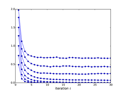
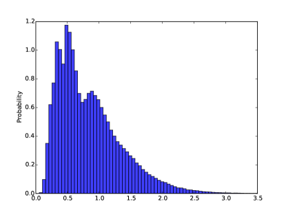
Figure 4: Solution of the recursive distributional equation (210) using the population dynamics algorithm. Left frame: evolution of the mean ${\mathbb{E}}\{{\sf c}^{t}\}$ versus the number of iterations $t$, as estimated by the algorithm. Various curves refer (from bottom to top) to $d=0.5$, $0.75$, $1$, $1.25$, $1.5$, $1.75$, $2$. Here sample size is $N=5\cdot 10^{3}$. Right frame: histogram of the samples at convergence, for $d=2$. Here $N=5\cdot 10^{3}$.

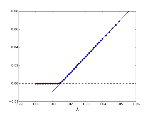
Figure 5: Local stability of the ${\mathcal{O}}(m)$ symetric phase. We evaluate $G_{2}(d,\lambda)$ defined by Eq. (231) using the population dynamics algorithm. Data here reder to average degree $d=6$. The phase transition point $\tilde{\lambda}_{c}^{\mbox{\tiny{SDP}}}(d)$ (within the vectorial ansatz) is determined by a local linear fit to the estimated $G_{2}(d,\lambda)$, when it is significantly larger than $0$.

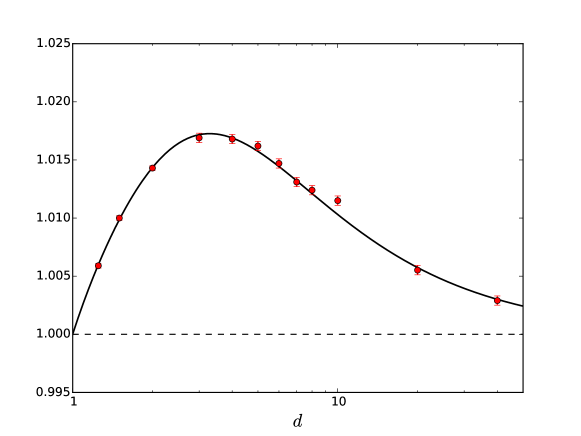
Figure 6: Theoretical prediction of the phase transition location for detecting hidden partition in sparse graphs using semidefinite programming. here the phase transition location is reported in the rescaled variable $\lambda=(a-b)/\sqrt{2(a+b)}$ as a function of the average degree $d=(a+b)/2$. Points with error bars correspond to the definition (232), evaluated numerically by approximating the recursion (230) with the population dynamics algorithm. The continuous curve is a rational fit to the data, constrained at $d=1$, and for large $d$.

We used the obvious modification of this algorithm to implement the recursion (230), whereby a population is now formed of pairs $({\sf c}^{t}_{1},h^{t}_{1})$, …$({\sf c}^{t}_{N},h^{t}_{N})$. An important difference is that the overall scaling of the $h^{t}_{i}$ is immaterial. We hence normalize them at each iteration as follows

$$(h^{t}_{i})^{{\rm new}}=\frac{h^{t}_{i}}{\sqrt{M_{t}}}\,,\;\;\;\;\;M_{t}\equiv\frac{1}{N}\sum_{i=1}^{N}(h^{t}_{i})^{2}\,.$$ (246)

The normalization constant $M_{t}$ also allow us to estimate $G_{2}(d,\lambda)$, namely

$$\widehat{G}_{2}(d,\lambda)\equiv\frac{1}{2(t_{\max}-t_{\min}+1)}\sum_{t=t_{\min}}^{t_{\max}}\log{M_{t}}\,.$$ (247)

Figure 5 presents the typical results of this calculation, using $N=10^{7}$, $t_{\min}=100$, $t_{\max}=400$, at average degree $d=6$.

The behavior in Figure 5 is generic. For small $\lambda$, the estimate $\widehat{G}_{2}(d,\lambda)$ is statistically indistinguishable from $0$. Above a critical point, that we identify with $\tilde{\lambda}_{c}^{\mbox{\tiny{SDP}}}(d)$, $\widehat{G}_{2}(d,\lambda)$ is strictly positive, and essentially linear in $\lambda$, close to $\tilde{\lambda}_{c}^{\mbox{\tiny{SDP}}}(d)$. In order to estimate $\tilde{\lambda}_{c}^{\mbox{\tiny{SDP}}}(d)$ we use a local linear fit, with parameters $g_{0}$, $g_{1}$

$$\widehat{G}_{2}(d,\lambda)=g_{0}+g_{1}\lambda\,,$$ (248)

and set $\tilde{\lambda}_{c}^{\mbox{\tiny{SDP}}}(d)=-\hat{g}_{0}/\hat{g}_{1}$. In the fit we include only the values of $\lambda$ such that $\widehat{G}_{2}(d,\lambda)$ is significantly different from $0$. Note that the linear fit here is in a local neighborhood of $\lambda=1$. By equation (240), it is easy to see that for large fixed $d$, $G_{2}(d,\lambda)$ is logarithmic in $\lambda$.

The resulting values of $\tilde{\lambda}_{c}^{\mbox{\tiny{SDP}}}(d)$ are plotted in Figure 6, together with statistical errors. We report the same values in Table 1 (note that the value for $d=10$ appears to be an outlier).

$d$	$\tilde{\lambda}_{c}^{\mbox{\tiny{SDP}}}(d)$
$1.25$	$1.0059\pm 0.0002$
$1.5$	$1.0100\pm 0.0002$
$2$	$1.0143\pm 0.0002$
$3$	$1.0169\pm 0.0004$
$4$	$1.0168\pm 0.0004$
$5$	$1.0162\pm 0.0004$
$6$	$1.0147\pm 0.0004$
$7$	$1.0131\pm 0.0004$
$8$	$1.0124\pm 0.0004$
$10$	$1.0115\pm 0.0004$
$20$	$1.0055\pm 0.0004$
$40$	$1.0029\pm 0.0004$

Table 1: Numerical determination of the critical point $\tilde{\lambda}_{c}^{\mbox{\tiny{SDP}}}(d)$ (within the vectorial ansatz) for a few values of $d$.

In order to interpolate these results, we fitted a rational function, with the correct asymptotic behavior at $d=1$ (namely, $\tilde{\lambda}_{c}^{\mbox{\tiny{SDP}}}(d=1)=1$) and at $d\to\infty$ (namely, $\tilde{\lambda}_{c}^{\mbox{\tiny{SDP}}}(d)=1+1/(8d)+o(d^{-1})$). This fit is reported as a continuous line in Figure 5, and is given by

$$\lambda^{\mbox{\tiny FIT}}_{c}(d)=1+\frac{a_{1}(d-1)+a_{2}(d-1)^{2}}{1+b_{1}(d-1)+(8a_{1}+19.5a_{2})(d-1)^{2}+8a_{2}(d-1)^{3}}\,,$$ (249)

with parameters

$$a_{1} =0.0307569\,,$$ (250)

$$a_{2} =0.030035\,,$$ (251)

$$b_{1} =2.16454\,.$$ (252)

This is also the curve reported in the main text.

9.4 The recovery phase (broken ${\mathcal{O}}(m)$ symmetry)

In this section we describe an approximate solution of the cavity equations within the region $\lambda>\lambda_{c}^{\mbox{\tiny{SDP}}}(d)$. In this regime the SDP estimator has positive correlation with the ground truth (in the $n\to\infty$ limit). We will work within a generalization of the vectorial ansatz introduced in Section 9.2. Namely, we look for a solution which breaks the ${\mathcal{O}}(m)$ symmetry to ${\mathcal{O}}(m-1)$ along the first direction, as follows. Letting ${\bm{\sigma}}_{i}=(s_{i},{\bm{\tau}}_{i})$, $s_{i}\in{\mathbb{R}}$, ${\bm{\tau}}_{i}\in{\mathbb{R}}^{m-1}$, we adopt the ansatz

$$\nu_{i}({\rm d}{\bm{\sigma}}_{i})\cong\exp\Big{\{}2\beta\sqrt{m{\sf c}_{i}}\,\langle{\bm{z}}_{i},{\bm{\tau}}_{i}\rangle+2\beta mh_{i}\,s_{i}-\beta mr_{i}s_{i}^{2}+O_{m}(1)\Big{\}}\,\delta\Big{(}s_{i}^{2}+\|{\bm{\tau}}_{i}\|_{2}^{2}-1\Big{)}\;{\rm d}^{m}{\bm{\sigma}}_{i}\,,$$ (253)

where we will assume ${\bm{z}}_{i}\sim{\sf N}(0,{\rm I}_{m-1})$. In the following, we let ${\sf P}_{1}={\bm{e}}_{1}{\bm{e}}_{1}^{{\sf T}}$ be the projector along the first direction and ${\sf P}^{\perp}_{1}={\rm I}-{\sf P}_{1}$ denote the orthogonal projector.

Recalling the cavity equations (196), and using the Fourier representation of the delta function, we get

$$\widehat{\nu}_{i}({\bm{\sigma}}_{0}) \cong\int\exp\Big{\{}\beta m\rho-\beta m\big{(}(\rho+r_{i})s_{i}^{2}+\rho\|{\bm{\tau}}_{i}\|_{2}^{2}\big{)}$$ (254)

$$\phantom{AAAAAAAAAAA}+2\beta m\big{(}s_{0}s_{i}+\langle{\bm{\tau}}_{0},{\bm{\tau}}_{i}\rangle\big{)}+2\beta mh_{i}s_{i}+2\beta\sqrt{m{\sf c}_{i}}\langle{\bm{z}}_{i},{\bm{\tau}}_{i}\rangle\Big{\}}\,{\rm d}\rho\,{\rm d}^{m-1}{\bm{\tau}}_{i}{\rm d}s_{i}$$

$$\cong\int\rho^{-m/2}\,\exp\Big{\{}\beta m\rho+\frac{(2\beta ms_{0}+2\beta mh_{i})^{2}}{4\beta m(\rho+r_{i})}\ +\frac{\|2\beta m{\bm{\tau}}_{0}+2\beta\sqrt{m{\sf c}_{i}}{\bm{z}}_{i}\|_{2}^{2}}{4\beta m\rho}\Big{\}}\,{\rm d}\rho$$ (255)

$$\cong\int\exp\Big{\{}\beta mS_{i}(\rho;s_{0})+\frac{2\beta\sqrt{m{\sf c}_{i}}}{\rho}\langle{\bm{z}}_{i},{\bm{\tau}}_{0}\rangle\Big{\}}\,{\rm d}\rho\,,$$ (256)

where

$$S_{i}(\rho;s_{0}) =S_{i,0}(\rho)+S_{i,1}(\rho)\,s_{0}+\frac{1}{2}S_{i,2}(\rho)\,s_{0}^{2}\,,$$ (257)

$$S_{i,0}(\rho) \equiv\rho-\frac{1}{2\beta}\log\rho+\frac{h_{i}^{2}}{\rho+r_{i}}+\frac{1+{\sf c}_{i}}{\rho}\,,$$ (258)

$$S_{i,1}(\rho) =\frac{2h_{i}}{\rho+r_{i}}\,,$$ (259)

$$S_{i,2}(\rho) =\frac{2}{\rho+r_{i}}-\frac{2}{\rho}\,.$$ (260)

where we approximated $\|{\bm{z}}_{i}\|_{2}^{2}/m\approx 1$, and used the identity $\|{\bm{\tau}}_{0}\|_{2}^{2}=1-s_{0}^{2}$. In the $m\to\infty$ limit, we approximate the integral over $\rho$ by its saddle point. In order to obtain a set of equations for the parameters of the ansatz (253), we will expand the exponent to second order in $s_{0}$. The saddle point location is given by

$$\rho_{i,*}(s_{0}) \equiv\arg\min_{\rho\in{\mathbb{R}}_{>0}}S_{i}(\rho;s_{0})=\rho_{i}+\rho_{i,1}s_{0}+O(s_{0}^{2})\,.$$ (261)

Here $\rho_{i}$ solves the equation $S^{\prime}_{i,0}(\rho_{i})=0$. Henceforth we shall focus on the $\beta\to\infty$ limit, in which the equation $S^{\prime}_{i,0}(\rho_{i})=0$ reduces to

$$1=\frac{h_{i}^{2}}{(\rho_{i}+r_{i})^{2}}+\frac{1+{\sf c}_{i}}{\rho_{i}^{2}}\,.$$ (262)

The first order correction is given by $\rho_{i,1}=-S^{\prime}_{i,1}(\rho_{i})/S_{i,0}^{\prime\prime}(\rho_{i})$. Substituting in Eq. (257), we get the saddle point value of $S_{i}(\rho_{i};s_{0})$:

$$\min_{\rho\in{\mathbb{R}}_{>0}}S_{i}(\rho;s_{0}) =S_{i,0}(\rho_{i})+S_{i,1}(\rho_{i})\,s_{0}+\Delta_{2}s_{0}^{2}+O(s_{0}^{3})\,,$$ (263)

$$\Delta_{2} =\frac{1}{2}\left[S_{i,2}(\rho_{i})-\frac{S^{\prime}_{i,1}(\rho_{i})^{2}}{S^{\prime\prime}_{i,0}(\rho_{i})}\right]$$ (264)

$$=-\frac{1}{\rho_{i}}+\frac{1}{\rho_{i}+r_{i}}-\left(\frac{h_{i}^{2}}{(\rho_{i}+r_{i})^{3}}+\frac{1+{\sf c}_{i}}{\rho_{i}^{3}}\right)^{-1}\frac{h_{i}^{2}}{(\rho_{i}+r_{i})^{4}}$$ (265)

$$=-\frac{1}{\rho_{i}}+\frac{1}{\rho_{i}+r_{i}}-\left(1+\frac{(1+{\sf c}_{i})r_{i}}{\rho_{i}^{3}}\right)^{-1}\frac{h_{i}^{2}}{(\rho_{i}+r_{i})^{3}}\,,$$ (266)

where in the last expression we used Eq. (262). Substituting in Eq. (196), we get a recursion for the triple $h_{i}$, ${\sf c}_{i}$, $r_{i}$:

$${\sf c}_{0} =\sum_{i=1}^{k}\frac{{\sf c}_{i}}{\rho_{i}^{2}}\,,$$ (267)

$$h_{0} =\sum_{i=1}^{k}\frac{h_{i}}{\rho_{i}+r_{i}}\,,$$ (268)

$$r_{0} =\sum_{i=1}^{k}\left\{\frac{1}{\rho_{i}}-\frac{1}{\rho_{i}+r_{i}}+\left(1+\frac{(1+{\sf c}_{i})r_{i}}{\rho_{i}^{3}}\right)^{-1}\frac{h_{i}^{2}}{(\rho_{i}+r_{i})^{3}}\right\}$$ (269)

If $G_{n}$ is distributed according to the two-groups stochastic block model, the distributions of this triples on different type vertices are related by symmetry $({\sf c}_{i(+)},h_{i(+)},r_{i(+)})\stackrel{{\scriptstyle{\rm d}}}{{=}}({\sf c}_{i(-)},-h_{i(-)},r_{i(-)})$ for $i(+)\in V_{+}$, $i(-)\in V_{-}$. This leads to the following distributional recursion for the sequence of random vectors $\{({\sf c}^{t},h^{t},r^{t})\}_{t\geq 0}$:

$${\sf c}^{t+1} =\sum_{i=1}^{L_{+}+L_{-}}\frac{{\sf c}^{t}_{i}}{\rho_{i}^{2}}\,,$$ (270)

$$h^{t+1} =\sum_{i=1}^{L_{+}+L_{-}}\frac{s_{i}h^{t}_{i}}{\rho_{i}+r^{t}_{i}}\,,$$ (271)

$$r^{t+1} =\sum_{i=1}^{L_{+}+L_{-}}\left\{\frac{1}{\rho_{i}}-\frac{1}{\rho_{i}+r^{t}_{i}}+\left(1+\frac{(1+{\sf c}^{t}_{i})r^{t}_{i}}{\rho_{i}^{3}}\right)^{-1}\frac{(h^{t}_{i})^{2}}{(\rho_{i}+r^{t}_{i})^{3}}\right\}\,,$$ (272)

where $L_{+}\sim{\rm Poisson}(a/2)$, $L_{-}\sim{\rm Poisson}(b/2)$, $s_{1},\dots,s_{L_{+}}=+1$, $s_{L_{+}+1},\dots,s_{L_{+}+L_{-}}=-1$, and $\{({\sf c}_{i}^{t},h^{t}_{i},r^{t}_{i})\}$ are i.i.d. copies of $({\sf c}^{t},h^{t},r^{t})$. Finally, $\rho_{i}$ is a function of $({\sf c}_{i}^{t},h^{t}_{i},r^{t}_{i})$ implicitly defined as the solution of

$$1=\frac{(h^{t}_{i})^{2}}{(\rho_{i}+r^{t}_{i})^{2}}+\frac{1+{\sf c}^{t}_{i}}{\rho_{i}^{2}}\,.$$ (273)

As a check of the above derivation, we next verify that we recover the correct $d\to\infty$ limit, captured by the ${\mathbb{Z}}_{2}$ synchronization model, cf. Section 7.2.5. We will focus on the fixed point of recursions (270) to (272), and hence omit iteration index $t$. For large degree, we expect central limit theorem to imply the following asymptotic behaviors:

$${\sf c}_{i} =d\,\mu_{{\sf c}}+O(\sqrt{d})\,,$$ (274)

$$h_{i} \stackrel{{\scriptstyle{\rm d}}}{{=}}\sqrt{d}\big{(}\mu_{h}+\sigma_{h}\,Z\big{)}+o(\sqrt{d})\,,$$ (275)

$$r_{i} =\sqrt{d}\,\mu_{r}+O(1)\,,$$ (276)

where $\mu_{{\sf c}}$, $\mu_{h}$, $\sigma_{h}$, $\mu_{r}$ are deterministic parameters to be determined. Equation (273) thus implies $\rho_{i}=\sqrt{d}\rho$, with $\rho$ solution of

$$1=\frac{(\mu_{h}+\sigma_{h}Z)^{2}}{(\rho+\mu_{r})^{2}}+\frac{\mu_{{\sf c}}}{\rho^{2}}\,.$$ (277)

Equations (270) to (272) then yield the following. From Eq.  (270) we get

$$\mu_{{\sf c}} =\mu_{{\sf c}}{\mathbb{E}}\left\{\frac{1}{\rho^{2}}\right\}\,,$$ (278)

i.e., assuming $\mu_{{\sf c}}\neq 0$, ${\mathbb{E}}\{\rho^{-2}\}=1$. From Eq.  (271) we get

$$\mu_{h} =\lambda\,{\mathbb{E}}\left\{\left(\frac{\mu_{h}+\sigma_{h}Z}{\rho+\mu_{r}}\right)\right\}\,,$$ (279)

$$\sigma_{h}^{2} ={\mathbb{E}}\left\{\left(\frac{\mu_{h}+\sigma_{h}Z}{\rho+\mu_{r}}\right)^{2}\right\}\,.$$ (280)

Finally, from Eq. (272) we get

$$\mu_{r} ={\mathbb{E}}\left\{\frac{1}{\rho}-\frac{1}{\rho+\mu_{r}}+\left(1+\frac{\mu_{{\sf c}}\mu_{r}}{\rho^{3}}\right)^{-1}\frac{(\mu_{h}+\sigma_{h}Z)^{2}}{(\rho+\mu_{r})^{3}}\right\}\,.$$ (281)

We claim that these equations are equivalent to the ones for the ${\mathbb{Z}}_{2}$ synchronization problem, derived using the replica method, namely Eqs. (125) to (128). Indeed Eq. (128) coincides with Eq. (278), for $\mu_{{\sf c}}\neq 0$. Setting $\mu_{h}=\mu$, $\sigma_{h}^{2}=q$, and $\mu_{r}=r$, we obtain that Eqs. (125), (126) coincide with Eqs. (279), (280). Further, taking expectation of Eq. (277), and using ${\mathbb{E}}\{\rho^{-2}\}=1$, we get $\mu_{\sf c}=1-q$. Hence, we obtain that Eq. (277) coincides with Eq. (124).

Substituting the values of various parameters in Eq. (281), we obtain

$$r ={\mathbb{E}}\left\{\frac{1}{\rho}-\frac{1}{\rho+r}+\left(1+\frac{r(1-q)}{\rho^{3}}\right)^{-1}\frac{(\mu+\sqrt{q}Z)^{2}}{(\rho+r)^{3}}\right\}\,.$$ (282)

We claim that this is equivalent to Eq. (127). To see this, notice that differentiating Eq. (277) with respect to $Z$ we get

$$\frac{\partial\rho}{\partial Z} =\left[\frac{(\mu+\sqrt{q}Z)^{2}}{(\rho+r)^{3}}+\frac{(1-q)}{\rho^{3}}\right]^{-1}\cdot\frac{(\mu+\sqrt{q}Z)\sqrt{q}}{(\rho+r)^{2}}$$ (283)

$$=\left(1+\frac{r(1-q)}{\rho^{3}}\right)^{-1}\frac{(\mu+\sqrt{q}Z)\sqrt{q}}{\rho+r}\,,$$ (284)

where the second equality follows again from Eq. (277). Using this identity, we can rewrite Eq. (282) as

$$r ={\mathbb{E}}\left\{\frac{1}{\rho}-\frac{1}{\rho+r}+\frac{1}{\sqrt{q}}\frac{(\mu+\sqrt{q}Z)}{(\rho+r)^{2}}\,\frac{\partial\rho}{\partial Z}\right\}\,,$$ (285)

or

$$r ={\mathbb{E}}\left\{\frac{1}{\rho}-\frac{1}{\sqrt{q}}\frac{\partial\phantom{Z}}{\partial Z}\frac{\mu+\sqrt{q}Z}{\rho+r}\right\}\,,$$ (286)

Using Gaussian integration by parts in the second term we finally obtain Eq. (127). This concludes our verification for the case of $d\to\infty$.

9.5 Limitations of the vectorial ansatz

Our analytical estimate of the SDP phase transition location, $\tilde{\lambda}_{c}^{\mbox{\tiny{SDP}}}(d)$ was carried out within the vectorial ansatz in Eqs. (198), (224). Let us stress once again that this ansatz is only approximate.

The origin of this approximation can be gleaned from the calculation in Section 9.1. As we have seen Eq. (206) is only accurate when $\langle{\bm{\sigma}}_{0},{\bm{z}}_{i}\rangle$ is small. However, according to the same ansatz, ${\bm{\sigma}}_{0}$ will be aligned to ${\bm{z}}_{0}$, which –in turn– can be aligned with ${\bm{z}}_{i}$.

We expect this approximation to be accurate in the following regimes:

• For large average degree $d$. Indeed, in this case, ${\bm{z}}_{0}$ is weakly correlated with ${\bm{z}}_{i}$.

• For $d$ close to $1$. In this case ${\sf c}_{0}$ is small and hence, under $\nu_{0}$, ${\bm{\sigma}}_{0}$ is approximately uniformly distributed, and hence has a small scalar product $\langle{\bm{z}}_{i},{\bm{\sigma}}_{0}\rangle$.

Let us also notice that the vectorial ansatz can be systematically improved upon by considering quadratic terms tepending in two-dimensional projections, and so on. We leave this direction for future work.

10 Numerical experiments for community detection

In this section we provide details about our numerical simulations with the SDP estimator for the community detection problem. For the reader’s convenience we begin by recalling some definitions.

We denote by $G_{n}=(V_{n},E_{n})$ the random graph over vertex set $V_{n}=[n]$, generated according the hidden partition model, and by $\bm{x_{0}}\in\{+1,-1\}^{n}$ the vertex labels. Conditional on $\bm{x_{0}}$, edges are independent with distribution

$${\mathbb{P}}\big{\{}(i,j)\in E_{n}\big{|}\bm{x_{0}}\big{\}}=\begin{cases}a/n&\mbox{ if $x_{0,i}x_{0,j}=+1$,}\\ b/n&\mbox{ if $x_{0,i}x_{0,j}=-1$.}\end{cases}$$ (287)

We denote by $d=(a+b)/2$ the average degree, and by $\lambda=(a-b)/\sqrt{2(a+b)}$ the ‘signal strength.’

Throughout this section, ${\partial i}$ indicates the set of neighbors of vertex $i$, i.e. ${\partial i}\equiv\{j\in[n]:(i,j)\in E\}$.

We next recall the SDP relaxation for estimating community memberships:

$$\begin{split}\mbox{maximize}&\;\;\;\sum_{(i,j)\in E}X_{ij}\,,\\ \mbox{subject to}&\;\;\;\bm{X}\succeq 0\,,\\ &\;\;\;\bm{X}{\mathbf{1}}={\mathbf{0}}\,,\;\;\;\;X_{ii}=1\;\;\forall i\in[n]\,.\end{split}$$ (288)

Denote by $\bm{X}_{\mbox{\tiny{opt}}}=\bm{X}_{\mbox{\tiny{opt}}}(G)$ an optimizer of the above problem. The estimated membership vector is then obtained by ‘rounding’ the principal eigenvector of $\bm{X}_{\mbox{\tiny{opt}}}$ as follows. Letting ${\bm{v}}_{1}={\bm{v}}_{1}(\bm{X}_{\mbox{\tiny{opt}}})$ be the principle eigenvector of $\bm{X}_{\mbox{\tiny{opt}}}$, the SDP estimate is given by

$$\bm{\hat{x}}^{\mbox{\tiny{SDP}}}(G)={\rm sign}\big{(}{\bm{v}}_{1}(\bm{X}_{\mbox{\tiny{opt}}}(G))\big{)}\,.$$ (289)

We measure the performance of such an estimator via the overlap:

$${\rm Overlap}_{n}(\bm{\hat{x}}^{\mbox{\tiny{SDP}}})=\frac{1}{n}{\mathbb{E}}\big{\{}\big{|}\langle\bm{\hat{x}}^{\mbox{\tiny{SDP}}}(G),\bm{x_{0}}\rangle\big{|}\big{\}}\,,$$ (290)

where $\bm{x_{0}}\in\{-1,+1\}^{n}$ encodes the ground truth memberships with $x_{0,i}=+1$ if $i\in V_{+}$ and $x_{0,i}=-1$ if $i\in V_{-}$. Note that ${\rm Overlap}_{n}(\bm{\hat{x}}^{\mbox{\tiny{SDP}}})\in[0,1]$ and a random guessing estimator yields overlap of order $O(1/\sqrt{n})$.

The majority of our calculations were run on a cluster with $160$ cores (Intel Xeon), taking roughly a month (hence total CPU time was roughly 10 years).

10.1 Optimization algorithms

We write SDP optimization (288) in terms of the vector spin model. Let ${\bm{\sigma}}_{i}\in{\mathbb{R}}^{m}$ be the vector spin assigned to node $i$, for $i\in[n]$, and define ${\bm{\sigma}}\equiv({\bm{\sigma}}_{1},{\bm{\sigma}}_{2},\dotsc,{\bm{\sigma}}_{n})$. We then rewrite the SDP (288) as

$$\begin{split}\underset{{\underline{{\bm{\sigma}}}}}{\mbox{maximize}}&\;\;\;F({\bm{\sigma}})\equiv\sum_{(i,j)\in E}\langle{\bm{\sigma}}_{i},{\bm{\sigma}}_{j}\rangle\,,\\ \mbox{subject to}&\;\;\;{\bm{\sigma}}\in{\cal M}(n,m)\,,\end{split}$$ (291)

where the manifold ${\cal M}(n,m)$ is defined as below:

$${\cal M}(n,m)=\Big{\{}{\bm{\sigma}}=({\bm{\sigma}}_{1},\dots,{\bm{\sigma}}_{n})\in({\mathbb{R}}^{m})^{n}:\;\|{\bm{\sigma}}_{i}\|_{2}=1\,,\;\;\sum_{i=1}^{n}{\bm{\sigma}}_{i}=0\Big{\}}\,.$$ (292)

We will omit the dimensions when they are clear from the context.

As discussed in the main text, the two optimization problems (288) and (291) have a value that differ by a relative error of $O(1/m)$, uniformly in the size $n$. In particular, the asymptotic value of the SDP is the same, if we let $m\to\infty$ after $n\to\infty$.

In fact the following empirical findings (further discussed below) point at a much stronger connection:

1. With high probability, the optimizer appears to be essentially independent of $m$ already for moderate values of $m$ (in practice, already for $m=40\sim 100$, when $n\lesssim 10^{4}$).

2. Again, for moderate values of $m$, optimization methods do not appear to be stuck in local minima. Roughly speaking, while the problem is non-convex from a worst case perspective, typical instances are nearly convex.

Motivated by these findings, we solve optimization problem (291) in lieu of SDP problem (288), using the two algorithms described below: $(i)$ Projected gradient ascent; $(ii)$ Block-coordinate ascent.

The rank-constrained formulation also allows to accelerate the rounding step to compute $\bm{\hat{x}}^{\mbox{\tiny{SDP}}}(G)$, which can be obtained in time $O(nm^{2}+m^{3})$, instead of the naive $O(n^{3})$. Namely, given an optimizer ${\bm{\sigma}}^{\mbox{\tiny{opt}}}$, we compute the $m\times m$ empirical covariance matrix

$${\bf\widehat{\Sigma}}\equiv\frac{1}{n}\sum_{i=1}^{n}{\bm{\sigma}}_{i}^{\mbox{\tiny{opt}}}({\bm{\sigma}}_{i}^{\mbox{\tiny{opt}}})^{\sf T}\,.$$ (293)

Denoting by ${\bm{\varphi}}$ the principal eigenvector of ${\bf\widehat{\Sigma}}$, we obtain the estimator $\bm{\hat{x}}^{\mbox{\tiny{SDP}}}(G)\in\{1,-1\}^{n}$ via

$$\hat{x}^{\mbox{\tiny{SDP}}}_{i}={\rm sign}\big{(}\langle{\bm{\varphi}},{\bm{\sigma}}^{\mbox{\tiny{opt}}}_{i}\rangle\big{)}\,.$$ (294)

This approach allows us to carry out high-precision simulations for large instances, namely up to $n=64,000$. By comparison, standard SDP solvers are based on interior-point methods and cannot scale beyond $n$ of the order of a few hundreds.

10.1.1 Projected gradient ascent

The tangent space at ${\bm{\sigma}}\in{\cal M}$ is given by

$${\sf T}_{{\bm{\sigma}}}{\cal M}\simeq\Big{\{}{\bm{z}}=({\bm{z}}_{1},\dots,{\bm{z}}_{n}):\,\langle{\bm{\sigma}}_{i},{\bm{z}}_{i}\rangle=0\,,\;\sum_{i=1}^{n}{\bm{z}}_{i}=0\Big{\}}\,.$$ (295)

Define the orthogonal projectors in ${\mathbb{R}}^{m}$:

$${\sf P}_{i}\equiv{\bm{\sigma}}_{i}{\bm{\sigma}}_{i}^{{\sf T}}\,,\;\;\;{\sf P}^{\perp}_{i}\equiv{\rm I}-{\bm{\sigma}}_{i}{\bm{\sigma}}_{i}^{{\sf T}}\,.$$ (296)

By identification (295), the manifold gradient of $F$ reads

$$\begin{split}\nabla F({\bm{\sigma}})&=\big{(}\nabla F({\bm{\sigma}})_{1},\dots,\nabla F({\bm{\sigma}})_{n}\big{)}\,,\\ \nabla F({\bm{\sigma}})_{i}&={\sf P}^{\perp}_{i}({\bm{v}}_{i}-{\bm{\overline{v}}}_{i})\,,\end{split}$$ (297)

where

$$\begin{split}{\bm{v}}_{i}({\bm{\sigma}})&\equiv\sum_{j\in{\partial i}}{\bm{\sigma}}_{j}\,,\\ {\bm{\overline{v}}}&\equiv\Big{(}\sum_{i=1}^{n}{\sf P}^{\perp}_{i}\Big{)}^{-1}\Big{(}\sum_{i=1}^{n}{\sf P}^{\perp}_{i}{\bm{v}}_{i}\Big{)}\,.\end{split}$$ (298)

We next define the convex envelope of ${\cal M}$:

$${\rm conv}({\cal M})=\Big{\{}{\bm{\sigma}}=({\bm{\sigma}}_{1},\dots,{\bm{\sigma}}_{n})\in({\mathbb{R}}^{m})^{n}:\;\|{\bm{\sigma}}_{i}\|\leq 1\,,\;\;\sum_{i=1}^{n}{\bm{\sigma}}_{i}=0\Big{\}}\,,$$ (299)

and the corresponding orthogonal projector

$${\sf P}_{{\cal M}}({\bm{y}})\equiv\arg\min_{{\bm{z}}\in{\rm conv}({\cal M})}\|{\bm{y}}-{\bm{z}}\|_{2}\,.$$ (300)

The projected gradient method alternates between a step in the direction of $\nabla F({\bm{\sigma}})$ and a projection onto ${\rm conv}({\cal M})$. Pseudocode is given as Algorithm 2.

Algorithm 2 Projected gradient ascent for relaxed min bisection

0:  $n$,$m$, edge set $E\subseteq[n]\times[n]$, ${\tt tol}_{2}$

0:  ${\bm{\sigma}}^{\mbox{\tiny{opt}}}\equiv({\bm{\sigma}}_{1}^{\mbox{\tiny{opt}}},\dotsc,{\bm{\sigma}}_{n}^{\mbox{\tiny{opt}}})$

1:  Initialize ${\bm{\sigma}}^{0}\in{\cal M}$ at random(e.g. by letting ${\bm{\sigma}}_{i}\in\{\pm{\bm{e}}_{1},\pm{\bm{e}}_{2},\dotsc,\pm{\bm{e}}_{m}\}$ uniformly random conditional on $\sum_{i=1}^{n}{\bm{\sigma}}_{i}^{0}=0$).

2:  for  $t=0,1,2,\dots$ do

3:     Gradient step

$$\bm{\tilde{{\bm{\sigma}}}}^{t+1}={\bm{\sigma}}^{t}+{\varepsilon}_{t}\nabla F({\bm{\sigma}}^{t})\,,$$ (301)

with ${\varepsilon}_{t}=1/\sqrt{t}$ the step size.

4:     Projection step:

$${\bm{\sigma}}^{t+1}={\sf P}_{{\cal M}}(\bm{\tilde{{\bm{\sigma}}}}^{t+1})\,.$$ (302)

5:     if $\|\nabla F({\bm{\sigma}}^{t+1})\|_{2}/\sqrt{n}\leq{\tt tol}_{2}$ then

6:        set $T=t$

7:        break

8:  return  ${\bm{\sigma}}^{\mbox{\tiny{opt}}}={\bm{\sigma}}^{t}$

The projected gradient method requires a subroutine for computing the projection ${\sf P}_{{\cal M}}$ onto ${\rm conv}({\cal M})$. In order to compute this projection, we write the Lagrangian corresponding to problem (300):

$$\mathcal{L}\equiv\frac{1}{2}\sum_{i=1}^{n}\|{\bm{y}}_{i}-{\bm{z}}_{i}\|_{2}^{2}+{\bm{w}}^{\sf T}\sum_{i=1}^{n}{\bm{z}}_{i}+\sum_{i=1}^{n}\frac{\mu_{i}}{2}(\|{\bm{z}}_{i}\|_{2}^{2}-1)\,,$$ (303)

with $\mu\geq 0$ for $1\leq i\leq n$. Setting $\nabla_{{\bm{z}}_{i}}\mathcal{L}=0$, we obtain

$${\bm{z}}_{i}=\frac{{\bm{y}}_{i}-{\bm{w}}}{\mu_{i}+1}\,.$$ (304)

Further, the constraint $\sum_{i=1}^{n}{\bm{z}}_{i}=0$ implies

$${\bm{w}}=\Big{(}\sum_{i=1}^{n}\frac{1}{\mu_{i}+1}\Big{)}^{-1}\Big{(}\sum_{i=1}^{n}\frac{{\bm{y}}_{i}}{\mu_{i}+1}\Big{)}\,.$$ (305)

Due to constraint $\|{\bm{z}}_{i}\|\leq 1$, we have $\mu_{i}\geq\|{\bm{y}}_{i}-{\bm{w}}\|-1$. Also, by the KKT conditions, if the inequality is strict we have $\mu_{i}=0$. Therefore,

$$\mu_{i}=\max(\|{\bm{y}}_{i}-{\bm{w}}\|_{2}-1,0)\,.$$ (306)

Substituting for $\mu_{i}$ from Eq. (306) into (305) we arrive at

$${\bm{w}}=\Big{(}\sum_{i=1}^{n}\frac{1}{\max(\|{\bm{y}}_{i}-{\bm{w}}\|_{2},1)}\Big{)}^{-1}\Big{(}\sum_{i=1}^{n}\frac{{\bm{y}}_{i}}{\max(|{\bm{y}}_{i}-{\bm{w}}\|,1)}\Big{)}\,.$$ (307)

We compute the Lagrange multiplier ${\bm{w}}$ in an iterative manner as described in Algorithm 3.

Algorithm 3 Algorithm for computing the projection ${\sf P}_{{\cal M}}({\bm{y}})$

0:  ${\bm{y}}$, ${\tt tol}_{1}$

0:  ${\sf P}_{{\cal M}}({\bm{y}})$

1:  ${\bm{w}}^{0}\leftarrow\mathbf{0}$

2:  for  $t=0,1,2,\dots$ do

3:     update

$${\bm{w}}^{t+1}=\Big{(}\sum_{i=1}^{n}\frac{1}{\max(\|{\bm{y}}_{i}-{\bm{w}}^{t}\|_{2},1)}\Big{)}^{-1}\Big{(}\sum_{i=1}^{n}\frac{{\bm{y}}_{i}}{\max(\|{\bm{y}}_{i}-{\bm{w}}^{t}\|_{2},1)}\Big{)}\,.$$ (308)

4:     if $\|{\bm{w}}^{t+1}-{\bm{w}}^{t}\|_{2}\leq{\tt tol}_{1}$ then

5:        set $T=t$

6:        break

7:  return  

$${\sf P}_{{\cal M}}({\bm{y}})_{i}=\frac{{\bm{y}}_{i}-{\bm{w}}^{T}}{\max(\|{\bm{y}}_{i}-{\bm{w}}^{T}\|,1)}\,,\quad\quad{\rm for}\quad i=\{1,2,\dotsc,n\}\,.$$ (309)

10.1.2 Block coordinate ascent

We present here a second algorithm to solve problem (291), that uses block-coordinate descent. This provides independent check of numerical results. Further, this second method appears to be faster than projected gradient ascent.

We start by considering an unconstrained version of the optimization problem (with $\bm{A}_{G}$ the adjacency matrix of the graph $G$):

maximize $$\langle{\bm{\sigma}},\big{(}\bm{A}_{G}-\eta{\mathbf{1}}{\mathbf{1}}^{{\sf T}}\big{)}{\bm{\sigma}}\rangle\,.$$ (310)

Equivalently, this objective function can be written as $F({\underline{{\bm{\sigma}}}})-\eta\|{\bm{M}}({\bm{\sigma}})\|^{2}_{2}/2$, where ${\bm{M}}({\bm{\sigma}})\equiv\sum_{i=1}^{n}{\bm{\sigma}}_{i}$. As $\eta\to\infty$, this is of course equivalent to problem (291).

For $G$ distributed according to the hidden partition model (287), with random vertex labels $\bm{x_{0}}$, we have ${\mathbb{E}}\{(\bm{A}_{G})_{ij}\}=d/n$. This suggests that $\eta\geq d/n$ should be sufficient to obtain a balanced partition. In practice we will take $\eta\approx 1$ and check that this yields well balanced partitions (i.e. ${\bm{M}}\approx 0$), cf. Section 10.3.1 below.

We maximize the objective by iteratively maximizing over each of the vectors ${\bm{\sigma}}_{i}$. The latter optimization has a close form expression. More precisely, at each step of this dynamics, we sort the variables in a random order and we update them sequentially, by maximizing the objective function. This is easily done by aligning ${\bm{\sigma}}_{i}$ along the ‘local field’

$$\bm{h}_{i}\equiv-\eta\,{\bm{M}}({\underline{{\bm{\sigma}}}})+\sum_{j:(i,j)\in E}{\bm{\sigma}}_{j}\,.$$ (311)

We check the convergence by measuring the largest variation in a spin variable during the last iteration. Namely we define

$$\Delta_{\text{max}}(t)= \max_{i\in[n]}\|{\bm{\sigma}}_{i}^{t+1}-{\bm{\sigma}}_{i}^{t}\|_{2}\,,$$ (312)

and we use as convergence criterion $\Delta_{\text{max}}<{\tt tol}_{3}$. The corresponding pseudocode is presented as Algorithm 4.

The resulting algorithm is very simple and depends on two parameters ($\eta$ and ${\tt tol}_{3}$) that will be discussed in the Section 10.3, together with dependence on the number $m$ of spin components.

Algorithm 4 Block coordinate ascent for relaxed min bisection

0:  $n$, $m$, edge set $E\subseteq[n]\times[n]$, $\eta$, ${\tt tol}_{3}$

0:  ${\underline{{\bm{\sigma}}}}^{\mbox{\tiny{opt}}}\equiv({\bm{\sigma}}_{1}^{\mbox{\tiny{opt}}},\dotsc,{\bm{\sigma}}_{n}^{\mbox{\tiny{opt}}})$

1:  Initialize ${\underline{{\bm{\sigma}}}}^{0}\in{\cal M}$ at random(e.g. by letting ${\bm{\sigma}}_{i}\in\{\pm{\bm{e}}_{1},\pm{\bm{e}}_{2},\dotsc,\pm{\bm{e}}_{m}\}$ at random so that $\sum_{i}{\bm{\sigma}}_{i}^{0}=0$).

2:  for  $t=1,2,\dots$ do

3:     Choose a random permutation $\pi:[n]\to[n]$

4:     for  $i=1,2,\dots,n$ do

5:        Update spins, aligning to the local field

$${\bm{\sigma}}^{t+1}_{\pi(i)}=\frac{-\eta\,{\bm{M}}({\bm{\sigma}}^{t})+\sum_{j:(\pi(i),j)\in E}{\bm{\sigma}}^{t}_{j}}{\|-\eta\,{\bm{M}}({\bm{\sigma}}^{t})+\sum_{j:(\pi(i),j)\in E}{\bm{\sigma}}^{t}_{j}\|_{2}}\,,$$ (313)

6:     if $\Delta_{\text{max}}(t)\leq{\tt tol}_{3}$ then

7:        set $T=t$

8:        break

9:  return  ${\bm{\sigma}}^{\mbox{\tiny{opt}}}={\bm{\sigma}}^{T}$

10.2 Numerical experiments with the projected gradient ascent

In this section we report our results with the projected gradient algorithm. As mentioned above, we found that the block coordinate ascent method was somewhat faster, and therefore we used the latter for large-statistics simulations, and high-precision determinations of the critical point $\lambda_{c}^{\mbox{\tiny{SDP}}}(d)$. We defer to the next section for further discussion.

We use the projected gradient ascent discussed in Section 10.1.1, with ${\tt tol}_{1}={\tt tol}_{2}=10^{-6}$. For each value of $d\in\{5,10,15,20,25,30\}$ and $n\in\{2000$, $4000$, $8000$, $16000\}$, we generate $500$ realizations of graph $G$ from the stochastic block model defined in Eq. (287). In these experiments, we observed that the estimated membership vector does not change for $m\geq 40$, cf. Section 10.2.1. The results reported here correspond to $m=40$.

Figure 7 reports the estimated overlap ${\rm Overlap}_{n}(\bm{\hat{x}}^{\mbox{\tiny{SDP}}})$ (across realizations) achieved by the SDP estimator, for different values of $d$ and $n$. The solid curve corresponds to the cavity prediction, cf. equation (130), for large $d$. As we see the empirical results are in good agreement with the analytical curve even for small average degrees $d=5,10$.

In particular, the phase transition location seems indistinguishable, on this scale, from $(a-b)/\sqrt{2(a+b)}=1$.

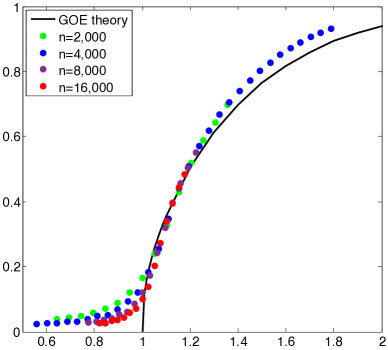
(a) $d=5$

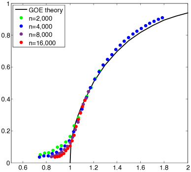
(b) $d=10$

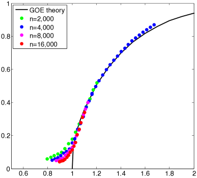
(c) $d=15$

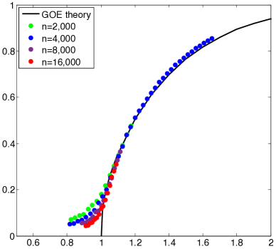
(d) $d=20$

(e) $d=25$

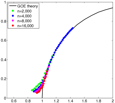
(f) $d=30$

Figure 7: Community detection under the hidden partition model of Eq. (287), for several average degree $d=(a+b)/2$. Dots corresponds to the performance of the SDP reconstruction method (averaged over $500$ realizations). The continuous curve is the asymptotic analytical prediction for the Gaussian model (which captures the large-degree behavior).

10.2.1 Dependence on $m$

As we explained before, optimization problem (291) and SDP (288) are equivalent provided $m\geq n$. In principle, one can solve (291) applying Algorithm 2 with $m=n$. However, this choice leads to a computationally expensive procedure. On the other hand, we expect the solution to be essentially independent of $m$ already for moderate values of $m$. Several theoretical arguments point to this (in particular, the Grothendieck-type inequality of [MS15]). We provide numerical evidence in this section (supporting in particular the choice $m=40$).

In the first experiment, we set the average degree $d=(a+b)/2=5$, $n=4000$ and vary $\lambda=(a-b)/\sqrt{2(a+b)}\in\{0.9,1,1.1,1.2\}$. For each $\lambda$, we solve for $a$ and $b$ and generate $100$ realizations of the graph as per model (287) with parameters $a,b$. For several values of $m$, we solve optimization (291) and report the average overlap and its standard deviation. The results are summarized in Table 2. As we see, for $m\geq 40$ the changes in average overlaps are comparable with the corresponding standard deviations. An interesting observation is that error bars for smaller $m$ are larger, indicating more variations of overlaps across different realizations.

Table 3 demonstrates the results for an analogous experiment with $d=10$.

We observe a similar trend for other several values of $a,b,n$. Based on these observations, we use $m=40$ in our numerical experiments throughout this section.

	$\lambda=0.9$	$\lambda=1$	$\lambda=1.1$	$\lambda=1.2$
$m=5$	$0.1231\pm 0.0037$	$0.0898\pm 0.0059$	$0.2637\pm 0.0074$	$0.4627\pm 0.0017$
$m=10$	$0.1544\pm 0.0008$	$0.0659\pm 0.0045$	$0.3303\pm 0.0018$	$0.4612\pm 0.0006$
$m=20$	$0.1663\pm 0.0002$	$0.1363\pm 0.0008$	$0.3358\pm 0.0005$	$0.4598\pm 0.0002$
$m=40$	$0.1668\pm 0.0001$	$0.1398\pm 0.0002$	$0.3358\pm 0.0002$	$0.4599\pm 0.0001$
$m=80$	$0.1669\pm 0.0001$	$0.1397\pm 0.0002$	$0.3358\pm 0.0002$	$0.4596\pm 0.0001$
$m=160$	$0.1669\pm 0.0001$	$0.1397\pm 0.0002$	$0.3358\pm 0.0002$	$0.4596\pm 0.0001$

Table 2: We fix $d=(a+b)/2=5$ and vary $\lambda=(a-b)/\sqrt{2(a+b)}\in\{0.9,1,1.1.,1.2\}$. The reported values are the average overlaps (over 100 realizations) with one standard deviations, for several values of $m$. As we see for $m\geq 40$, the changes in the average overlaps are comparable to the corresponding standard deviations.

	$\lambda=0.9$	$\lambda=1$	$\lambda=1.1$	$\lambda=1.2$
$m=5$	$0.0875\pm 0.0035$	$0.1385\pm 0.0072$	$0.3760\pm 0.0021$	$0.5045\pm 0.0008$
$m=10$	$0.1322\pm 0.0007$	$0.1943\pm 0.0014$	$0.3873\pm 0.0006$	$0.5050\pm 0.0003$
$m=20$	$0.1346\pm 0.0002$	$0.2100\pm 0.0003$	$0.3890\pm 0.0001$	$0.5070\pm 0.0001$
$m=40$	$0.1353\pm 0.0001$	$0.2089\pm 0.0001$	$0.3885\pm 0.0001$	$0.5088\pm 0.0001$
$m=80$	$0.1354\pm 0.0000$	$0.2090\pm 0.0000$	$0.3885\pm 0.0000$	$0.5089\pm 0.0000$
$m=160$	$0.1354\pm 0.0000$	$0.2090\pm 0.0000$	$0.3885\pm 0.0000$	$0.5089\pm 0.0000$

Table 3: We fix $d=(a+b)/2=10$ and vary $\lambda=(a-b)/\sqrt{2(a+b)}\in\{0.9,1,1.1.,1.2\}$. The reported values are the average overlaps (over 100 realizations) with one standard deviations, for several values of $m$. As we see for $m\geq 40$, the changes in the average overlaps are comparable to the corresponding standard deviations.

10.2.2 Robustness and comparison with spectral methods

Spectral methods are among the most popular nonparametric approaches to clustering. These methods classify nodes according to a the eigenvectors of a matrix associated with the graph, for instance its adjacency matrix or Laplacian. While standard spectral clustering works well when the graph is sufficiently dense or is regular, it is significantly suboptimal for sparse graphs. The reason is that the leading eigenvector of the adjacency matrix is localized around the high degree nodes.

Recently, [KMM⁺13] proposed a class of very interesting spectral methods based on the non-backtracking walk on the directed edges of the graph $G$. The spectrum of non-backtracking matrix is more robust to high-degree nodes because a walk starting at a node cannot return to it immediately. Later, [SKZ14] proposed another spectral method, based on the Bethe Hessian operator, that is computationally more efficient than the non-backtracking operator. Further, the (determinant of the) Bethe Hessian is closely related to the spectrum of the non-backtracking operator and exhibits the same convenient properties for the aim of clustering. Rigorous analysis of spectral methods under the model (287) was carried out in [Mas14, MNS13, BLM15]. The main result of these papers is that spectral methods allow to estimate the hidden partition significantly better than random guessing immediately above the ideal threshold $\lambda=(a-b)/\sqrt{2(a+b)}=1$.

As we saw in the previous section, the threshold of the SDP-based method is extremely close to the ideal one. Here, we compare the Bethe Hessian algorithm with SDP approach in terms of robustness to model miss-specification. We perturb the hidden partition model (287) as follows. For a perturbation level $\alpha\in[0,1]$, we draw $n\alpha$ vertices $i_{1},i_{2},\dotsc,i_{n\alpha}$ uniformly at random and for each vertex $i_{\ell}$, we add to graph $G$ connecting all of the neighbors of $i_{\ell}$. This results in adding $O(nd^{2}\alpha)$ edges to the underlying model (287). This perturbation mimics an important feature of real networks that is absent from the stochastic block model (287), the so-called triangle closure property [EK10] (two friends of a person are often friends).

For perturbation levels $\alpha\in\{0,0.025,0.05\}$, we compare the performance of SDP and Bethe Hessian algorithms in terms of Overlap, defined by (290). Figure 8 summarizes the results for $n=16,000$ and average degree $d=(a+b)/2=10$. The reported overlaps are averaged over $100$ realizations of the model.

In absence of any perturbation (curves $\alpha=0$), the two algorithms have nearly equivalent performances. However, already for $\alpha=0.025$, SDP is substantially superior. While SDP appears to be rather insensitive to the perturbation, the performance of the Bethe Hessian algorithm is severely degraded by it. This is because the added triangles perturb the spectrum of the non-backtracking operator (and similarly of the Bethe Hessian operator) significantly, resulting in poor classification of the nodes.

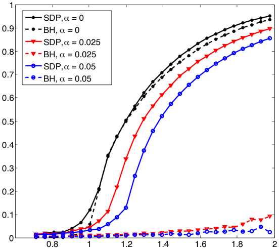
Figure 8: Comparison of SDP and Bethe Hessian algorithm on perturbed hidden partition model. Here, $n=16,000$, $d=(a+b)/2=10$ and we report average overlaps over $100$ realizations. Different colors (markers) represent different perturbation levels $\alpha$. Solid curves are for SDP algorithm and dashed curves are for Bethe-Hessian algorithm. As we see SDP algorithm is more robust than Bethe-Hessian algorithm to the perturbation level $\alpha$.

10.3 Numerical experiments with block coordinate ascent

In this section we present our simulations with the block coordinate ascent algorithm, cf. Algorithm 4. We first discuss the choice of the algorithm parameters $\eta$ and ${\tt tol}_{3}$. cf. Section 10.3.2. In Section 10.3.2 we analyze the dependence on the number of dimensions $m$ and the behavior of the convergence time. We conclude by determining the phase transition point in Section 10.3.3, and comparing this location with our analytical predictions.

10.3.1 Selection of the algorithm parameters

Algorithm 4 requires specifying the parameters $\eta$ (that penalizes ${\bm{M}}({\bm{\sigma}})\neq 0$) and ${\tt tol}_{3}$ (for the convergence criterion). In order to investigate the dependance on these parameters, we set $m=100$ which, as we will see, is large enough to approximate the behavior at $m=n$.

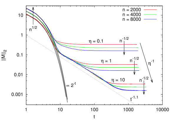
Figure 9: Decrease of the norm of the total magnetization $\|{\bm{M}}({\bm{\sigma}}^{t})\|_{2}$ during block-coordinate ascent. The starting value $\|{\bm{M}}({\bm{\sigma}}^{0})\|_{2}$ is $O(\sqrt{n})$ since the initial configuration is randomly chosen. The asymptotic value is always very small for the sizes studied and decreases as $1/\eta$ and $1/\sqrt{n}$.

In Figure 9 we plot the evolution of the norm of the ‘global magnetization,’ $\|{\bm{M}}({\bm{\sigma}}^{t})\|_{2}$, as a function of the number of iterations $t$. Notice that each iteration corresponds to $n$ updates, one update of each vector ${\bm{\sigma}}_{i}$, $i\in[n]$. We used $d=5$ and $\lambda=1.1$, and we averaged over a number of samples ranging from $100$ (for $n=8000$) to $400$ (for $n=2000$).

We observe three regimes:

• Initially the magnetization decays exponentially, $\|{\bm{M}}({\bm{\sigma}}^{t})\|_{2}\approx\|{\bm{M}}({\bm{\sigma}}^{0})\|_{2}\>2^{-t}$. Further, it increases slowly with $n$. Indeed from central limit theorem, we have $\|{\bm{M}}({\bm{\sigma}}^{0})\|_{2}=\Theta(\sqrt{n})$. The same behavior $\|{\bm{M}}({\bm{\sigma}}^{t})\|_{2}=\Theta(\sqrt{n})$ is found empirically at small $t$.

• In an intermediate interval of times, we have a power law decay $\|{\bm{M}}({\bm{\sigma}}^{t})\|_{2}\propto t^{-a}$, with exponent $a\approx 1.1$. This intermediate regime is present only for $\eta$ large enough.

• For large $t$, $\|{\bm{M}}({\bm{\sigma}}^{t})\|_{2}$ reaches a plateau whose value scales like $\|{\bm{M}}({\bm{\sigma}}^{t})\|_{2}=\Theta(1/\sqrt{n})$ with the system size and is proportional to $1/\eta$.

Already for $\eta=1$, the value of the plateau is very small, namely

$$\left\|\sum_{i=1}^{n}{\bm{\sigma}}_{i}^{t}\right\|_{2}\lesssim 0.1\,.$$ (314)

Further, this value is decreasing with $n$. Given that $\|{\bm{\sigma}}_{i}\|_{2}=1$, we interpret the above as evidence that the constraint $\bm{X}{\mathbf{1}}=0$ is satisfied with good approximation. We will therefore use $\eta=1$ in our simulations.

As an additional remark, notice that there is no special reason to enforce the constraint $\bm{X}{\mathbf{1}}=0$ strictly. Indeed the SDP (191) can be replaced by

maximize $$\;\;\;\;\;\langle\big{(}\bm{A}_{G}-\eta{\mathbf{1}}{\mathbf{1}}^{{\sf T}}\big{)},\bm{X}\rangle\,,$$ (315)

subject to $$\;\;\;\;\;\bm{X}\succeq 0\,,$$ (316)

$$\;\;\;\;\;X_{ii}=1\;\;\forall i\in[n]\,,$$ (317)

with an arbitrary value of $\eta$. Of course this is useful provided $\eta$ is large enough to rule out the solution $\bm{X}={\mathbf{1}}{\mathbf{1}}^{{\sf T}}$. As mentioned above, $\eta\geq d/n$ should be already large enough [MS15].

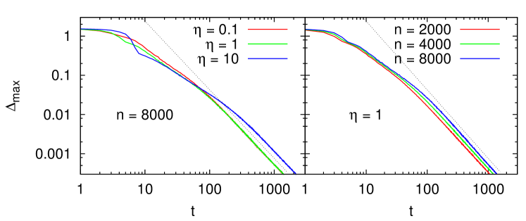
Figure 10: Evolution of ${\mathbb{E}}\Delta_{\text{max}}(t)={\mathbb{E}}\max_{i\in[n]}\|{\bm{\sigma}}_{i}^{t+1}-{\bm{\sigma}}_{i}^{t}\|_{2}$ during block-coordinate ascent. Left panel: dependence on the choice of the Lagrange parameter $\eta$. Right panel: dependence on the number of vertices.

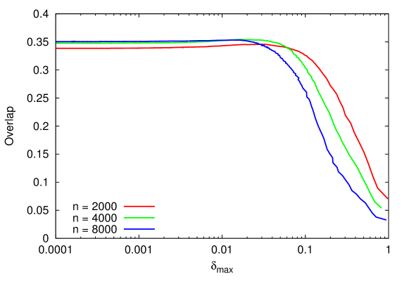
Figure 11: The mean overlap does not depend on the value of ${\mathbb{E}}\Delta_{\text{max}}$ at which the greedy algorithm is stopped, as soon as $\delta_{\text{max}}\lesssim 10^{-3}$.

In Figure 10 we show how $\Delta_{\text{max}}(t)$ decreases with time in Algorithm 4, again with $d=5$ and $\lambda=1.1$.

In the left panel we fix $n=8000$ and study the dependence on the Lagrange parameter $\eta$. We observe two regimes. While for $\eta\lesssim 1$, the convergence rate is roughly independent of $\eta$, for $\eta\gtrsim 1$, it becomes somewhat slower with $\eta$. This supports the choice $\eta=1$.

In the right we fix $\eta=1$ and study the dependence of the convergence time on the graph size $n$. The number of iterations appears to increase slowly with $n$ (see also Figure 12). Both datasets are consistent with a power law convergence

$$\Delta_{\text{max}}(t)\approx C(n)\,t^{-b}\,,$$ (318)

with $b\approx 1.75$ (dotted line), and $C(n)$ polynomially increasing with $n$ (see below for a discussion of the overall scaling of computational complexity with $n$).

In order to select the tolerance parameter for convergence, ${\tt tol}_{3}$, we study the evolution of estimation error. Define the overlap achieved after $t$ iteration as follows. First estimate the vertex labels by computing the top-left singular vector of ${\bm{\sigma}}^{t}$, namely

$$\bm{\hat{x}}^{t}(G)={\rm sign}\big{(}{\bm{v}}_{1}({\bm{\sigma}}^{t}({\bm{\sigma}}^{t})^{{\sf T}})\big{)}\,.$$ (319)

Then define, as before

$${\rm Overlap}_{n}(\bm{\hat{x}}^{t})=\frac{1}{n}{\mathbb{E}}\big{\{}\big{|}\langle\bm{\hat{x}}^{t}(G),\bm{x_{0}}\rangle\big{|}\big{\}}\,.$$ (320)

Of course, the accuracy of the SDP estimator is given by

$${\rm Overlap}_{n}(\bm{\hat{x}}^{\mbox{\tiny{SDP}}})=\lim_{t\to\infty}{\rm Overlap}_{n}(\bm{\hat{x}}^{t})\,.$$ (321)

In Figure 11, we plot ${\rm Overlap}_{n}(\bm{\hat{x}}^{t})$ as a function of ${\mathbb{E}}\Delta_{\max}(t)$ for several values of $n$, $d=5$ and $\lambda=1.1$. These data suggest that ${\tt tol}_{3}=10^{-3}$ is small enough to approximate the $t\to\infty$ behavior. We will fix such a value hereafter.

10.3.2 Selection of $m$ and scaling of convergence times

The last important choice is the value of the dimension (rank) parameter $m$. We know from [MS15] that the optimal value of the rank constrained problem (291) is within a relative error of order $O(1/m)$ of the value of the SDP (288). Also, a result by Burer and Monteiro [BM03] implies that, for $m\geq 2\sqrt{n}$, the objective function (291) has no local maxima that are not also global maxima (barring accidental degeneracies).

We empirically found that $m$ of the order of $10$ or larger is sufficient to obtain accurate results. Through most of our simulations, we fixed however $m=100$, and we want to provide evidence that this is a safe choice

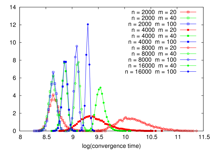
Figure 12: Histograms of the logarithm of the convergence time for the greedy algorithm run with $d=10$ and $\lambda=1$. Red, green and blue histograms are for $m=20,40$ and 100 respectively. System size increases from left to right histograms.

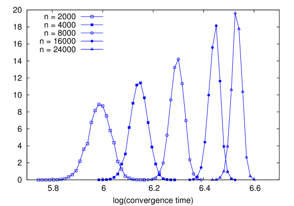
Figure 13: Histograms of the logarithm of the convergence times for $m=100$, $d=10$ and $\lambda=1$.

For each realization of the problem we compute the convergence time $t_{\text{conv}}$ as the first time such that the condition $\Delta_{\max}(t)\leq{\tt tol}_{3}=10^{-3}$ is met. In Figure 12 we plot histograms of $\log(t_{\text{conv}})$ for $n\in\{2000,4000,8000,16000,24000\}$ and $m\in\{20,40,100\}$. Here $d=10$ and $\lambda=1$, but $t_{\text{conv}}$ does not seems to depend strongly on $\lambda$, $d$ in the range we are interested in.

We observe that, for $m$ large enough (in particular $m=100$, see also data in Figure 13), the histogram of $\log(t_{\text{conv}})$ concentrates around its median. We interpret this as evidence of convergence towards a well defined global minimum, whose properties concentrate for $n$ large. On the other hand, for $m$ small, e.g. $m=20$, the histogram broadens as $n$ increases. This is a typical signature of convergence towards local minima, whose properties fluctuate from one graph realization to the other.

Intermediate values of $m$ display a mixed behavior, with the histogram of convergence times concentrating for small $n$ and broadening for larger $n$. This crossover behavior is consistent with the analytical results of [BA06]. Extrapolating this crossover suggests that $m=100$ is sufficient for obtaining very accurate results for the range $n\lesssim 10^{5}$ of interest to us (and most likely, well above).

Focusing on $m=100$ (data in Figure 13), we computed the mean and variance of $\log(t_{\text{conv}})$, for each value of $n$. These appear to be well fitted by the following expressions

$${\mathbb{E}}\log(t_{\text{conv}}) \approx 4.3+0.22\,\log n\,,$$ (322)

$${\rm Var}\Big{(}\log(t_{\text{conv}})\Big{)} \approx 0.063\cdot n^{-1/2}\,.$$ (323)

In other words the typical time complexity of our block coordinate ascent algorithm is –empirically– $O(m\,n^{1.22})$ (recall that each iteration comprises $n$ updates).

10.3.3 Determination of the phase transition location

As already shown in Section 10.2, the overlap ${\rm Overlap}_{n}(\bm{\hat{x}}^{\mbox{\tiny{SDP}}})$ undergoes a phase transition at a critical point $\lambda_{c}^{\mbox{\tiny{SDP}}}(d)$ close to $1$. Namely $\lim_{n\to\infty}{\rm Overlap}_{n}(\bm{\hat{x}}^{\mbox{\tiny{SDP}}})=0$ for $\lambda\leq\lambda_{c}^{\mbox{\tiny{SDP}}}(d)$, while $\lim_{n\to\infty}{\rm Overlap}_{n}(\bm{\hat{x}}^{\mbox{\tiny{SDP}}})>0$ strictly for $\lambda>\lambda_{c}^{\mbox{\tiny{SDP}}}(d)$. In order to determine more precisely the phase transition location, we use the Binder’s cumulant method, which is standard in statistical physics [Bin81, LB14]. We summarize the main ideas of this method for the readers that might not be familiar with this type of analysis.

For a given graph realization $G$, we define $Q(G)$ to be the overlap achieved by the SDP estimator on that realization, i.e.

$$Q(G)\equiv\frac{1}{n}\langle\bm{\hat{x}}^{\mbox{\tiny{SDP}}}(G),\bm{x_{0}}\rangle\,,$$ (324)

Notice that $Q(G)$ is a random variable taking values in $[-1,1]$. Also, by the symmetry of the model, its distribution is symmetric around $0$. Further ${\rm Overlap}_{n}(\bm{\hat{x}}^{\mbox{\tiny{SDP}}})={\mathbb{E}}\{|Q(G)|\}$.

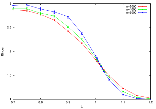
Figure 14: Empirical estimates of the Binder cumulant for $d=5$.

We define the Binder cumulant by

$${\sf Bind}(n,\lambda,d)\equiv\frac{{\mathbb{E}}\big{\{}Q(G)^{4}\big{\}}}{{\mathbb{E}}\big{\{}Q(G)^{2}\big{\}}^{2}}\,.$$ (325)

For $\lambda>\lambda_{c}^{\mbox{\tiny{SDP}}}(d)$, we expect $|Q(G)|$ to concentrate around its expectation ${\rm Overlap}_{n}(\bm{\hat{x}}^{\mbox{\tiny{SDP}}})$, which converges to a non-zero limit. Hence $\lim_{n\to\infty}{\sf Bind}(n,\lambda,d)=1$. On the other hand, for $\lambda>\lambda_{c}^{\mbox{\tiny{SDP}}}(d)$, $Q(G)$ concentrates around $0$, and we expect it to obey a central limit theorem asymptotics, namely $Q(G)\approx{\sf N}(0,\sigma^{2}_{Q}(n))$, with $\sigma^{2}_{Q}(n)\approx\sigma_{Q,*}^{2}/n$. This implies $\lim_{n\to\infty}{\sf Bind}(n,\lambda,d)=3$. Summarizing

$$\lim_{n\to\infty}{\sf Bind}(n,\lambda,d)=\begin{cases}3&\mbox{ if $\lambda<\lambda_{c}^{\mbox{\tiny{SDP}}}(d)$,}\\ 1&\mbox{ if $\lambda>\lambda_{c}^{\mbox{\tiny{SDP}}}(d)$.}\end{cases}$$ (326)

We carried out extensive simulations with the block coordinate ascent, in order to evaluate the Binder cumulant, and will present our data in the next plots. In order to approximate the expectation over the random graph $G$, we computed empirical averages over $N_{\text{sample}}$ random graph samples, with $N_{\text{sample}}$ chosen so that $N_{\text{sample}}\times n=6.4\;10^{8}$. (The rationale for using less samples for larger graph sizes is that we expect statistical uncertainties to decrease with $n$.)

Figure 14 reports a first evaluation of ${\sf Bind}(n,\lambda,d)$ for $d=5$ and a grid of values of $\lambda$. The results are consistent with the prediction of Eq. (326). The approach to the $n\to\infty$ limit is expected to be described by a finite-size scaling ansatz [Car12, LB14]

$${\sf Bind}(n,\lambda,d)\approx{\mathcal{F}}\big{(}n^{1/\nu}(\lambda-\lambda_{c}^{\mbox{\tiny{SDP}}}(d))\big{)}\,,$$ (327)

for a certain scaling function ${\mathcal{F}}$, and exponent $\nu$. Formally, the above approximation is meant to be asymptotically exact in the sense that, for any $z$ fixed, letting $\lambda(z,n)=\lambda_{c}^{\mbox{\tiny{SDP}}}(p)+n^{-1/\nu}z$, we have $\lim_{n\to\infty}{\sf Bind}(n,\lambda(z,n),d)={\mathcal{F}}(z)$. We refer to [BBC⁺01, DM08] for recent examples of rigorous finite-size scaling results in random graph problems.

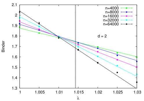
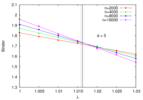
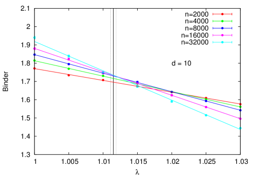
Figure 15: Crossings of the Binder parameters mark the critical value of $\lambda$. Vertical lines are the analytical estimates for the critical point $\tilde{\lambda}_{c}^{\mbox{\tiny{SDP}}}(d)$ (with dashed lines indicating the uncertainty in this estimate, due to numerical solution of the recursive distributional equation).

In particular, finite size scaling suggests to estimate $\lambda_{c}^{\mbox{\tiny{SDP}}}$ by the value of $\lambda$ at which the curves $\lambda\mapsto{\sf Bind}(n,\lambda,d)$, corresponding to different values of $n$, intersect. In Figure 15 we report our data for $d=2$, $5$, $10$, focusing on a small window around the crossing point. Continuous lines are linear fit to the data, and vertical lines correspond to the analytical estimates of Section 9.3.

We observe that, for large $n$, the crossing point is roughly independent of the the value of $n$, in agreement with the finite-size scaling ansatz. As a nominal estimate for the critical point, we use the crossing point $\lambda_{\#}(d)$ of the two Binder cumulant curves corresponding to the two largest values of $n$, see Fig. 15. These are $n=32,000$ and $64,000$ for $d=2$, and $n=16,000$ and $32,000$ for $d=5$, $10$. We obtain

$$\lambda_{\#}(d=2) =1.010\,,$$ (328)

$$\lambda_{\#}(d=5) =1.016\,,$$ (329)

$$\lambda_{\#}(d=10) =1.012\,.$$ (330)

These values are broadly consistent with our analytical prediction for $\tilde{\lambda}_{c}^{\mbox{\tiny{SDP}}}(d)$. There appear to be some discrepancy, especially for $d=2$. This might be due to the graph-size being still too small for extrapolating to $n\to\infty$, or to the inaccuracy of our calculation based on the vectorial ansatz.

10.4 Improving numerical results by restricting to the 2-core

In order to accelerate our numerical experiments presented in Section 10.2 and 10.3, we preprocessed the graph $G$ by reducing it to its $2$-core. Recall that the $k$-core of a graph $G$ is the largest subgraph of $G$, with minimum degree at least $k$. It can be constructed in linear time by recursively removing vertices with degree at most $(k-1)$.

In numerical experiments we first generated $G_{0}$ according to the model (287), then reduced $G_{0}$ to its $2$-core $G$, and finally solved the SDP (288) on $G$. If $G_{0}$ has size $n$, and $d>1$, the size of $G$ is still of order $n$ albeit somewhat smaller [PSW96].

The pruned graph $G\setminus G_{0}$ is formed with high probability by a collection of trees with size of order $1$. It is not hard to see that the SDP estimator can achieve strictly positive overlap on $G_{0}$ (as $n\to\infty$) if and only if it does on $G$. Hence, this reduction does not change the phase transition location. We confirmed numerically this argument as well.

References

- [AB05] D. J. Aldous and A. Bandyopadhyay, A survey of max-type recursive distributional equations, Annals of Applied Probability (2005), 1047–1110.
- [ABBS14] E. Abbe, A. S. Bandeira, A. Bracher, and A. Singer, Decoding binary node labels from censored edge measurements: Phase transition and efficient recovery, Network Science and Engineering, IEEE Transactions on 1 (2014), no. 1, 10–22.
- [ABFM14] Boris Alexeev, Afonso S Bandeira, Matthew Fickus, and Dustin G Mixon, Phase retrieval with polarization, SIAM Journal on Imaging Sciences 7 (2014), no. 1, 35–66.
- [ABH+05] S. Arora, E. Berger, E. Hazan, G. Kindler, and M. Safra, On non-approximability for quadratic programs, Foundations of Computer Science, 2005. FOCS 2005. 46th Annual IEEE Symposium on, IEEE, 2005, pp. 206–215.
- [ALMT14] D. Amelunxen, M. Lotz, M. B. McCoy, and J. A. Tropp, Living on the edge: Phase transitions in convex programs with random data, Information and Inference (2014), iau005.
- [BA06] A. Braun and T. Aspelmeier, The m-component spin glass on a bethe lattice, Physical Review B 74 (2006), no. 14, 144205.
- [BBC+01] B. Bollobás, C. Borgs, J. T. Chayes, J. H. Kim, and D. B. Wilson, The scaling window of the 2-sat transition, Random Structures & Algorithms 18 (2001), no. 3, 201–256.
- [BBS14] A. S. Bandeira, N. Boumal, and A. Singer, Tightness of the maximum likelihood semidefinite relaxation for angular synchronization, arXiv:1411.3272 (2014).
- [BDSY99] A. Ben-Dor, R. Shamir, and Z. Yakhini, Clustering gene expression patterns, Journal of computational biology 6 (1999), no. 3-4, 281–297.
- [Bin81] K. Binder, Finite size scaling analysis of ising model block distribution functions, Zeitschrift für Physik B Condensed Matter 43 (1981), no. 2, 119–140.
- [BLM15] C. Bordenave, M. Lelarge, and L. Massoulié, Non-backtracking spectrum of random graphs: community detection and non-regular ramanujan graphs, Foundations of Computer Science (FOCS), 2015 IEEE 55th Annual Symposium on, 2015.
- [BM03] Samuel Burer and Renato DC Monteiro, A nonlinear programming algorithm for solving semidefinite programs via low-rank factorization, Mathematical Programming 95 (2003), no. 2, 329–357.
- [BSS87] Jayanth R Banavar, David Sherrington, and Nicolas Sourlas, Graph bipartitioning and statistical mechanics, Journal of Physics A: Mathematical and General 20 (1987), no. 1, L1.
- [BW93] E. Brézin and S. R. Wadia, The large n expansion in quantum field theory and statistical physics: from spin systems to 2-dimensional gravity, World scientific, 1993.
- [Car12] J. Cardy, Finite-size scaling, Elsevier, 2012.
- [CDMF09] M. Capitaine, C. Donati-Martin, and D. Féral, The largest eigenvalues of finite rank deformation of large wigner matrices: convergence and nonuniversality of the fluctuations, The Annals of Probability (2009), 1–47.
- [CDS98] S. S. Chen, D. L. Donoho, and M. A. Saunders, Atomic decomposition by basis pursuit, SIAM journal on scientific computing 20 (1998), no. 1, 33–61.
- [CESV15] E. J Candes, Y. C. Eldar, T. Strohmer, and V. Voroninski, Phase retrieval via matrix completion, SIAM Review 57 (2015), no. 2, 225–251.
- [CRT03] A Crisanti, T Rizzo, and T Temesvari, On the parisi-toulouse hypothesis for the spin glass phase in mean-field theory, The European Physical Journal B-Condensed Matter and Complex Systems 33 (2003), no. 2, 203–207.
- [CT07] E. Candés and T. Tao, The Dantzig selector: statistical estimation when p is much larger than n, Annals of Statistics 35 (2007), 2313–2351.
- [CT10] E. J. Candès and T. Tao, The power of convex relaxation: Near-optimal matrix completion, Information Theory, IEEE Transactions on 56 (2010), no. 5, 2053–2080.
- [Cuc15] M. Cucuringu, Synchronization over and community detection in signed multiplex networks with constraints, Journal of Complex Networks (2015), cnu050.
- [DAM15] Y. Deshpande, E. Abbe, and A. Montanari, Asymptotic mutual information for the two-groups stochastic block model, arXiv:1507.08685 (2015).
- [DKMZ11] A. Decelle, F. Krzakala, C. Moore, and L. Zdeborová, Asymptotic analysis of the stochastic block model for modular networks and its algorithmic applications, Physical Review E 84 (2011), no. 6, 066106.
- [DM08] A. Dembo and A. Montanari, Finite size scaling for the core of large random hypergraphs, The Annals of Applied Probability 18 (2008), no. 5, 1993–2040.
- [DM10] , Gibbs measures and phase transitions on sparse random graphs, Brazilian Journal of Probability and Statistics 24 (2010), no. 2, 137–211.
- [DMM09] D. L. Donoho, A. Maleki, and A. Montanari, Message Passing Algorithms for Compressed Sensing, Proceedings of the National Academy of Sciences 106 (2009), 18914–18919.
- [DT05] D. L. Donoho and J. Tanner, Neighborliness of randomly-projected simplices in high dimensions, Proceedings of the National Academy of Sciences 102 (2005), no. 27, 9452–9457.
- [EK10] D. Easley and J. Kleinberg, Networks, crowds, and markets: Reasoning about a highly connected world, Cambridge University Press, 2010.
- [Gau09] C. F. Gauss, Theoria motus corporum coelestium in sectionibus conicis solem ambientium auctore carolo friderico gauss, sumtibus Frid. Perthes et IH Besser, 1809.
- [GN02] M. Girvan and M. Newman, Community structure in social and biological networks, Proceedings of the national academy of sciences 99 (2002), no. 12, 7821–7826.
- [GT02] Francesco Guerra and Fabio Lucio Toninelli, The thermodynamic limit in mean field spin glass models, Communications in Mathematical Physics 230 (2002), no. 1, 71–79.
- [HLL83] P. W. Holland, K. Laskey, and S. Leinhardt, Stochastic blockmodels: First steps, Social Networks 5 (1983), no. 2, 109–137.
- [KBV09] Y. Koren, R. Bell, and C. Volinsky, Matrix factorization techniques for recommender systems, Computer 42 (2009), no. 8, 30–37.
- [Kho06] S. Khot, Ruling out ptas for graph min-bisection, dense k-subgraph, and bipartite clique, SIAM Journal on Computing 36 (2006), no. 4, 1025–1071.
- [KMM+13] F. Krzakala, C. Moore, E. Mossel, J. Neeman, A. Sly, L. Zdeborová, and P. Zhang, Spectral redemption in clustering sparse networks, Proceedings of the National Academy of Sciences 110 (2013), no. 52, 20935–20940.
- [KN12] S. Khot and A. Naor, Grothendieck-type inequalities in combinatorial optimization, Communications on Pure and Applied Mathematics 65 (2012), no. 7, 992–1035.
- [LB14] D. P. Landau and K. Binder, A guide to monte carlo simulations in statistical physics, Cambridge university press, 2014.
- [LKZ15] Thibault Lesieur, Florent Krzakala, and Lenka Zdeborová, Mmse of probabilistic low-rank matrix estimation: Universality with respect to the output channel, arXiv:1507.03857 (2015).
- [LP13] R. Lyons and Y. Peres, Probability on trees and networks, Citeseer, 2013.
- [LPP97] R. Lyons, R. Pemantle, and Y. Peres, Unsolved problems concerning random walks on trees, Classical and modern branching processes, Springer, 1997, pp. 223–237.
- [Lyo90] R. Lyons, Random walks and percolation on trees, The Annals of Probability (1990), 931–958.
- [Mas14] L. Massoulié, Community detection thresholds and the weak ramanujan property, Proceedings of the 46th Annual ACM Symposium on Theory of Computing, ACM, 2014, pp. 694–703.
- [MM09] M. Mézard and A. Montanari, Information, Physics and Computation, Oxford, 2009.
- [MNS12] E. Mossel, J. Neeman, and A. Sly, Stochastic block models and reconstruction, arXiv:1202.1499 (2012).
- [MNS13] , A proof of the block model threshold conjecture, arXiv:1311.4115 (2013).
- [MP01] M. Mézard and G. Parisi, The Bethe lattice spin glass revisited, The European Physical Journal B-Condensed Matter and Complex Systems 20 (2001), no. 2, 217–233.
- [MPV87] M. Mézard, G. Parisi, and M. A. Virasoro, Spin glass theory and beyond, World Scientific, 1987.
- [MPW15] Ankur Moitra, William Perry, and Alexander S Wein, How robust are reconstruction thresholds for community detection?, arXiv:1511.01473 (2015).
- [MRZ14] A. Montanari, D. Reichman, and O. Zeitouni, On the limitation of spectral methods: From the gaussian hidden clique problem to rank one perturbations of gaussian tensors, arXiv:1411.6149 (2014).
- [MS15] A. Montanari and S. Sen, Semidefinite programs on sparse random graphs and their application to community detection, arXiv:1504.05910 (2015).
- [OS08] Reinhold Oppermann and Manuel J Schmidt, Universality class of replica symmetry breaking, scaling behavior, and the low-temperature fixed-point order function of the sherrington-kirkpatrick model, Physical Review E 78 (2008), no. 6, 061124.
- [P+09] A. Plaza et al., Recent advances in techniques for hyperspectral image processing, Remote sensing of environment 113 (2009), S110–S122.
- [PSW96] B. Pittel, J. Spencer, and N. Wormald, Sudden emergence of a giantk-core in a random graph, Journal of Combinatorial Theory, Series B 67 (1996), no. 1, 111–151.
- [Sin11] A. Singer, Angular synchronization by eigenvectors and semidefinite programming, Applied and computational harmonic analysis 30 (2011), no. 1, 20–36.
- [SKZ14] A. Saade, F. Krzakala, and L. Zdeborová, Spectral clustering of graphs with the bethe hessian, Advances in Neural Information Processing Systems, 2014, pp. 406–414.
- [Som83] H-J Sommers, Properties of sompolinsky’s mean field theory of spin glasses, Journal of Physics A: Mathematical and General 16 (1983), no. 2, 447.
- [SS11] A. Singer and Y. Shkolnisky, Three-dimensional structure determination from common lines in cryo-em by eigenvectors and semidefinite programming, SIAM journal on imaging sciences 4 (2011), no. 2, 543–572.
- [SW87] D Sherrington and KYM Wong, Graph bipartitioning and the bethe spin glass, Journal of Physics A: Mathematical and General 20 (1987), no. 12, L785.
- [Tib96] R. Tibshirani, Regression shrinkage and selection with the Lasso, J. Royal. Statist. Soc B 58 (1996), 267–288.
- [Tou80] G Toulouse, On the mean field theory of mixed spin glass-ferromagnetic phases, Journal de Physique Lettres 41 (1980), no. 18, 447–449.
- [VL07] Ulrike Von Luxburg, A tutorial on spectral clustering, Statistics and computing 17 (2007), no. 4, 395–416.
- [Was00] L. Wasserman, Bayesian model selection and model averaging, Journal of mathematical psychology 44 (2000), no. 1, 92–107.
- [WdM15] I. Waldspurger, A. d’Aspremont, and S. Mallat, Phase recovery, maxcut and complex semidefinite programming, Mathematical Programming 149 (2015), no. 1-2, 47–81.