Solving non-linear Horn clauses using a linear solver

Abstract

Developing an efficient non-linear Horn clause solver is a challenging task since the solver has to reason about the tree structures rather than the linear ones as in a linear solver. In this paper we propose an incremental approach to solving a set of non-linear Horn clauses using a linear Horn clause solver. We achieve this by interleaving a program transformation and a linear solver. The program transformation is based on the notion of tree dimension, which we apply to trees corresponding to Horn clause derivations. The dimension of a tree is a measure of its non-linearity – for example a linear tree (whose nodes have at most one child) has dimension zero while a complete binary tree has dimension equal to its height.

A given set of Horn clauses $P$ can be transformed into a new set of clauses $P^{\leq k}$ (whose derivation trees are the subset of $P$’s derivation trees with dimension at most $k$). We start by generating $P^{\leq k}$ with $k=0$, which is linear by definition, then pass it to a linear solver. If $P^{\leq k}$ has a solution $M$, and is a solution to $P$ then $P$ has a solution $M$. If $M$ is not a solution of $P$, we plugged $M$ to $P^{\leq k+1}$ which again becomes linear and pass it to the solver and continue successively for increasing value of $k$ until we find a solution to $P$ or resources are exhausted. Experiment on some Horn clause verification benchmarks indicates that this is a promising approach for solving a set of non-linear Horn clauses using a linear solver. It indicates that many times a solution obtained for some under-approximation $P^{\leq k}$ of $P$ becomes a solution for $P$ for a fairly small value of $k$.

1 Introduction

In this paper we propose an incremental approach to solving a set of non-linear Horn clauses using a linear Horn clause solver. The idea is similar in spirit to the bounded model checking with the following difference. On one hand, the under-approximation we generate is of bounded dimension (see definition 4), which is not finitely nor precisely solvable. On the other hand, each such under-approximation is linear and the solver has to deal with only linear clauses each time. This is achieved by interleaving a program transformation and a linear solver. The program transformation is based on the notion of tree dimension, which we apply to trees corresponding to Horn clause derivations. The dimension of a tree is a measure of its non-linearity – for example a linear tree (whose nodes have at most one child) has dimension zero while a complete binary tree has dimension equal to its height.

We say a set of Horn clause $P$ (including integrity constraints) is solvable iff it has a model. Integrity constraints are special kind of Horn clauses with $\mathsf{false}$ head where $\mathsf{false}$ is always interpreted as $\mathsf{false}$. A given set of Horn clauses $P$ can be transformed into a new set of clauses $P^{\leq k}$ (whose derivation trees are the subset of $P$’s derivation trees with dimension at most $k$). The predicates of $P^{\leq k}$ are subset of predicates of $P$ indexed from $0$ to $k$. We start by generating $P^{\leq k}$ with $k=0$, which is linear by definition, then pass it to a linear solver. If $P^{\leq k}$ has a solution $M$ where $M$ is a set of constrained fact of the form $p_{index}(X)\leftarrow{\cal C}(X)$ for each predicate $p_{index}$ of $P^{\leq k}$. Let $M^{\prime}$ is $M$ after removing index of predicates from each constraint fact in $M$. If $M^{\prime}$ is a solution to $P$ then $P$ has a solution $M^{\prime}$. If $M^{\prime}$ is not a solution of $P$, we plugged $M$ to $P^{\leq k+1}$ which again becomes linear and pass it to the solver and continue successively for increasing value of $k$ until we find a solution to $P$ or resources are exhausted.

Experiment on some Horn clause verification benchmarks indicates that this is a promising approach for solving a set of non-linear Horn clauses. The program transformation allows one to use a linear solver and solution from a previous iteration can be reused in the latter one. Many times a solution obtained for some under-approximation $P^{\leq k}$ becomes inductive, that is, a solution for $P$.

To motivate readers, we present an example set of constrained Horn clauses (CHCs) $P$ in Figure 1 which defines the Fibonacci function. This is an interesting problem whose dimension depends on the input number and its computations are trees rather than linear sequences. The main contributions of this paper are the following.

c1. fib(A, B):- A>=0,  A=<1, B=A. c2. fib(A, B) :- A > 1, A2 = A - 2, fib(A2, B2),            A1 = A - 1, fib(A1, B1), B = B1 + B2. c3. false:- A>5, fib(A,B), B<A.

Figure 1: Example CHCs Fib: it defines a Fibonacci function.

1. We give an iterative algorithm for solving a set of non-linear Horn clauses using a linear solver (Section 3);

2. We demonstrate the feasibility of our approach in practice applying it to non-linear Horn clause verification problems (Section 4);

2 Preliminaries

A constrained Horn clause is a first order formula of the form $p(X)\leftarrow{\cal C},p_{1}(X_{1}),\ldots,p_{k}(X_{k})$ ($k\geq 0$) (using Constraint Logic Programming (CLP) syntax), where ${\cal C}$ is a conjunction of constraints with respect to some background theory, $X_{i},X$ are (possibly empty) vectors of distinct variables, $p_{1},\ldots,p_{k},p$ are predicate symbols, $p(X)$ is the head of the clause and ${\cal C},p_{1}(X_{1}),\ldots,p_{k}(X_{k})$ is the body. A clause is called non-linear if it contains more than one atom in the body ($k>1$), otherwise it is called linear. A set of Horn clauses $P$ is called linear if $P$ only contains linear clauses, otherwise it is called non-linear. A set of Horn clauses is sometimes called a program.

Definition 1 (Solution of Horn clauses)

Let $P$ be a set of Horn claues and $M$ a set of constrained fact of the form $p(X)\leftarrow{\cal C}(X)$, where $p(X)$ is a predicate in $P$ and ${\cal C}(X)$ is an interpretation of $p(X)$ under some constraint theory. Then $M$ is called a solution (model) of $P$ if it satisfies each clause in $P$.

Definition 2 (Inductive solution of Horn clauses)

Let $P_{u}$ be an under-approximation of a set of Horn clauses $P$. If a solution $M$ of $P_{u}$ is also a solution of $P$, then $M$ is called an inductive solution of $P$. In other words, a solution of a particular case (that is an under-approximation) of $P$ becomes a solution of $P$.

A labeled tree $c(t_{1},\ldots,t_{k})$ is a tree with its nodes labeled, where $c$ is a node label and $t_{1},\ldots,t_{k}$ are labeled trees rooted at the children of the node and leaf nodes are denoted by $c$.

Definition 3 (Tree dimension (adapted from [4]))

Given a labeled tree $t=c(t_{1},\ldots,t_{k})$, the tree dimension of $t$ represented as $\mathit{dim}(t)$ is defined as follows:

$$\mathit{dim}(t)=\begin{cases}0&\text{if }k=0\\ \max_{i\in[1..k]}\mathit{dim}(t_{i})&\text{if there is a unique maximum}\\ \max_{i\in[1..k]}\mathit{dim}(t_{i})+1&\text{otherwise }\end{cases}$$

Figure 2 (a) shows a derivation tree $t$ for Fibonacci number 3 and Figure 2 (b) shows its tree dimension. It can be seen that $\mathit{dim}(t)=1$. This number is a measure of its non-linearity, the smaller the number the closer the tree is to a list. Since it is not a perfect binary tree, the height of $t$ (3) is greater than its dimension.

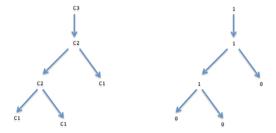
Figure 2: (a) derivation tree of Fibonacci 3 and (b) its tree dimension.

To make the paper self contained, we describe our program transformation approach. Given a set of CHCs $P$ and $k\in\mathbb{N}$, we split each predicate $H$ occurring in $P$ into the predicates $H^{\leq d}$ and $H^{=d}$ where $d\in\{0,1,\ldots,k\}$. Here $H^{\leq d}$ and $H^{=d}$ generate trees of dimension at most $d$ and exactly $d$ respectively.

Definition 4 ( At-most-k-dimension program $P^{\leq k}$)

It consists of the following clauses (adapted from [11, 10]):

1. Linear clauses:

   If $H\leftarrow{\cal C}\in P$ , then $H^{=0}\leftarrow{\cal C}\in P^{\leq k}$.

   If $H\leftarrow{\cal C},B_{1}\in P$ then $H^{=d}\leftarrow{\cal C},B_{1}^{=d}\in P^{\leq k}$ for $0\leq d\leq k$.

2. Non-linear clauses:

   If $H\leftarrow{\cal C},B_{1},B_{2},\ldots,B_{r}\in P$ with $r>1$:

   • For $1\leq d\leq k$, and $1\leq j\leq r$:

     Set $Z_{j}=B_{j}^{=d}$ and $Z_{i}=B_{i}^{\leq d-1}$ for $1\leq i\leq r\wedge i\neq j$. Then: $H^{=d}\leftarrow{\cal C},Z_{1},\ldots,Z_{r}\in P^{\leq k}$.

   • For $1\leq d\leq k$, and $J\subseteq\{1,\ldots,r\}$ with $|J|=2$:

     Set $Z_{i}=B_{i}^{=d-1}$ if $i\in J$ and $Z_{i}=B_{i}^{\leq d-2}$ if $i\in\{1,\ldots,r\}\setminus J$. If all $Z_{i}$ are defined, i.e., $d\geq 2$ if $r>2$, then: $H^{=d}\leftarrow{\cal C},Z_{1},\ldots,Z_{r}\in P^{\leq k}$.

3. $\epsilon$-clauses:

   $H^{\leq d}\leftarrow H^{=e}\in P^{\leq k}$ for $0\leq d\leq k$ , and every $0\leq e\leq d$.

%linear clauses         1. fib(0)(A,A) :- A>=0, A=<1.         2. false(0) :- A>5, B<A, fib(0)(A,B).         %epsilon-clauses         3. false[0] :- false(0).         4. fib[0](A,B) :- fib(0)(A,B).

Figure 3: Fib${}^{\leq 0}:$ at-most-0-dimension program of Fib.

The at-most-0-dimension program of Fib in Figure 1 is depicted in Figure 3. In textual form we represent a predicate $p^{\leq k}$ by p[k] and a predicate $p^{=k}$ by p(k). Since some programs have derivation trees of unbounded dimension, trying to verify a property for its increasing dimension separately is not a practical strategy. It only becomes a viable approach if a solution of $p^{\leq k}$ for some $k\geq 0$ is inductive for $P$ (definition 2).

3 Solving non-linear set of Horn clauses

A procedure for solving a set of non-linear Horn clauses using a linear solver is presented in Algorithm 1. The main procedure SOLVE(P) takes a set of non-linear Horn clause as input and outputs a solution if they are solvable, unknown otherwise. A solution to a set of Horn clause $P$ is an interpretation for the predicates in $P$ that satisfies each clauses in $P$. The procedure makes use of several sub-procedures which will be descirbed next.

KDIM(P,k) produces an at most $k$ dimesional program $P^{\leq k}$ (ref. definition 4). By defintion, $P^{\leq k}$ is linear for $k=0$. For our example program presented in 1, the at-most-0-dimension program is shown in Figure 3 and is linear since there is at most one non-constraint atom in the body of each clauses. SOLVE_LINEAR(P) is an oracle (a linear Horn clause solver) that returns a solution if $P$ is solvable, otherwise unsolvable. The oracle is sound, that is, if SOLVE_LINEAR(P) returns a solution $S$ then $P$ is solvable and $S$ is a solution of $P$, if it returns unsolvable then $P$ is unsolvable. In this paper, we make use of a solver, which is based on abstract interpretation [1] over the domain of convex polyhedra [2]. The solver produces an over-approximation of minimal model of $P$ as a set of constraints facts for each predictes in $P$. In essence, any Horn clause solver can be used. This approximation is regarded as a solution of the claues if there is no constrained fact for $\mathsf{false}$ in it. Using this solver, the following solution is obtained for the program in Figure 3.

fib(0)(A,B) :- [-A>= -1,A>=0,B=1].
fib[0](A,B) :- [-A>= -1,A>=0,B=1].

INDUCTIVE(M, P) checks if a given solution $M$ is a solution of $P$. The predicates of $P^{\leq k}$ are subset of predicates of $P$ indexed from $0$ to $k$. If $P^{\leq k}$ has a solution $M$ where $M$ is a set of constrained fact of the form $p_{index}(X)\leftarrow{\cal C}(X)$ for each predicate $p_{index}$ of $P^{\leq k}$. Let $M^{\prime}$ is $M$ after removing index of predicates from each constraint fact in $M$. If $M^{\prime}$ is a solution to $P$ then $P$ has a solution $M^{\prime}$. If this is the case, then INDUCTIVE(M, P) returns “yes” otherwise “no”. Given the above solution for at-most-0-dimension program, we check if the following ($M^{\prime}$)

fib(A,B) :- [-A>= -1,A>=0,B=1].
fib(A,B) :- [-A>= -1,A>=0,B=1].

is a solution to the program in Figure 1. We can see that it is not the case, since the clause c2 is not satisfied under this solution. It should be noted that after removing the index from $M$ to map the solution to the original program, the resulting solution may be in disjunctive form, which allows a non-disjuntive solver to produce a disjunctive solution. Thanks are due to our program transformation.

The sub-procedure LINEARIZE(P, M) generates a linear set of clauses from $P$ and a set of solution $M$. Given $M$ as a set of constrained facts of the form $p(X)\leftarrow{\cal C}$, the procedure involves in replacing every predicate $p(X)$ in $P$ with ${\cal C}$. This produces a linear set of clauses under the following condition, which is captured by the following lemma 1.

Lemma 1 (Linearisation)

If $S$ is a solution computed for a at-most-k-dimension program ($k\geq 0$) and P is a at-most-(k+1)-dimension program, then the procedure LINEARIZE(P, S) returns a set of linear clauses.

An excerpt from a 1-dimension program of our program in Figure 1 is shown below.

false(1) :- A>5, B<A,  fib(1)(A,B).
fib(1)(A,B) :- A>1, C=A-2, E=A-1, B=F+D,  fib(1)(C,D),  fib[0](E,F).

After plugging in the solution obtained for at-most-0-dimension program, we obtain the following set of clauses (after constraints simplification), which are now linear since the body atom fib[0](E,F) in the second clause is replaced by its solution.

false(1) :-  A>5, B<A, fib(1)(A,B).
fib(1)(A,B) :-  -A>= -2, A>1, A-C=2,  B-D=1, fib(1)(C,D).

Continuing to run our algorithm, the following solution obtained for a 2-dimension program becomes an inductive solution for the program in Figure 1 and the algorithm terminates.

fib(0)(A,B) :- [-A>= -1,A>=0,B=1].
fib[0](A,B) :- [-A>= -1,A>=0,B=1].
fib(1)(A,B) :- [A>=2,A+ -B=0].
fib[1](A,B) :- [A+ -B>= -1,B>=1,-A+B>=0].
fib(2)(A,B) :- [A>=4,-2*A+B>= -3].
fib[2](A,B) :- [A>=0,B>=1,-A+B>=0].

1Procedure SOLVE ($P$)

Input: Set of CHCs $P$

Output: (solved, solution), unknown

2 initialization: $k\leftarrow 0$

3 $P^{\prime}\leftarrow$ KDIM($P,k$) (Definition 4)

4 while true do

5       $(r_{k},S_{k})\leftarrow$ SOLVE_LINEAR($P^{\prime}$)

6       if $r_{k}\neq$ solved then

7            return $unknown$

8       end if

9      $b\leftarrow$ INDUCTIVE($S_{k},P$)

10       if $b=$ yes then

11            return $(solved,S_{k})$

12       end if

13      $P_{k+1}\leftarrow$ KDIM($P,k+1$) (Definition 4)

14       $PL_{k+1}\leftarrow$ LINEARIZE($P_{k+1},S_{k}$)

15      

16      $k\leftarrow k+1$ ; $P^{\prime}\leftarrow PL_{k+1}$

17 end while

18

Algorithm 1 Algorithm for solving a set of Horn clauses

The soundness of the algorithm 1 is captured by the following 1 proposition.

Proposition 1 (Soundness of algorithm 1 )

If Algorithm 1 returns a solution $S$ for a set of clauses $P$ then $P$ is solved and $S$ is in fact a solution of $P$.

4 Experimental results

We implemented our algorithm in the tool called LHornSolver, which is freely available at https://github.com/bishoksan/LHornSolver. Then we carried out an experiment on a set of 9 non-linear CHC verification problems taken from the repository of software verification benchmarks. Our aim in the current paper is not to make a systematic comparison with other verification techniques; these are exploratory experiments whether using a linear solver for non-linear problem solving is practical if at all. The results are summarized in Table 1.

Table 1: Experimental results on non-linear CHC verification problems

Program	Result	Time(ms)	k
addition	safe	4000	1
bfprt	safe	2000	2
binarysearch	safe	2000	1
countZero	safe	2000	1
identity	safe	2000	1
merge	safe	2000	1
palindrome	safe	1000	1
fib	safe	2000	2
revlen	safe	1000	1
avg. time(ms)		2000

In the table Program represents a program, Result- represents a verification result using our approach, Time- is a time to solve the program and k represents a value for which a solution of a at-most-k-dimension program (under-approximation) of a set of clauses $P$ becomes inductive for $P$.

Our current approach solves 9 out of 9 problems with an average time of 2000 milliseconds. These examples were also run on QARMC [6] which solves all the problems ( and much faster).

In most of these problems, a solution of an under approximation (at-most-k-dimension program) becomes a solution for the original one when $k=1$. This shows that a solution for an under-approximation (k-dimension program) becomes inductive for a fairly small value of $k$, and demostrates the feasibility of solving a set of non-linear Horn clauses using a linear solver.

5 Related Work

There exists several Horn clause solvers [7, 5, 12, 8, 9] which handle non-linear clauses. However some tools, for example [3], tackle non-linear clauses by linearising them first and using a linear solver. The generality of the tool such as [3] depends on the class of clauses that are linearisable and it is still not clear which classes of clauses are linearisable and under which conditions. But our approach handles any non-linear clauses and solves them using a linear solver. To the best our knowledge, this is something new.

6 Conclusion and future work

We presented an incremental approach to solving a set of non-linear Horn clauses using a linear Horn clause solver. We presented an algorithm based on this idea which yielded preliminary results on set of non-linear Horn clause verification benchmarks, showing that the approach is feasible.

References

- [1] P. Cousot and R. Cousot. Abstract interpretation: A unified lattice model for static analysis of programs by construction or approximation of fixpoints. In R. M. Graham, M. A. Harrison, and R. Sethi, editors, POPL, pages 238–252. ACM, 1977.
- [2] P. Cousot and N. Halbwachs. Automatic discovery of linear restraints among variables of a program. In Proceedings of the 5th Annual ACM Symposium on Principles of Programming Languages, pages 84–96, 1978.
- [3] E. De Angelis, F. Fioravanti, A. Pettorossi, and M. Proietti. Verimap: A tool for verifying programs through transformations. In E. Ábrahám and K. Havelund, editors, TACAS, volume 8413 of LNCS, pages 568–574. Springer, 2014.
- [4] J. Esparza, S. Kiefer, and M. Luttenberger. On fixed point equations over commutative semirings. In STACS 2007, 24th Annual Symposium on Theoretical Aspects of Computer Science, Proceedings, volume 4393 of LNCS, pages 296–307. Springer, 2007.
- [5] S. Grebenshchikov, A. Gupta, N. P. Lopes, C. Popeea, and A. Rybalchenko. Hsf(c): A software verifier based on Horn clauses - (competition contribution). In C. Flanagan and B. König, editors, TACAS, volume 7214 of LNCS, pages 549–551. Springer, 2012.
- [6] S. Grebenshchikov, N. P. Lopes, C. Popeea, and A. Rybalchenko. Synthesizing software verifiers from proof rules. In J. Vitek, H. Lin, and F. Tip, editors, ACM SIGPLAN Conference on Programming Language Design and Implementation, PLDI ’12, Beijing, China - June 11 - 16, 2012, pages 405–416. ACM, 2012.
- [7] A. Gurfinkel, T. Kahsai, and J. A. Navas. Seahorn: A framework for verifying C programs (competition contribution). In C. Baier and C. Tinelli, editors, Tools and Algorithms for the Construction and Analysis of Systems - 21st International Conference, TACAS 2015, Held as Part of the European Joint Conferences on Theory and Practice of Software, ETAPS 2015, London, UK, April 11-18, 2015. Proceedings, volume 9035 of Lecture Notes in Computer Science, pages 447–450. Springer, 2015.
- [8] K. S. Henriksen, G. Banda, and J. P. Gallagher. Experiments with a convex polyhedral analysis tool for logic programs. In Workshop on Logic Programming Environments, Porto, 2007, 2007.
- [9] B. Kafle and J. P. Gallagher. Tree automata-based refinement with application to horn clause verification. In D. D’Souza, A. Lal, and K. G. Larsen, editors, Verification, Model Checking, and Abstract Interpretation - 16th International Conference, VMCAI 2015, Mumbai, India, January 12-14, 2015. Proceedings, volume 8931 of Lecture Notes in Computer Science, pages 209–226. Springer, 2015.
- [10] B. Kafle, J. P. Gallagher, and P. Ganty. Decomposition by tree dimension in horn clause verification. In press, 2015.
- [11] M. Luttenberger. An extension of parikh’s theorem beyond idempotence. CoRR, abs/1112.2864, 2011.
- [12] P. Rümmer, H. Hojjat, and V. Kuncak. Disjunctive interpolants for Horn-clause verification. In N. Sharygina and H. Veith, editors, CAV, volume 8044 of Lecture Notes in Computer Science, pages 347–363. Springer, 2013.