Study of Sparsity-Aware Distributed Conjugate Gradient Algorithms for Sensor Networks

Abstract

This paper proposes distributed adaptive algorithms based on the conjugate gradient (CG) method and the diffusion strategy for parameter estimation over sensor networks. We present sparsity-aware conventional and modified distributed CG algorithms using $l_{1}$ and log-sum penalty functions. The proposed sparsity-aware diffusion distributed CG algorithms have an improved performance in terms of mean square deviation (MSD) and convergence as compared with the consensus least-mean square (Diffusion-LMS) algorithm, the diffusion CG algorithms and a close performance to the diffusion distributed recursive least squares (Consensus-RLS) algorithm. Numerical results show that the proposed algorithms are reliable and can be applied in several scenarios.

Index Terms—  Distributed Processing, Diffusion Strategy, Conjugate Gradient, Sparsity Aware.

1 Introduction

Distributed processing has become a very common and useful approach to extract information in a network by performing estimation of the desired parameters. The efficiency of the network depends on the communication protocol used to exchange information between the nodes, as well as the algorithm to obtain the parameters. Another important aspect is to prevent a failure in any agent that may affect the operation and the performance of the network. Distributed schemes can offer better estimation performance of the parameters as compared with the centralized approach, based on the principle that each node communicates with several other nodes and exploits the spatial diversity in the networks [1], [36],[37],[38],[39],[40].

The main strategies for communication in distributed processing are incremental, consensus and diffusion. In the incremental protocol, the communication flows cyclically and the information is exchanged from one node to the adjacent nodes. In this strategy the flow of information must be preset at the initialization [2]. The consensus strategy is an elegant procedure to enforce agreement among cooperating nodes [3]. In the diffusion mechanism, each node communicates with the rest of the nodes [4] without any enforcement constraint.

In many scenarios, the parameters of unknown systems can be assumed sparse, containing only a few large coefficients interspersed among many negligible ones [5]. Many studies have shown that exploiting the sparsity of a system is beneficial to enhancing the estimation performance [7]. Most of the studies developed for distributed processing exploiting sparsity [11]-[29] focus on the least-mean square (LMS) and recursive least-squares (RLS) algorithms using different penalty functions [8]-[29]. These penalty functions perform a regularization that attracts to zero the coefficients of the parameter vector that are not associated with the weights of interest. The most well-known and exploited penalty functions are the $l_{0}$-norm, the $l_{1}$-norm and the log-sum [29].

The conjugate gradient (CG) algorithm has been studied and developed for distributed processing [32]-[47]. The faster learning of CG algorithms over the LMS algorithm and its lower computational complexity combined with better numerical stability than the RLS algorithm makes it suitable for this task. However, prior work on distributed CG techniques is rather limited and techniques that exploit possible sparsity of the signals have not been developed so far.

In this paper we propose distributed CG algorithms based on two variants of the diffusion strategy for parameter estimation over sensor networks. Specifically, we develop standard and sparsity-aware distributed CG algorithms using the diffusion protocol and the $l_{1}$ and log-sum penalty functions. The proposed algorithms are compared with recently reported algorithms in the literature. The application scenario in this work is parameter estimation over sensor networks, which can be found in many scenarios of practical interest.

This paper is organized as follows. Section II describes the system model and the problem statement. Section III presents the proposed distributed CG algorithm conventional and modified versions. Section IV details the proposed sparsity-aware distributed diffusion CG algorithm. Section V presents and discusses the simulation results. Finally, Section VI gives the conclusions.

2 System Model and Problem Statement

2.1 System Model

The network consists of N nodes that exchange information between them, where each node represents an adaptive parameter vector with neighborhood described by the set $N_{k}$. The main task of parameter estimation is to adjust the unknown M$\times 1$ weight vector $\boldsymbol{\omega}_{k}$ of each node, where M is the length of the filter [3]. The desired signal $d_{k,i}$ at each time i is drawn from a random process and given by

$$\ d_{k,i}=\boldsymbol{\omega}_{0}^{H}\boldsymbol{x}_{k,i}+n_{k,i}$$ (1)

where $\boldsymbol{\omega}_{0}$ is the M$\times 1$ system weight vector, $\boldsymbol{x}_{k,i}$ is the M$\times 1$ input signal vector and $n_{k,i}$ is the measurement noise. The output estimate is given by

$$\ y_{k,i}=\boldsymbol{\omega}_{k,i}^{H}\boldsymbol{x}_{k,i}$$ (2)

The main goal of the network is to minimize the following cost function:

$$\ C(\boldsymbol{\omega}_{k,i})=\sum_{k=1}^{N}E[|d_{k,i}-\boldsymbol{\omega}_{k,i}^{H}\boldsymbol{x}_{k,i}|^{2}]$$ (3)

By solving this minimization problem it is possible to obtain the optimum solution of the weight vector at each node. The optimum solution for the cost function is given by

$$\ \boldsymbol{\omega}_{k,i}=\boldsymbol{R}_{k,i}^{-1}\boldsymbol{b}_{k,i}$$ (4)

where $\boldsymbol{R}_{k,i}=E[\boldsymbol{x}_{k,i}\boldsymbol{x}_{k,i}^{H}]$ is the M$\times\textit{M}$ correlation matrix of the input data vector $\boldsymbol{x}_{k,i}$, and $\boldsymbol{b}_{k,i}=E[d_{k,i}^{*}\boldsymbol{x}_{k,i}]$ is the M$\times 1$ cross-correlation vector between the input data and $d_{k,i}$.

2.2 Problem Statement

We consider a diffusion algorithm for a network where each agent k has access at each time instant to the realization $\{d_{k,i},\boldsymbol{x}_{k,i}\}$ of zero-mean spatial data $\{d_{k,i},\boldsymbol{x}_{k,i}\}$ [32]-[40]. For a network with possibly sparse parameter vectors, the cost function also involves a penalty function which exploits sparsity. In this case the network needs to solve the following optimization problem:

$$\mbox{min}\ C(\boldsymbol{\omega}_{k,i})=\boldsymbol{\sum}_{k=1}^{N}E[|d_{k,i}-\boldsymbol{\omega}_{k,i}^{H}\boldsymbol{x}_{k,i}|^{2}]+f(\boldsymbol{\omega}_{k,i})$$ (5)

where $f(\boldsymbol{\omega}_{k,i})$ is a penalty function that exploits the sparsity in the parameter vector $\boldsymbol{\omega}_{k,i}$. In the following sections we focus on distributed diffusion CG algorithms to solve (5)

3 Proposed Distributed Diffusion CG Algorithm

In this section, we present the proposed distributed CG algorithm using the diffusion strategy with a penalty function that is equal to zero. This corresponds to the diffusion strategy without the exploitation of sparsity. We first derive the CG algorithm and then consider the diffusion protocol.

3.1 Derivation of the CG algorithm

The CG method can be applied to adaptive filtering problems [30][32][41]. The main objective in this task is to solve (4). The cost function for one agent is given by

$$\ C_{CG}(\boldsymbol{\omega})=\frac{1}{2}\boldsymbol{\omega}^{H}\boldsymbol{R}\omega-\boldsymbol{b}^{H}\boldsymbol{\omega}$$ (6)

For distributed processing over sensor networks, we present the following derivation. The CG algorithm does not need to compute the matrix inversion of $\boldsymbol{R}$, which is an advantage as compared with RLS algorithms. It computes the weights $\boldsymbol{\omega}_{k,i}$ for each iteration j until convergence, i.e., $\boldsymbol{\omega}_{k,i}(j)$. The gradient of the method in the negative direction is obtained as follows [30]:

$$\ \boldsymbol{g}_{k,i}(j)=\boldsymbol{g}_{k,i}(j)-\boldsymbol{R}_{k,i}(j)\boldsymbol{\omega}_{k,i}(j)$$ (7)

Calculating the Krylov subspace [34] through different operations, the recursion is given by

$$\ \boldsymbol{\omega}_{k,i}(j)=\boldsymbol{\omega}_{k,i}(j-1)-\alpha(j)\boldsymbol{p}_{k,i}(j)$$ (8)

where $\boldsymbol{p}$ is the conjugate direction vector of $\boldsymbol{g}$ and $\alpha$ is the step size that minimizes the cost function in (6) by replacing (7) in (4). Both parameters are calculated as follows:

$$\ \alpha(j)=\frac{\boldsymbol{g}_{k,i}^{H}(j-1)\boldsymbol{g}_{k,i}(j-1)}{\boldsymbol{p}_{k,i}^{H}(j)\boldsymbol{R}_{k,i}(j)\boldsymbol{p}_{k,i}(j)}$$ (9)

$$\ \boldsymbol{p}_{k,i}(j)=\boldsymbol{g}_{k,i}(j)+\beta(j)\boldsymbol{p}_{k,i}(j)$$ (10)

The parameter $\beta$ is calculated using the Gram-Schmidt orthogonalization procedure [35] as given by

$$\ \beta(j)=\frac{\boldsymbol{g}_{k,i}^{H}(j)\boldsymbol{g}_{k,i}(j)}{\boldsymbol{g}_{k,i}^{H}(j-1)\boldsymbol{g}_{k,i}(j-1)}$$ (11)

Applying the CG method to a distributed network the cost function is expressed based on the information exchanged between all nodes $k=1,2...,N$. Each of the equations presented so far takes place at each agent during the iterations of the CG algorithm. Therefore, we have the cost function:

$$\ \ \ \ \ \ \ \ \ C_{CG}(\boldsymbol{\omega}_{k,i})=\frac{1}{2}\sum_{k=1}^{N}\boldsymbol{\omega}_{k,i}^{H}\boldsymbol{R}_{k,i}\boldsymbol{\omega}_{k,i}-\boldsymbol{b}_{k,i}^{H}\boldsymbol{\omega}_{k,i}$$ (12)

Using the data window with an exponential decay, the resulting autocorrelation matrix and cross-correlation vector are defined using the forgetting factor $\lambda$ as given by

$$\ \boldsymbol{R}_{k,i}=\lambda\boldsymbol{R}_{k,i-1}+\boldsymbol{x}_{k,i}\boldsymbol{x}_{k,i}^{H}$$ (13)

$$\ \boldsymbol{b}_{k,i}=\lambda\boldsymbol{b}_{k,i-1}+d_{k,i}^{*}\boldsymbol{x}_{k,i}$$ (14)

In the diffusion strategy, all nodes interact with their neighbors sharing and updating the system parameter vector. Each node k is able to run its update simultaneously with the other agents [1] [4]. Figure 1 illustrates the diffusion strategy.

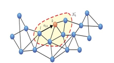
Fig. 1: Distributed consensus-based network processing.

In diffusion protocols there are two well-known variants that switch the order of the combination and adaptation steps, namely, Combine-then-Adapt (CTA) and Adapt-then-Combine (ATC), each one based on the connectivity among nodes. These mechanisms perform adaptation and learning at the same time [3][4].

3.2 CTA Diffusion Distributed CG algorithm

In the CTA diffusion strategy, the convex combination term is first evaluated into an intermediate state variable and subsequently used to perform the weight update [4]. The local estimation is given by

$$\ \boldsymbol{\varphi}_{k,i}=\sum_{l\epsilon N_{k}}a_{lk}\boldsymbol{\omega}_{l,i-1}$$ (15)

where $a_{lk}$ represents the combining coefficients of the data fusion which should comply with

$$\ \sum_{l\epsilon N_{k}}a_{lk}=1,l\epsilon N_{k,i},\forall k.$$ (16)

In this work the strategy adopted for the $a_{lk}$ combiner is the Metropolis rule [1] given by

$$c_{kl}=\left\{\begin{array}[]{ll}\frac{1}{max\{|\mathcal{N}_{k}|,|\mathcal{N}_{l}|\}},\ \ $if\ $k\neq l$\ are linked$\\ 1-\sum\limits_{l\in\mathcal{N}_{k}/k}c_{kl},\ \ $for\ $k$\ =\ $l$$,\end{array}\right.$$ (17)

The distributed CTA CG algorithm based on the derivation steps obtains the updated weight substituting (15) in (8), giving as result:

$$\ \boldsymbol{\omega}_{k,i}(j)=\boldsymbol{\omega}_{k,i}(j-1)-\alpha(j)\boldsymbol{p}_{k,i}(j)$$ (18)

where $\boldsymbol{\omega}_{k,i}(0)=\boldsymbol{\varphi}_{k,i}$ [32]. The rest of the derivation is based on the solution presented in the previous section and the pseudo-code is detailed in Table 1

Table 1: CTA CG ALGORITHM

Parameters initialization:

$\boldsymbol{\omega}_{k,0}=\boldsymbol{0}$

For each time instant $i>0$

For each agent $k$=1,2, …, N

$\boldsymbol{R}_{k,i}=\lambda\boldsymbol{R}_{k,i-1}+\boldsymbol{x}_{k,i}\boldsymbol{x}_{k,i}^{H}$

$\boldsymbol{b}_{k,i}=\lambda\boldsymbol{b}_{k,i-1}+d_{k,i}^{*}\boldsymbol{x}_{k,i}$

$\boldsymbol{\varphi}_{k,i}=\sum_{l\epsilon N_{k}}a_{lk}\omega_{l,i-1}$

$\boldsymbol{\omega}_{k,i}(j)=\boldsymbol{\varphi}_{k,i}$

$\boldsymbol{g}{k,i}(0)=\boldsymbol{b}_{k,i}(0)-\boldsymbol{R}_{k,i}(0)\boldsymbol{\omega}_{k,i-1}$

$\boldsymbol{p}{k,i}(0)=\boldsymbol{g}_{k,i}(0)$

For each CG iteration $j=1$ until convergence

$\alpha(j)=\frac{\boldsymbol{g}_{k,i}^{H}(j-1)\boldsymbol{g}_{k,i}(j-1)}{\boldsymbol{p}_{k,i}^{H}(j)\boldsymbol{R}_{k,i}(j)\boldsymbol{p}_{k,i}(j)}$

$\boldsymbol{\omega}_{k,i}(j)=\boldsymbol{\omega}_{k,i}(j-1)-\alpha(j)\boldsymbol{p}_{k,i}(j)$

$\boldsymbol{g}_{k,i}(j)=\boldsymbol{g}_{k,i}(j)-\alpha(j)\boldsymbol{R}_{k,i}(j)\boldsymbol{p}_{k,i}(j-1)$

$\beta(j)=\frac{\boldsymbol{g}_{k,i}^{H}(j)\boldsymbol{g}_{k,i}(j)}{\boldsymbol{g}_{k,i}^{H}(j-1)\boldsymbol{g}_{k,i}(j-1)}$

$\boldsymbol{p}_{k,i}(j)=\boldsymbol{g}_{k,i}(j)+\beta(j)\boldsymbol{p}_{k,i}(j-1)$

End For

$\boldsymbol{\omega}_{k,i}=\boldsymbol{\omega}_{k,i}(j_{\textit{last}})$

End for

End for

The modified CG (MCG) algorithm comes from the conventional CG algorithm previously presented and only requires one iteration per coefficient update. Specifically, the residual is calculated using (7) (8) and (13) [30]:

$$\begin{array}[]{ll}\ \boldsymbol{g}_{k,i}=\boldsymbol{b}_{k,i}-\boldsymbol{R}_{k,i}\boldsymbol{\varphi}_{k,i}\\[5.69054pt] \ \ \ \ \ \ \ =\lambda\boldsymbol{g}_{k,i-1}-\alpha_{k,i}\boldsymbol{R}_{k,i}\boldsymbol{p}_{k,i-1}\\[5.69054pt] \ \ \ \ \ +\boldsymbol{x}_{k,i}[d_{k,i}-\boldsymbol{\omega}_{k,i-1}^{H}\boldsymbol{x}_{k,i}]\end{array}$$ (19)

The previous equation (19) is multiplied for the search direction vector:

$$\begin{array}[]{ll}\ \boldsymbol{p}_{k,i}^{H}\boldsymbol{g}_{k,i}=\lambda\boldsymbol{p}_{k,i}^{H}\boldsymbol{g}_{k,i-1}-\alpha_{k,i}\boldsymbol{R}_{k,i}\boldsymbol{p}_{k,i-1}\\[5.69054pt] \ \ \ \ \ \ \ \ \ \ \ \ \ \ \ \ \ \ \ \ \ \ +\boldsymbol{p}_{k,i}^{H}\boldsymbol{x}_{k,i}[d_{k,i}-\boldsymbol{\omega}_{k,i-1}^{H}\boldsymbol{x}_{k,i}]\end{array}$$ (20)

Applying the expected value, considering $\boldsymbol{p}_{k,i-1}$ uncorrelated with $\boldsymbol{x}_{k,i}$, $d_{k,i}$ and $\boldsymbol{\varphi}_{k,i}$, and that the algorithm converges the last term of (20) can be neglected. The line search to compute $\alpha$ has to satisfy the convergence bound [11] given by

$$\begin{split}({\lambda_{f}-0.5})\frac{E[\boldsymbol{p}_{k,i-1}^{H}\boldsymbol{g}_{k,i}]}{E[\boldsymbol{p}_{k,i-1}^{H}\boldsymbol{R}_{k,i}\boldsymbol{p}_{k,i-1}]}\leq E[\alpha_{k,i}]\leq\frac{E[\boldsymbol{p}_{k,i-1}^{H}\boldsymbol{g}_{k,i}]}{E[\boldsymbol{p}_{k,i-1}^{H}\boldsymbol{R}_{k,i}\boldsymbol{p}_{k,i-1}]},\end{split}$$ (21)

$$\ \alpha_{k,i}={\eta}\frac{\boldsymbol{p}_{k,i}^{H}\boldsymbol{g}_{k,i}}{\boldsymbol{p}_{k,i}^{H}\boldsymbol{R}_{k,i}\boldsymbol{p}_{k,i}},$$ (22)

where $(\lambda-0.5)\leq\eta\leq\lambda$. The Polak-Ribiere method [30],[31],[33] for the computation of $\beta$ is given by

$$\beta_{k,i}=\frac{(\boldsymbol{g}_{k,i}-\boldsymbol{g}_{k,i-1})^{H}\boldsymbol{g}_{k,i}}{\boldsymbol{g}_{k,i}^{H}\boldsymbol{g}_{k,i}}$$ (23)

3.3 ATC Distributed CG algorithm

Similarly to CTA, the ATC protocol switches the order of the operations. The difference lies in the variable chosen to update the weight $\boldsymbol{\omega}_{k,i}$. In this case, the update estimate is the convex combination of the adaptation step. Table 2 shows the pseudo code of the ATC strategy. The MCG version for the ATC strategy is very similar to the CTA version presented. Table 3 shows the details of the ATC MCG algorithm taking into account the considerations previously discussed.

Table 2: ATC CG ALGORITHM

Parameters initialization:

$\boldsymbol{\omega}_{k,0}=\boldsymbol{0}$

For each time instant $i>0$

For each agent $k$=1,2, …, N

$\boldsymbol{R}_{k,i}=\lambda\boldsymbol{R}_{k,i-1}+\boldsymbol{x}_{k,i}\boldsymbol{x}_{k,i}^{H}$

$\boldsymbol{b}_{k,i}=\lambda\boldsymbol{b}_{k,i-1}+d_{k,i}^{*}\boldsymbol{x}_{k,i}$

$\boldsymbol{g}{k,i}(0)=\boldsymbol{b}_{k,i}(0)-\boldsymbol{R}_{k,i}(0)\boldsymbol{\omega}_{k,i-1}(0)$

$\boldsymbol{p}{k,i}(0)=\boldsymbol{g}_{k,i}(0)$

$\boldsymbol{\omega}_{k,i}(0)=\boldsymbol{\omega}_{k,i-1}$

For each CG iteration $j=1$ until convergence

$\alpha(j)=\frac{\boldsymbol{g}_{k,i}^{H}(j-1)\boldsymbol{g}_{k,i}(j-1)}{\boldsymbol{p}_{k,i}^{H}(j)\boldsymbol{R}_{k,i}(j)\boldsymbol{p}_{k,i}(j)}$

$\boldsymbol{\omega}_{k,i}(j)=\boldsymbol{\omega}_{k,i}(j-1)-\alpha(j)\boldsymbol{p}_{k,i}(j)$

$\boldsymbol{g}_{k,i}(j)=\boldsymbol{g}_{k,i}(j)-\alpha(j)\boldsymbol{R}_{k,i}(j)\boldsymbol{p}_{k,i}(j-1)$

$\beta(j)=\frac{\boldsymbol{g}_{k,i}^{H}(j)\boldsymbol{g}_{k,i}(j)}{\boldsymbol{g}_{k,i}^{H}(j-1)\boldsymbol{g}_{k,i}(j-1)}$

$\boldsymbol{p}_{k,i}(j+1)=\boldsymbol{g}_{k,i}(j)+\beta(j)\boldsymbol{p}_{k,i}(j)$

End For

$\boldsymbol{\omega}_{k,i}=\sum_{l\epsilon N_{k}}a_{lk}\omega_{k,i}(j_{\textit{last}})$

End for

End for

Table 3: ATC MCG ALGORITHM

Parameters initialization:

$\boldsymbol{\omega}_{k,0}=\boldsymbol{0}$

For each time instant $i>0$

For each agent $k$=1,2, …, N

$\boldsymbol{R}_{k,i}=\lambda\boldsymbol{R}_{k,i-1}+\boldsymbol{x}_{k,i}\boldsymbol{x}_{k,i}^{H}$

$\boldsymbol{b}_{k,i}=\lambda\boldsymbol{b}_{k,i-1}+d_{k,i}^{*}\boldsymbol{x}_{k,i}$

$\boldsymbol{\omega}_{k,i}(j)=\boldsymbol{\varphi}_{k,i}$

$\boldsymbol{g}_{k,1}=\boldsymbol{b}_{k,0}$

$\boldsymbol{p}_{k,1}=\boldsymbol{g}_{k,1}$

$\alpha_{k,i}={\eta}\frac{\boldsymbol{p}_{k,i}^{H}\boldsymbol{g}_{k,i}}{\boldsymbol{p}_{k,i}^{H}\boldsymbol{R}_{k,i}\boldsymbol{p}_{k,i}},(\lambda-0.5)\leq\eta\leq\lambda$

$\boldsymbol{\varphi}_{k,i}=\boldsymbol{\omega}_{k,i-1}-\alpha_{k,i}\boldsymbol{p}_{k,i}$

$\boldsymbol{g}_{k,i}=\lambda\boldsymbol{g}_{k,i}-\alpha_{k,i}\boldsymbol{R}_{k,i}\boldsymbol{p}_{k,i-1}$

$+\boldsymbol{x}_{k,i}[d_{k,i}-\boldsymbol{\omega}_{k,i-1}^{H}\boldsymbol{x}_{k,i}]$

$\beta_{k,i}=\frac{(\boldsymbol{g}_{k,i}-\boldsymbol{g}_{k,i-1})^{H}\boldsymbol{g}_{k,i}}{\boldsymbol{g}_{k,i-1}^{H}\boldsymbol{g}_{k,i-1}}$

$\boldsymbol{p}_{k,i}=\boldsymbol{g}_{k,i}+\beta_{k,i}\boldsymbol{p}_{k,i-1}$

End for

$\boldsymbol{\omega}(i)=\sum_{l\epsilon N_{k}}a_{lk}\boldsymbol{\varphi}_{l,i}$

End for

4 Proposed Sparsity-Aware Diffusion CG

Based on the previous development of distributed CG algorithms, this section presents the proposed distributed sparsity-aware diffusion CG algorithms using $l_{1}$ (ZA) and log-sum (RZA) norm penalty functions.

4.1 ZA and RZA CG algorithms

The cost function in this case is given by

$$\ \ \ \ \ \ \ C_{CG}(\boldsymbol{\omega}_{k,i})=\frac{1}{2}\sum_{k=1}^{N}\boldsymbol{\omega}_{k,i}^{H}\boldsymbol{R}\omega_{k,i}-\boldsymbol{b}_{k,i}^{H}\boldsymbol{\omega}_{k,i}+f_{1},$$ (24)

where $f_{1}$ denotes the $l_{1}$ penalty function and is defined by

$$\ f_{1}=\rho\|\boldsymbol{\omega}_{k,i}(j)\|_{1}.$$ (25)

Applying the partial derivative of the penalty function gives

$$\ \ \ \ \ \ \ \frac{\partial(f_{1})}{\partial(\boldsymbol{\omega}_{k,i}^{*})}=sgn(\boldsymbol{\omega}_{k,i})=\left\{\begin{array}[]{ll}\frac{\boldsymbol{\omega}_{k,i}}{|\boldsymbol{\omega}_{k,i}|},\ \ $if\ $\boldsymbol{\omega}_{k,i}\neq 0$$\\ 0,\ \ $if\ $\boldsymbol{\omega}_{k,i}=0$$,\end{array}\right.$$ (26)

When the logarithmic penalty function $f_{2}$ instead $f_{1}$ is used in the cost function, we have

$$\ f_{2}=\rho\sum_{i=1}^{M}\log(1+\frac{|\omega_{k,i}|}{\varepsilon}).$$ (27)

The partial derivative of the penalty function applied with respect to $\boldsymbol{\omega}_{k,i}^{*}$ is described by

$$\ \ \ \ \ \ \ \frac{\partial(f_{1})}{\partial(\boldsymbol{\omega}_{k,i}^{*})}=\frac{sgn(\boldsymbol{\omega}_{k,i})}{1+\varepsilon\|\boldsymbol{\omega}_{k,i}\|_{1}}$$ (28)

In both cases these sparsity-aware algorithms attract to zero the values of the parameter vector which are very small or are not useful. This results in an algorithm with a faster convergence and lower MSD values as can be seen in the following sections. Using the penalty functions (26) and (28), we obtain the sparsity-aware algorithms with the CTA and ATC strategies. Table 4 shows the sparsity-aware method for the ACT protocol. In case of CTA, the same steps applied with the ZA or RZA penalty functions to the steps previously presented in Section III are carried out.

Table 4: Sparsity-aware ATC CG Algorithm

Parameters initialization:

$\boldsymbol{\omega}_{k,0}=\boldsymbol{0}$

For each time instant $i>0$

For each agent $k$=1,2, …, N

$\boldsymbol{R}_{k,i}=\lambda\boldsymbol{R}_{k,i-1}+\boldsymbol{x}_{k,i}\boldsymbol{x}_{k,i}^{H}$

$\boldsymbol{b}_{k,i}=\lambda\boldsymbol{b}_{k,i-1}+d_{k,i}^{*}\boldsymbol{x}_{k,i}$

$\boldsymbol{g}{k,i}(0)=\boldsymbol{b}_{k,i}(0)-\boldsymbol{R}_{k,i}(0)\boldsymbol{\omega}_{k,i-1}(0)$

$\boldsymbol{p}{k,i}(0)=\boldsymbol{g}_{k,i}(0)$

$\boldsymbol{\omega}_{k,i}(0)=\boldsymbol{\omega}_{k,i-1}$

For each CG iteration $j=1$ until convergence

$\alpha(j)=\frac{\boldsymbol{g}_{k,i}^{H}(j-1)\boldsymbol{g}_{k,i}(j-1)}{\boldsymbol{p}_{k,i}^{H}(j)\boldsymbol{R}_{k,i}(j)\boldsymbol{p}_{k,i}(j)}$

$\boldsymbol{\omega}_{k,i}(j)=\boldsymbol{\omega}_{k,i}(j-1)-\alpha(j)\boldsymbol{p}_{k,i}(j)$

$\boldsymbol{g}_{k,i}(j)=\boldsymbol{g}_{k,i}(j)-\alpha(j)\boldsymbol{R}_{k,i}(j)\boldsymbol{p}_{k,i}(j-1)$

$\beta(j)=\frac{\boldsymbol{g}_{k,i}^{H}(j)\boldsymbol{g}_{k,i}(j)}{\boldsymbol{g}_{k,i}^{H}(j-1)\boldsymbol{g}_{k,i}(j-1)}$

$\boldsymbol{p}_{k,i}(j+1)=\boldsymbol{g}_{k,i}(j)+\beta(j)\boldsymbol{p}_{k,i}(j)$

End For

$\boldsymbol{\omega}_{k,i}=\sum_{l\epsilon N_{k}}a_{lk}\omega_{k,i}(j_{\textit{last}})-\rho\frac{\partial(f_{1,2})}{\partial\boldsymbol{\omega}_{k,i}^{*}}$

End for

End for

4.2 ZA and RZA Modified CG algorithms

The ATC and CTA MCG algorithms are very similar as presented in previous section, including the penalty functions. In the ATC strategy, the generation of the first state resulting from the adaptation step, is used in the final update.

4.3 Computational Complexity

The Table 5 shows the computational complexity of all diffusion distributed methods proposed in terms of additions and multiplications.

Table 5: Computational Complexity of diffusion CG algorithms

Method	Additions	Multiplications
CTA-CG	$L(M^{2}+2M)$	$L(2M^{2}+4M)$
	$+LJ(2M^{2}+6M-3)$	$+LJ(3M^{2}+4M-1)$
ATC-CG	$L(M^{2}+3M-1)$	$L(2M^{2}+3M)$
	$+LJ(M^{2}+6M-3)$	$+LJ(3M^{2}+4M-1)$
CTA-MCG	$L(3M^{2}+9M-4)$	$L(4M^{2}+9M-1)$
ATC-MCG	$L(4M^{2}+9M-3)$	$L(6M^{2}+8M-1)$
ZA-CTA-CG	$L(M^{2}+3M)$	$L(2M^{2}+5M)$
	$+LJ(2M^{2}+6M-3)$	$+LJ(3M^{2}+4M-1)$
ZA-ATC-CG	$L(M^{2}+3M)$	$L(2M^{2}+5M)$
	$+LJ(2M^{2}+6M-3)$	$+LJ(3M^{2}+4M-1)$
ZA-CTA-MCG	$L(3M^{2}+10M-4)$	$(4M^{2}+10M-1)$
ZA-ATC-MCG	$L(4M^{2}+10M-3)$	$(6M^{2}+9M-1)$
RZA-CTA-CG	$L(M^{2}+2M)$	$L(2M^{2}+4M)$
	$+LJ(2M^{2}+8M-3)$	$+LJ(3M^{2}+6M-1)$
RZA-ATC-CG	$L(M^{2}+3M-1)$	$L(2M^{2}+3M)$
	$+LJ(2M^{2}+8M-3)$	$+LJ(3M^{2}+6M-1)$
RZA-CTA-MCG	$L(3M^{2}+11M-4)$	$L(4M^{2}+11M-1)$
RZA-ATC-MCG	$L(4M^{2}+11M-3)$	$L(6M^{2}+10M-1)$

It can be seen that the complexity of the modified versions is lower than the conventional methods

5 Simulations Results

In this section, we evaluated the proposed distributed diffusion CG algorithms and compare them with existing algorithms. The results are based on the mean square deviation MSD of the network. We consider a network with $20$ nodes and $1000$ iterations per run. Each iteration corresponds to a time instant. The results are averaged over $100$ experiments. The length of the filter is $10$ and the variance of the input signal 1, which has been modeled as a complex Gaussian noise and the SNR is $30$ dB.

5.1 Comparison between standard and sparsity-aware CTA distributed CG algorithms

For the standard CTA CG version, the system parameter vector was randomly set. In the case of the sparsity-aware algorithms it was set to two values equal to one and the remaining values were set to zero. After all the iterations, the performance of each algorithm in terms of MSD is shown in Fig. LABEL:2. The results show that the sparsity-aware versions outperforms the standard versions and the best results are obtained for the RZA versions. At the same time the MCG algorithms have a better performance than the standard ones.

5.2 Comparison between sparsity-aware ATC distributed CG algorithms.

The same configuration used before was set for CTA strategy. Fig. LABEL:3 below shows the performance of the results in the simulations. Fig. LABEL:4 shows the comparison between the consensus and diffusion algorithms with RZA. It can be observed that the diffusion ATC CG algorithm has a faster convergence as compared to the CTA and consensus strategy, as well as the MSD value at steady state.

6 Conclusions

In this work we proposed distributed CG algorithms for parameter estimation over sensor networks as well as the modified versions of them. The proposed ATC diffusion CG algorithms have a faster convergence than the CTA. The ATC strategy outperforms both consensus[ref] and CTA protocols. In all cases, the modified versions obtained the low MSD values and faster convergence rate. Simulations have shown that the proposed distributed CG algorithms are suitable techniques for adaptive parameter estimation problems.

References

• [1] S. Yuan T, and A. H. Sayed, Diffusion Strategies Outperform Consensus Strategies for Distributed Estimation over Adaptive Networks, IEEE Transactions on signal processing, vol. 60, no. 12, December 2012.
• [2] C. G. Lopes and A. H. Sayed, Incremental adaptive strategies over distributed networks, IEEE Transactions Signal Process, vol. 48, no. 8, pp.223$-$229, Aug 2007.
• [3] M. H. DeGroot, Reaching a consensus, Journal of the American Statistical Association, vol. 69, no. 345, pp. 118-121 ,Mar. 1974.
• [4] A. H. Sayed, Adaptation, Learning, and Optimization over Networks, Foundations and Trends in Machine Learning, vol. 7, no. $4-5$, pp. $311-801$, 2014.
• [5] P. D. Lorenzo and A. H. Sayed, Sparse Distributed Learning Based on Diffusion Adaptation, IEEE Transactions on signal processing, vol. 61, no. 6, March 15, 2013.
• [6] P. Li and R. C. de Lamare, Distributed Iterative Detection With Reduced Message Passing for Networked MIMO Cellular Systems, IEEE Transactions on Vehicular Technology, vol.63, no.6, pp. 2947-2954, July 2014.
• [7] Y. Liu, C. L. and Z. Zhang, Diffusion Sparse Least-Mean Squares Over Networks, IEEE Transactions on Signal Processing, vol. 60, no. 8, August 2012.
• [8] Y. Chen, Y. Gu, and A. O. Hero, Sparse LMS for System Identification, IEEE International Conference on Acoustics, Speech and Signal Processing, ICASSP, April 2009.
• [9] P. D. Lorenzo and S. Barbarossa, Distributed Least Mean Squares Strategies for Sparsity-Aware Estimation over Gaussian Markov Random Fields, IEEE International Conference on Acoustic, Speech and Signal Processing (ICASSP), May 2014.
• [10] E. M. Eksioglu, RLS Adaptive Filtering with Sparsity Regularization, 10th International Conference on Information Science, Signal Processing and their Applications ISSPA, may 2010.
• [11] R. C. de Lamare and R. Sampaio-Neto, β€œAdaptive Reduced-Rank MMSE Filtering with Interpolated FIR Filters and Adaptive Interpolators”, IEEE Signal Processing Letters, vol. 12, no. 3, March, 2005.
• [12] R. C. de Lamare and R. Sampaio-Neto, β€œAdaptive Interference Suppression for DS-CDMA Systems based on Interpolated FIR Filters with Adaptive Interpolators in Multipath Channels”, IEEE Trans. Vehicular Technology, Vol. 56, no. 6, September 2007.
• [13] R. C. de Lamare and R. Sampaio-Neto, β€œReduced-Rank Adaptive Filtering Based on Joint Iterative Optimization of Adaptive Filters, ” IEEE Sig. Proc. Letters, Vol. 14 No. 12, December 2007, pp. 980 - 983.
• [14] M. L. Honig and J. S. Goldstein, β€œAdaptive reduced-rank interference suppression based on the multistage Wiener filter,” IEEE Transactions on Communications, vol. 50, no. 6, June 2002.
• [15] R. C. de Lamare, M. Haardt, and R. Sampaio-Neto, β€œBlind Adaptive Constrained Reduced-Rank Parameter Estimation based on Constant Modulus Design for CDMA Interference Suppression”, IEEE Transactions on Signal Processing, June 2008.
• [16] R. C. de Lamare and R. Sampaio-Neto, β€œSpace time adaptive reduced-rank processor for interference mitigation in DS-CDMA systems”, IET Communications, vol. 2, no. 2, pp. 388-397, 2008.
• [17] R. C. de Lamare and P. S. R. Diniz, ”Set-Membership Adaptive Algorithms based on Time-Varying Error Bounds for CDMA Interference Suppression,” IEEE Trans. Veh. Technol., vol. 58, no. 2, Feb. 2009.
• [18] R. C. de Lamare and R. Sampaio-Neto, β€œAdaptive Reduced-Rank Processing Based on Joint and Iterative Interpolation, Decimation, and Filtering,” IEEE Transactions on Signal Processing, vol. 57, no. 7, July 2009, pp. 2503 - 2514.
• [19] R. C. de Lamare, β€œAdaptive Reduced-Rank LCMV Beamforming Algorithms Based on Joint Iterative Optimisation of Filters,” Electronics Letters, 2008.
• [20] R. C. de Lamare, L. Wang, and R. Fa, β€œAdaptive reduced-rank LCMV beamforming algorithms based on joint iterative optimization of filters: Design and analysis,” Signal Processing, vol. 90, no. 2, pp. 640-652, Feb. 2010.
• [21] R. Fa, R. C. de Lamare, and L. Wang, β€œReduced-Rank STAP Schemes for Airborne Radar Based on Switched Joint Interpolation, Decimation and Filtering Algorithm,” IEEE Transactions on Signal Processing, vol.58, no.8, Aug. 2010, pp.4182-4194.
• [22] R.C. de Lamare, R. Sampaio-Neto, Minimum mean-squared error iterative successive parallel arbitrated decision feedback detectors for DS-CDMA systems , IEEE Trans. Commun., vol. 56, no. 5, May 2008, pp. 778-789.
• [23] R. C. de Lamare, ”Adaptive and Iterative Multi-Branch MMSE Decision Feedback Detection Algorithms for Multi-Antenna Systems”, IEEE Transactions on Wireless Communications, vol. 14, no. 2, February 2013.
• [24] R. C. de Lamare and R. Sampaio-Neto, β€œReduced-Rank Space-Time Adaptive Interference Suppression With Joint Iterative Least Squares Algorithms for Spread-Spectrum Systems,” IEEE Transactions on Vehicular Technology, vol.59, no.3, March 2010, pp.1217-1228.
• [25] R.C. de Lamare, R. Sampaio-Neto and M. Haardt, ”Blind Adaptive Constrained Constant-Modulus Reduced-Rank Interference Suppression Algorithms Based on Interpolation and Switched Decimation,” IEEE Trans. on Signal Processing, vol.59, no.2, pp.681-695, Feb. 2011.
• [26] S. Li, R. C. de Lamare and R. Fa, β€œReduced-Rank Linear Interference Supression for DS-UWB Systems Based on Switched Approximations of Adaptive Basis Functions”, IEEE Transactions on Vehicular Technology, vol. 60, no. 2, February 2011.
• [27] R.C. de Lamare and R. Sampaio-Neto, β€œAdaptive Reduced-Rank Equalization Algorithms Based on Alternating Optimization Design Techniques for MIMO Systems,” IEEE Trans. Vehicular Technology, vol. 60, no. 6, pp.2482-2494, July 2011.
• [28] P. Clarke and R. C. de Lamare, ”Transmit Diversity and Relay Selection Algorithms for Multi-relay Cooperative MIMO Systems”, IEEE Transactions on Vehicular Technology, vol. 61 , no. 3, March 2012, pp. 1084 - 1098.
• [29] R. C. de Lamare and R. Sampaio-Neto, Sparsity-Aware Adaptive Algorithms Based on Alternating Optimization with shrinkage, IEEE Signal Processing Letters, vol. 21, no. 2, February 2014.
• [30] P. S. Chang and A. N. Willson, Jr., Analysis of Conjugate Gradient Algorithms for Adaptive Filtering, IEEE Transactions on Signal Processing, vol. 48, no. 2, February 2000
• [31] L. Wang and R. C. de Lamare, β€œConstrained adaptive filtering algorithms based on conjugate gradient techniques for beamforming,” IET Signal Process., Vol. 4, No. 6, pp. 686–697, Feb 2010.
• [32] S. Xu and R.C de Lamare, , Distributed conjugate gradient strategies for distributed estimation over sensor networks, Sensor Signal Processing for Defense SSPD, September 2012.
• [33] S. Xu, R. C. de Lamare, H. V. Poor, β€œDistributed Estimation Over Sensor Networks Based on Distributed Conjugate Gradient Strategies”, IET Signal Processing, 2016 (to appear).
• [34] O. Axelson, Iterative Solution Methods. New York: Cambridge Univ. Press,1994
• [35] G. H. Golub and C. F. Van Loan, Matrix Computations, 2nd Ed. Baltimore, MD: Johnβ€˜s Hopkins Univ. Press,1989
• [36] S. Xu, R. C. de Lamare and H. V. Poor, Distributed Compressed Estimation Based on Compressive Sensing, IEEE Signal Processing letters, vol. 22, no. 9, September 2014.
• [37] S. Xu, R. C. de Lamare and H. V. Poor, β€œDistributed reduced-rank estimation based on joint iterative optimization in sensor networks,” in Proceedings of the 22nd European Signal Processing Conference (EUSIPCO), pp.2360-2364, 1-5, Sept. 2014
• [38] S. Xu, R. C. de Lamare and H. V. Poor, β€œAdaptive link selection strategies for distributed estimation in diffusion wireless networks,” in Proc. IEEE International Conference onAcoustics, Speech and Signal Processing (ICASSP), , vol., no., pp.5402-5405, 26-31 May 2013.
• [39] S. Xu, R. C. de Lamare and H. V. Poor, β€œDynamic topology adaptation for distributed estimation in smart grids,” in Computational Advances in Multi-Sensor Adaptive Processing (CAMSAP), 2013 IEEE 5th International Workshop on , vol., no., pp.420-423, 15-18 Dec. 2013.
• [40] S. Xu, R. C. de Lamare and H. V. Poor, β€œAdaptive Link Selection Algorithms for Distributed Estimation”, EURASIP Journal on Advances in Signal Processing, 2015.
• [41] S. Wang, H. M. and B. Xi, D. Sun, Conjugate Gradient-based Parameters Identification, 8th IEEE International Conference on Control and Automation, China, June 2010.
• [42] S. Theodoridis, Machine Learning a Bayesian and Optimization Perspective, Academic Press, March 2015.
• [43] I. D. Schizas. G. Mateos and G. B. Giannakis, Distributed LMS for Consensus-Based In-Network Adapting Processing, IEEE Transactions on Signal Processing, vol. 57, no. 6, June 2009
• [44] E. Wei and A. Ozdaglar, Distributed Alternating Direction Method of Multipliers,National Science Foundation under Career grant DMI$-0545910$ and AFOSR MURI FA $9550-09-1-0538$.Department of Electrical Engineering and Computer Science, Massachusetts Institute of Technology.
• [45] X.-L. Feng and T. Z. Huang, A finite-time consensus protocol of the multi-agent systems, World Academy of Science, Engineering and Technology Vol: 5 2011-03-24.
• [46] N. A. Lynch, Distributed algorithms, San Francisco, CA: Morgan Kaufmann, 1997.
• [47] T. G. Miller, S. Xu and R.C de Lamare, , Consensus Distributed Conjugate Gradient Algorithms for Parameter Estimation over Sensor Networks, XXXIII Brazilian Telecommunications Symposium SBrT2015, September 2015.