The local structure of $q$-Gaussian processes

Abstract.

The local structure of $q$-Ornstein–Uhlenbeck process and $q$-Brownian motion are investigated, for all $q\in(-1,1)$. These are classical Markov processes that arose from the study of noncommutative probability. These processes have discontinuous sample paths, and the local small jumps are characterized by tangent processes. It is shown that for all $q\in(-1,1)$, the tangent processes at the interior of the state space are scaled Cauchy processes possibly with drifts. The tangent processes at the boundary of the state space are also computed, but they are not well known processes in classical probability theory. Instead, they can be associated to the free $1/2$-stable law, a well known distribution in free probability, via Biane’s construction.

1. Introduction

In this paper, we investigate the trajectories, particularly the jumps, of certain Markov processes that recently have drawn interest from both classical and noncommutative probability communities. These processes, known as $q$-Gaussian processes, arose from the intriguing connection between noncommutative probability and classical probability described in the seminal work by Bożejko et al., [8]. Since then, the connection has motivated many advances on both Markov processes and their counterparts in noncommutative probability, see for example [7, 12, 9, 1]. Here, we take the classic probability point of view, and we are interested in the local structure of these Markov processes.

In particular, we focus on the so-called $q$-Ornstein–Uhlenbeck process and $q$-Brownian motion for $q\in(-1,1)$. The marginal distribution of the $q$-Ornstein–Uhlenbeck process is a symmetric probability measure supported on closed interval $-2/\sqrt{1-q}\leq x\leq 2/\sqrt{1-q}$ and has probability density function

(1.1) $$p(x)=\frac{\sqrt{1-q}\cdot(q)_{\infty}}{2\pi}\sqrt{4-(1-q)x^{2}}\prod_{k=1}^{\infty}\left[(1+q^{k})^{2}-(1-q)x^{2}q^{k}\right],$$

where $(q)_{\infty}=\prod_{k=1}^{\infty}(1-q^{k})$. This distribution is sometimes called the $q$-normal distribution and appears also as the orthogonality measure of the $q$-Hermite polynomials [15, Section 13.1]. The marginal distribution of the $q$-Brownian motion is just a dilation of (1.1) due to the relation (1.3) below.

It is known that the $q$-normal distribution interpolates between several important distributions as $q$ varies between $-1$ and $1$. When $q=0$ it becomes the celebrated Wigner semicircle law that plays a fundamental role in random matrix theory, when $q$ goes to $1$ it converges to the standard normal distribution that is ubiquitous in classical probability theory, and when $q$ goes to $-1$ it converges to the symmetric discrete distribution on $\{\pm 1\}$ which is sometimes called the Rademacher distribution.

Next, at the process level the transition probabilities of the two Markov processes were identified in [8, Theorem 4.6]. Szabłowski, [19, Section 4] pointed out that they are Feller Markov processes with a càdlàg (right-continuous and left-limit exists) version. Throughout the paper we consider only càdlàg versions of stochastic processes. One can also easily show that as $q$ goes to $1$ the two processes converge in distribution to Brownian motions and Ornstein–Uhlenbeck processes respectively. This roughly says that the paths of $q$-Brownian motion are close to those of the Brownian motion for $q$ close to 1, as illustrated by Figure 1. However, while it is well known that Brownian motions have almost surely continuous paths (e.g. [17]), it has been a folklore that the trajectories of $q$-Brownian motions have jumps, as can also be seen from Figure 1. Our motivation is to understand better these jumps, and hence also the trajectories of $q$-Gaussian processes.

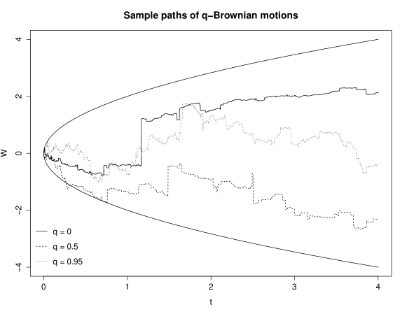
Figure 1. Three trajectories of discretized (in time) $q$-Brownian motions $\{W_{4i/n}^{(q)}\}_{i=0,\dots,n}$ with $q=0,0.5$ and $0.95$ respectively, with $n=2000$, simulated by R. The solid parabolic line ($w^{2}=4t$) is the boundary of the support of the free Brownian motion ($q=0$).

In this paper, we use the notion of tangent process [14] to characterize the local structure of $q$-Gaussian processes, and confirm that while large jumps become unlikely for $q$ close to 1, see Remark 2.7, the two processes are locally approximated by the Cauchy process for every fixed $q<1$, with a possible drift and a multiplicative constant depending on $q$. In order to accomplish our goal, we modify slightly a general framework from Falconer, [14] to allow for dependence on location at time $s\geq 0$. Namely, let $Z=\{Z_{t}\}_{t\geq 0}$ be a càdlàg Markov process, for $s>0$ and $x$ in the support of random variable $Z_{s}$, let $\mathbb{P}(\cdot\mid Z_{s}=x)$ be the law of the Markov process conditioning on $Z_{s}=x$, and we say that $\zeta=\{\zeta_{t}\}_{t\geq 0}$ is a tangent process of $Z$ at time $s$ and location $x$, if under the law $\mathbb{P}(\cdot\mid Z_{s}=x)$ we have weak convergence

(1.2) $$\left\{\frac{Z_{s+\epsilon t}-Z_{s}}{\epsilon^{\beta}}\right\}_{t\geq 0}\Rightarrow\{\zeta_{t}\}_{t\geq 0}$$

as $\epsilon\downarrow 0$, for some $\beta>0$ appropriately chosen, in $D([0,\infty))$ equipped with Skorohod topology. While $Z_{s+\epsilon}$ converges to $Z_{s}$ in probability as $\epsilon\downarrow 0$ for a càdlàg process $Z$, the tangent process in (1.2) provides information on the rates and local fluctuations of the convergence. To establish (1.2), for the two processes it suffices to work with the conditional transition probability densities of $\{Z_{t}\}_{t\geq s}$ given $Z_{s}$, so that the left-hand side induces a unique probability measure on $D([0,\infty))$ [19]. When the tightness is difficult to establish, we consider only convergence of finite-dimensional distributions.

Our main results consist of identifying tangent processes for both $q$-Brownian motions and $q$-Ornstein–Uhlenbeck processes, denoted by $W^{(q)}=\{W_{t}^{(q)}\}_{t\geq 0}$ and $X^{(q)}=\{X_{t}^{(q)}\}_{t\in{\mathbb{R}}}$ respectively throughout the paper. It is well known that for the same $q\in(-1,1)$, these two processes can be mapped onto each other by a deterministic transformation

(1.3) $$\left\{X_{t}^{(q)}\right\}_{t\in{\mathbb{R}}}=\left\{e^{-t}W^{(q)}_{e^{2t}}\right\}_{t\in{\mathbb{R}}}.$$

It is more convenient to work with the $q$-Ornstein–Uhlenbeck process as it is a stationary Markov process on the state space $[-2/\sqrt{1-q},2/\sqrt{1-q}]$. Our findings are summarized as follows.

(i) For $q$-Ornstein–Uhlenbeck process, we first prove that for all $q\in(-1,1)$, the tangent process in (1.2) exists at all location $x\in(-2/\sqrt{1-q},2/\sqrt{1-q})$ with $\beta=1$, and is a Cauchy process up to a multiplicative constant (Theorem 2.1). In other words, locally the $q$-Ornstein–Uhlenbeck process behaves like a Cauchy process, for all $q\in(-1,1)$. It is somehow surprising to see that, although the local jumps disappear in the limit as $q\to 1$, they persist in such a qualitative manner.

(ii) We investigate the tangent process of $q$-Ornstein–Uhlenbeck process at the left boundary point of the state space $x_{-}=-2/\sqrt{1-q}$. In this case, the tangent process still exists as in (1.2), but with scaling parameter $\beta=2$, and is a different Markov process (Proposition 2.2).

(iii) The Markov process obtained as the tangent process at the boundary point seems to have not been well investigated in classical probability theory, to the best of our knowledge. Instead, somehow unexpectedly, we identify this process as the Markov process (up to a quadratic drift) associated to the free $1/2$-stable law via the construction of Biane, [4], after whom we name the process $1/2$-stable Biane process (Proposition 3.1). This connection is irrelevant to the path properties of the processes, but it is of its own interest.

(iv) For the $q$-Brownian motion, since it is not stationary and has inhomogeneous transition probabilities, the situation is slightly more subtle. The tangent process of the $q$-Brownian motion at the interior of the support of $W^{(q)}_{s}$ is still Cauchy, but with a linear drift (Proposition 2.5). The tangent process at time $s$ at the boundary of the support $x_{-}=-2\sqrt{s/(1-q)}$ this time however, instead of in the common form (1.2), appears as the limit of

$$\left\{\frac{W^{(q)}_{s+t\epsilon}+(s(1-q))^{-1/2}\cdot t\epsilon-W^{(q)}_{s}}{\epsilon^{2}}\right\}_{t\geq 0}$$

as $\epsilon\downarrow 0$ under the law $\mathbb{P}(\cdot\mid W_{s}^{(q)}=x_{-})$ (Proposition 2.6). The tangent process turns out to be the $1/2$-stable Biane process up to a multiplicative constant.

The paper is organized as follows. Section 2 establishes limit theorems for the tangent processes at both inner and boundary points for both processes. The connection to noncommutative probability, and particularly the identification of the $1/2$-stable Biane process, are provided in Section 3 in a self-contained manner.

2. Convergence to tangent processes

We first introduce the two processes that appear, with appropriate scalings and drifts, as the tangent processes of $q$-Gaussian processes. Both processes are Markov processes. The first is Cauchy process (symmetric 1-stable Lévy process), starting from $0$ with transition probability density

$$f^{(1)}_{t_{1},t_{2}}(y_{1},y_{2})=\frac{1}{\pi}\frac{t_{2}-t_{1}}{(y_{2}-y_{1})^{2}+(t_{2}-t_{1})^{2}},\;0\leq t_{1}<t_{2}<\infty,y_{1},y_{2}\in{\mathbb{R}}.$$

The second also starts from 0, and has transition probability density

(2.1) $$f^{(1/2)}_{t_{1},t_{2}}(y_{1},y_{2})=\frac{(t_{2}-t_{1})\sqrt{4y_{2}-t_{2}^{2}}}{2\pi\left[(y_{2}-y_{1})^{2}-(t_{2}-t_{1})(t_{1}y_{2}-t_{2}y_{1})\right]},\\ 0\leq t_{1}<t_{2}<\infty,y_{1}>\frac{t_{1}^{2}}{4},y_{2}>\frac{t_{2}^{2}}{4}.$$

Note that the support of the second process at time $t$ is $[t^{2}/4,\infty)$. The two processes are denoted by ${\mathbb{Z}}^{(\alpha)}=\{{\mathbb{Z}}^{(\alpha)}_{t}\}_{t\geq 0}$ with $\alpha=1,1/2$ respectively, and the marginal distributions are given at (3.2) and (3.6) below. Both processes are self-similar with parameter $1/\alpha$ in the sense that

(2.2) $$\left\{{\mathbb{Z}}^{(\alpha)}_{\lambda t}\right\}_{t\geq 0}\stackrel{{\scriptstyle\rm f.d.d.}}{{=}}\lambda^{1/\alpha}\left\{{\mathbb{Z}}^{(\alpha)}_{t}\right\}_{t\geq 0},\lambda>0,\alpha=1,1/2.$$

Furthermore, ${\mathbb{Z}}^{(1)}$ has independent and stationary increments as a Lévy process. The process ${\mathbb{Z}}^{(1/2)}$ has non-stationary increments, but with a drift and time scaling $\{{\mathbb{Z}}^{(1/2)}_{2t}-t^{2}\}_{t\geq 0}$ is self-similar with time-homogeneous transition probability density

(2.3) $$p^{(1/2)}_{t_{1},t_{2}}(y_{1},y_{2})=\frac{2\left(t_{2}-t_{1}\right)\sqrt{y_{2}}}{\pi\left[(y_{2}-y_{1})^{2}+2(y_{1}+y_{2})(t_{2}-t_{1})^{2}+(t_{2}-t_{1})^{4}\right]},y_{1},y_{2},t_{1},t_{2}>0.$$

Both processes also arise from free probability. In particular, ${\mathbb{Z}}^{(1)}$ and ${\mathbb{Z}}^{(1/2)}$ are the Markov processes associated to free $1$-stable and $1/2$-stable semigroups respectively. For the sake of simplicity, we call ${\mathbb{Z}}^{(1/2)}$ the $1/2$-stable Biane process in the sequel. We explain this connection to free probability in the Section 3. The discussion there is independent from the rest of this section, but is of its own interest.

Below, we first consider the tangent processes first $q$-Ornstein–Uhlenbeck processes and then of $q$-Brownian motions.

2.1. Tangent processes of $q$-Ornstein–Uhlenbeck processes

Fix $q\in(-1,1)$, and let $X^{(q)}=\{X^{(q)}_{t}\}_{t\in{\mathbb{R}}}$ denote a $q$-Ornstein–Uhlenbeck process. That is, $X^{(q)}$ is a stationary Markov process with càdlàg trajectories, with the marginal probability density function $p(x)$ given by (1.1), and with the transition probability density function $p_{s,t}(x,y)$ given by, for $x,y\in[-2/\sqrt{1-q},2/\sqrt{1-q}]$,

(2.4) $$p_{s,t}(x,y)=(e^{-2(t-s)};q)_{\infty}\prod_{k=0}^{\infty}\frac{1}{\varphi_{q,k}(t-s,x,y)}\cdot p(y),$$

with

$$\varphi_{q,k}(\delta,x,y)=(1-e^{-2\delta}q^{2k})^{2}-(1-q)e^{-\delta}q^{k}(1+e^{-2\delta}q^{2k})xy+(1-q)e^{-2\delta}q^{2k}(x^{2}+y^{2}).$$

Here and below, we write

$$(a;q)_{\infty}:=\prod_{k=0}^{\infty}(1-aq^{k}),\mbox{ for all }a\in{\mathbb{R}},q\in(-1,1).$$

The above densities can be found at [11, Corollary 2] and [19, Eq.(2.9)].

Two bounds on $\varphi_{q,k}$ are useful. First, observe that $\varphi_{q,k}(\delta,x,y)=a(x^{2}+y^{2})-bx+c$ has a quadratic form with $b/2a>1$. Thus,

$$\min_{|x|,|y|\leq\frac{2}{\sqrt{1-q}}}\varphi_{q,k}(\delta,x,y)=(1-e^{-\delta}q^{k})^{4}\geq(1-|q|^{k})^{4},k\in{\mathbb{N}}_{0},\delta>0.$$

At the same time,

$$\varphi_{q,0}(\delta,x,y) =(1-e^{-2\delta})^{2}-(1-q)e^{-\delta}(1+e^{-2\delta})xy+(1-q)e^{-2\delta}(x^{2}+y^{2})$$

(2.5) $$=e^{-2\delta}\left[4\sinh^{2}(\delta)+(1-q)(x-y)^{2}+2(1-q)xy(1-\cosh(\delta))\right]$$

$$\geq e^{-2\delta}\left[4\sinh^{2}(\delta)+8(1-\cosh(\delta))+(1-q)(x-y)^{2}\right]$$

$$=e^{-2\delta}\left[16\sinh^{4}(\delta/2)+(1-q)(x-y)^{2}\right],$$

where in the inequality above we used the fact that $1-\cosh(\delta)\leq 0$. In particular,

(2.6) $$\prod_{k=0}^{\infty}\frac{1}{\varphi_{q,k}(\delta,x,y)}\leq\frac{e^{2\delta}}{[16\sinh^{4}(\delta/2)+(1-q)(x-y)^{2}](|q|)_{\infty}^{4}}.$$

We first look at the tangent process at the interior of the state space. Consider the process

$$Y^{(\epsilon)}_{t}\mathrel{\mathop{:}}=\frac{X^{(q)}_{\epsilon t}-X^{(q)}_{0}}{\epsilon}.$$

Theorem 2.1.

For all $q\in(-1,1)$, $x\in(-2/\sqrt{1-q},2/\sqrt{1-q})$, under $\mathbb{P}(\cdot\mid X_{0}^{(q)}=x)$, we have

$$\left\{Y^{(\epsilon)}_{t}\right\}_{t\in[0,\infty)}\Rightarrow c_{q,x}\left\{{\mathbb{Z}}^{(1)}_{t}\right\}_{t\in[0,\infty)}\quad\mbox{ with }\quad c_{q,x}=\sqrt{\frac{4}{1-q}-x^{2}}$$

in $D([0,\infty))$ as $\epsilon\downarrow 0$, where ${\mathbb{Z}}^{(1)}$ is the Cauchy process.

Proof.

For $x\in(-2/\sqrt{1-q},2/\sqrt{1-q})$, let $\widetilde{p}_{t_{1},t_{2}}^{(\epsilon,x)}(y_{1},y_{2})$ denote the transition probability density function of $Y^{(\epsilon)}$, conditioning on $X_{0}^{(q)}=x$. Then, writing $\delta:=t_{2}-t_{1}$,

(2.7) $$\widetilde{p}^{(\epsilon,x)}_{t_{1},t_{2}}(y_{1},y_{2})=p_{\epsilon t_{1},\epsilon t_{2}}(x+y_{1}\epsilon,x+y_{2}\epsilon)\epsilon\\ =\frac{\epsilon\sqrt{1-q}\cdot(e^{-2\epsilon\delta};q)_{\infty}(q)_{\infty}}{2\pi}\frac{\sqrt{4-(1-q)(x+y_{2}\epsilon)^{2}}}{\varphi_{q,0}(\epsilon\delta,x+y_{1}\epsilon,x+y_{2}\epsilon)}\prod_{k=1}^{\infty}\frac{\psi_{q,k}(x+y_{1}\epsilon)}{\varphi_{q,k}(\epsilon\delta,x+y_{1}\epsilon,x+y_{2}\epsilon)}$$

with $\psi_{q,k}(x)=(1+q^{k})^{2}-(1-q)x^{2}q^{k}$. We factorize $\widetilde{p}_{t_{1},t_{2}}^{(\epsilon,x)}$ in this way because in the analysis below when computing the limiting probability densities, the infinite product is easy to deal with and contributes asymptotically only a constant, while the square-root term and $\varphi_{q,0}$ contribute to the limiting density and are treated separately. This pattern of calculations will repeatedly show up in all derivations of tangent processes below.

(i) We first prove the convergence of finite-dimensional distributions. For this purpose, by Scheffé’s theorem ([5, Theorem 16.12]) it suffices to prove pointwise convergence of joint probability densities. In particular, we prove

(2.8) $$\lim_{\epsilon\downarrow 0}\widetilde{p}_{t_{1},t_{2}}^{(\epsilon,x)}(y_{1},y_{2})=f^{(1)}_{t_{1},t_{2}}\left(\frac{y_{1}}{c_{q,x}},\frac{y_{2}}{c_{q,x}}\right)\frac{1}{c_{q,x}}.$$

Write $\delta:=t_{2}-t_{1}$. Observe that as $\epsilon\downarrow 0$, recalling (2.5),

$$\varphi_{q,0}(\epsilon\delta,x+y_{1}\epsilon,x+y_{2}\epsilon)\sim\epsilon^{2}\left[(1-q)(y_{2}-y_{1})^{2}+\delta^{2}(4-(1-q)x^{2})\right],$$

and

$$\prod_{k=1}^{\infty} \frac{\psi_{q,k}(x+y_{1}\epsilon)}{\varphi_{q,k}(\epsilon\delta,x+y_{1}\epsilon,x+y_{2}\epsilon)}$$

$$\sim\prod_{k=1}^{\infty}\frac{(1+q^{k})^{2}-(1-q)x^{2}q^{k}}{(1-q^{2k})^{2}-(1-q)q^{k}(1+q^{2k})x^{2}+2(1-q)q^{2k}x^{2}}$$

$$=\prod_{k=1}^{\infty}\frac{(1+q^{k})^{2}-(1-q)x^{2}q^{k}}{(1-q^{k})^{2}(1+q^{k})^{2}-(1-q)x^{2}q^{k}(1-q^{k})^{2}}=\prod_{k=1}^{\infty}\frac{1}{(1-q^{k})^{2}}.$$

Here $y_{1},y_{2}\in{\mathbb{R}}$ are fixed. To pass to the limit, we use the fact that $|q|<1$ and $|x|<2/\sqrt{1-q}$ so the product is bounded by a convergent product uniformly over all small enough $\epsilon$. Small enough means that $\sqrt{1-q}|x+y_{1}\epsilon|<2$ and $\sqrt{1-q}|x+y_{2}\epsilon|<2$.

Finally, we note that

$$(e^{-2\epsilon\delta};q)_{\infty}=(1-e^{-2\epsilon\delta})\prod_{k=1}^{\infty}(1-e^{-2\epsilon\delta}q^{k})\sim 2\epsilon\delta\prod_{k=1}^{\infty}(1-q^{k})=2\epsilon\delta(q)_{\infty}.$$

Combining all the calculation above, we have thus shown

$$\lim_{\epsilon\downarrow 0}p_{\epsilon t_{1},\epsilon t_{2}}(x+y_{1}\epsilon,x+y_{2}\epsilon)\epsilon=\frac{\delta\sqrt{1-q}\sqrt{4-(1-q)x^{2}}}{\pi[(1-q)(y_{2}-y_{1})^{2}+\delta^{2}(4-(1-q)x^{2})]},$$

which is the same as (2.8).

Since our Markov processes start at $0$, the univariate densities also converge, as they are just the transition densities evaluated at $y_{1}=0$ and $t_{1}=0$. We have thus proved the convergence of finite-dimensional distributions.

(ii) Next we prove the tightness. We show that, for all $0\leq t_{1}<t_{2}\leq T<\infty$, $\epsilon>0$, independent of $x$ and $y_{1}$,

(2.9) $${\mathbb{E}}_{x}(|Y_{t_{2}}^{(\epsilon)}-Y_{t_{1}}^{(\epsilon)}|^{2}\wedge 1\mid Y_{t_{1}}^{(\epsilon)}=y_{1})\leq C_{T,q}(t_{2}-t_{1})$$

for some constant $C_{T,q}$ depending only on $T$ and $q$. Then, the tightness of the processes $\{Y^{(\epsilon)}\}_{\epsilon>0}$ under the measure $\mathbb{P}_{x}$ follows from Ethier and Kurtz, [13, Chapter 3, Theorem 8.6, Remark 8.7]. In particular, conditions (8.29) and (8.33) therein are satisfied for our processes.

To prove (2.9), recall (2.6). It then follows that there exists a constant $C_{T,q}$ such that for all $0\leq t_{1}<t_{2}\leq T,\epsilon>0$, uniformly in $x,y_{1},\epsilon$,

$$\widetilde{p}^{x,\epsilon}_{t_{1},t_{2}}(y_{1},y_{2})\leq C_{T,q}\frac{t_{2}-t_{1}}{[(y_{2}-y_{1})^{2}+16\sinh^{4}(\epsilon(t_{2}-t_{1})/2)/(\epsilon^{2}(1-q))]},$$

whence

$${\mathbb{E}}_{x}(|Y_{t_{2}}^{(\epsilon)}-Y_{t_{1}}^{(\epsilon)}|^{2}\wedge 1\mid Y_{t_{1}}^{(\epsilon)}=y_{1})\\ \leq C_{T,q}(t_{2}-t_{1})+\int_{|z|>1}C_{T,q}(t_{2}-t_{1})\frac{1}{z^{2}}dz=C_{T,q}(t_{2}-t_{1}).$$

We have thus proved (2.9) and the tightness. ∎

The proof of Theorem 2.1 does not apply to the boundary points $x=\pm 2/\sqrt{1-q}$. At the same time, as $x\to\pm 2/\sqrt{1-q}$, we have $c_{q,x}\to 0$. These observations raise the question on the tangent process at the boundary, and suggest that for a non-degenerate limit to exist we need to work with a different scaling. Consider the process

$$\widetilde{Y}^{(\epsilon)}_{t}\mathrel{\mathop{:}}=\frac{X_{\epsilon t}-X_{0}}{\epsilon^{2}}.$$

Let $x_{-}=-2/\sqrt{1-q}$ denote the left boundary point.

Proposition 2.2.

For all $q\in(-1,1)$, under $\mathbb{P}(\cdot\mid W_{0}^{(q)}=x_{-})$,

$$\left\{\widetilde{Y}^{(\epsilon)}_{t}\right\}_{t\geq 0}\stackrel{{\scriptstyle\rm f.d.d.}}{{\Longrightarrow}}\frac{4}{\sqrt{1-q}}\left\{{\mathbb{Z}}_{t}^{(1/2)}-\frac{t^{2}}{4}\right\}_{t\geq 0}$$

as $\epsilon\downarrow 0$, where ${\mathbb{Z}}^{(1/2)}$ is the $1/2$-stable Biane process with transition probability densities (2.1).

Remark 2.3.

Here and in Propositions 2.5 and 2.6, we only prove the convergence of finite-dimensional distributions.

Proof.

The proof is similar to the first part of the proof of Theorem 2.1 and consists of verification that the transition density converges. The transition density of $\{\widetilde{Y}^{(\epsilon)}_{t}\}_{t\geq 0}$ is $p_{\epsilon t_{1},\epsilon t_{2}}(x_{-}+y_{1}\epsilon^{2},x_{-}+y_{2}\epsilon^{2})\epsilon^{2}$. With $\delta=t_{2}-t_{1}$, the density factors as in (2.7) with $x$ replaced by $x_{-}$, and we compute the corresponding terms one by one. The infinite product

$$(q)_{\infty}\prod_{k=1}^{\infty}\frac{(1-q^{k}e^{-2\epsilon\delta})\psi_{q,k}(x_{-}+y_{1}\epsilon^{2})}{\varphi_{q,k}(\epsilon\delta,x_{-}+y_{1}\epsilon^{2},x_{-}+y_{2}\epsilon^{2})}$$

converges again to $1$ as $\epsilon\downarrow 0$, and the factor

$$\frac{\epsilon^{2}\sqrt{1-q}\cdot(1-e^{-2\epsilon\delta})}{2\pi}\frac{\sqrt{4-(1-q)(x_{-}+y_{2}\epsilon^{2})^{2}}}{\varphi_{q,0}(\epsilon\delta,x_{-}+y_{1}\epsilon^{2},x_{-}+y_{2}\epsilon^{2})}$$

contributes to the limit. As previously, $(1-e^{-2\epsilon\delta})\sim 2\epsilon\delta$, but at the boundary we have

$$\sqrt{4-(1-q)(x_{-}+y_{2}\epsilon^{2})^{2}}\sim 2\epsilon\sqrt{1-q}\sqrt{y_{2}},$$

and

$$\varphi_{q,0}(\epsilon\delta,x_{-}+y_{1}\epsilon^{2},x_{-}+y_{2}\epsilon^{2})\\ \sim\epsilon^{4}\left[(1-q)(y_{2}-y_{1})^{2}+2\sqrt{1-q}(y_{1}+y_{2})(t_{1}-t_{2})^{2}+(t_{1}-t_{2})^{4}\right].$$

It then follows that

$$\lim_{\epsilon\downarrow 0}p_{\epsilon t_{1},\epsilon t_{2}} (x_{-}+y_{1}\epsilon^{2},x_{-}+y_{2}\epsilon^{2})\epsilon^{2}$$

$$=\frac{2\left(t_{2}-t_{1}\right)\sqrt{(1-q)y_{2}}}{\pi\left[(1-q)(y_{2}-y_{1})^{2}+2\sqrt{1-q}(y_{1}+y_{2})(t_{2}-t_{1})^{2}+(t_{2}-t_{1})^{4}\right]}$$

$$=f_{2t_{1},2t_{2}}^{(1/2)}(\sqrt{1-q}\cdot y_{1}+t_{1}^{2},\sqrt{1-q}\cdot y_{2}+t_{2}^{2})\sqrt{1-q},y_{1},y_{2}>0.$$

The desired result now follows from self-similarity (2.2). ∎

Remark 2.4.

Let $X=\{X_{t}\}_{t\geq 0}$ be a general process. Falconer, [14] actually considers the annealed tangent process, $\{(X_{s+t\epsilon}-X_{s})/\epsilon^{\beta}\}_{t\geq 0}$ for $s\geq 0$, while we consider the quenched tangent process conditioning on the value of $X_{s}$. From our results, the annealed tangent process (without conditioning) can then be derived easily as a mixture of Cauchy process. We omit the details. The same applies to the tangent process of the $q$-Brownian motion in Proposition 2.5.

According to Falconer, [14], for almost all time points $s$ at which the general process $X$ has a unique annealed tangent process, the tangent process must be self-similar with stationary increments. Here we have an example indicating that one cannot drop the ‘almost all’ part of the statement. Indeed, fixing $\tau>0$ and considering $X_{t}=X^{(q)}_{\tau+t}$ with law $\mathbb{P}(\cdot\mid X^{(q)}_{\tau}=x_{-})$, we just showed that for this process at $s=0$, the tangent process exists, is self-similar, but has non-stationary increments. There is no contradiction since as discussed above, for any $s>0$ the annealed tangent process is a mixture of ${\mathbb{Z}}^{(1)}$, and is thus self-similar with stationary increments.

2.2. Tangent processes of $q$-Brownian motions

In this section, consider the $q$-Brownian motion $\{W^{(q)}_{t}\}_{t\geq 0}$ with transition probability density [12, Eq.(55)]

(2.10) $$\kappa_{t_{1},t_{2}}^{(q)}(y_{1},y_{2})=\frac{(1-q)^{3/2}(t_{2}-t_{1})}{2\pi}\frac{\sqrt{4t_{2}-(1-q)y_{2}^{2}}}{\varphi_{q,0}^{*}(t_{1},t_{2},y_{1},y_{2})}\prod_{k=1}^{\infty}\frac{\psi_{q,k}^{*}(t_{1},t_{2},y_{2})}{\varphi_{q,k}^{*}(t_{1},t_{2},y_{1},y_{2})}$$

where

$$\psi_{q,k}^{*}(t_{1},t_{2},y_{2})=(t_{2}-t_{1}q^{k})(1-q^{k+1})\left[t_{2}(1+q^{k})^{2}-(1-q)y_{2}^{2}q^{k}\right],k\geq 1$$

and

$$\varphi_{q,k}^{*}(t_{1},t_{2},y_{1},y_{2})=(t_{2}-t_{1}q^{2k})^{2}-(1-q)q^{k}(t_{2}+t_{1}q^{2k})y_{1}y_{2}+(1-q)(t_{1}y_{2}^{2}+t_{2}y_{1}^{2})q^{2k},k\geq 0.$$

We first consider the tangent process at the interior point of the support of $W^{(q)}_{s}$. For $s>0$, $\epsilon>0$ consider the process

$$\left\{V_{t}^{(\epsilon,s)}\right\}_{t\geq 0}:=\left\{\frac{W^{(q)}_{s+t\epsilon}-W^{(q)}_{s}}{\epsilon}\right\}_{t\geq 0}.$$

Proposition 2.5.

For $s>0$ and $x\in(-2\sqrt{s/(1-q)},2\sqrt{s/(1-q)})$, under the law $\mathbb{P}(\cdot\mid W^{(q)}_{s}=x)$,

$$\left\{V_{t}^{(\epsilon,s)}\right\}_{t\geq 0}\stackrel{{\scriptstyle\rm f.d.d.}}{{\Longrightarrow}}c_{q,s,x}\left\{{\mathbb{Z}}^{(1)}_{t}+\frac{x}{\sqrt{\frac{4s}{1-q}-x^{2}}}\cdot t\right\}_{t\geq 0}$$

as $\epsilon\downarrow 0$, where ${\mathbb{Z}}^{(1)}$ is the Cauchy process and

$$c_{q,s,x}=\frac{1}{2s}\sqrt{\frac{4s}{1-q}-x^{2}}.$$

Proof.

The transition probability density of $V^{(\epsilon,s)}$ conditioning on $W_{s}^{(q)}=x$ is

$$\kappa_{t_{1},t_{2}}^{(\epsilon,s,x)}(y_{1},y_{2}):=\kappa_{s+t_{1}\epsilon,s+t_{2}\epsilon}^{(q)}(x+y_{1}\epsilon,x+y_{2}\epsilon)\epsilon.$$

One can show for all fixed $x\in(-2\sqrt{s/(1-q)},2\sqrt{s/(1-q)})$,

$$\lim_{\epsilon\downarrow 0}\sqrt{4t_{2}-(1-q)y_{2}^{2}}=\sqrt{4s-(1-q)x^{2}},$$

$$\lim_{\epsilon\downarrow 0}\frac{\varphi_{q,0}^{*}(s+t_{1}\epsilon,s+t_{2}\epsilon,x+y_{1}\epsilon,x+y_{2}\epsilon)}{\epsilon^{2}}\\ =(t_{2}-t_{1})^{2}+(1-q)\left[s(y_{2}-y_{1})^{2}-(t_{2}-t_{1})(y_{2}-y_{1})x\right],$$

and

$$\lim_{\epsilon\downarrow 0}\frac{\psi_{q,k}^{*}(s+t_{1}\epsilon,s+t_{2}\epsilon,x+y_{2}\epsilon)}{\varphi_{q,k}^{*}(s+t_{1}\epsilon,s+t_{2}\epsilon,x+y_{1}\epsilon,x+y_{2}\epsilon)}=\frac{1-q^{k+1}}{1-q^{k}},k\geq 1.$$

As previously, the infinite product converges uniformly in $\epsilon$ for all $\epsilon$ close enough to $0$. It then follows that

$$\lim_{\epsilon\downarrow 0}\kappa_{t_{1},t_{2}}^{(\epsilon,s,x)}(y_{1},y_{2})=\frac{1}{2\pi}\frac{\sqrt{1-q}(t_{2}-t_{1})\sqrt{4s-(1-q)x^{2}}}{(t_{2}-t_{1})^{2}+(1-q)[s(y_{2}-y_{1})^{2}-(t_{2}-t_{1})(y_{2}-y_{1})x]}\\ =f^{(1)}_{\tau_{1},\tau_{2}}\left(y_{1}-\frac{t_{1}x}{2s},y_{2}-\frac{t_{2}x}{2s}\right)$$

with $\tau_{j}=\tau_{j}(q,s,x)=c_{q,s,x}t_{j}$ , $j=1,2$. So the limiting process equals in distribution

$$\left\{{\mathbb{Z}}^{(1)}_{c_{q,s,x}t}+\frac{x}{2s}t\right\}_{t\geq 0}\stackrel{{\scriptstyle\rm f.d.d.}}{{=}}c_{q,s,x}\left\{{\mathbb{Z}}^{(1)}_{t}+\frac{x}{\sqrt{\frac{4s}{1-q}-x^{2}}}\cdot t\right\}_{t\geq 0}$$

by self-similarity (2.2). ∎

Next we consider the tangent process at the boundary of the support. Consider the left end-point $x_{-}=-2\sqrt{s/(1-q)}$ of the support of the $q$-Brownian motion at time $s$, and the process

(2.11) $$\widetilde{V}^{(\epsilon,s)}_{t}:=\frac{W^{(q)}_{s+t\epsilon}+at\epsilon-W^{(q)}_{s}}{\epsilon^{2}}\quad\mbox{ with }\quad a=-\frac{2}{(1-q)x_{-}}=\frac{1}{\sqrt{s(1-q)}}.$$

Proposition 2.6.

For all $s>0$, under the law $\mathbb{P}(\cdot\mid W^{(q)}_{s}=x_{-})$,

$$\left\{\widetilde{V}^{(\epsilon,s)}_{t}\right\}_{t\geq 0}\stackrel{{\scriptstyle\rm f.d.d.}}{{\Longrightarrow}}\frac{1}{s^{3/2}\sqrt{1-q}}\left\{{\mathbb{Z}}_{t}^{(1/2)}\right\}_{t\geq 0}$$

as $\epsilon\downarrow 0$, where ${\mathbb{Z}}^{(1/2)}$ is the $1/2$-stable Biane process with transition probability densities (2.1).

Proof.

The transition probability density of $\widetilde{V}_{t}(\epsilon,s)$ under the law $\mathbb{P}(\cdot\mid W^{(q)}_{s}=x_{-})$ is

$$\overline{\kappa}^{(\epsilon,s)}_{t_{1},t_{2}}(y_{1},y_{2})=\kappa^{(q)}_{s+t_{1}\epsilon,s+t_{2}\epsilon}(x_{-}-at_{1}\epsilon+y_{1}\epsilon^{2},x_{-}-at_{2}\epsilon+y_{2}\epsilon^{2})\epsilon^{2}.$$

Again from (2.10), by straight-forward calculation one obtains as $\epsilon\downarrow 0$,

$$\sqrt{4(s+t_{2}\epsilon)-(1-q)(x_{-}-at_{2}\epsilon+y_{2}\epsilon)^{2}}\sim\epsilon\sqrt{4\sqrt{s(1-q)}y_{2}-\frac{t_{2}^{2}}{s}},$$

$$\varphi_{q,0}^{*}(s+t_{1}\epsilon,s+t_{2}\epsilon,x_{-}-at_{1}\epsilon+y_{1}\epsilon^{2},x_{-}-at_{2}\epsilon+y_{2}\epsilon^{2})\\ \sim\epsilon^{4}\left[s(1-q)(y_{2}-y_{1})^{2}-\sqrt{\frac{1-q}{s}}(t_{2}-t_{1})(t_{1}y_{2}-t_{2}y_{1})\right],$$

and

$$\lim_{\epsilon\downarrow 0}\frac{\psi_{q,k}^{*}(s+t_{1}\epsilon,s+t_{2}\epsilon,x-a\epsilon+y_{2}\epsilon^{2})}{\varphi_{q,k}^{*}(s+t_{1}\epsilon,s+t_{2}\epsilon,x-a\epsilon+y_{1}\epsilon^{2},x-a\epsilon+y_{2}\epsilon^{2})}=\frac{1-q^{k+1}}{1-q^{k}},k\geq 1.$$

Again, the infinite product of $\psi^{*}_{q,k}/\varphi^{*}_{q,k}$ converges uniformly for $\epsilon$ small enough as before. We thus arrive at

$$\lim_{\epsilon\downarrow 0}\overline{\kappa}^{(\epsilon,s)}_{t_{1},t_{2}}(y_{1},y_{2})=\frac{\sqrt{1-q}}{2\pi}\frac{(t_{2}-t_{1})\sqrt{4\sqrt{s(1-q)}y_{2}-{t_{2}^{2}}/s}}{s(1-q)(y_{2}-y_{1})^{2}-\frac{\sqrt{1-q}}{\sqrt{s}}(t_{2}-t_{1})(t_{1}y_{2}-t_{2}y_{1})}\\ =f^{(1/2)}_{{t_{1}},{t_{2}}}\left(\sqrt{s^{3}(1-q)}y_{1},\sqrt{s^{3}(1-q)}y_{2}\right)\sqrt{s^{3}(1-q)}.$$

The desired result now follows. ∎

Remark 2.7.

The tangent processes are established for fixed $q$, and they do not capture the behavior of large jumps as $q$ varies. To see what happens as $q$ approaches $1$, we only mention here an explicit estimate

(2.12) $$\mathbb{P}\left(\sup_{S\leq t\leq T}|W^{(q)}_{t-}-W^{(q)}_{t}|>a\right)\leq\frac{(1-q)}{a^{4}}(T^{2}-S^{2}),\quad 0\leq S<T,a>0,$$

which indicates that large jumps become unlikely when $q$ is close to $1$ or when the time interval $T-S$ is small. However, the inequality only provides an upper bound. A precise estimate of the asymptotic probability of large jumps will be established in the form of a Poisson limit theorem in another paper.

To prove (2.12) we use the formula

$${\mathbb{E}}(W^{(q)}_{t}-W^{(q)}_{s})^{4}=(2+q)(t-s)^{2}+2(1-q)s(t-s),\quad 0\leq s<t.$$

which can be read out from [19, formula (4.14)]. With $t_{i}=S+i(T-S)/n$, we have

(2.13) $$\mathbb{P}\left(\max_{i=1,\dots,n}|W^{(q)}_{t_{i}}-W^{(q)}_{t_{i-1}}|>a\right)\leq\frac{1}{a^{4}}\sum_{i=1}^{n}{\mathbb{E}}(W^{(q)}_{t_{i}}-W^{(q)}_{t_{i-1}})^{4}\\ =\frac{2+q}{a^{4}}\sum_{i=1}^{n}(t_{i}-t_{i-1})^{2}+\frac{2(1-q)}{a^{4}}\sum_{i=1}^{n}t_{i-1}(t_{i}-t_{i-1})\to\frac{2(1-q)}{a^{4}}\int_{S}^{T}t\,dt\mbox{ as $n\to\infty$}.$$

For every trajectory, $\max_{i=1,\dots,n}|W^{(q)}_{t_{i}}-W^{(q)}_{t_{i-1}}|$ converges to $\sup_{S<t\leq T}|W^{(q)}_{t-}-W^{(q)}_{t}|$, because for every $\varepsilon>0$ and every a càdlàg function there exist a finite partition of $[0,T]$ into intervals on which the modulus of continuity is less than $\varepsilon$ (see e.g. [6]). Since process $(W^{(q)}_{t})$ is continuous in probability,

$$\sup_{S<t\leq T}|W^{(q)}_{t-}-W^{(q)}_{t}|=\sup_{S\leq t\leq T}|W^{(q)}_{t-}-W^{(q)}_{t}|$$

with probability one. Thus (2.12) follows from (2.13).

3. Connection to free probability

In this section, we explain how the tangent processes ${\mathbb{Z}}^{(1/2)},{\mathbb{Z}}^{(1)}$ are connected to free probability. For this purpose, we first recall the notion of free convolution and free-convolution semigroup in free probability. Free convolution of measures is a free-probability analog of the convolution of measures. While convolution describes the law of the sum of independent random variables, free convolution describes that law of the sum of free noncommutative random variables. Both operations can also be introduced analytically: convolution corresponds to multiplication of the characteristic functions, and free convolution corresponds to addition of the so called the $R$-transforms.

To recall the analytic definition of free convolution, denote by

$$G_{\nu}(z)=\int\frac{\nu(dx)}{z-x}$$

the Cauchy-Stieltjes transform of a probability measure $\nu$ on the Borel sets of the real line. It is known that $G_{\mu}$ is a well defined analytic function in the complex upper plane $z\in\mathbb{C}^{+}=\{z=x+iy:y>0\}$ with the right inverse $K_{\nu}(z)=G^{-1}_{\nu}(z)$ which is well defined for $z$ in a Stolz cone of the form $\{z=x+iy:|x|<\alpha y,|z|\leq\beta\}$. The $R$-transform of the probability measure $\nu$ is then defined as

(3.1) $$R_{\nu}(z)=K_{\nu}(z)-1/z$$

and the free convolution of two measures $\mu$ and $\nu$ is a (unique) probability measure, denoted by $\mu\boxplus\nu$ with the $R$-transform $R_{\mu}(z)+R_{\nu}(z)$ on the common domain. These results, at increasing levels of generality, have been established by Voiculescu, [20], Maassen, [16], and Bercovici and Voiculescu, [3].

A free-convolution semigroup $\{\nu_{t}\}_{t\geq 0}$ is the family of measures such that $\nu_{t+s}=\nu_{t}\boxplus\nu_{s}$, with $\nu_{0}=\delta_{0}$ is a degenerate measure. For example, the family of Cauchy measures

(3.2) $$\nu_{t}^{(1)}(dx)=\frac{t}{\pi(x^{2}+t^{2})}dx,t>0,$$

with Cauchy-Stieltjes transforms $G_{\nu_{t}^{(1)}}(z)=1/(z+it)$ and $R_{\nu_{t}^{(1)}}(z)=it$ on $\mathbb{C}^{+}$, is a free-convolution semigroup, see [3, Section 7] or [4, Example 5.1].

In the seminal paper [4], Biane associated to every free-convolution semigroup $\{\nu_{t}\}_{t\geq 0}$ a classical Markov process $\{{\mathbb{Z}}_{t}\}_{t\geq 0}$ such that the marginal distribution at time $t$ is $\nu_{t}$, and the transition probabilities $Q_{s,t}(x,dy)$ are determined as follows. Fix $s<t$ and $x\in{\mathbb{R}}$. Let $F$ be an analytic function on $\mathbb{C}\setminus\mathbb{R}$ such that

(3.3) $$\int\frac{\nu_{t}(dx)}{z-x}=\int\frac{\nu_{s}(dx)}{F(z)-x}\mbox{ for $z\in\mathbb{C}^{+}$ }.$$

(Note that $F$ depends on $s<t$, but not $x$.) Biane, [4] proved that such mapping exists and is uniquely determined by the requirements that

(3.4) $$\mbox{$F(\bar{z})=\overline{F(z)}$, $F(\mathbb{C}^{+})\subset\mathbb{C}^{+}$, $\Im F(z)\geq\Im z$ and $\lim_{y\to\infty}\frac{F(iy)}{iy}=1$}.$$

Furthermore, Biane showed that $\mathbb{C}^{+}\ni z\mapsto 1/(F(z)-x)\in\mathbb{C}^{-}$ is a Cauchy–Stieltjes transform, so it defines a unique probability measure $Q_{s,t}(x,dy)$ such that

(3.5) $$\int\frac{1}{z-y}Q_{s,t}(x,dy)=\frac{1}{F(z)-x}.$$

The probability measures $\{Q_{s,t}(x,dy):s\leq t,x\in\mathbb{R}\}$ satisfy Chapman–Kolmogorov equations, are Feller (i.e. the map $x\mapsto Q_{s,t}(x,dy)$ is weakly continuous) and $Q_{0,t}(0,dy)=\nu_{t}(dy)$; hence they are transition probabilities of a Markov process, denoted by $\{{\mathbb{Z}}_{t}\}_{t\geq 0}$. We refer to the so-determined Markov process $\{{\mathbb{Z}}_{t}\}_{t\geq 0}$ as the Biane process associated to the free-convolution semigroup $\{\nu_{t}\}_{t\geq 0}$.

Now recall the processes ${\mathbb{Z}}^{(1)}$ and ${\mathbb{Z}}^{(1/2)}$ described in Section 2. First, for the Cauchy process ${\mathbb{Z}}^{(1)}$, it is well known that Cauchy distribution generates also the free $1$-stable semigroup and by [4, Section 5.1] the Cauchy process is indeed the Markov process associated to the free $1$-stable semigroup (3.2). So the Cauchy process is the 1-stable Biane process. Second, the free 1/2-stable semigroup density appears in Bercovici and Pata, [2, page 1054], see also [18, Example 3.2]. The corresponding free-convolution semigroup of measures is then easily determined from rescaling, which gives

(3.6) $$\nu_{t}^{(1/2)}(dx)=\frac{t\sqrt{4x-t^{2}}}{2\pi x^{2}}1_{(t^{2}/4,\infty)}dx,t>0.$$

We show that ${\mathbb{Z}}^{(1/2)}$ defined by (2.1) is the Biane process associated to $\{\nu^{(1/2)}_{t}\}_{t\geq 0}$.

Proposition 3.1.

The Biane process associated to (3.6) is ${\mathbb{Z}}^{(1/2)}$.

Proof.

To determine transition probabilities of the Markov process ${\mathbb{Z}}_{t}$, we start from the Cauchy–Stieltjes transform

(3.7) $$G_{t}(z):=\int\frac{\nu^{(1/2)}_{t}(dx)}{z-x}=\frac{t\sqrt{t^{2}-4z}-t^{2}+2z}{2z^{2}}$$

of the free $1/2$-stable law (3.6). The Cauchy–Stieltjes transform of the closely related measure $\mu_{t}(A)=\nu^{(1/2)}_{t}(-A),A\in{\mathcal{B}}({\mathbb{R}})$ appears explicitly in [10, page 590]. We will present a straightforward calculation of (3.7) using basic complex analysis at the end of this section.

Next, we use the standard branch of the square root, and (3.7) simplifies to

(3.8) $$G_{t}(z)=-\frac{4}{\left(\sqrt{t^{2}-4z}+t\right)^{2}}.$$

The latter is the most convenient form for the equation (3.3) which says that $G_{t}(z)=G_{s}(F(z))$. Using (3.8), we first solve $(\sqrt{t^{2}-4z}+t)^{2}=(\sqrt{s^{2}-4F(z)}+s)^{2}$ for real $z<t/2$ fixed, seeking the real negative solution $F(z)<s/2$. The equation becomes

$$t-s+\sqrt{t^{2}-4z}=\sqrt{s^{2}-4F(z)}.$$

Since $s<t$, both sides are positive, so we get

(3.9) $$F(z)=\frac{1}{4}\left[s^{2}-\left(t-s+\sqrt{t^{2}-4z}\right)^{2}\right].$$

Formula (3.9) has a unique analytic extension to all complex $z$ from the slit plane $\mathbb{C}\setminus[t^{2}/4,\infty)$; the extension amounts to choosing the standard branch of the square root. One can check that with this choice of the root, $F(z)$ given by (3.9) satisfies the uniqueness conditions (3.4). Therefore, (3.5) determines the transition probabilities of the Markov process $({\mathbb{Z}}_{t})$ and specifies their Cauchy–Stieltjes transform as

$$\frac{4}{s^{2}-4x-(t-s+\sqrt{t^{2}-4z})^{2}}.$$

The calculations turn out to be easier if we work with the process $\{{\mathbb{Z}}^{(1/2)}_{2t}-t^{2}\}_{t\geq 0}$ by recasting (3.5) via changing the variables in the above Cauchy–Stieltjes transform, first by replacing $s,t$ by $2s,2t$ and then replacing $x$ by $s^{2}+x$ and $z$ by $z+t^{2}$. This results in a somewhat simpler identity

(3.10) $$\int_{0}^{\infty}\frac{1}{z-y}p^{(1/2)}_{s,t}(x,y)dy=\frac{1}{-x-(t-s+\sqrt{-z})^{2}}=:H_{s,t,x}(z)$$

that we need to prove, with $p^{(1/2)}_{s,t}(x,y)$ as in (2.3). One way to verify (3.10) is to apply the Stieltjes inversion formula and show:

$$-\frac{1}{\pi}\lim_{\varepsilon\downarrow 0}\Im H_{s,t,x}(y+i\varepsilon)=p_{s,t}^{(1/2)}(x,y).$$

This can be done by straight-forward calculation and is thus omitted. ∎

Proof of (3.7).

By self-similarity, it suffices to work with $t=1$. By definition,

$$\int\frac{\nu_{1}^{(1/2)}(dx)}{z-x}=\int_{1/4}^{\infty}\frac{\sqrt{4x-1}}{2\pi x^{2}}\frac{1}{z-x}dx=\frac{2}{\pi}\int_{0}^{\infty}\frac{\sqrt{y}}{(y+1)^{2}}\frac{1}{z-\frac{y+1}{4}}dy\\ =\frac{4}{\pi}\int_{0}^{\frac{\pi}{2}}\frac{\sin^{2}\alpha}{z-(4\cos^{2}\alpha)^{-1}}d\alpha=\frac{1}{\pi}\int_{0}^{2\pi}\frac{\sin^{2}\theta}{2(1+\cos\theta)z-1}d\theta,$$

where we used change of variables $4x-1\mapsto y,y\mapsto\tan^{2}\alpha,2\alpha\mapsto\theta$ consecutively. Transforming the last expression into a complex integral, we arrive at

$$\int\frac{\nu_{1}^{(1/2)}(dx)}{z-x}=\frac{1}{\pi}\oint_{|\zeta|=1}\frac{(\frac{\zeta-\overline{\zeta}}{2i})^{2}}{2(1+\frac{\zeta+\overline{\zeta}}{2})\zeta-1}\frac{d\zeta}{i\zeta}=-\frac{1}{4\pi i}\oint_{|\zeta|=1}\frac{1}{z}\frac{(\zeta^{2}-1)^{2}}{\zeta^{2}[\zeta^{2}+\frac{2z-1}{z}\zeta+1]}d\zeta.$$

The integrand above has poles at

$$\zeta_{0}=0,\quad\zeta_{1}=\frac{1+\sqrt{1-4z}}{1-\sqrt{1-4z}}\quad\mbox{ and }\quad\zeta_{2}=\frac{1-\sqrt{1-4z}}{1+\sqrt{1-4z}},$$

and $\zeta_{0}$ are $\zeta_{2}$ are within the unit disc for $z\in{\mathbb{C}}^{+}$ (we take the standard branch of square root). We then write the complex integral as

$$\oint_{|\zeta|=1}\frac{(\zeta^{2}-1)^{2}}{z\zeta^{2}(\zeta-\zeta_{1})(\zeta-\zeta_{2})}d\zeta=:\oint_{|\zeta|=1}h_{z}(\zeta)d\zeta,$$

and obtain

$${\rm Res}_{\zeta_{0}}h_{z}=\frac{1}{\zeta}\left(\frac{1}{\zeta_{1}}+\frac{1}{\zeta_{2}}\right)=\frac{1-2z}{z^{2}}\quad\mbox{ and }\quad{\rm Res}_{\zeta_{1}}h_{z}=\frac{(\zeta_{2}^{2}-1)^{2}}{z\zeta_{2}^{2}(\zeta_{2}-\zeta_{2})}=-\frac{\sqrt{1-4z}}{z^{2}}.$$

The desired result now follows from the residue theorem:

$$\int\frac{\nu^{(1/2)}_{1}(dx)}{z-x}=-\frac{1}{4\pi i}\oint_{|\zeta|=1}\frac{1}{z}\frac{(\zeta^{2}-1)^{2}}{\zeta^{2}[\zeta^{2}+\frac{2z-1}{z}\zeta+1]}d\zeta\\ =-\frac{1}{4\pi i}2\pi i({\rm Res}_{\zeta_{0}}h_{z}+{\rm Res}_{\zeta_{2}}h_{z})=\frac{\sqrt{1-4z}-1+2z}{2z^{2}}.$$

∎

Acknowledgements

WB thanks Chris Burdzy for pointing out the close relation between the trajectories of the free Brownian motion and the Cauchy process. YW’s research was partially supported by NSA grant H98230-14-1-0318.

References

• Anshelevich, [2013] Anshelevich, M. (2013). Generators of some non-commutative stochastic processes. Probab. Theory Related Fields, 157(3-4):777–815.
• Bercovici and Pata, [1999] Bercovici, H. and Pata, V. (1999). Stable laws and domains of attraction in free probability theory. Ann. of Math. (2), 149(3):1023–1060. With an appendix by Philippe Biane.
• Bercovici and Voiculescu, [1993] Bercovici, H. and Voiculescu, D. (1993). Free convolution of measures with unbounded support. Indiana Univ. Math. J., 42(3):733–773.
• Biane, [1998] Biane, P. (1998). Processes with free increments. Math. Z., 227(1):143–174.
• Billingsley, [1995] Billingsley, P. (1995). Probability and measure. Wiley Series in Probability and Mathematical Statistics. John Wiley & Sons Inc., New York, third edition. A Wiley-Interscience Publication.
• Billingsley, [1999] Billingsley, P. (1999). Convergence of probability measures. Wiley Series in Probability and Statistics: Probability and Statistics. John Wiley & Sons Inc., New York, second edition. A Wiley-Interscience Publication.
• Bożejko and Bryc, [2006] Bożejko, M. and Bryc, W. (2006). On a class of free Lévy laws related to a regression problem. J. Funct. Anal., 236(1):59–77.
• Bożejko et al., [1997] Bożejko, M., Kümmerer, B., and Speicher, R. (1997). $q$-Gaussian processes: non-commutative and classical aspects. Comm. Math. Phys., 185(1):129–154.
• Bryc, [2001] Bryc, W. (2001). Stationary random fields with linear regressions. Ann. Probab., 29(1):504–519.
• Bryc and Hassairi, [2011] Bryc, W. and Hassairi, A. (2011). One-sided Cauchy-Stieltjes kernel families. J. Theoret. Probab., 24(2):577–594.
• Bryc et al., [2005] Bryc, W., Matysiak, W., and Szabłowski, P. J. (2005). Probabilistic aspects of Al-Salam-Chihara polynomials. Proc. Amer. Math. Soc., 133(4):1127–1134 (electronic).
• Bryc and Wesołowski, [2005] Bryc, W. and Wesołowski, J. (2005). Conditional moments of $q$-Meixner processes. Probab. Theory Related Fields, 131(3):415–441.
• Ethier and Kurtz, [1986] Ethier, S. N. and Kurtz, T. G. (1986). Markov processes. Wiley Series in Probability and Mathematical Statistics: Probability and Mathematical Statistics. John Wiley & Sons, Inc., New York. Characterization and convergence.
• Falconer, [2003] Falconer, K. J. (2003). The local structure of random processes. J. London Math. Soc. (2), 67(3):657–672.
• Ismail, [2009] Ismail, M. E. H. (2009). Classical and quantum orthogonal polynomials in one variable, volume 98 of Encyclopedia of Mathematics and its Applications. Cambridge University Press, Cambridge.
• Maassen, [1992] Maassen, H. (1992). Addition of freely independent random variables. J. Funct. Anal., 106(2):409–438.
• Mörters and Peres, [2010] Mörters, P. and Peres, Y. (2010). Brownian motion. Cambridge Series in Statistical and Probabilistic Mathematics. Cambridge University Press, Cambridge. With an appendix by Oded Schramm and Wendelin Werner.
• Pérez-Abreu and Sakuma, [2008] Pérez-Abreu, V. and Sakuma, N. (2008). Free generalized gamma convolutions. Electron. Commun. Probab., 13:526–539.
• Szabłowski, [2012] Szabłowski, P. J. (2012). $q$-Wiener and ($\alpha$,$q$)-Ornstein–Uhlenbeck processes. a generalization of known processes. Theory of Probability & Its Applications, 56(4):634–659.
• Voiculescu, [1986] Voiculescu, D. (1986). Addition of certain noncommuting random variables. J. Funct. Anal., 66(3):323–346.