Discrete approximations to the double-obstacle problem, and optimal stopping of tug-of-war games

Abstract.

We study the double-obstacle problem for the $p$-Laplace operator, $p\in[2,\infty)$. We prove that for Lipschitz boundary data and Lipschitz obstacles, viscosity solutions are unique and coincide with variational solutions. They are also uniform limits of solutions to discrete min-max problems that can be interpreted as the dynamic programming principle for appropriate tug-of-war games with noise. In these games, both players in addition to choosing their strategies, are also allowed to choose stopping times. The solutions to the double-obstacle problems are limits of values of these games, when the step-size controlling the single shift in the token’s position, converges to $0$. We propose a numerical scheme based on this observation and show how it works for some examples of obstacles and boundary data.

1. Introduction

The purpose of this paper is to study the double obstacle problem for the $p$-Laplace operator:

(1.1) $$-\Delta_{p}u=-\mbox{div}\big{(}|\nabla u|^{p-2}\nabla u\big{)},\qquad p\in[2,\infty).$$

Let $\Omega\subset\mathbb{R}^{N}$ be an open, bounded domain with Lipschitz boundary and let $F:\partial\Omega\rightarrow\mathbb{R}$ be a Lipschitz continuous boundary datum. Given are bounded and Lipschitz functions $\Psi_{1},\Psi_{2}:\mathbb{R}^{N}\rightarrow\mathbb{R}$ such that $\Psi_{1}\leq\Psi_{2}$ in $\bar{\Omega}$ and $\Psi_{1}\leq F\leq\Psi_{2}$ on $\partial\Omega$. We interpret $\Psi_{1}$ and $\Psi_{2}$ as the lower and upper obstacles, respectively, and consider the following double-obstacle problem:

(1.2) $$\begin{cases}-\Delta_{p}u\geq 0&\mbox{ in }\{x\in\Omega;~{}u(x)<\Psi_{2}(x)\}\\ -\Delta_{p}u\leq 0&\mbox{ in }\{x\in\Omega;~{}u(x)>\Psi_{1}(x)\}\\ \Psi_{1}\leq u\leq\Psi_{2}&\mbox{ in }\Omega\\ u=F&\mbox{ on }\partial\Omega.\end{cases}$$

Note that under the third condition in (1.2), the first two conditions are jointly equivalent to:

$$\min\Big{\{}\Psi_{2}-u,\max\big{\{}\Delta_{p}u,\Psi_{1}-u\big{\}}\Big{\}}=0.$$

That is, when $u$ does not coincide with $\Psi_{1}$ we require it to be a subsolution, and likewise it must be a supersolution when it does not coincide with $\Psi_{2}$. In particular, $u$ must actually be $p$-harmonic outside of the contact sets with both obstacles:

$$-\Delta_{p}u=0\quad\mbox{ in }\{x\in\Omega;~{}\Psi_{1}(x)<u(x)<\Psi_{2}(x)\}.$$

Definition 1.1.

We say that a continuous function $u:\bar{\Omega}\to\mathbb{R}$ is a viscosity solution of the double-obstacle problem (1.2), when:

• $u=F$ on $\partial\Omega$ and $\Psi_{1}\leq u\leq\Psi_{2}$ in $\Omega$.

• For every $x_{0}\in\Omega$ such that $u(x_{0})>\Psi_{1}(x_{0})$ and every $\phi\in\mathcal{C}^{2}(\Omega)$ such that:

  $$\phi(x_{0})=u(x_{0}),\quad\phi>u\mbox{ in }{\Omega}\setminus\{x_{0}\},\quad\nabla\phi(x_{0})\neq 0$$

  there holds: $\Delta_{p}\phi(x_{0})\geq 0$.

• For every $x_{0}\in\Omega$ such that $u(x_{0})<\Psi_{2}(x_{0})$ and every $\phi\in\mathcal{C}^{2}(\Omega)$ such that:

  $$\phi(x_{0})=u(x_{0}),\quad\phi<u\mbox{ in }{\Omega}\setminus\{x_{0}\},\quad\nabla\phi(x_{0})\neq 0$$

  there holds: $\Delta_{p}\phi(x_{0})\leq 0$.

Our first result concerns existence and uniqueness of solutions to the min-max problem that, as we shall see, can serve as a uniform approximation of the original problem (1.2) in the sense that its solutions converge uniformly to the viscosity solution of Definition 1.1. Let $0<\bar{\epsilon}_{0}\ll 1$ be a small constant and define the sets:

$$\Gamma=\{x\in\mathbb{R}^{N}\setminus\Omega;~{}\mbox{dist}(x,\Omega)<\bar{\epsilon}_{0}\},\qquad X=\Gamma\cup\Omega.$$

Theorem 1.2.

Let $\alpha\in[0,1)$ and $\beta=1-\alpha$. Let $\Psi_{1},\Psi_{2}:\mathbb{R}^{N}\rightarrow\mathbb{R}$ and $F:{\Gamma}\rightarrow\mathbb{R}$ be bounded Borel functions such that $\Psi_{1}\leq\Psi_{2}$ in $X$ and $\Psi_{1}\leq F\leq\Psi_{2}$ in $\Gamma$. Then, for every $\epsilon<\bar{\epsilon}_{0}$, there exists a unique Borel function $u_{\epsilon}:X\to\mathbb{R}$ which satisfies:

(1.3) $$u_{\epsilon}(x)=\begin{cases}\max\Bigg{\{}\Psi_{1}(x),\min\Big{\{}\displaystyle{\Psi_{2}(x),\frac{\alpha}{2}\sup_{B_{\epsilon}(x)}u_{\epsilon}+\frac{\alpha}{2}\inf_{B_{\epsilon}(x)}u_{\epsilon}+\beta\fint_{B_{\epsilon}(x)}u_{\epsilon}}\Big{\}}\Bigg{\}}&\mbox{for }x\in\Omega,\\ F(x)&\mbox{for }x\in\Gamma.\end{cases}$$

We now state our main result:

Theorem 1.3.

Let $p\in[2,\infty)$ and define:

$${\alpha=\frac{p-2}{p+N}},\qquad\displaystyle{\beta=\frac{2+N}{p+N}}.$$

Let $F,\Psi_{1},\Psi_{2}:\mathbb{R}^{N}\rightarrow\mathbb{R}$ be bounded Lipschitz continuous functions such that:

$$\Psi_{1}\leq\Psi_{2}\quad\mbox{ in }\bar{\Omega}\qquad\mbox{ and }\qquad\Psi_{1}\leq F\leq\Psi_{2}\quad\mbox{ in }\mathbb{R}^{N}\setminus\Omega.$$

Let $u_{\epsilon}$ be the unique solution to (1.3). Then $\{u_{\epsilon}\}$ converge, as $\epsilon\to 0$, uniformly in $\bar{\Omega}$, to the continuous function $u:\bar{\Omega}\to\mathbb{R}$ which is the unique viscosity solution to the double-obstacle problem (1.2).

Clearly, the above limit $u$ depends only on the values of $F$ on $\partial\Omega$ and values of $\Psi_{1},\Psi_{2}$ in $\bar{\Omega}$, and therefore any Lipschitz continuous extensions of $F,\Psi_{1},\Psi_{2}$ on $\mathbb{R}^{N}$ (which exist by virtue of Kirszbraun’s extension theorem) give the same limit.

Theorem 1.2 and Theorem 1.3 will be proved in sections 2 and 3, whereas uniqueness of viscosity solutions to (1.2) will be proved in section 4. In section 5 we show that (1.3) can be seen as the dynamic programming principle for a stochastic-deterministic tug-of-war game, where the two players are allowed to choose their strategies as well as stopping times. The connection between tug-of-war games and the nonlinear operator $\Delta_{p}$ stems from the fact that, for a sufficiently regular $u$ one can express its $p$-Laplacian as a combination the $\infty$-Laplacian and the ordinary Laplacian:

$$\Delta_{p}u(x)=|\nabla u|^{p-2}\big{(}(p-2)\Delta_{\infty}u(x)+\Delta u(x)\big{)},$$

where:

$$\Delta_{\infty}u(x)=\Big{\langle}\nabla^{2}u(x)\frac{\nabla u(x)}{|\nabla u(x)|},\frac{\nabla u(x)}{|\nabla u(x)|}\Big{\rangle}.$$

The tug-of-war interpretation of the $\infty$-Laplacian has been developed in the fundamental paper [12], while it is well known that the values of the discrete Brownian motion converge to a harmonic function. Thus, an appropriate “mixture”of the two processes (via the parameters $\alpha$ and $\beta$) yields $p$-harmonic functions in the limit as the discrete step-size $\epsilon\to 0$.

The single obstacle problem for $\Delta_{\infty}$ has been studied, from this point of view, in [10]. The case $p\in[2,\infty)$, still in presence of the single obstacle, has been derived in [6]. Let us also note that existence, uniqueness and regularity of solutions to the double-obstacle problem for $\Delta_{\infty}$ in the domain $\Omega=\mathbb{R}^{N}$ have been achieved, under additional assumptions on the Lipschitz obstacles $\Psi_{1},\Psi_{2}$, in [1, Theorems 5.1 and 5.2] using barrier methods. In the same paper, the authors give a heuristic connection to a general non-local variant of the tug-of-war game.

The existence and uniqueness of solutions to double obstacle problems for convex functionals follows from convex analysis in a standard way. Questions of regularity of solutions, interior and at the boundary, have been studied in [2] for the linear case and in [5] for the quasilinear case. Let us point out that there is a monotonicity property that holds naturally in the single obstacle problem, namely the solution can be expressed as a supremum of sub-solutions (or a infimum of super-solutions), that does not hold in the double obstacle case. Certain aspects of the regularity proof in [5] are very different in the double obstacle case from the parallel argument in the single obstacle case. Similarly, our arguments are based on, but quite different in the details from, the arguments in the single obstacle case [6]. In particular, we follow the modern exposition of Farnana [3] for the classical variational theory, which is valid in general metric measure spaces, and prove that “viscosity = weak” for double obstacle problems in section 4.

Finally, in section 6 we present examples of numerical calculations using an algorithm based on Theorem 1.2 and Theorem 1.3. A numerical algorithm for solving the double-obstacle problem has been proposed in [16], where the coincidence set is approximated by consecutive iterations. A different algorithm, taking advantage of the parabolic pde: $u_{t}-\Delta_{2}u=0$ has been indicated in [14]. Finite difference methods for the $\infty$ and $p$-laplacian were considered in [11].

Acknowledgments. M.L. was partially supported by NSF award DMS-1406730.

2. The discrete approximation: a proof of Theorem 1.2

The proof relies on Perron’s method and it is the same as in [8, 6].

1. For any bounded Borel function $v:X\rightarrow\mathbb{R}$ we set:

(2.1) $$Tv(x)=\begin{cases}\max\Big{\{}\Psi_{1}(x),\min\big{\{}\displaystyle{\Psi_{2}(x),\frac{\alpha}{2}\sup\limits_{B_{\epsilon}(x)}v+\frac{\alpha}{2}\inf\limits_{B_{\epsilon}(x)}v+\beta\fint_{B_{\epsilon}(x)}v}\big{\}}\Big{\}}&\mbox{for }x\in\Omega,\\ F(x)&\mbox{for }x\in\Gamma.\end{cases}$$

It is easy to see that if $v\leq w$ in $X$ then $Tv\leq Tw$. Define recursively the sequence of Borel functions $\{u_{n}\}_{n=1}^{\infty}$ by:

$$u_{0}=\chi_{\Gamma}F+\chi_{\Omega}\Psi_{1}\qquad\mbox{ and }\qquad u_{n+1}=Tu_{n}\quad\forall n\geq 0.$$

We note that $u_{0}\leq u_{1}$, as by construction $\Psi_{1}\leq T\Psi_{1}$ in $\Omega$. Consequently, $\{u_{n}\}$ is pointwise non-decreasing. On the other hand, it follows from (1.3) that $\Psi_{1}\leq u_{n}\leq\Psi_{2}$ in $\Omega$ and $F=u_{n}$ in $\Gamma$. Thus, $\{u_{n}\}$ pointwise converges to a Borel function $u:X\to\mathbb{R}$ satisfying:

$$\Psi_{1}\leq u\leq\Psi_{2}\quad\mbox{ in }\Omega\qquad\mbox{ and }\qquad u=F\quad\mbox{ in }\Gamma.$$

2. We now show that $\{u_{n}\}$ converges to $u$ uniformly in $X$. Assume by contradiction that:

$$M=\lim\limits_{n\rightarrow\infty}\sup_{X}~{}(u-u_{n})>0.$$

Fix a small parameter $\delta>0$ and take $n>1$ such that:

$$\sup_{X}~{}(u-u_{n})<M+\delta\qquad\mbox{and}\qquad\forall x\in\Omega\quad\beta\fint_{B_{\epsilon}(x)}(u-u_{n})\leq\frac{\beta}{|B_{\epsilon}(x)|}\int_{X}(u-u_{n})<\delta,$$

where the monotone convergence theorem guarantees validity of the second condition above.

Let $x_{0}\in\Omega$ satisfy: $u(x_{0})-u_{n+1}(x_{0})>M-\delta>0$. Note that if $u(x_{0})=\Psi_{1}(x_{0})$, then it must be $u_{n}(x_{0})=\Psi_{1}(x_{0})=u(x_{0})$ for all $n$. Similarly, if $u_{n+1}(x_{0})=\Psi_{2}(x_{0})$, it must be $u_{m}(x_{0})=\Psi_{2}(x_{0})=u(x_{0})$ for all $m>n+1$. Therefore:

(2.2) $$\Psi_{1}(x_{0})<u(x_{0})\quad\mbox{ and }\quad u_{n+1}(x_{0})<\Psi_{2}(x_{0}).$$

Choose $m>n$ such that $u_{m+1}(x_{0})-u_{n+1}(x_{0})>M-2\delta$ and $u_{m}(x_{0})>\Psi_{1}(x_{0})$. We now compute:

(2.3) $$\begin{split}M-2\delta&<u_{m+1}(x_{0})-u_{n+1}(x_{0})\\ &\leq\frac{\alpha}{2}\big{(}\sup_{B_{\epsilon}(x_{0})}u_{m}-\sup_{B_{\epsilon}(x_{0})}u_{n}\big{)}+\frac{\alpha}{2}\big{(}\inf_{B_{\epsilon}(x_{0})}u_{m}-\inf_{B_{\epsilon}(x_{0})}u_{n}\big{)}+\beta\fint_{B_{\epsilon}(x_{0})}(u_{m}-u_{n})\\ &\leq\alpha\sup_{B_{\epsilon}(x_{0})}(u_{m}-u_{n})+\beta\fint_{B_{\epsilon}(x_{0})}(u_{m}-u_{n})\leq\alpha\sup_{B_{\epsilon}(x_{0})}(u-u_{n})+\beta\fint_{B_{\epsilon}(x_{0})}(u-u_{n})\\ &<\alpha(M+\delta)+\delta,\end{split}$$

where in the second inequality we used (2.1) and (2.2), while for the third inequality we noted that both quantities: $\sup_{B_{\epsilon}(x_{0})}u_{m}-\sup_{B_{\epsilon}(x_{0})}u_{n}$ and: $\inf_{B_{\epsilon}(x_{0})}u_{m}-\inf_{B_{\epsilon}(x_{0})}u_{n}$, are not larger than: $\sup_{B_{\epsilon}(x_{0})}(u_{m}-u_{n})$.

It follows that $M<\alpha M+(\alpha+3)\delta$, which is a contradiction with $M>0$ for $\delta$ sufficiently small, in view of $\alpha<1$. Therefore, the convergence of $\{u_{n}\}$ to $u$ is uniform and we have: $u=\lim_{n\to\infty}u_{n+1}=\lim_{n\to\infty}Tu_{n}=T(\lim_{n\to\infty}u_{n})=Tu$, which concludes the proof of existence.

3. We now prove uniqueness of solutions to (1.3). Assume, by contradiction, that $u$ and $\bar{u}$ are distinct solutions and denote:

$$M=\sup_{\Omega}~{}(u-\bar{u})>0.$$

Let $\{x_{n}\}_{n=1}^{\infty}$ be a sequence of points in $X$ such that $\lim_{n\to\infty}(u-\bar{u})(x_{n})=M$. Observe that $u(x_{n})>\Psi_{1}(x_{0})$ and $\bar{u}(x_{n})<\Psi_{2}(x_{n})$ for large $n$. Without loss of generality, $\{x_{n}\}$ converges to some $x_{0}\in\bar{\Omega}$. Therefore, as in (2.3), we get:

$$\begin{split}(u-\bar{u})(x_{n})&\leq\frac{\alpha}{2}\Big{(}\sup_{B_{\epsilon}(x_{n})}u-\sup_{B_{\epsilon}(x_{n})}\bar{u}\Big{)}+\frac{\alpha}{2}\Big{(}\inf_{B_{\epsilon}(x_{n})}u-\inf_{B_{\epsilon}(x_{n})}\bar{u}\Big{)}+\beta\fint_{B_{\epsilon}(x_{n})}(u-\bar{u})\\ &\leq\alpha\sup_{B_{\epsilon}(x_{n})}\left(u-\bar{u}\right)+\beta\fint_{B_{\epsilon}(x_{n})}(u-\bar{u})\leq\alpha M+\beta\fint_{B_{\epsilon}(x_{n})}(u-\bar{u}).\end{split}$$

Passing to the limit with $n\to\infty$ yields: $M\leq\alpha M+\beta\fint_{B_{\epsilon}(x_{0})}(u-\bar{u})$, and thus: $M\leq\fint_{B_{\epsilon}(x_{0})}(u-\bar{u})$ in view of $\beta>0$. The set $G=\left\{x\in X;~{}(u-\bar{u})(x)=M\right\}$ must therefore be dense in $B_{\epsilon}(x_{0})$. By the same argument we conclude that for all $x\in G\cap\Omega$, the set $B_{\epsilon}(x)\setminus G$ has measure $0$. After finitely many steps of such reasoning, we obtain a contradiction with $u=\bar{u}=F$ in $\Gamma$.   

Finally, we note the following comparison principle, in view of the iteration procedure (2.1) for the unique solution to (1.3):

Lemma 2.1.

Let $\alpha$ and $\beta$ be as in Theorem 1.2. Let $u_{\epsilon}$ be the unique solution to (1.3) with the data $F,\Psi_{1},\Psi_{2}$, while $\tilde{u}_{\epsilon}$ be the unique solution to (1.3) with the data $\tilde{F},\tilde{\Psi}_{1},\tilde{\Psi}_{2}$. Assume that:

$$F\leq\tilde{F}\quad\mbox{ in }\Gamma\qquad\mbox{ and }\qquad\Psi_{1}\leq\tilde{\Psi}_{1},\quad\Psi_{2}\leq\tilde{\Psi}_{2}\quad\mbox{ in }X.$$

Then: $u_{\epsilon}\leq\tilde{u}_{\epsilon}$ in $X$.

3. The main convergence result: a proof of Theorem 1.3

Lemma 3.1.

The Borel functions $u_{\epsilon}$ satisfy:

• (Uniform boundedness):

  $$\exists C>0\quad\forall\epsilon>0\qquad\|u_{\epsilon}\|_{L^{\infty}(\bar{\Omega})}<C$$

• (Uniformly vanishing discontinuities):

  (3.1) $$\forall\eta>0\quad\exists r_{0},\epsilon_{0}>0\qquad\forall\epsilon<\epsilon_{0}\quad\forall x_{0},y_{0}\in\bar{\Omega}\qquad|x_{0}-y_{0}|<r_{0}\Rightarrow|u_{\epsilon}(x_{0})-u_{\epsilon}(y_{0})|<\eta.$$

Proof.

1. Since for every $\epsilon>0$ we have $\Psi_{1}\leq u_{\epsilon}\leq\Psi_{2}$ in $\bar{\Omega}$, it is clear that (i) holds. Condition (ii) will be proved by invoking the same result, already established for the approximate solutions of the single obstacle problem, studied in [6]. In fact, proving (3.1) was the main technical ingredient in [9, 6], necessitating a careful estimate of the variation of $u_{\epsilon}$ close to the boundary $\partial\Omega$. It involved designing specific strategies in the game-theoretical interpretation of the discrete min-max equation (see section 5), comparison with the fundamental solution under mixed boundary conditions and estimating the exit time.

Here, we bypass this direct analysis through the following construction. Fix $\eta>0$. Let $\bar{u}_{\epsilon}$ be the unique solution to (1.3) with the same data $F$ and $\Psi_{1}$, but with the new upper obstacle $\bar{\Psi}_{2}\equiv\sup_{X}\Psi_{2}$. Since $\bar{u}_{\epsilon}\leq\bar{\Psi}_{2}$ and $\bar{\Psi}_{2}$ is a constant, it follows that:

(3.2) $$\bar{u}_{\epsilon}(x)=\begin{cases}\max\Big{\{}\Psi_{1}(x),\displaystyle{\frac{\alpha}{2}\sup_{B_{\epsilon}(x)}\bar{u}_{\epsilon}+\frac{\alpha}{2}\inf_{B_{\epsilon}(x)}\bar{u}_{\epsilon}+\beta\fint_{B_{\epsilon}(x)}\bar{u}_{\epsilon}}\Big{\}}&\mbox{for }x\in\Omega,\\ F(x)&\mbox{for }x\in\Gamma,\end{cases}$$

that is $\bar{u}_{\epsilon}$ is the unique solution of the approximation (3.2) to the single obstacle problem with data $F$ and $\Psi_{1}$. By [6, Corollary 4.5] we thus get:

(3.3) $$\exists r_{0},\epsilon_{0}>0\qquad\forall\epsilon<\epsilon_{0}\quad\forall x_{0},y_{0}\in\bar{\Omega}\qquad|x_{0}-y_{0}|<r_{0}\Rightarrow|\bar{u}_{\epsilon}(x_{0})-\bar{u}_{\epsilon}(y_{0})|<\eta.$$

Likewise, let ${\underline{u}}_{\epsilon}$ be the unique solution to (1.3) with the same $F$ and $\Psi_{2}$ but with a new lower obstacle ${\underline{\Psi}}_{1}\equiv\inf_{X}\Psi_{1}$. Again, since ${\underline{u}}_{\epsilon}\geq{\underline{\Psi}}_{1}$, we trivially obtain:

(3.4) $${\underline{u}}_{\epsilon}(x)=\begin{cases}\min\Big{\{}\Psi_{2}(x),\displaystyle{\frac{\alpha}{2}\sup_{B_{\epsilon}(x)}{\underline{u}}_{\epsilon}+\frac{\alpha}{2}\inf_{B_{\epsilon}(x)}{\underline{u}}_{\epsilon}+\beta\fint_{B_{\epsilon}(x)}{\underline{u}}_{\epsilon}}\Big{\}}&\mbox{for }x\in\Omega,\\ F(x)&\mbox{for }x\in\Gamma.\end{cases}$$

It follows that $(-{\underline{u}}_{\epsilon})$ is the unique solution to the approximation (3.4) of the single obstacle problem with boundary data $(-F)$ and the lower obstacle $(-\Phi_{2})$. Again, by [6] and possibly decreasing the values $r_{0},\epsilon_{0}>0$ in (3.3), we obtain:

(3.5) $$\forall x_{0},y_{0}\in\bar{\Omega}\qquad|x_{0}-y_{0}|<r_{0}\Rightarrow|{\underline{u}}_{\epsilon}(x_{0})-{\underline{u}}_{\epsilon}(y_{0})|<\eta.$$

Note now that by Lemma 2.1 there must be:

$${\underline{u}}_{\epsilon}\leq u_{\epsilon}\leq\bar{u}_{\epsilon}\qquad\mbox{ in }\bar{\Omega}.$$

Consequently, for any $x_{0}\in\bar{\Omega}$ and $y_{0}\in\partial\Omega$ such that $|x_{0}-y_{0}|<r_{0}$, we get:

$$\begin{split}&u_{\epsilon}(x_{0})-u_{\epsilon}(y_{0})\leq\bar{u}_{\epsilon}(x_{0})-F(y_{0})=\bar{u}_{\epsilon}(x_{0})-\bar{u}_{\epsilon}(y_{0})<\eta,\\ &u_{\epsilon}(x_{0})-u_{\epsilon}(y_{0})\geq{\underline{u}}_{\epsilon}(x_{0})-F(y_{0})={\underline{u}}_{\epsilon}(x_{0})-{\underline{u}}_{\epsilon}(y_{0})>-\eta,\end{split}$$

which yields: $|u_{\epsilon}(x_{0})-u_{\epsilon}(y_{0})|<\eta$.

2. We now justify the validity of (3.1) for arbitrary $x_{0},y_{0}\in\Omega$ by transfering the boundary estimates to the interior of the domain $\Omega$. This is done as in the proof of [6, Corollary 4.5]. Fix $\eta>0$. In view of the first part of the proof, as well as the Lipschitzeanity of $F,\Psi_{1}$ and $\Psi_{2}$, we may find $r_{0},\epsilon_{0}>0$ such that:

(3.6) $$\begin{split}&\forall\epsilon<\epsilon_{0}\quad\forall x_{0}\in\bar{\Omega},~{}y_{0}\in\partial\Omega\qquad|x_{0}-y_{0}|<r_{0}\Rightarrow|u_{\epsilon}(x_{0})-u_{\epsilon}(y_{0})|<\frac{\eta}{4}\\ &\forall x_{0},y_{0}\in X\qquad|x_{0}-y_{0}|<r_{0}\Rightarrow|\Psi_{1}(x_{0})-\Psi_{1}(y_{0})|,~{}|\Psi_{2}(x_{0})-\Psi_{2}(y_{0})|<\frac{\eta}{4}\\ &\forall x_{0},y_{0}\in X\qquad|x_{0}-y_{0}|<r_{0}\Rightarrow~{}|F(x_{0})-F(y_{0})|<\frac{\eta}{4}.\end{split}$$

Call: $~{}\tilde{\Gamma}=\{x\in\bar{\Omega};~{}\mbox{dist}(x,\partial\Omega)\leq r_{0}/2\}$ and note that by (3.6):

(3.7) $$\forall\epsilon<\epsilon_{0}\quad\forall x_{0},y_{0}\in\tilde{\Gamma}\qquad|x_{0}-y_{0}|<c{r_{0}}\Rightarrow|u_{\epsilon}(x_{0})-u_{\epsilon}(y_{0})|<\frac{3}{4}\eta,$$

for an appropriately small constant $c\in(0,1)$. Fix arbitrary $x_{0},y_{0}\in\Omega$ with $|x_{0}-y_{0}|<cr_{0}$, and for any $\epsilon<\epsilon_{0}$ define the bounded Borel functions $\tilde{F}:\tilde{\Gamma}\to\mathbb{R}$ and $\tilde{\Psi}_{1},\tilde{\Psi}_{2}:\mathbb{R}^{N}\to\mathbb{R}$ by:

$$\begin{split}&\tilde{F}(z)=u_{\epsilon}(z-(x_{0}-y_{0}))+\frac{3}{4}\eta\\ &\tilde{\Psi}_{1}(z)=\Psi_{1}(z-(x_{0}-y_{0}))+\frac{3}{4}\eta,\qquad\tilde{\Psi}_{2}(z)=\Psi_{2}(z-(x_{0}-y_{0}))+\frac{3}{4}\eta.\end{split}$$

Let $\tilde{u}_{\epsilon}$ be the unique solution to the min-max principle as in Theorem 1.2:

$$\tilde{u}_{\epsilon}(x)=\begin{cases}\max\Bigg{\{}\tilde{\Psi}_{1}(x),\min\Big{\{}\displaystyle{\tilde{\Psi}_{2}(x),\frac{\alpha}{2}\sup_{B_{\epsilon}(x)}\tilde{u}_{\epsilon}+\frac{\alpha}{2}\inf_{B_{\epsilon}(x)}\tilde{u}_{\epsilon}+\beta\fint_{B_{\epsilon}(x)}\tilde{u}_{\epsilon}}\Big{\}}\Bigg{\}}&\mbox{for }x\in\Omega\setminus\tilde{\Gamma},\\ \tilde{F}(x)&\mbox{for }x\in\tilde{\Gamma}.\end{cases}$$

By uniqueness of such solution, there must be:

$$\tilde{u}_{\epsilon}(z)=u_{\epsilon}(z-(x_{0}-y_{0}))+\frac{3}{4}\eta\qquad\mbox{ in }\Omega.$$

On the other hand, since in view of (3.6) and (3.7) there is: $\tilde{F}\geq u_{\epsilon}$ in $\tilde{\Gamma}$ and $\tilde{\Psi}_{1}\geq\Psi_{1}$, $\tilde{\Psi}_{2}\geq\Psi_{2}$ in $\mathbb{R}^{N}$, Lemma 2.1 implies that: $\tilde{u}_{\epsilon}\geq u_{\epsilon}$ in $\bar{\Omega}$. Thus:

$$\forall\epsilon<\epsilon_{0}\qquad u_{\epsilon}(x_{0})-u_{\epsilon}(y_{0})\leq\tilde{u}_{\epsilon}(x_{0})-u_{\epsilon}(y_{0})=u_{\epsilon}(y_{0})+\frac{3}{4}\eta-u_{\epsilon}(y_{0})<\eta.$$

Exchanging $x_{0}$ with $y_{0}$, the same argument yields: $u_{\epsilon}(y_{0})-u_{\epsilon}(x_{0})<\eta$, achieving the Lemma.   

We are now ready to give:

Proof of Theorem 1.3.

By Lemma 3.1 and in virtue of the Ascoli-Arzelà type of result in [9, Lemma 4.2], it follows that $\{u_{\epsilon}\}$ has a subsequence converging uniformly in $\bar{\Omega}$ to a continuous function $u:\bar{\Omega}\to\mathbb{R}$. We now show that $u$ is a viscosity solution of (1.2). By uniqueness of such solutions that will be shown in Theorem 4.2, we will conclude that the whole sequence $\{u_{\epsilon}\}$ converges to the same limit $u$.

In order to prove (ii), assume that $\Psi_{1}(x_{0})<u(x_{0})$. By continuity of $\Psi_{1}$ and $u$, we obtain that also: $\Psi_{1}<u_{\epsilon}$ in some $B_{\delta}(x_{0})\subset\Omega$ and for all small $\epsilon<\epsilon_{0}$. By (1.3) we then get:

(3.8) $$\forall x\in B_{\delta}(x_{0})\qquad-u_{\epsilon}(x)=\max\Big{\{}-\Psi_{2}(x),\displaystyle{\frac{\alpha}{2}\sup_{B_{\epsilon}(x)}(-u_{\epsilon})+\frac{\alpha}{2}\inf_{B_{\epsilon}(x)}(-u_{\epsilon})+\beta\fint_{B_{\epsilon}(x)}(-u_{\epsilon})}\Big{\}}.$$

Applying the proof of [6, Theorem 1.2], we directly conclude (ii), since $\{u_{\epsilon}\}$ satisfies the discrete approximation (3.8) of the single lower obstacle $(-\Psi_{2})$ problem in a neighbourhood of $x_{0}$.

Likewise, to justify (iii) let $u(x_{0})<\Psi_{2}(x_{0})$. We have:

$$\exists\delta,\epsilon_{0}>0\quad\exists C\qquad\forall\epsilon<\epsilon_{0}\quad\forall x\in B_{\delta}(x_{0})\qquad u_{\epsilon}(x)<C<\Psi_{2}(x)$$

for some constant $C$. Consequently, (1.3) implies:

$$\forall x\in B_{\delta}(x_{0})\qquad u_{\epsilon}(x)=\max\Big{\{}\Psi_{1}(x),\displaystyle{\frac{\alpha}{2}\sup_{B_{\epsilon}(x)}u_{\epsilon}+\frac{\alpha}{2}\inf_{B_{\epsilon}(x)}u_{\epsilon}+\beta\fint_{B_{\epsilon}(x)}u_{\epsilon}}\Big{\}}$$

and so $\Delta_{p}\phi(x_{0})\leq 0$ for any appropriate test function $\phi$ supporting $u$ from below at $x_{0}$. Indeed, one may apply the local argument in [6, Theorem 1.2] to the obstacle problem with the single lower obstacle $\Psi_{1}$.   

4. Uniqueness of viscosity solutions to the double-obstacle problem (1.2)

We start by recalling the following result, due to Farnana in [3]:

Theorem 4.1.

Let $p,\Psi_{1},\Psi_{2},F$ be as in Theorem 1.3. Define the set:

$$\mathcal{K}_{\Psi_{1},\Psi_{2},F}(\Omega)=\Big{\{}u\in W^{1,p}(\Omega);~{}u=F\mbox{ on }\partial\Omega~{}\mbox{ and }~{}\Psi_{1}\leq u\leq\Psi_{2}\mbox{ in }\Omega\Big{\}}.$$

• There exists a unique $u\in\mathcal{K}_{\Psi_{1},\Psi_{2},F}(\Omega)$ such that:

  (4.1) $$\int_{\Omega}|\nabla u|^{p}\leq\int_{\Omega}|\nabla v|^{2}\qquad\forall v\in\mathcal{K}_{\Psi_{1},\Psi_{2},F}(\Omega).$$

• The unique minimizer $u$ in (4.1) is continuous: $u\in\mathcal{C}(\bar{\Omega})$.

• Let $\bar{u}$ be the unique minimizer, as above, for the data $\bar{\Psi}_{1}$, $\bar{\Psi}_{2}$ and $\bar{F}$. If $\bar{\Psi}_{1}\leq\Psi_{1}$, $\bar{\Psi}_{2}\leq\Psi_{2}$ and $\bar{F}\leq F$, then $\bar{u}\leq u$ in $\bar{\Omega}$.

We remark that existence and uniqueness of the variational solution in (4.1) is an easy direct consequence of the strict convexity of the functional $\int|\nabla u|^{p}$. The regularity and comparison principle statements in (ii) and (iii) were proved in [3] in the generalized setting of the dounble obstacle problem on metric spaces.

A standard calculation easily shows that the unique variational solution to the double-obstacle problem as in Theorem 4.1 (i), must be a viscosity solution in the sence of Definition 1.1. Therefore, in view of uniqueness, proved below, the two notions actually coincide. Here is the main result of this section:

Theorem 4.2.

Let $p,\Psi_{1},\Psi_{2},F$ be as in Theorem 1.3. Let $u$ and $\bar{u}$ be two viscosity solutions to (1.2) as in Definition 1.1. Then $u=\bar{u}$.

Proof.

1. Let $\mathcal{U}$ be any open, Lipschitz set such that:

$$\mathcal{U}\subset\subset\{x\in\Omega;~{}\Psi_{1}(x)\neq\Psi_{2}(x)\}.$$

We will show that $u$ as in the statement of the Theorem is the variational solution to the double-obstacle problem on $\mathcal{U}$, in the sence of (4.1) in the set $\mathcal{K}_{\Psi_{1},\Psi_{2},u_{\mid\partial\mathcal{U}}}(\mathcal{U})$.

Firstly, note that on the open set $\mathcal{U}_{2}=\{x\in\mathcal{U};~{}u(x)<\Psi_{2}(x)\}$, the continuous function $u$ is a viscosity $p$-supersolution to (1.1). Thus, by the celebrated result in [4], $u$ is $p$-superharmonic in $\mathcal{U}_{2}$ and consequently (see [7]) $u\in W^{1,p}_{loc}(\mathcal{U}_{2})$. In the same manner, $u$ is a viscosity $p$-subsolution on $\mathcal{U}_{1}=\{x\in\mathcal{U};~{}u(x)>\Psi_{1}(x)\}$, hence it is $p$-subharmonic in $\mathcal{U}_{1}$ and $u\in W^{1,p}_{loc}(\mathcal{U}_{1})$. Observing that $\mathcal{U}=\mathcal{U}_{1}\cup\mathcal{U}_{2}$ we obtain that $u\in W^{1,p}_{loc}(\mathcal{U})$. Repeating the same argument on $\tilde{\mathcal{U}}\supset\supset\mathcal{U}$ we conclude that actually $u\in W^{1,p}(\mathcal{U})$.

Recall that for a continuous function with regularity $W^{1,p}$, the notions of $p$-superharmonic ($p$-subharmonic) and weak supersolution (respectively weak subsolution) agree [7]. We thus get:

(4.2) $$\int_{\mathcal{U}_{1}}|\nabla u|^{p}\leq\int_{\mathcal{U}_{1}}|\nabla(u+\phi)|^{p}\qquad\forall\phi\in\mathcal{C}_{0}^{\infty}(\mathcal{U}_{1},\mathbb{R}_{+}),$$

(4.3) $$\int_{\mathcal{U}_{2}}|\nabla u|^{p}\leq\int_{\mathcal{U}_{2}}|\nabla(u+\phi)|^{p}\qquad\forall\phi\in\mathcal{C}_{0}^{\infty}(\mathcal{U}_{2},\mathbb{R}_{-}).$$

Let now $\phi\in\mathcal{C}_{0}^{\infty}(\mathcal{U},\mathbb{R})$ be such that $\Psi_{1}\leq u+\phi\leq\Psi_{2}$. We write: $\phi=\phi^{+}+\phi^{-}$ as the difference of the positive and negative parts of $\phi$. Denote:

$$D^{+}=\{x\in\mathcal{U};~{}\phi(x)>0\}\subset\mathcal{U}_{1}\quad\mbox{ and }\quad D^{-}=\{x\in\mathcal{U};~{}\phi(x)<0\}\subset\mathcal{U}_{2}.$$

Then we have:

(4.4) $$\begin{split}&\int_{\mathcal{U}}|\nabla u+\nabla\phi|^{p}=\int_{D^{+}}|\nabla u+\nabla\phi|^{p}+\int_{D^{-}}|\nabla u+\nabla\phi|^{p}+\int_{\{\phi=0\}}|\nabla u|^{p}\\ &=\int_{\mathcal{U}_{1}}|\nabla u+\nabla(\phi^{+})|^{p}-\int_{\mathcal{U}_{1}\setminus D^{+}}|\nabla u|^{p}+\int_{\mathcal{U}_{2}}|\nabla u+\nabla(\phi^{-})|^{p}-\int_{\mathcal{U}_{2}\setminus D^{-}}|\nabla u|^{p}+\int_{\{\phi=0\}}|\nabla u|^{p}\\ &\geq\int_{\mathcal{U}_{1}}|\nabla u|^{p}-\int_{\mathcal{U}_{1}\setminus D^{+}}|\nabla u|^{p}+\int_{\mathcal{U}_{2}}|\nabla u|^{p}-\int_{\mathcal{U}_{2}\setminus D^{-}}|\nabla u|^{p}+\int_{\{\phi=0\}}|\nabla u|^{p}=\int_{\mathcal{U}}|\nabla u|^{p},\end{split}$$

where the inequality above follows from (4.2) and (4.3) that are still valid with the test functions $\phi^{+}\in W_{0}^{1,2}(\mbox{supp }\phi,\mathbb{R}_{+})$ and $\phi^{-}\in W_{0}^{1,2}(\mbox{supp }\phi,\mathbb{R}_{-})$.

2. Let now $u$ and $\bar{u}$ be two viscosity solutions to the problem (1.2). Note that on the closed (and possibly very irregular) set $A=\{x\in\bar{\Omega};~{}\Psi_{1}(x)=\Psi_{2}(x)\}\cup\partial\Omega$ we have $u=\bar{u}$.

Fix $\epsilon>0$. By the uniform continuity of $u$, $\bar{u}$ on $\Omega$, there exists $\delta>0$ such that:

(4.5) $$|u(x)-\bar{u}(x)|\leq\epsilon\qquad\forall x\in\mathcal{O}_{\delta}(A):=\big{(}A+B(0,\delta)\big{)}\cap\bar{\Omega}.$$

Consider an arbitrary open, Lipschitz set $\mathcal{U}$ satisfying:

$$\Omega\setminus\mathcal{O}_{\delta}(A)\subset\subset\mathcal{U}\subset\subset\Omega\setminus A.$$

By the argument in Step 1, $u$ is the variational solution as in (4.1) in the set $\mathcal{K}_{\Psi_{1},\Psi_{2},u_{\mid\partial\mathcal{U}}}(\mathcal{U})$, and $\bar{u}+\epsilon$ is the variational solution in the set $\mathcal{K}_{\Psi_{1},\Psi_{2}+\epsilon,\bar{u}_{\mid\partial\mathcal{U}}+\epsilon}(\mathcal{U})$. Since $u<\bar{u}+\epsilon$ on $\partial\mathcal{U}$ in view of (4.5), the comparison principle in Theorem 4.1 (iii) implies now that $u\leq\bar{u}+\epsilon$ in $\bar{\mathcal{U}}$.

Reversing thesame argument and taking into account (4.5), we arrive at:

$$|u(x)-\bar{u}(x)|\leq\epsilon\qquad\forall x\in\bar{\Omega}.$$

We conclude that $u=\bar{u}$ in $\bar{\Omega}$ passing to the limit $\epsilon\to 0$ in the above bound.   

5. The tug-of-war game with double stopping times

Consider the following game, played by Player I and Player II on the board given by the set $X$ and with the initial poition of the token $x_{0}\in X$. At each turn of the game, a coin is flipped in order to determine which player is in charge. The chosen player is allowed to move the token to any point in an open ball of radius $\epsilon$ around the current position $x_{n}$. He is also allowed to forfeit the move and stop the game instead. If Player I stops the game then the payoff is $\Psi_{1}(x_{n})$, while is Player II stops, then the payoff is $\Psi_{2}(x_{n})$. If neither player decides to stop the game, it is stopped when the token reaches the boundary $\Gamma$. In this case the payoff is $F(x_{n})$. The payoff is always awarded to Player I and penalizes Player II (this is a zero-sum game), so that Player I will try to maximize and Player II to minimize it.

We now show that solutions $u_{\epsilon}$ of (1.3) coincide with the expected value of the above game, when both players play optimally. We begin by introducing the necessary probability framework.

5.1. The measure spaces

Fix $x_{0}\in X$ and define:

$$X^{\infty,x_{0}}=\big{\{}\omega=(x_{0},x_{1},x_{2}...);~{}x_{n}\in X\mbox{ for all }n\geq 1\big{\}},$$

to be the space of all infinite game runs, recording by $x_{n}\in X$ the position of the token at the $n$-th step of the game. For each $n\geq 1$, let $\mathcal{F}^{x_{0}}_{n}$ be the $\sigma$-algebra of subsets of $X^{\infty,x_{0}}$ generated by all sets consisting of game runs of length $n$:

(5.1) $$A_{1}\times\ldots\times A_{n}:=\big{\{}\omega\in\{x_{0}\}\times A_{1}\times\ldots\times A_{n}\times X\times X\times\ldots\big{\}},$$

where $A_{1},\ldots A_{n}$ are Borel subsets of $X$. We then define $\mathcal{F}^{x_{0}}$ as the $\sigma-$algebra of subsets of $X^{\infty,x_{0}}$ generated by $\bigcup_{n=1}^{\infty}\mathcal{F}^{x_{0}}_{n}$. Clearly, the increasing sequence $\{\mathcal{F}^{x_{0}}_{n}\}_{n\geq 1}$ is a filtration of $\mathcal{F}^{x_{0}}$, and the coordinate projections $x_{n}:X^{\infty,x_{0}}\to X$ given by: $x_{n}(\omega)=x_{n}$ are $\mathcal{F}^{x_{0}}_{n}$ measurable.

5.2. The strategies

For every $n\geq 0$, let $\sigma_{I}^{n},\sigma_{II}^{n}:X^{n+1}\to X$ be Borel measurable functions, indicating the position of the token if it is moved by Player I or Player II, respectively, at the $n$-th step of the game given the history $(x_{0},\ldots x_{n})$. We assume that:

$$\sigma_{I}^{n}(x_{0},\ldots x_{n}),~{}\sigma_{II}^{n}(x_{0},\ldots,x_{n})\in B_{\epsilon}(x_{n})\cap X$$

and we call the collections $\sigma_{I}=\{\sigma_{I}^{n}\}_{n\geq 0}$ and $\sigma_{II}=\{\sigma_{II}^{n}\}_{n\geq 0}$ the strategies of Players I and II.

5.3. The stopping times

Recall that a random variable $\tau:X^{\infty,x_{0}}\to\mathbb{N}\cup\{+\infty\}$ is a stopping time with respect to the filtration $\{\mathcal{F}_{n}^{x_{0}}\}$ if $\tau^{-1}(\{0,1,\ldots n\})\in\mathcal{F}^{x_{0}}_{n}$ for all $n\geq 1$. We define:

$$A^{\tau}_{n}=\big{\{}(x_{0},...,x_{n});~{}\exists\omega=(x_{0},\ldots,x_{n},x_{n+1},\ldots)\in X^{\infty,x_{0}},~{}\tau(\omega)\leq n\big{\}}.$$

Let $\tau_{I},\tau_{II}$ be two stopping times as above, chosen by Players I and II. We assume that they both do not exceed the exit time from $\Omega$, i.e.:

$$\forall\omega\in X^{\infty,x_{0}}\qquad\tau_{I}(\omega),\tau_{II}(\omega)\leq\tau_{0}(\omega)=\min\{n\geq 0;~{}x_{n}(\omega)\in\Gamma\},$$

with the convention that the minimum over the empty set is $+\infty$. For every $n\geq 0$ we then define:

$$A_{n}^{\tau_{I}<\tau_{II}}=\bigcup_{k=1}^{n}\Big{(}A_{k}^{\tau_{I}}\setminus A_{k}^{\tau_{II}}\Big{)}.$$

5.4. The probability measures

Fix two parameters $\alpha,\beta\geq 1$ with $\alpha+\beta=1$. Given strategies $\sigma_{I},\sigma_{II}$ and a stopping time $\tau\leq\tau_{0}$ as above, we define a family of “transition” probability (Borel) measures on $X$. Namely, for $n\geq 1$ and every finite history $(x_{0},\ldots,x_{n})\in X^{n+1}$ we set:

(5.2) $$\gamma_{n}[x_{0},\ldots,x_{n}]=\begin{cases}{\displaystyle\frac{\alpha}{2}\delta_{\sigma_{I}^{n}(x_{0},\ldots,x_{n})}+\frac{\alpha}{2}\delta_{\sigma_{II}^{n}(x_{0},\ldots,x_{n})}+\beta\frac{\mathcal{L}_{N}\lfloor B_{\epsilon}(x_{n})}{|B_{\epsilon}|}}&\mbox{for }(x_{0},\ldots,x_{n})\not\in A^{\tau}_{n},\\ \delta_{x_{n}}&\mbox{otherwise}.\end{cases}$$

Above, $\delta_{y}$ stands for the Dirac delta at a given point $y\in X$, while $\frac{\mathcal{L}_{N}\lfloor B_{\epsilon}(x_{n})}{|B_{\epsilon}|}$ denotes the $N$-dimensional Lebesgue measure restricted to the ball $B_{\epsilon}(x_{n})$ and normalised by its volume.

Note that the family (5.2) is jointly measurable, in the sense that for every $n\geq 1$ and every fixed Borel set $A\subset X$, the function:

$$X^{n+1}\ni(x_{0},\ldots,x_{n})\mapsto\gamma_{n}[x_{0},\ldots,x_{n}](A)\in\mathbb{R}$$

is Borel measurable. Thus, we the probability measure $\mathbb{P}_{\sigma_{I},\sigma_{II},\tau}^{n,x_{0}}$ on $(X^{\infty,x_{0}},\mathcal{F}_{n}^{x_{0}})$ is well defined:

$$\mathbb{P}_{\sigma_{I},\sigma_{II},\tau}^{n,x_{0}}(A_{1}\times\ldots\times A_{n})=\int_{A_{1}}\ldots\int_{A_{n}}1~{}\mbox{d}\gamma_{n-1}[x_{0},\ldots,x_{n-1}]\ldots\mbox{d}\gamma_{0}[x_{0}],$$

for every $n$-tuple of Borel sets $A_{1},\ldots,A_{n}\subset X$. The family $\{\mathbb{P}_{\sigma_{I},\sigma_{II},\tau}^{n,x_{0}}\}_{n\geq 1}$ is also consistent, so it generates (by Kolmogoroff’s consistency theorem [15]) the unique probability measure:

$$\mathbb{P}_{\sigma_{I},\sigma_{II},\tau}^{x_{0}}=\lim_{n\to\infty}\mathbb{P}_{\sigma_{I},\sigma_{II},\tau}^{n,x_{0}}$$

on $(X^{\infty,x_{0}},\mathcal{F}^{x_{0}})$ such that, using the notation convention (5.1), we have:

$$\forall n\geq 1\quad\forall A_{1}\times\ldots\times A_{n}\in\mathcal{F}_{n}^{x_{0}}\qquad\mathbb{P}_{\sigma_{I},\sigma_{II},\tau}^{x_{0}}(A_{1}\times\ldots\times A_{n})=\mathbb{P}_{\sigma_{I},\sigma_{II},\tau}^{n,x_{0}}(A_{1}\times\ldots\times A_{n}).$$

One can easily prove the following useful observation, which follows by directly checking the definition of conditional expectation:

Lemma 5.1.

Let $v:X\rightarrow\mathbb{R}$ be a bounded Borel function. For any $n\geq 1$, the conditional expectation $\mathbb{E}^{x_{0}}_{\sigma_{I},\sigma_{II},\tau}\{v\circ x_{n}\mid\mathcal{F}^{x_{0}}_{n-1}\}$ of the random variable $v\circ x_{n}$ is a $\mathcal{F}^{x_{0}}_{n-1}$ measurable function on $X^{\infty,x_{0}}$ (and hence it depends only on the initial $n$ positions in the history $\omega=(x_{0},x_{1},\ldots)\in X^{\infty,x_{0}}$), given by:

$$\mathbb{E}^{x_{0}}_{\sigma_{I},\sigma_{II},\tau}\{v\circ x_{n}\mid\mathcal{F}^{x_{0}}_{n-1}\}(x_{0},\ldots,x_{n-1})=\int_{X}v~{}\mathrm{d}\gamma_{n-1}[x_{0},\ldots,x_{n-1}].$$

We now invoke two useful results:

Lemma 5.2.

[6] In the above setting, assume that $\beta>0$. Then the game stops almost surely:

$$\mathbb{P}^{x_{0}}_{\sigma_{I},\sigma_{II},\tau}\big{(}\{\tau<\infty\}\big{)}=1.$$

Lemma 5.3.

[8, 6] Let $u:X\to\mathbb{R}$ be a bounded, Borel function. Fix $\delta,\epsilon>0$. There exist Borel functions $\sigma_{sup},\sigma_{inf}:\Omega\to X$ such that:

$$\forall x\in\Omega\qquad\sigma_{sup}(x),\sigma_{inf}(x)\in B_{\epsilon}(x)$$

and:

$$\forall x\in\Omega\qquad u(\sigma_{sup}(x))\geq\sup_{B_{\epsilon}(x)}u-\delta,\qquad u(\sigma_{inf}(x))\leq\inf_{B_{\epsilon}(x)}u+\delta.$$

5.5. The game value solves the dynamic programming principle (1.3)

In the above setting, let $\beta>0$ and let $\Psi_{1},\Psi_{2}:\mathbb{R}^{N}\rightarrow\mathbb{R}$ and $F:{\Gamma}\rightarrow\mathbb{R}$ be bounded Borel functions such that $\Psi_{1}\leq\Psi_{2}$ in $X$ and $\Psi_{1}\leq F\leq\Psi_{2}$ in $\Gamma$. Given two stopping times $\tau_{I},\tau_{II}\leq\tau_{0}$, define the sequence of Borel functions $G_{n}^{\tau_{I},\tau_{II}}:X^{n+1}\to\mathbb{R}$, for all $n\geq 1$ by:

(5.3) $$G_{n}^{\tau_{I},\tau_{II}}(x_{0},\ldots,x_{n})=\begin{cases}F(x_{n})&\mbox{ for }x_{n}\in\Gamma\\ \Psi_{1}(x_{n})&\mbox{ for }x_{n}\in\Omega\mbox{ and }(x_{0},\ldots x_{n})\in A_{n}^{\tau_{I}<\tau_{II}}\\ \Psi_{2}(x_{n})&\mbox{ otherwise. }\end{cases}$$

We will use the following notation:

$$\forall\omega\in X^{\infty,x_{0}}\qquad G_{\tau_{I}\wedge\tau_{II}}^{\tau_{I},\tau_{II}}(\omega)=G_{n}^{\tau_{I},\tau_{II}}(x_{0},\ldots,x_{n})\quad\mbox{ with }n=(\tau_{I}\wedge\tau_{II})(\omega)$$

for defining the two value functions:

(5.4) $$u_{I}(x_{0})=\sup_{\sigma_{I},\tau_{I}}\inf_{\sigma_{II},\tau_{II}}\mathbb{E}^{x_{0}}_{\sigma_{I},\sigma_{II},\tau_{I}\wedge\tau_{II}}\big{[}G^{\tau_{I},\tau_{II}}_{\tau_{I}\wedge\tau_{II}}\big{]},\qquad u_{II}(x_{0})=\inf_{\sigma_{II},\tau_{II}}\sup_{\sigma_{I},\tau_{I}}\mathbb{E}^{x_{0}}_{\sigma_{I},\sigma_{II},\tau_{I}\wedge\tau_{II}}\big{[}G^{\tau_{I},\tau_{II}}_{\tau_{I}\wedge\tau_{II}}\big{]}$$

Note that in view of Lemma 5.2, the expectations in (5.4) are well defined.

The following is the main result of this section:

Theorem 5.4.

Let $\alpha,\beta,F,\Psi_{1},\Psi_{2}$ be as in Theorem 1.2. Then we have:

$$u_{I}=u_{II}=u_{\epsilon}\qquad\mbox{ in }\Omega$$

where $u_{\epsilon}$ is the unique solution to (1.3).

Proof.

1. We begin by proving that:

(5.5) $$u_{II}\leq u\qquad\mbox{ in }\Omega.$$

Fix $\eta>0$ and let $\sigma_{I}$ and $\tau_{I}$ be any strategy and any admissible stopping time chosen by Player I. Applying the selection Lemma 5.3, choose a Markovian strategy $\bar{\sigma}_{II}$ such that $\bar{\sigma}_{II}^{n}(x_{0},\ldots,x_{n})=\bar{\sigma}_{II}^{n}(x_{n})$ and:

(5.6) $$\forall n\geq 0\quad\forall x_{n}\in X\qquad u(\bar{\sigma}_{II}^{n}(x_{n}))\leq\inf_{B_{\epsilon}(x_{n})}u+\frac{\eta}{2^{n+1}}.$$

Choose also the stopping time:

$$\bar{\tau}_{II}(\omega)=\inf\big{\{}n\geq 0;~{}u(x_{n})=\Psi_{2}(x_{n})~{}\mbox{ or }~{}x_{n}\in\Gamma\big{\}}.$$

We will show that the sequence of random variables $\big{\{}u\circ x_{n}+\frac{\eta}{2^{n}}\big{\}}_{n\geq 0}$ is a supermartingale with respect to the filtration $\{\mathcal{F}_{n}^{x_{0}}\}$. Using Lemma 5.1 and the condition (5.6), we obtain:

(5.7) $$\begin{split}\forall(x_{0},\ldots,x_{n-1})\not\in&A_{n-1}^{\tau_{I}\wedge\bar{\tau}_{II}}\qquad\mathbb{E}_{\sigma_{I},\bar{\sigma}_{II},\tau_{I}\wedge\bar{\tau}_{II}}^{x_{0}}\Big{\{}u\circ x_{n}+\frac{\eta}{2^{n}}\mid\mathcal{F}_{n-1}^{x_{0}}\Big{\}}(x_{0},\ldots,x_{n-1})\\ &=\int_{X}u~{}\mbox{d}\gamma_{n-1}[x_{0},\ldots,x_{n-1}]+\frac{\eta}{2^{n}}\\ &=\frac{\alpha}{2}u(\sigma_{I}^{n-1}(x_{0},\ldots,x_{n-1}))+\frac{\alpha}{2}u(\sigma_{II}^{n-1}(x_{n-1}))+\beta\fint_{B_{\epsilon}(x_{n-1})}u+\frac{\eta}{2^{n}}\\ &\leq\frac{\alpha}{2}\sup_{B_{\epsilon}(x_{n-1})}u+\frac{\alpha}{2}\inf_{B_{\epsilon}(x_{n-1})}u+\beta\fint_{B_{\epsilon}(x_{n-1})}u+\frac{\eta}{2^{n}}(\frac{\alpha}{2}+1)\\ &\leq u(x_{n-1})+\frac{\eta}{2^{n-1}}=\big{(}u\circ x_{n-1}+\frac{\eta}{2^{n-1}}\big{)}(x_{0},\ldots,x_{n-1}),\end{split}$$

where the last inequality above follows because:

$$u(x_{n-1})\geq\min\Big{\{}\Psi_{2}(x_{n-1}),\frac{\alpha}{2}\sup_{B_{\epsilon}(x_{n-1})}u+\frac{\alpha}{2}\inf_{B_{\epsilon}(x_{n-1})}u+\beta\fint_{B_{\epsilon}(x_{n-1})}u\Big{\}}$$

by (1.3) and then there must be $u(x_{n-1})<\Psi_{2}(x_{n-1})$ since $(x_{0},\ldots,x_{n-1})\not\in A_{n-1}^{\bar{\tau}_{II}}$. On the other hand, when $(x_{0},\ldots,x_{n-1})\in A_{n-1}^{\tau_{I}\wedge\bar{\tau}_{II}}$ then we directly get:

$$\mathbb{E}_{\sigma_{I},\bar{\sigma}_{II},\tau_{I}\wedge\bar{\tau}_{II}}^{x_{0}}\Big{\{}u\circ x_{n}+\frac{\eta}{2^{n}}\mid\mathcal{F}_{n-1}^{x_{0}}\Big{\}}(x_{0},\ldots,x_{n-1})=u(x_{n-1})+\frac{\eta}{2^{n}}.$$

By Doob’s optional stopping theorem [15] applied to the uniformly bounded random variables $\displaystyle{\Big{\{}u\circ x_{\tau_{I}\wedge\bar{\tau}_{II}\wedge n}+\frac{\eta}{2^{\tau_{I}\wedge\bar{\tau}_{II}\wedge n}}\Big{\}}_{n\geq 0}}$, we obtain:

$$\mathbb{E}_{\sigma_{I},\bar{\sigma}_{II},\tau_{I}\wedge\bar{\tau}_{II}}\Big{[}u\circ x_{\tau_{I}\wedge\bar{\tau}_{II}}+\frac{\eta}{2^{\tau_{I}\wedge\bar{\tau}_{II}}}\Big{]}\leq\mathbb{E}_{\sigma_{I},\bar{\sigma}_{II},\tau_{I}\wedge\bar{\tau}_{II}}\Big{[}u\circ x_{0}+\frac{\eta}{2^{0}}\Big{]}=u(x_{0})+\eta.$$

Consequently:

(5.8) $$\begin{split}u_{II}(x_{0})&\leq\sup_{\sigma_{I},\tau_{I}}\mathbb{E}_{\sigma_{I},\bar{\sigma}_{II},\tau_{I}\wedge\bar{\tau}_{II}}\left[G_{\tau_{I}\wedge\bar{\tau}_{II}}^{\tau_{I},\bar{\tau}_{II}}+\frac{\eta}{2^{\tau_{I}\wedge\bar{\tau}_{II}}}\right]\\ &\leq\sup_{\sigma_{I},\tau_{I}}\mathbb{E}_{\sigma_{I},\bar{\sigma}_{II},\tau_{I}\wedge\bar{\tau}_{II}}\left[u\circ x_{\tau_{I}\wedge\bar{\tau}_{II}}^{\tau_{I},\bar{\tau}_{II}}+\frac{\eta}{2^{\tau_{I}\wedge\bar{\tau}_{II}}}\right]\leq u(x_{0})+\eta,\end{split}$$

because for a given $\omega\in X^{\infty,x_{0}}$ such that $n=(\tau_{I}\wedge\bar{\tau}_{II})(\omega)<+\infty$ there holds:

$$G_{\tau_{I}\wedge\bar{\tau}_{II}}^{\tau_{I},\bar{\tau}_{II}}(\omega)=G_{n}^{\tau_{I},\bar{\tau}_{II}}(x_{0},\ldots,x_{n})\leq u(x_{n}).$$

The above inequality may be checked directly from the definition (5.3). For example, when $G_{\tau_{I}\wedge\bar{\tau}_{II}}^{\tau_{I},\bar{\tau}_{II}}(\omega)=\Psi_{2}(x_{n})$ then there must be $x_{n}\in\Omega$ and $n=\bar{\tau}_{II}(\omega)\leq\tau_{I}(\omega)$, so $u(x_{n})=\Psi_{2}(x_{n})$. This completes the proof of (5.5) because $\eta>0$ was arbitrarily small.

2. Using the same reasoning as above, we now prove the second inequality:

(5.9) $$u\leq u_{I}\qquad\mbox{ in }\Omega.$$

Fix $\eta>0$ and let $\sigma_{II}$ and $\tau_{II}$ be any strategy and an admissible stopping time for Player II. By Lemma 5.3, we choose a strategy $\bar{\sigma}_{I}$ so that $\bar{\sigma}_{I}^{n}(x_{0},\ldots,x_{n})=\bar{\sigma}_{I}^{n}(x_{n})$ and:

$$\forall n\geq 0\quad\forall x_{n}\in X\qquad u(\bar{\sigma}_{I}^{n}(x_{n}))\geq\sup_{B_{\epsilon(x_{n})}}u-\frac{\eta}{2^{n+1}}.$$

We define the stopping time:

$$\bar{\tau}_{I}(\omega)=\inf\big{\{}n\geq 0;~{}u(x_{n})=\Psi_{1}(x_{n})~{}\mbox{ or }~{}x_{n}\in\Gamma\big{\}}.$$

The sequence of random variables $\big{\{}u\circ x_{n}-\frac{\eta}{2^{n}}\big{\}}_{n\geq 0}$ is a submartingale with respect to the filtration $\{\mathcal{F}_{n}^{x_{0}}\}$. For the proof, we reason as in (5.7) and noting that for $(x_{0},\ldots,x_{n-1})\not\in A_{n-1}^{\bar{\tau}_{I}\wedge\tau_{II}}$ we have: $u(x_{n-1})>\Psi_{1}(x_{n-1})$, so by (1.3) there must be:

$$u(x_{n-1})\leq\frac{\alpha}{2}\sup_{B_{\epsilon}(x_{n-1})}u+\frac{\alpha}{2}\inf_{B_{\epsilon}(x_{n-1})}u+\beta\fint_{B_{\epsilon}(x_{n-1})}u.$$

Further, using the same arguments as in (5.8), we obtain:

$$u_{I}(x_{0})\geq u(x_{0})-\eta,$$

where we used that $G_{\bar{\tau}_{I}\wedge\tau_{II}}^{\bar{\tau}_{I},\tau_{II}}(\omega)\geq u(x_{n})$ with $n=(\bar{\tau}_{I}\wedge\tau_{II})(\omega)$, for $\mathbb{P}^{\infty}_{\bar{\sigma}_{I},\sigma_{II},\bar{\tau}_{I}\wedge\tau_{II}}$-almost every $\omega\in X^{\infty,x_{0}}$. Since $\eta>0$ was arbitrary, we indeed conclude (5.9).   

6. Numerical approximations of solutions to (1.2)

The approximation construction utilized in Theorem 1.3 lends itself very well to numerical use. Below, we set up a discretization of the operator $T$ in (2.1) and use it for approximating the solutions to (1.2).

The algorithm. We consider the square domain $\Omega$ and the extended domain $X$:

$$\Omega=(-1,1)\times(-1,1)\subset\mathbb{R}^{2},\qquad X=\Omega\cup\Gamma=(-1.2,1.2)\times(-1.2,1.2),$$

where we set $\bar{\epsilon}_{0}=0.2$. A square mesh is created in $X$ and we define the two initial iteration functions $u_{1}^{-}$ and $u_{1}^{+}$ as equal to the lower and upper obstacle $\Psi_{1}$, $\Psi_{2}$, respectively, on the mesh nodes $\Omega$ and both equal to the boundary value $F$ on the mesh nodes in $\Gamma$.

A discrete version $\bar{T}$ of the operator $T$ is defined as follows. Fix $\epsilon<\bar{\epsilon}_{0}$. Given a function $v$ on the nodes of the mesh, for every node $p\in\Omega$ we take all the nodes $\{p_{1},...,p_{k}\}$ in $X$ within $\epsilon$ distance of $p$ and evaluate:

$$\bar{v}(p)=\frac{\alpha}{2}\max_{j=1\ldots k}v(p_{j})+\frac{\alpha}{2}\min_{j=1\ldots k}v(p_{j})+\frac{\beta}{k}\sum\limits_{j=1}^{k}v(p_{j}).$$

The choice of $\epsilon$ affects the approximation and the speed of the algorithm. We now set $\bar{T}v=v$ for nodes in $\Gamma$, while for nodes $p\in\Omega$ we take:

(6.1) $$\bar{T}v(p)=\max\big{\{}u_{1}^{-}(p),\min\left\{u_{1}^{+}(p),\bar{v}(p)\right\}\big{\}}.$$

The operator $\bar{T}$ is iterated to get two sequences of functions: and increasing sequence $u_{n+1}^{-}=T(u_{n}^{-})$ and a decreasing sequence $u_{n+1}^{+}=T(u_{n}^{+})$. We evaluate the maximum difference between $u_{n}^{-}$ and $u_{n}^{+}$ and when it is less than the required accuracy, we break the algorithm and return the values of $\frac{1}{2}(u_{n}^{-}+u_{n}^{+})$ as the solution.

The resulting approximations of (1.2). In Figure 1 we show the computed solutions for $p=2$ and $p=100$, the boundary data $F=0$ and the obstacles:

(6.2) $$\begin{split}\Psi_{1}(x,y)&=\max\Big{\{}1-33(x+0.5)^{2}-27(y+0.1)^{2},~{}0.5-40(x+0.3)^{2}-34(y+0.4)^{2},\\ &\qquad\qquad\qquad~{}0.5-36(x-0.6)^{2}-51(y-0.7)^{2},~{}-2\Big{\}},\\ \Psi_{2}(x,y)&=\min\Big{\{}33(x+0.6)^{2}+27(y-0.6)^{2}-1,~{}33(x-0.6)^{2}+27(y+0.6)^{2}-1,~{}2\Big{\}}.\end{split}$$

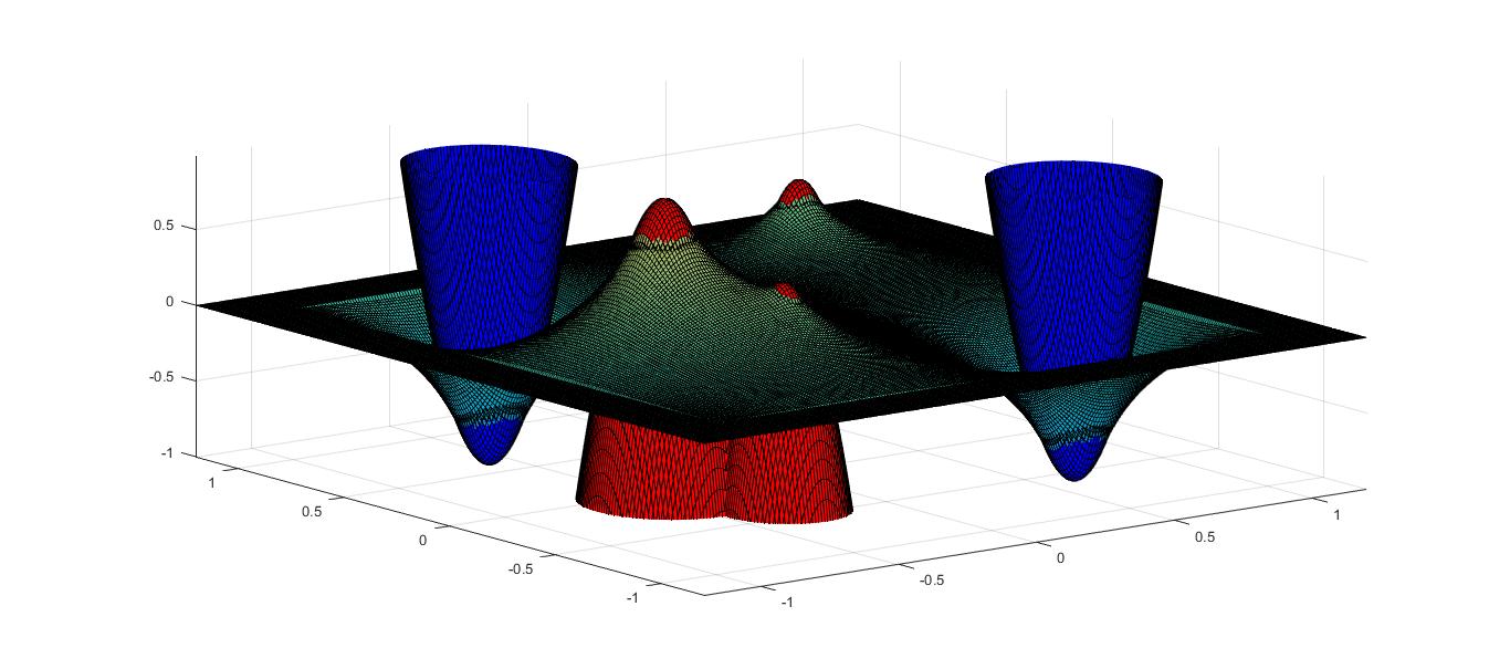
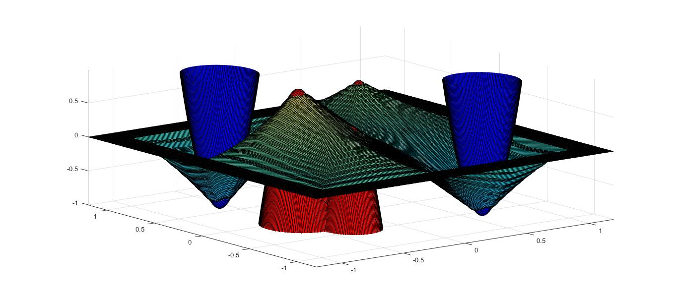
Figure 1. Results of tests for $p=2$ and $p=100$ with data in (6.2)

In Figure 2 we show the computed solutions for $p=10$ and the following sets of data:

(a) Smooth obstacles with parabolic boundary condition:

$$\begin{split}\Psi_{1}(x,y)&=\max\Big{\{}2-33(x+0.5)^{2}-27(y+0.1)^{2},~{}1.5-40(x+0.3)^{2}-34(y+0.4)^{2},\\ &\qquad\qquad\qquad~{}2.5-36(x-0.6)^{2}-51(y-0.7)^{2},~{}-3\Big{\}},\\ \Psi_{2}(x,y)&=\min\Big{\{}33(x+0.6)^{2}+27(y-0.6)^{2}-3,~{}33(x-0.6)^{2}+27(y+0.6)^{2}-3,~{}3\Big{\}},\\ F(x,y)&=1-2y^{2}.\end{split}$$

(b) Lipschitz obstacles with zero boundary condition:

$$\begin{split}\Psi_{1}(x,y)&=\begin{cases}2-17|x-0.5|&\quad\mbox{ for }y\in\left[-0.5,0.5\right]\\ 2-17|x-0.5|-17|y+0.5|&\quad\mbox{ for }y\in(-1,-0.5)\\ 2-17|x-0.5|-17|y-0.5|&\quad\mbox{ for }y\in(0.5,1)\end{cases}\\ \Psi_{2}(x,y)&=-4+12|y+0.2|+15|x-0.7|\\ F(x,y)&=0.\end{split}$$

(c) Smooth obstacles with hyperbolic boundary condition, where $\Psi_{1}$ and $\Psi_{2}$ are as in (a), and:

$$F(x,y)=2-(x+y)^{2}.$$

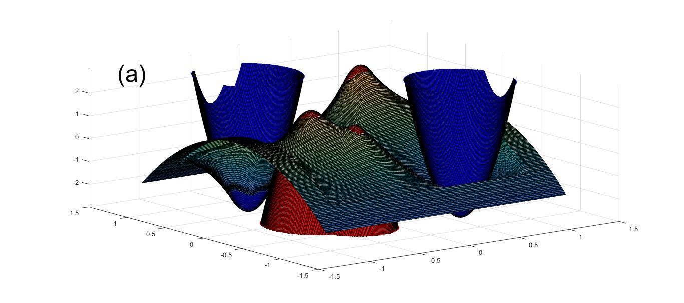
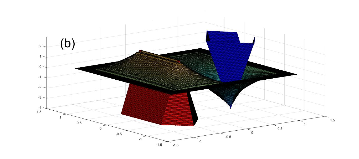
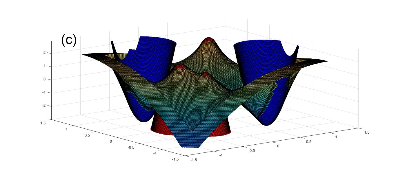
Figure 2. Results of tests for $p=10$ and data in (a), (b), (c), respectively.

The choice of radius and performance. We ran tests with the radius $\epsilon$ corresponding to $15$, $10$, $5$ and $3$ mesh size, for eighteen boundary conditions and obstacle functions. The table below gathers the information on the obtained execution time and precision. Runtime denotes the average time in seconds it took to run the experiments for a given radius. Iteration No denotes the number of times the operator $\bar{T}$ was applied before obtaining precision of less than $10^{-3}$. Error 1 is the error measured in the problem whose known solution is $e^{x}\sin(y)$ and $p=25$. Error 2 is the error measured in the problem whose solution is $x^{2}-y^{2}-y$ with no obstacles and $p=2$.

Radius	$k$ = Points Sampled	Runtime	Iteration No.	Error 1	Error 2
15	709	555	335	$8.62\cdot 10^{-6}$	$8.22\cdot 10^{-11}$
10	317	617	876	$6.17\cdot 10^{-6}$	$8.51\cdot 10^{-11}$
5	81	652	3361	$2.68\cdot 10^{-6}$	$8.68\cdot 10^{-11}$
3	29	540	9255	$3.15\cdot 10^{-7}$	$4.73\cdot 10^{-7}$

Next we look at how the algorithm performs for different values of $p$. We ran the algorithm with six different boundary conditions with no obstacle, one obstacle and two obstacles, each time for values $p=2,3,4,5,10,25,50,100$. The larger the value of $p$, the faster the algorithm converged as can be seen in the following table. Each row measures how many iterations it took for the algorithm to produce a precision of $10^{-3}$ on average over the six boundary conditions.

$p$	3	4	5	10	25	50	100
No Obstacle	5180	4806	4569	3790	3003	2707	209
One Obstacle	1637	1392	1249	975	825	777	166
Two Obstacles	1842	1933	1366	1108	992	967	178

References

- [1] C. Bjorland, L. Caffarelli and A. Figalli, Non-local tug-of-war and the infinity fractional Laplacian, Comm. Pure and Applied Math. 65, Issue 3, 337-–380 (2012).
- [2] G. Dal Maso, U. Mosco, and M. A. Vivaldi, M. A.,A pointwise regularity theory for the two-obstacle problem, Acta Math. 163, no. 1-2, 57–107, 1989
- [3] Z. Farnana, The double obstacle problem on metric spaces, Annales Acad. Sci. Fennicae Math. 34, 261–277 (2009).
- [4] P. Juutinen, P. Lindqvist and J. Manfredi, On the equivalence of viscosity solutions and weak solutions for a quasi-linear elliptic equation, SIAM J. Math. Anal. 33, 699–717 (2001).
- [5] T. Kilpeläinen and W. Ziemer, Pointwise regularity of solutions to nonlinear double obstacle problems, Ark. Mat. 29 (1), 83–106, 1991
- [6] M. Lewicka and J. Manfredi, The obstacle problem for the Laplacian via optimal stopping of tug-of-war games, to appear.
- [7] P. Lindqvist, On the definition and properties of -superharmonic functions, J. Reine Angew. Math. 365, 67–79 (1986).
- [8] H. Luiro, M. Parviainen, and E. Saksman, On the existence and uniqueness of p-harmonious functions, Differential and Integral Equations 27 201–216 (2014).
- [9] J. Manfredi, M. Parviainen, and J. Rossi, On the definition and properties of p-harmonious functions, Ann. Sc. Norm. Super. Pisa Cl. Sci. 11(2), 215–241, (2012).
- [10] J. Manfredi, J. Rossi and S. Somersille, An obstacle problem for Tug-of-War games, Communications on Pure and Applied Analysis. 14, 217–228, (2015).
- [11] A. Oberman, Finite difference methods for the Infinity Laplace and p-Laplace equations, Journal of Computational and Applied Math. 254, 65–80, (2013).
- [12] Y. Peres, O. Schramm, S. Sheffield and D. Wilson, Tug-of-war and the infinity Laplacian, J. Amer. Math. Soc. 22, 167–210 (2009).
- [13] Y. Peres, S. Sheffield, Tug-of-war with noise: a game theoretic view of the p-Laplacian, Duke Math. J. 145(1), 91–120, (2008).
- [14] M. Reppen and P. Moosavi, A review of the double obstacle problem, a degree project, KTH Stockholm (2011).
- [15] S. Varadhan, Probability theory, Courant Lecture Notes in Mathematics, 7.
- [16] F. Wang and X.L. Cheng, An algorithm for solving the double obstacle problems, Applied Math. and Computation 201, 221–228, (2008).