Light meson electromagnetic form factors from three-flavor lattice QCD with exact chiral symmetry

Abstract

We study the chiral behavior of the electromagnetic (EM) form factors of pion and kaon in three-flavor lattice QCD. In order to make a direct comparison of the lattice data with chiral perturbation theory (ChPT), we employ the overlap quark action that has exact chiral symmetry. Gauge ensembles are generated at a lattice spacing of 0.11 fm with four pion masses ranging between $M_{\pi}\simeq 290$ MeV and 540 MeV and with a strange quark mass $m_{s}$ close to its physical value. We utilize the all-to-all quark propagator technique to calculate the EM form factors with high precision. Their dependence on $m_{s}$ and on the momentum transfer is studied by using the reweighting technique and the twisted boundary conditions for the quark fields, respectively. A detailed comparison with SU(2) and SU(3) ChPT reveals that the next-to-next-to-leading order terms in the chiral expansion are important to describe the chiral behavior of the form factors in the pion mass range studied in this work. We estimate the relevant low-energy constants and the charge radii, and find reasonable agreement with phenomenological and experimental results.

I Introduction

Rapid increase of computational power and improvements of simulation algorithms allow us to perform large-scale simulations of unquenched lattice QCD in the chiral regime, where the non-perturbative dynamics is characterized by chiral symmetry. Chiral perturbation theory (ChPT) ChPT:SU2:NLO ; ChPT:SU3:NLO is an effective theory in this regime, though its Lagrangian has unknown parameters, called low-energy constants (LECs). A detailed comparison between lattice QCD and ChPT may validate numerical lattice calculations and analytical predictions of ChPT. This also provides a first-principle determination of LECs, and hence widens the applicability of ChPT to different physical observables.

In such a program, chiral symmetry plays an essential role. But, it is violated in most of the existing lattice calculations, and the comparison had to be made after carefully taking the continuum limit. Effects of the explicit violation by the use of conventional Wilson and staggered fermion formulations on the lattice were studied at next-to-leading order (NLO) in ChPT WChPT:SS ; SChPT:LS ; WChPT:RS ; SChPT:AB ; WChPT:A ; SChPT:SV : in general, it modifies the functional form of the ChPT expansion of physical observables, and introduces additional unknown LECs. It is therefore not clear how one can disentangle the next-to-next-to-leading order (NNLO) corrections, which are significant in kaon physics, from the extra terms due to the explicit chiral violation. Lattice QCD with exact chiral symmetry provides a clean framework for an unambiguous comparison between lattice QCD and ChPT. The JLQCD and TWQCD collaborations have performed such simulations employing the overlap quark action Overlap:NN ; Overlap:N , and studied the chiral behavior of various observables in detail JLQCD:overlap:summary .

Pion and kaon electromagnetic (EM) form factors are fundamental quantities in ChPT. The charged pion EM form factor $F_{V}^{\pi^{+}}$ is defined through the matrix element of the EM current $J_{\mu}$ sandwiched by the pion states

$$\langle P(p^{\prime})|J_{\mu}|P(p)\rangle = \left(p+p^{\prime}\right)_{\mu}F_{V}^{P}(t),\hskip 14.22636ptt=(p-p^{\prime})^{2},$$ (1)

$$J_{\mu} = \frac{2}{3}\bar{u}\gamma_{\mu}u-\frac{1}{3}\bar{d}\gamma_{\mu}d-\frac{1}{3}\bar{s}\gamma_{\mu}s,$$ (2)

where $|P(p)\rangle$ specifies the light meson state (charged pion $P\!=\!\pi^{+}$, to be explicit) of momentum $p$, and $t=(p-p^{\prime})^{2}$ is the momentum transfer. This form factor is known up to NNLO both in SU(2) ChPT ChPT:SU2:NLO ; PFF:ChPT:Nf2:NNLO:GM ; PFF:ChPT:SU2:NNLO:BCT , where the dependence on the strange quark mass $m_{s}$ is implicitly encoded in LECs, and in SU(3) ChPT with strange mesons as dynamical degrees of freedom PFF:ChPT:SU3:NLO ; PFF+KFF:ChPT:NNLO:Nf3 . Detailed analyses of experimental data based on NNLO ChPT have led to precise estimates of the charge radius PFF:ChPT:SU2:NNLO:BCT ; PFF+KFF:ChPT:NNLO:Nf3 ,

$${\langle r^{2}\rangle_{V}^{P}} = 6\left.\frac{\partial F_{V}^{P}(t)}{\partial t}\right|_{t=0},$$ (3)

which can be used as a benchmark of lattice calculations. Its dependence on the momentum transfer $t$ and mass of degenerate up and down quarks $m_{l}$ has been studied in unquenched lattice QCD PFF:Nf2:DBW2+DW:RBC ; PFF:Nf2:Plq+Clv:HKL ; PFF:Nf3:impG+AT+DWF:LHP ; PFF:Nf2:Plq+Clv:JLQCD ; PFF:Nf2:Plq+Clv:QCDSF ; PFF:Nf3:RG+DW:RBC+UKQCD ; PFF:Nf2:Sym+tmW:ETMC ; PFF:JLQCD:Nf2:RG+Ovr ; PFF:Nf3:RG+Clv:PACS-CS ; PFF:Nf2:impG+Clv:Mainz ; PFF:Nf3:impG+HISQ:HPQCD . Recent detailed comparisons with SU(2) ChPT PFF:Nf2:Sym+tmW:ETMC ; PFF:JLQCD:Nf2:RG+Ovr ; PFF:Nf3:RG+Clv:PACS-CS ; PFF:Nf2:impG+Clv:Mainz ; PFF:Nf3:impG+HISQ:HPQCD show that lattice data at the pion mass $M_{\pi}\!\lesssim\!500$ MeV are described reasonably well by the NNLO chiral expansion, and reproduce the experimental value of the pion charge radius. The NNLO contribution turns out to be non-negligible in accordance with the two-loop ChPT analysis PFF:ChPT:SU2:NNLO:BCT . This test has not yet been extended to SU(3) ChPT, in which the $m_{s}$ dependence of $F_{V}^{\pi^{+}}$ and ${\langle r^{2}\rangle_{V}^{\pi^{+}}}$ is explicitly taken into account.

The EM form factors of the charged and neutral kaons are similarly defined through Eq. (1) with $P\!=\!K^{+}$ and $K^{0}$, respectively. Since strange valence quarks are involved, we need SU(3) ChPT to describe their chiral behavior . These form factors are known up to NNLO PFF+KFF:ChPT:NNLO:Nf3 . The $m_{s}$ expansion is expected to have poorer convergence than that in terms of $m_{l}$ due to $m_{s}\!\gg\!m_{l}$. A detailed examination of the convergence and first-principle determination of relevant LECs are helpful for a better understanding of kaon physics: for instance, a phenomenologically important form factors of the $K\!\to\!\pi$ semileptonic decays share LECs with the EM form factors KFF:weak:ChPT:SU3:NNLO:PS ; KFF:weak:ChPT:SU3:NNLO:BT . There has been no lattice calculation nor detailed comparison with ChPT to our knowledge.

In the present work, we calculate the pion and kaon EM form factors in three-flavor lattice QCD. We employ the overlap quark action Overlap:NN ; Overlap:N to maintain exact chiral symmetry for a direct comparison of our lattice data with ChPT up to NNLO. The form factors are precisely calculated using the all-to-all quark propagator A2A:SESAM ; A2A:TrinLat . We also utilize the reweighting technique reweight:1 ; reweight:2 and the twisted boundary conditions TBC to study their dependence on $m_{s}$ and $t$, respectively. We compare their chiral behavior with NNLO SU(2) and SU(3) ChPT in detail, and present an estimate of the relevant LECs and charge radii. Our preliminary analysis has been reported in Ref. Lat10:JLQCD:Kaneko .

This paper is organized as follows. Section II introduces our method to generate the gauge ensembles and to calculate relevant light meson correlators. The EM form factors are extracted at the simulation points in Section III. We then study the chiral behavior of the form factors based on NNLO SU(2) and SU(3) ChPT in Sections IV and V, respectively. We summarize our conclusions in Section VI.

II Simulation method

II.1 Configuration generation

We simulate $N_{f}\!=\!2+1$ QCD, in which strange quark has a distinct mass from degenerate up and down quarks. We employ the Iwasaki gauge action Iwasaki and the overlap quark action Overlap:NN ; Overlap:N . The Dirac operator of the latter is given by

$$D(m_{q}) = \left(1-\frac{m_{q}}{2m_{0}}\right)D(0)+m_{q},$$ (4)

$$D(0) = m_{0}\left(1+\gamma_{5}\,{\rm sgn}\left[H_{\rm W}(-m_{0})\right]\right).$$ (5)

Here $m_{q}$ represents the quark mass, whereas $-m_{0}$ is the mass parameter of the Hermitian Wilson-Dirac operator $H_{W}$ appearing in the construction of the overlap fermion as a kernel. We set $m_{0}\!=\!1.6$ so that the overlap-Dirac operator $D(m_{q})$ has good locality Prod_Run:JLQCD:Nf2:RG+Ovr . This action exactly preserves chiral symmetry at finite lattice spacing lat_chial_sym . This enables us to directly compare the lattice results for the form factors at a finite lattice spacing with ChPT in the continuum limit, where the NNLO chiral expansion is available.

We introduce an auxiliary determinant exW:Vranas ; exW+extmW:JLQCD

$$\Delta_{\rm W} = \frac{\det[H_{\rm W}(-m_{0})^{2}]}{\det[H_{\rm W}(-m_{0})^{2}+\mu^{2}]}\hskip 14.22636pt(\mu=0.2)$$ (6)

into the Boltzmann weight in the generation of the gauge ensembles. This suppresses exact- and near-zero modes of $H_{\rm W}(-m_{0})$, and hence remarkably reduces the computational cost without changing the continuum limit of the theory. Another interesting property of $\Delta_{\rm W}$ is that the global topological charge $Q$ is unchanged during the update of the gauge fields with the Hybrid Monte Carlo (HMC) algorithm. In this study, we simulate trivial topological sector, $Q=0$. We note that local topological excitations are active, and the topological susceptibility is consistent with the ChPT expectation chi_t:JLQCD . The effect of the fixed global topology is a part of finite volume effect, which is suppressed by the inverse of the space-time volume fixed_Q:AFHO .

We set the gauge coupling $\beta\!=6/g^{2}\!=\!2.30$, where the lattice spacing determined from the $\Omega$ baryon mass is $a\!=\!0.112(1)$ fm. We perform simulations at four values of degenerate up and down quark mass $m_{l}$ that cover a range of $M_{\pi}\!\sim\!290$ – 540 MeV. The gauge ensembles are generated at a strange quark mass $m_{s}\!=\!0.080$, which is close to its physical value $m_{s,\rm phys}\!=\!0.081$. The EM form factors at a different value $m_{s}\!=\!0.060$ are calculated by the reweighting method reweight:1 ; reweight:2 .

We set a spatial lattice extent to $N_{s}\!=\!L/a\!=\!24$ at $m_{l}\!\leq\!0.025$ and to 16 at $m_{l}\!\geq\!0.035$ in order to control finite volume effects by satisfying a condition $M_{\pi}L\gtrsim 4$. The additional finite volume effect due to the fixed global topology turned out to be small in our previous study in $N_{f}\!=\!2$ QCD on similar or even smaller lattice volumes. The temporal lattice size is fixed to $N_{t}\!=\!T/a\!=\!48$. At each combination of $m_{l}$ and $m_{s}$, we generate 50 gauge configurations separated by 50 HMC trajectories. The statistical error quoted in this article is estimated by a single-elimination jackknife method. Our simulation parameters are summarized in Table 1.

Table 1: Simulation parameters. Meson masses, $M_{\pi}$ and $M_{K}$ are in units of MeV.

lattice	$m_{l}$	$m_{s}$	$M_{\pi}$	$M_{K}$	$\theta$
$16^{3}\!\times\!48$	0.050	0.080	540(4)	617(4)	0.00, 0.40, 0.96, 1.60
$16^{3}\!\times\!48$	0.035	0.080	453(4)	578(4)	0.00, 0.60, 1.28, 1.76
$24^{3}\!\times\!48$	0.025	0.080	379(2)	548(3)	0.00, 1.68, 2.64
$24^{3}\!\times\!48$	0.015	0.080	293(2)	518(3)	0.00, 1.68, 2.64
$16^{3}\!\times\!48$	0.050	0.060	540(4)	567(4)	0.00, 0.40, 0.96, 1.60
$16^{3}\!\times\!48$	0.035	0.060	451(7)	524(5)	0.00, 0.60, 1.28, 1.76
$24^{3}\!\times\!48$	0.025	0.060	378(7)	492(7)	0.00, 1.68, 2.64
$24^{3}\!\times\!48$	0.015	0.060	292(3)	459(4)	0.00, 1.68, 2.64

II.2 Calculation of meson correlators

We employ the all-to-all quark propagator A2A:SESAM ; A2A:TrinLat in order to improve statistical accuracy of the meson correlators. Let us consider an expansion of the quark propagator $D(m_{q})^{-1}$ in terms of the eigenmodes of the overlap operator $D(m_{q})$, where $m_{q}$ $(q=l,s)$ represents the valence quark mass. Light meson observables including the EM form factors are expected to large contributions from the low-lying modes. We calculate this important part by

$$\left\{D(m_{q})^{-1}\right\}_{\rm low}(x,y) = \sum_{k=1}^{N_{e}}\frac{1}{\lambda_{k}^{(q)}}u_{k}(x)u_{k}^{\dagger}(y),$$ (7)

where $\lambda_{k}^{(q)}$ represents the $k$-th lowest eigenvalue of $D(m_{q})$, and $u_{k}$ is the normalized eigenvector associated with $\lambda_{k}^{(q)}$. Note that the overlap action has advantages in solving the eigenvalue problem: i) the eigenvector does not depend on $m_{q}$, which only changes the normalization and the additive shift of $D$ (see Eq. (4)), and ii) the left and right eigenvectors are equal to each other, since $D$ is normal. We employ the implicitly restarted Lanczos algorithm to calculate the low-modes, the number of which is $N_{e}\!=\!240$ (160) on the $24^{3}\!\times\!48$ ($16^{3}\!\times\!48$) lattice.

The remaining contribution from higher eigenmodes is evaluated stochastically by the noise method noise with the dilution technique A2A:TrinLat . We prepare a complex $Z_{2}$ noise vector for each configuration, and split it into $N_{d}=3\times 4\times N_{t}/2$ vectors $\eta_{d}(x)(d\!=\!1,\ldots,N_{d})$, each of which has non-zero elements only for a single combination of color and spinor indices and at two consecutive time-slices. The high-mode contribution can be estimated as

$$\left\{D(m_{q})^{-1}\right\}_{\rm high}(x,y) = \sum_{d=1}^{N_{d}}x_{d}^{(q)}(x)\,\eta_{d}^{\dagger}(y)$$ (8)

by solving a linear equation for each diluted source

$$D(m_{q})\,x_{d}^{(q)}=P_{\rm high}\,\eta_{d}\hskip 14.22636pt(d=1,\ldots,N_{d}).\hskip 5.69054pt$$ (9)

Here $P_{\rm high}\!=\!1-P_{\rm low}$, and $P_{\rm low}\!=\!\sum_{k=1}^{N_{e}}u_{k}\,u_{k}^{\dagger}$ is the projector to the eigenspace spanned by the low-modes.

The typical size of the momentum transfer is $|t|\!\gtrsim\!(500~{}\mbox{MeV})^{2}$ on our lattice of size $L\sim 1.8$ – 2.7 fm, if we insert the meson momenta by using the Fourier transformation with the standard periodic boundary condition. Our previous study in two-flavor QCD PFF:JLQCD:Nf2:RG+Ovr suggested that the next-to-next-to-next-to-leading order (N³LO) correction to the pion form factor $F_{V}^{\pi^{+}}$ can be sizable in this region of $t$. In order to suppress such higher order contributions, which are not known in ChPT, we simulate near-zero momentum transfers $|t|\!\lesssim\!(300~{}\mbox{MeV})^{2}$ by employing the twisted boundary condition TBC for the valence quarks

$$q({\bf x}+L\hat{k},x_{4})=e^{i\theta}q({\bf x},x_{4}),\hskip 8.53581pt\bar{q}({\bf x}+L\hat{k},x_{4})=e^{-i\theta}\bar{q}({\bf x},x_{4})\hskip 14.22636pt(k=1,2,3),$$ (10)

where $\hat{k}$ is a unit vector in the $k$-th direction. We set a common twist angle $\theta$ in all three spatial directions for simplicity. This boundary condition induces a quark momentum of $p_{k}=\theta/L\leq 2\pi/L$. We choose the angles listed in Table 1, so that $|t|\lesssim(300~{}\mbox{MeV})^{2}$, where the N³LO correction to $F_{V}^{\pi^{+}}$ is expected to be insignificant.

We calculate the all-to-all quark propagator for each choice of $\theta$. By combining Eqs. (7) and (8), the all-to-all propagator can be expressed as

$$\left\{D(m_{q};\theta)^{-1}\right\}(x,y) = \sum_{k=1}^{N_{v}}v_{k,\theta}^{(q)}(x)\,w_{k,\theta}^{(q)\dagger}(y)\hskip 8.53581pt(q=l,s)$$ (11)

with the following two sets of vectors $v$ and $w$

$$\left\{v_{1,\theta}^{(q)},...,v_{N_{v},\theta}^{(q)}\right\} = \left\{\frac{u_{1,\theta}}{\lambda_{1,\theta}^{(q)}},\ldots,\frac{u_{N_{e},\theta}}{\lambda_{N_{e},\theta}^{(q)}},x_{1,\theta}^{(q)},\dots,x_{N_{d},\theta}^{(q)}\right\},$$ (12)

$$\left\{w_{1,\theta}^{(q)},...,w_{N_{v},\theta}^{(q)}\right\} = \left\{u_{1,\theta},\ldots,u_{N_{e},\theta},\eta_{1,\theta}^{(q)},\dots,\eta_{N_{d},\theta}^{(q)}\right\},$$ (13)

where $N_{v}=N_{e}+N_{d}$.

Meson two-point functions with a temporal separation $\Delta x_{4}$ and a spatial momentum ${\bf p}$ can be expressed as

$$C^{\pi}_{\phi\phi^{\prime}}({\Delta x_{4}};{\bf p}) = \frac{1}{N_{t}}\sum_{x_{4}=1}^{N_{t}}\sum_{{{\bf x}^{\prime}},{\bf x}}\langle{{\mathcal{O}}}_{\pi,\phi^{\prime}}({{\bf x}^{\prime}},x_{4}+{\Delta x_{4}}){{\mathcal{O}}}_{\pi,\phi}({\bf x},x_{4})^{\dagger}\rangle e^{-i{\bf p}({{\bf x}^{\prime}}-{\bf x})}$$ (14)

$$= \frac{1}{N_{t}}\sum_{x_{4}=1}^{N_{t}}\sum_{k,k^{\prime}=1}^{N_{v}}{{\mathcal{O}}}^{(l,l)}_{\gamma_{5},\phi^{\prime},kk^{\prime},\theta\theta^{\prime}}(x_{4}+{\Delta x_{4}})\,{{\mathcal{O}}}^{(l,l)}_{\gamma_{5},\phi,k^{\prime}k,\theta^{\prime}\theta}(x_{4}).$$

$$C^{K}_{\phi\phi^{\prime}}({\Delta x_{4}};{\bf p}) = \frac{1}{N_{t}}\sum_{x_{4}=1}^{N_{t}}\sum_{{\bf x},{{\bf x}^{\prime}}}\langle{{\mathcal{O}}}_{K,\phi^{\prime}}({{\bf x}^{\prime}},x_{4}+{\Delta x_{4}}){{\mathcal{O}}}_{K,\phi}({\bf x},x_{4})^{\dagger}\rangle e^{-i{\bf p}({{\bf x}^{\prime}}-{\bf x})}$$ (15)

$$= \frac{1}{N_{t}}\sum_{x_{4}=1}^{N_{t}}\sum_{k,k^{\prime}=1}^{N_{v}}{{\mathcal{O}}}^{(s,l)}_{\gamma_{5},\phi^{\prime},kk^{\prime},\theta\theta^{\prime}}(x_{4}+{\Delta x_{4}})\,{{\mathcal{O}}}^{(l,s)}_{\gamma_{5},\phi,k^{\prime}k,\theta^{\prime}\theta}(x_{4}),$$

where $p_{i}\!=\!(\theta^{\prime}-\theta)/L$ ($i=1,2,3$) represents the meson momentum induced by the twisted boundary conditions. Interpolating operators for $\pi^{+}$ and $K^{+}$ are given by

$${{\mathcal{O}}}_{\pi,\phi}({\bf x},t) = \sum_{{\bf r}}\phi(|{\bf r}|)\bar{d}({\bf x}+{\bf r},t)\gamma_{5}u({\bf x},t),$$ (16)

$${{\mathcal{O}}}_{K,\phi}({\bf x},t) = \sum_{{\bf r}}\phi(|{\bf r}|)\bar{s}({\bf x}+{\bf r},t)\gamma_{5}u({\bf x},t),\hskip 14.22636pt$$ (17)

where $\phi(|{\bf r}|)$ is a smearing function. Note that light quarks are degenerate and denoted by $l$ $(\!=\!u,d)$ in this paper. The quantity

$${{\mathcal{O}}}^{(q,q^{\prime})}_{\Gamma,\phi,kk^{\prime},\theta\theta^{\prime}}(x_{4}) = \sum_{{\bf x},{\bf r}}\phi({\bf r})\,w_{k,\theta}^{(q)\dagger}({\bf x}+{\bf r},x_{4})\,\Gamma\,v_{k^{\prime},\theta^{\prime}}^{(q^{\prime})}({\bf x},x_{4}),$$ (18)

can be considered as a smeared meson field constructed from the $v$ and $w$ vectors at a time-slice $x_{4}$. In this study, we employ the local and an exponential smearing functions, namely $\phi_{l}({\bf r})\!=\!\delta_{{\bf r},{\bf 0}}$ and $\phi_{s}({\bf r})\!=\!\exp[-0.4|{\bf r}|]$.

Three-point functions needed to calculate the EM form factors can be constructed in a similar way. For example, the kaon three-point function with the light-quark current $V^{(l)}_{\mu}=\bar{l}\gamma_{\mu}l$ is expressed as

$$C^{K}_{{V^{(l)}_{\mu}},\phi\phi^{\prime}}({\Delta x_{4}},{\Delta x_{4}^{\prime}};{\bf p},{\bf p}^{\prime})$$ (19)

$$= \frac{1}{N_{t}}\sum_{x_{4}=1}^{N_{t}}\sum_{{\bf x},{{\bf x}^{\prime}},{{\bf x}^{\prime\prime}}}\langle{{\mathcal{O}}}_{K,\phi^{\prime}}({{\bf x}^{\prime\prime}},x_{4}+{\Delta x_{4}}+{\Delta x_{4}^{\prime}})V_{\mu}^{(l)}({{\bf x}^{\prime}},x_{4}+{\Delta x_{4}}){{\mathcal{O}}}_{K,\phi}({\bf x},x_{4})^{\dagger}\rangle$$

$$\hskip 256.0748pt\times e^{-i{{\bf p}^{\prime}}({{\bf x}^{\prime\prime}}-{{\bf x}^{\prime}})}e^{-i{\bf p}({{\bf x}^{\prime}}-{\bf x})}$$

$$= \frac{1}{N_{t}}\sum_{x_{4}=1}^{N_{t}}\sum_{k,k^{\prime},k^{\prime\prime}=1}^{N_{v}}{{\mathcal{O}}}^{(s,l)}_{\gamma_{5},\phi^{\prime},k^{\prime\prime}k^{\prime},\theta^{\prime\prime}\theta^{\prime}}(x_{4}+{\Delta x_{4}}+{\Delta x_{4}^{\prime}})\,{{\mathcal{O}}}^{(l,l)}_{\gamma_{\mu},\phi_{l},k^{\prime}k,\theta^{\prime}\theta}(x_{4}+{\Delta x_{4}})$$

$$\hskip 256.0748pt\times{{\mathcal{O}}}^{(l,s)}_{\gamma_{5},\phi,kk^{\prime\prime},\theta\theta^{\prime\prime}}(x_{4}),$$

where ${\Delta x_{4}}$ (${\Delta x_{4}^{\prime}}$) represents the temporal separation between the vector current and meson source (sink) operator. The initial and final meson momenta are given by the twist angles as

$$p_{i}=\frac{\theta-\theta^{\prime\prime}}{L},\hskip 14.22636ptp^{\prime}_{i}=\frac{\theta^{\prime}-\theta^{\prime\prime}}{L}\hskip 14.22636pt(i=1,2,3).$$ (20)

Note that we need to apply different twist angles to the quark and anti-quark fields in ${\cal O}_{P,\phi}$ and $V_{\mu}^{(q)}$ so that the mesons can carry non-zero momentum.

We only calculate connected diagrams because of the use of the twisted boundary condition. The contribution of the disconnected diagram to $F_{V}^{\pi^{+}}$ vanishes due to charge conjugation symmetry disconnected . As a numerical check, we calculate the disconnected contributions to $F_{V}^{\{\pi^{+},K^{+},K^{0}\}}$ with meson momenta ${\bf p}\!=\!(2\pi/L,0,0)$ and ${{\bf p}^{\prime}}\!=\!(0,0,0)$ using the Fourier transformation and the periodic boundary condition also for the valence quarks. The disconnected contributions turn out to be insignificant with our statistical accuracy.

By using the all-to-all propagator, we can average the meson correlators over the location of the source operator, i.e. the summation over ${\bf x}$ and $x_{4}$ in Eqs. (14), (15) and (19). Figure 1 compares the statistical fluctuation of the pion three-point function with a certain choice of ${\Delta x_{4}}^{(\prime)}$ and ${\bf p}^{(\prime)}$. We observe that an average over the temporal coordinate $x_{4}$ reduces the statistical error of the pion (kaon) three-point functions by about a factor of two (four).

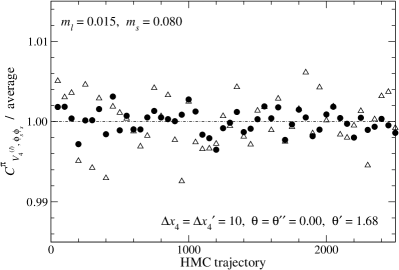
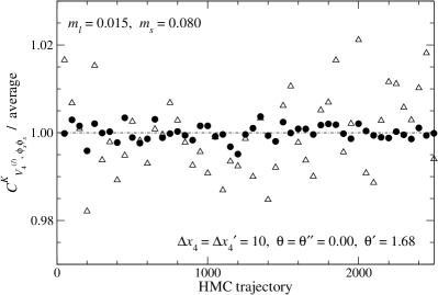
Figure 1: Statistical fluctuation of three-point functions, $C^{\pi}_{V_{4}^{(l)},\phi_{s}\phi_{s}}({\Delta x_{4}},{\Delta x_{4}^{\prime}};{\bf p},{{\bf p}^{\prime}})$ (left panel) and $C^{K}_{V_{4}^{(l)},\phi_{s}\phi_{s}}({\Delta x_{4}},{\Delta x_{4}^{\prime}};{\bf p},{{\bf p}^{\prime}})$ (right panel), with ${\Delta x_{4}}\!=\!{\Delta x_{4}^{\prime}}\!=\!10$, $\theta\!=\!\theta^{\prime\prime}\!=\!0.00$, $\theta^{\prime}\!=\!1.68$ at $(m_{l},m_{s})\!=\!(0.015,0.080)$. We plot the value at each jackknife sample normalized by the statistical average. Triangles and circles are data before and after averaging over the temporal location of the source operator $x_{4}$.

II.3 Reweighting

We use the gauge ensembles generated at the single value of $m_{s}\!=\!0.080$. In order to study the $m_{s}$ dependence of the EM form factors, the meson correlators are calculated at a different value $m_{s}^{\prime}\!=\!0.060$ by utilizing the reweighing technique reweight:1 ; reweight:2 . The kaon three-point function at $m_{s}^{\prime}$ is estimated on the gauge configurations at $m_{s}$ as

$$\langle C^{K}_{V_{\mu}^{(l)},\,\phi\phi^{\prime}}\rangle_{m_{s}^{\prime}} = \langle C^{K}_{V_{\mu}^{(l)},\,\phi\phi^{\prime}}\,\tilde{w}(m_{s}^{\prime},m_{s})\rangle_{m_{s}},$$ (21)

where $\langle\cdots\rangle_{m_{s}}$ represents the Monte Carlo average at $m_{s}$, and $\tilde{w}$ is the reweighting factor for each configuration

$$\tilde{w}(m_{s}^{\prime},m_{s}) = \frac{w(m_{s}^{\prime},m_{s})}{\langle w(m_{s}^{\prime},m_{s})\rangle_{m_{s}}},\hskip 14.22636ptw(m_{s}^{\prime},m_{s})=\det\left[\frac{D(m_{s}^{\prime})}{D(m_{s})}\right].$$ (22)

It is prohibitively time consuming to exactly calculate the quark determinant $\det[D(m_{s}^{(\prime)})]$. Instead, we decompose $w$ into contributions from low- and high-modes

$$w(m_{s}^{\prime},m_{s}) = w_{\rm low}(m_{s}^{\prime},m_{s})\,w_{\rm high}(m_{s}^{\prime},m_{s}),$$ (23)

$$w_{\rm low(high)}(m_{s}^{\prime},m_{s}) = \det\left[P_{\rm low(high)}\frac{D(m_{s}^{\prime})}{D(m_{s})}P_{\rm low(high)}\right],$$ (24)

and the low mode contribution $w_{\rm low}$ is exactly calculated by using the low-lying eigenvalues. We estimate the high-mode contribution $w_{\rm high}$ by a stochastic estimator for

$$w_{\rm{high}}^{2}(m_{s}^{\prime},m_{s})=\frac{1}{N_{r}}\sum_{r=1}^{N_{r}}e^{-\frac{1}{2}(P_{\rm high}\xi_{r})^{\dagger}(\Omega-1)P_{\rm high}\xi_{r}},$$ (25)

with $\Omega\equiv D(m_{s})^{\dagger}\{D(m_{s}^{\prime})^{-1}\}^{\dagger}D(m_{s}^{\prime})^{-1}D(m_{s})$. We introduce $N_{r}$ normalized Gaussian random vectors $\{\xi_{1},...,\xi_{N_{r}}\}$.

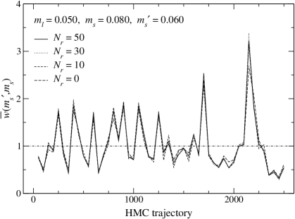
Figure 2: Monte Carlo history of reweighting factor $\tilde{w}(m_{s}^{\prime},m_{s})$ at $m_{l}\!=\!0.050$ with different numbers of the Gaussian random vector $N_{r}$.

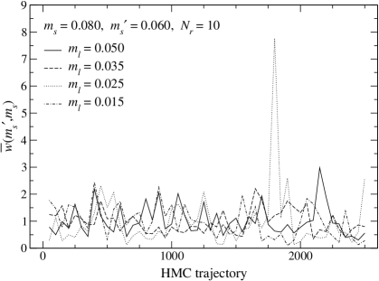
Figure 3: Monte Carlo history of reweighting factor $\tilde{w}(m_{s}^{\prime},m_{s})$ calculated with $N_{r}\!=\!10$. Different lines show data at different $m_{l}$.

At $m_{l}\!=\!0.050$, we study how many Gaussian random vectors are needed to reliably estimate the high-mode contribution $w_{\rm{high}}$ for the reweighting from $m_{s}\!=\!0.080$ to $m_{s}^{\prime}\!=\!0.060$. The normalized reweighting factor $\tilde{w}$ shows rather minor dependence on $N_{r}$, as shown in Fig. 2. This suggests that $\tilde{w}$ is dominated by the low-mode contribution $w_{\rm low}$ for our choice of the number of low-modes $N_{e}$ and the lattice size $N_{s}^{3}\times N_{t}$. We do not need many random vectors and set $N_{r}\!=\!10$ in this study.

Figure 3 compares $\tilde{w}$ at different values of $m_{l}$. We observe that $\tilde{w}$ is typically in a range [0.5, 2.0]. There is no systematic trend in the magnitude of the statistical fluctuation of $\tilde{w}$, as we decrease $m_{l}$. We therefore consider that a large value $\tilde{w}\simeq 8$ observed at $m_{l}\!=\!0.025$ and at 1800-th HMC trajectory is accidental.

III EM form factors and charge radii at simulation points

III.1 EM form factors

Two- and three-point functions of the light mesons ($P\!=\!\pi,K$) are dominated by the ground state contribution

$$C^{P}_{\phi\phi^{\prime}}({\Delta x_{4}};{\bf p}) \xrightarrow[{\Delta x_{4}}\to\infty]{} \frac{Z_{P,\phi^{\prime}}({\bf p})^{*}\,Z_{P,\phi}({\bf p})}{2\,E_{P}({\bf p})}\,e^{-E_{P}({\bf p})\,{\Delta x_{4}}},$$ (26)

$$C^{P}_{J_{\mu},\phi\phi^{\prime}}({\Delta x_{4}},{\Delta x_{4}^{\prime}};{\bf p},{{\bf p}^{\prime}}) \xrightarrow[{\Delta x_{4}},{\Delta x_{4}^{\prime}}\to\infty]{} \frac{Z_{P,\phi^{\prime}}({{\bf p}^{\prime}})^{*}\,Z_{P,\phi}({\bf p})}{4\,E_{P}({{\bf p}^{\prime}})E_{P}({\bf p})}\frac{1}{Z_{V}}\langle P(p^{\prime})|J_{\mu}|P(p)\rangle\,$$ (27)

$$\hskip 71.13188pt\times e^{-E_{P}({{\bf p}^{\prime}})\,{\Delta x_{4}^{\prime}}}e^{-E_{P}({\bf p})\,{\Delta x_{4}}},$$

in the limit of large temporal separations between the meson source/sink operators and the EM current ${\Delta x_{4}},{\Delta x_{4}^{\prime}}\!\to\!\infty$. Here $Z_{V}$ is the renormalization factor for the vector current, and $Z_{P,\phi}({\bf p})\!=\!\langle P(p)|{{\mathcal{O}}}_{P,\phi}\rangle$ is the overlap of the meson interpolating field to the physical state. We consider a ratio

$$R_{V}^{PQ}({\Delta x_{4}},{\Delta x_{4}^{\prime}};{\bf p},{\bf p}^{\prime}) = \frac{C^{P}_{J_{4},\phi_{s}\phi_{s}}({\Delta x_{4}},{\Delta x_{4}^{\prime}};{\bf p},{{\bf p}^{\prime}})\,C^{Q}_{\phi_{s}\phi_{l}}({\Delta x_{4}};{\bf 0})\,C^{Q}_{\phi_{l}\phi_{s}}({\Delta x_{4}^{\prime}};{\bf 0})}{C^{Q}_{J_{4},\phi_{s}\phi_{s}}({\Delta x_{4}},{\Delta x_{4}^{\prime}};{\bf 0},{\bf 0})\,C^{P}_{\phi_{s}\phi_{l}}({\Delta x_{4}};{\bf p})\,C^{P}_{\phi_{l}\phi_{s}}({\Delta x_{4}^{\prime}};{{\bf p}^{\prime}})},$$ (28)

with three choices of $(P,Q)\!=\!(\pi^{+},\pi^{+})$, $(K^{+},K^{+})$ and $(K^{0},K^{+})$. Since $Z_{K^{+},\phi}\!=\!Z_{K^{0},\phi}$ with our simulation setup $m_{u}\!=\!m_{d}$, normalization factors $Z_{P,\phi_{\{l,s\}}}$ and $Z_{V}$ as well as the exponential damping factors $e^{-E_{P}({\bf p}^{(\prime)}){\Delta x_{4}}^{(\prime)}}$ cancel in the ratio, provided that they are dominated by the ground state contribution dble_ratio . Therefore we can calculate the effective value of the EM form factors through this ratio as

$$F_{V}^{P}({\Delta x_{4}},{\Delta x_{4}^{\prime}};t) = \frac{F_{V}^{P}({\Delta x_{4}},{\Delta x_{4}^{\prime}};t)}{F_{V}^{Q}({\Delta x_{4}},{\Delta x_{4}^{\prime}};0)}=\frac{2\,M_{Q}}{E_{P}({\bf p})+E_{P}({{\bf p}^{\prime}})}R_{V}^{PQ}({\Delta x_{4}},{\Delta x_{4}^{\prime}};{\bf p},{\bf p}^{\prime}),$$ (29)

where we assume the vector current conservation $F_{V}^{Q}(0)\!=\!1$ ($Q\!=\!\pi^{+},K^{+}$), and use $M_{P}$ and $E_{P}$ determined by fitting two-point functions to Eq. (26).

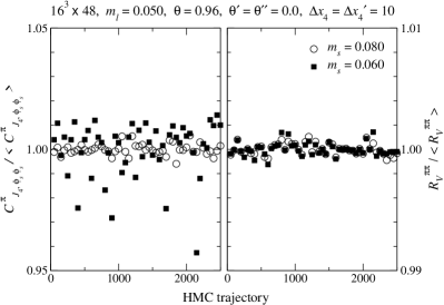
Figure 4: Pion three-point function $C^{\pi}_{J_{4},\phi_{s}\phi_{s}}({\Delta x_{4}},{\Delta x_{4}^{\prime}};{\bf p},{{\bf p}^{\prime}})$ (left panel) and ratio $R_{V}^{\pi\pi}({\Delta x_{4}},{\Delta x_{4}^{\prime}};{\bf p},{{\bf p}^{\prime}})$ (right panel) at each jackknife sample. We plot data, which are normalized by their statistical average, at $m_{l}\!=\!0.050$, $\theta\!=\!0.96$, $\theta^{\prime}\!=\!\theta^{\prime\prime}\!=\!0.0$ and ${\Delta x_{4}}\!=\!{\Delta x_{4}^{\prime}}\!=\!10$. Circles and squares are data before ($m_{s}\!=\!0.080$) and after ($m_{s}\!=\!0.060$) reweighting. The horizontal axis represents the HMC trajectory count of the excluded configuration for the jackknife analysis. Note that the scale is much finer for the right panel than the left.

Taking the ratio $R_{V}^{PQ}$ turns out to be effective also in reducing statistical fluctuation induced by reweighting. The reweighting factor in our study is typically in a region $\tilde{w}\!\in\![0.5,2.0]$, and significantly enhances the statistical fluctuation of the meson correlators. In Fig. 4, for instance, we observe about a factor of 5 increase in the statistical error of the pion three-point function $C^{\pi}_{J_{4},\phi_{s}\phi_{s}}$ at $m_{l}\!=\!0.050$. The enhanced fluctuation, however, largely cancels in the ratio $R_{V}^{PQ}$, whose error increases only by $\approx$ 15 % by reweighting. This is also the case at $m_{l}\!=\!0.025$, where the reweighing factor in Fig. 3 takes occasionally a rather large value $\tilde{w}\!\simeq\!8$. As suggested in Fig. 5, the reweighting increases the error of $C^{\pi}_{J_{4},\phi_{s}\phi_{s}}$ by about a factor of 24, which is however remarkably reduced to 1.6 in the ratio $R_{V}^{PQ}$.

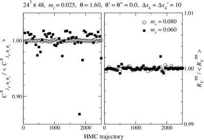
Figure 5: Same as Fig. 4, but for $m_{l}\!=\!0.025$. Note that the large value $\tilde{w}\!\sim\!8$ in Fig. 3 leads to a small (large) value of the three-point function (the ratio $R_{V}^{\pi\pi}$) at 1800th trajectory.

We extract the EM form factor $F_{V}^{P}(t)$ by a constant fit to the effective value $F_{V}^{P}({\Delta x_{4}},{\Delta x_{4}^{\prime}};t)$. Figures 6 – 11 show examples of this fit for $F_{V}^{\pi^{+}}$ (Figs. 6 – 7), $F_{V}^{K^{+}}$ (Figs. 8 – 9), and $F_{V}^{K^{0}}$ (Figs. 10 – 11). We summarize numerical results in Tables 2 – 9.

The charged meson form factors are the sum of the contributions with the light and strange quark currents

$$F_{V}^{\pi^{+}} \propto \frac{2}{3}\langle\pi\left|\bar{u}\gamma_{\mu}u\right|\pi\rangle+\frac{1}{3}\langle\pi\left|\bar{d}\gamma_{\mu}d\right|\pi\rangle=\langle\pi\left|\bar{l}\gamma_{\mu}l\right|\pi\rangle,$$ (30)

$$F_{V}^{K^{+}} \propto \frac{2}{3}\langle K^{+}\left|\bar{u}\gamma_{\mu}u\right|K^{+}\rangle+\frac{1}{3}\langle K^{+}\left|\bar{s}\gamma_{\mu}s\right|K^{+}\rangle$$ (31)

$$= \frac{2}{3}\langle K^{+}\left|\bar{l}\gamma_{\mu}l\right|K^{+}\rangle+\frac{1}{3}\langle K^{+}\left|\bar{s}\gamma_{\mu}s\right|K^{+}\rangle.$$

Their normalizations are fixed as $F_{V}^{P}(0)\!=\!1$ ($P\!=\!\pi^{+},K^{+}$) from the vector current conservation. Equation (29) implies that what we study using $R_{V}^{PP}$ is a ratio $F_{V}^{P}(t)/F_{V}^{P}(0)$, namely the finite $t$ correction to $F_{V}^{P}(t)$. Since we explore near-zero momentum transfer $t\!\sim\!0$, this correction is not large: typically $F_{V}^{P}(0)-F_{V}^{P}(t)\lesssim 0.1$ as seen in Tables 2 – 9. Its statistical accuracy is typically 5 % at $m_{s}\!=\!0.080$ and 10 % at $m_{s}\!=\!0.060$. For these fitted values of $F_{V}^{P}$, we observe about a factor of two larger error after the reweighting from $m_{s}\!=\!0.080$ to 0.060.

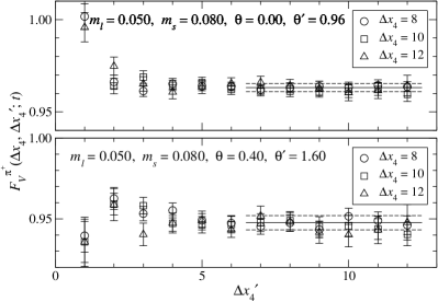
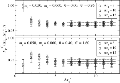
Figure 6: Effective value of pion EM form factor $F_{V}^{\pi^{+}}({\Delta x_{4}},{\Delta x_{4}^{\prime}},t)$ at $m_{l}=0.050$. Left and right panels show data at $m_{s}\!=\!0.080$ and 0.060, whereas top and bottom panels are with $(\theta,\theta^{\prime},\theta^{\prime\prime})\!=\!(0.00,0.96,0.00)$ and $(0.40,1.60,0.00)$.

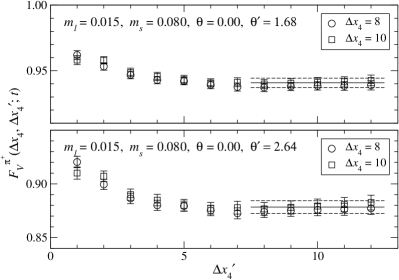
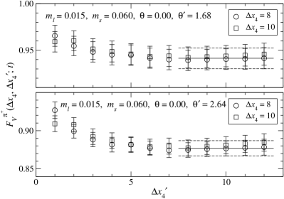
Figure 7: Effective value of pion EM form factor $F_{V}^{\pi^{+}}({\Delta x_{4}},{\Delta x_{4}^{\prime}},t)$ at $m_{l}=0.015$. Left and right panels show data at $m_{s}\!=\!0.080$ and 0.060, whereas top and bottom panels are with $(\theta,\theta^{\prime},\theta^{\prime\prime})\!=\!(0.00,1.68,0.00)$ and $(0.00,2.64,0.00)$.

ChPT suggests that finite volume effects are exponentially suppressed as $\propto\!\exp[-M_{\pi}L]$ FVE:ChPT:TBC:GS , which is roughly 2 % or less on the lattices with $M_{\pi}L\!\gtrsim\!4$. It is recently argued in Ref. FVE:ChPT:TBC:BR that the twisted boundary condition breaks reflection symmetry and gives rise to an additional correction, which is at the level of 0.1 % for meson masses and decay constants at $M_{\pi}L\!\sim\!4$. These effects are well below the accuracy of the finite $t$ correction to $F_{V}^{P}$. Yet another finite volume correction appears in our simulations due to the fixed global topology. We expect from our previous study on a similar volume PFF:JLQCD:Nf2:RG+Ovr that this effect is also small compared to the statistical accuracy.

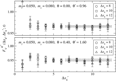
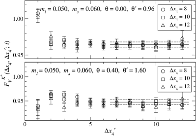
Figure 8: Effective value of charged kaon EM form factor $F_{V}^{K^{+}}({\Delta x_{4}},{\Delta x_{4}^{\prime}},t)$ at $m_{l}\!=\!0.050$.

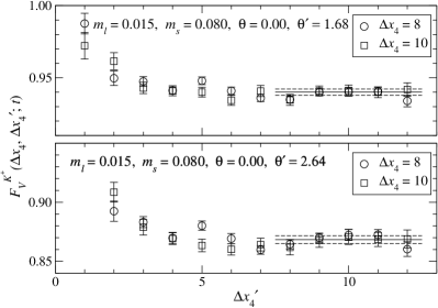
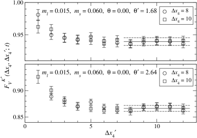
Figure 9: Effective value of charged kaon EM form factor $F_{V}^{K^{+}}({\Delta x_{4}},{\Delta x_{4}^{\prime}},t)$ at $m_{l}\!=\!0.015$.

The neutral kaon form factor is the difference between the contributions of the light and strange quark currents

$$F_{V}^{K^{0}} \propto -\frac{1}{3}\langle\pi\left|\bar{l}\gamma_{\mu}l\right|\pi\rangle+\frac{1}{3}\langle\pi\left|\bar{s}\gamma_{\mu}s\right|\pi\rangle,$$ (32)

which vanishes at $t\!=\!0$. In the region of small $|t|$, $F_{V}^{K^{0}}(t)$ is close to zero as seen in Figs. 10 and 11. The use of the all-to-all quark propagator enables us to calculate this small form factor with an error of $\gtrsim\!15$ %. The above mentioned finite volume corrections are negligible at this level of uncertainties.

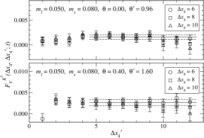
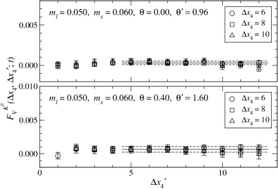
Figure 10: Effective value of neutral kaon EM form factor $F_{V}^{K^{0}}({\Delta x_{4}},{\Delta x_{4}^{\prime}},t)$ at $m_{l}\!=\!0.050$.

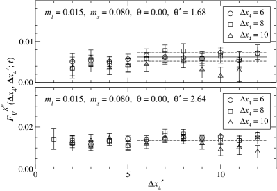
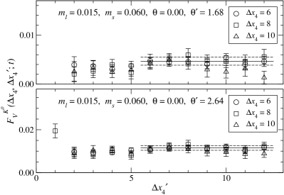
Figure 11: Effective value of neutral kaon EM form factor $F_{V}^{K^{0}}({\Delta x_{4}},{\Delta x_{4}^{\prime}},t)$ at $m_{l}\!=\!0.015$.

Table 2: Fit results for EM form factors at $(m_{l},m_{s})\!=\!(0.050,0.080)$.

$\theta$	$\theta^{\prime}$	$\theta^{\prime\prime}$	$F_{V}^{\pi^{+}}(t)$	$F_{V}^{K^{+}}(t)$	$F_{V}^{K^{0}}(t)$
0.00	0.40	0.00	0.9936(13)	0.9944(13)	0.00029(27)
0.00	0.96	0.00	0.9632(22)	0.9659(21)	0.00157(47)
0.00	1.60	0.00	0.9082(29)	0.9114(32)	0.00426(58)
0.40	0.96	0.00	0.9875(33)	0.9900(29)	0.00044(64)
0.40	1.60	0.00	0.9476(44)	0.9508(36)	0.00267(73)
0.96	1.60	0.00	0.9837(66)	0.9870(54)	0.0009(10)

Table 3: Fit results for EM form factors at $(m_{l},m_{s})\!=\!(0.050,0.060)$.

$\theta$	$\theta^{\prime}$	$\theta^{\prime\prime}$	$F_{V}^{\pi^{+}}(t)$	$F_{V}^{K^{+}}(t)$	$F_{V}^{K^{0}}(t)$
0.00	0.40	0.00	0.9936(24)	0.9939(28)	-0.00006(12)
0.00	0.96	0.00	0.9634(30)	0.9645(36)	0.00031(22)
0.00	1.60	0.00	0.9071(46)	0.9089(39)	0.00130(31)
0.40	0.96	0.00	0.9878(42)	0.9888(52)	-0.00016(34)
0.40	1.60	0.00	0.9472(46)	0.9477(50)	0.00067(42)
0.96	1.60	0.00	0.9823(61)	0.9830(78)	-0.00004(61)

Table 4: Fit results for EM form factors at $(m_{l},m_{s})\!=\!(0.035,0.080)$.

$\theta$	$\theta^{\prime}$	$\theta^{\prime\prime}$	$F_{V}^{\pi^{+}}(t)$	$F_{V}^{K^{+}}(t)$	$F_{V}^{K^{0}}(t)$
0.00	0.60	0.00	0.9793(25)	0.9821(20)	0.00020(60)
0.00	1.28	0.00	0.9244(54)	0.9302(41)	0.00288(80)
0.00	1.76	0.00	0.8735(65)	0.8791(57)	0.00617(91)
0.60	1.28	0.00	0.9666(76)	0.9712(61)	-0.0017(22)
0.60	1.76	0.00	0.9318(85)	0.9375(74)	0.0007(15)
1.28	1.76	0.00	0.9627(19)	0.971(11)	-0.0032(31)

Table 5: Fit results for EM form factors at $(m_{l},m_{s})\!=\!(0.035,0.060)$.

$\theta$	$\theta^{\prime}$	$\theta^{\prime\prime}$	$F_{V}^{\pi^{+}}(t)$	$F_{V}^{K^{+}}(t)$	$F_{V}^{K^{0}}(t)$
0.00	0.60	0.00	0.9805(34)	0.9794(42)	-0.00032(44)
0.00	1.28	0.00	0.9235(68)	0.9232(55)	0.00128(49)
0.00	1.76	0.00	0.8717(87)	0.8711(70)	0.00266(71)
0.60	1.28	0.00	0.9661(90)	0.9695(81)	-0.0016(18)
0.60	1.76	0.00	0.929(11)	0.9287(92)	-0.0002(15)
1.28	1.76	0.00	0.957(21)	0.965(12)	-0.0022(16)

Table 6: Fit results for EM form factors at $(m_{l},m_{s})\!=\!(0.025,0.080)$.

$\theta$	$\theta^{\prime}$	$\theta^{\prime\prime}$	$F_{V}^{\pi^{+}}(t)$	$F_{V}^{K^{+}}(t)$	$F_{V}^{K^{0}}(t)$
0.00	1.68	0.00	0.9432(20)	0.9435(14)	0.00574(50)
0.00	2.64	0.00	0.8777(34)	0.8748(23)	0.01219(94)
1.68	2.64	0.00	0.9934(77)	0.9799(37)	0.00197(82)

Table 7: Fit results for EM form factors at $(m_{l},m_{s})\!=\!(0.025,0.060)$.

$\theta$	$\theta^{\prime}$	$\theta^{\prime\prime}$	$F_{V}^{\pi^{+}}(t)$	$F_{V}^{K^{+}}(t)$	$F_{V}^{K^{0}}(t)$
0.00	1.68	0.00	0.9398(95)	0.9400(75)	0.00426(42)
0.00	2.64	0.00	0.874(13)	0.8715(85)	0.00828(53)
1.68	2.64	0.00	0.992(20)	0.983(15)	0.00178(66)

Table 8: Fit results for EM form factors at $(m_{l},m_{s})\!=\!(0.015,0.080)$.

$\theta$	$\theta^{\prime}$	$\theta^{\prime\prime}$	$F_{V}^{\pi^{+}}(t)$	$F_{V}^{K^{+}}(t)$	$F_{V}^{K^{0}}(t)$
0.00	1.68	0.00	0.9407(35)	0.9400(22)	0.0062(10)
0.00	2.64	0.00	0.8784(60)	0.8684(33)	0.0149(13)
1.68	2.64	0.00	0.995(12)	0.9790(62)	0.0020(24)

Table 9: Fit results for EM form factors at $(m_{l},m_{s})\!=\!(0.015,0.060)$.

$\theta$	$\theta^{\prime}$	$\theta^{\prime\prime}$	$F_{V}^{\pi^{+}}(t)$	$F_{V}^{K^{+}}(t)$	$F_{V}^{K^{0}}(t)$
0.00	1.68	0.00	0.941(11)	0.9396(60)	0.00467(81)
0.00	2.64	0.00	0.877(10)	0.8664(56)	0.0115(11)
1.68	2.64	0.00	0.997(22)	0.985(11)	0.0001(20)

III.2 charge radii

In this article, we determine the charge radii ${\langle r^{2}\rangle_{V}^{P}}$ of the light mesons ($P\!=\!\pi^{+},K^{+},K^{0}$) at the physical quark masses from ChPT-based parametrizations of $F_{V}^{P}$. In this subsection, we assume a $t$ dependence of $F_{V}^{P}$ based on phenomenological models, and estimate the radii at simulated quark masses.

Figures 12 – 14 show the results for $F_{V}^{P}(t)$ as a function of the momentum transfer $t$. We observe that their $t$ dependence is reasonably well described by the vector meson dominance (VMD) hypothesis (in the plots shown by dot-dashed curves)

$$F_{V}^{\pi^{+}}(t) = \frac{1}{1-t/M_{\rho}^{2}},$$ (33)

$$F_{V}^{K^{+}}(t) = \frac{2}{3}\frac{1}{1-t/M_{\rho}^{2}}+\frac{1}{3}\frac{1}{1-t/M_{\phi}^{2}},$$ (34)

$$F_{V}^{K^{0}}(t) = -\frac{1}{3}\frac{1}{1-t/M_{\rho}^{2}}+\frac{1}{3}\frac{1}{1-t/M_{\phi}^{2}},$$ (35)

where $M_{\rho}$ and $M_{\phi}$ represent the light and strange vector meson masses calculated at the simulated quark masses. The small deviation may be attributed to the effects of higher poles and cuts, and is approximated by a polynomial correction in the following analysis. Because quadratic and higher order corrections turn out to be insignificant in the region of small $t$, we employ the following fitting forms

$$F_{V}^{\pi^{+}}(t) = \frac{1}{1-t/M_{\rho}^{2}}+a_{\pi}t,$$ (36)

$$F_{V}^{K^{+}}(t) = \frac{2}{3}\frac{1}{1-t/M_{\rho}^{2}}+\frac{1}{3}\frac{1}{1-t/M_{\phi}^{2}}+a_{K^{+}}t,$$ (37)

$$F_{V}^{K^{0}}(t) = -\frac{1}{3}\frac{1}{1-t/M_{\rho}^{2}}+\frac{1}{3}\frac{1}{1-t/M_{\phi}^{2}}+a_{K^{0}}t$$ (38)

to estimate the charge radii defined in Eq. (3). We also carry out linear and quadratic fits

$$F_{V}^{P}(t) = b_{0}^{P}+b_{1}^{P}t\ (+b_{2}^{P}t^{2})$$ (39)

with $b_{0}^{\pi^{+}}=b_{0}^{K^{+}}=1$ and $b_{0}^{K^{0}}=0$. The systematic uncertainty due to the choice of the parametrization form (36) – (38) is estimated by the difference in ${\langle r^{2}\rangle_{V}^{P}}$ from these polynomial fits.

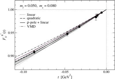
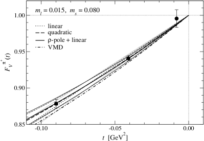
Figure 12: Pion EM form factor $F_{V}^{\pi^{+}}(t)$ as a function of momentum transfer $t$. The left and right panels show data at $(m_{l},m_{s})\!=\!(0.050,0.080)$ and (0.015,0.080), respectively. Thick dotted and dashed lines show linear and quadratic fits, whereas the fit based on VMD is plotted by the thick solid line. Their errors are plotted by thin lines. The thick dot-dashed line shows the $t$ dependence expected from VMD.

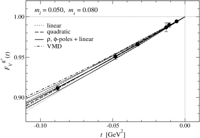
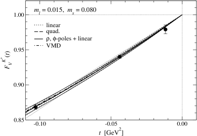
Figure 13: Charged kaon EM form factor $F_{V}^{K^{+}}(t)$ as a function of momentum transfer $t$.

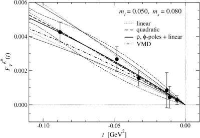
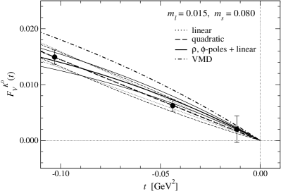
Figure 14: Neutral kaon EM form factor $F_{V}^{K^{0}}(t)$ as a function of momentum transfer $t$.

In Figs 12 – 14, we also plot fit curves with these parametrizations. Numerical results for ${\langle r^{2}\rangle_{V}^{P}}$ are summarized in Table 10. The radii have larger systematic error on the larger lattice, namely at $m_{l}\!\leq\!0.025$, simply because we simulate only three values of $t$ in order to reduce the computational cost. At each simulation point, our data favor a smaller radius for the heavier charged meson $K^{+}$ than for the lighter one $\pi^{+}$, though the difference is not large. The radius of the neutral meson $K^{0}$ is much smaller than those for the charged mesons. (Notice the scale of the vertical axis in Fig. 14.) These are qualitatively in accordance with ChPT and experiments. We give quantitative comparisons in the next sections.

Table 10: Charge radii ${\langle r^{2}\rangle_{V}^{P}}$ at simulated quark masses.

$m_{l}$	$m_{s}$	${\langle r^{2}\rangle_{V}^{\pi^{+}}}$ [fm2]	${\langle r^{2}\rangle_{V}^{K^{+}}}$ [fm2]	${\langle r^{2}\rangle_{V}^{K^{0}}}$ [fm2]
0.050	0.080	$0.268(12)\left({}^{+0}_{-17}\right)$	$0.251(12)\left({}^{+0}_{-15}\right)$	$-0.0129(23)\left({}^{+15}_{-0}\right)$
0.050	0.060	$0.270(16)\left({}^{+2}_{-16}\right)$	$0.263(15)\left({}^{+0}_{-17}\right)$	$-0.0036(12)\left({}^{+6}_{-0}\right)$
0.035	0.080	$0.339(23)\left({}^{+0}_{-23}\right)$	$0.305(18)\left({}^{+0}_{-20}\right)$	$-0.0157(28)\left({}^{+31}_{-0}\right)$
0.035	0.060	$0.344(31)\left({}^{+0}_{-22}\right)$	$0.333(23)\left({}^{+0}_{-22}\right)$	$-0.0072(20)\left({}^{+20}_{-0}\right)$
0.025	0.080	$0.334(10)\left({}^{+0}_{-32}\right)$	$0.317(6)\left({}^{+0}_{-29}\right)$	$-0.0345(23)\left({}^{+58}_{-0}\right)$
0.025	0.060	$0.346(43)\left({}^{+0}_{-34}\right)$	$0.332(28)\left({}^{+0}_{-32}\right)$	$-0.0256(15)\left({}^{+56}_{-0}\right)$
0.015	0.080	$0.366(19)\left({}^{+0}_{-42}\right)$	$0.343(9)\left({}^{+0}_{-39}\right)$	$-0.045(3)\left({}^{+11}_{-0}\right)$
0.015	0.060	$0.368(36)\left({}^{+0}_{-48}\right)$	$0.354(17)\left({}^{+0}_{-44}\right)$	$-0.0349(28)\left({}^{+0}_{-89}\right)$

IV Chiral extrapolation based on SU(2) ChPT

In this section, we fit our data of the pion EM form factor $F_{V}^{\pi^{+}}(t)$ to the NNLO formula in SU(2) ChPT as a function of $M_{\pi}$ and $t$. We observe in Ref. Spectrum:Nf2:RG+Ovr:JLQCD that the chiral expansion of the pion mass and decay constant shows better convergence by using the expansion parameter $\xi_{\pi}\!=\!M_{\pi}^{2}/(4\pi F_{\pi})^{2}$ rather than $x\!=\!2Bm_{l}/(4\pi F)^{2}$, where $B$ and $F$ are LECs in the LO chiral Lagrangian: $F$ is the decay constant in the SU(2) chiral limit, and $B$ appears in the LO relation $M_{\pi}\!=\!2Bm_{l}$. We employ this “$\xi$-expansion” throughout this paper to describe the quark mass dependence of the form factors. A typical functional form of the chiral logarithms at $n$-loops is $\xi_{\pi}^{n}\ln^{m}\left[M_{\pi}^{2}/\mu^{2}\right]$ $(m\leq n)$. We set the renormalization scale $\mu\!=\!M_{\rho}$.

Figure 15: Example of LO (a), NLO (b-c) and NNLO (d-f) diagrams. Straight and wavy lines represent the Nambu-Goldstone (NG) boson and photon, respectively. The solid circle (square) represents a vertex from $O(p^{4})$ ($O(p^{6})$) chiral Lagrangian $\mathcal{L}_{4}$ ($\mathcal{L}_{6}$).

We denote the NNLO chiral expansion as

$$F_{V}^{\pi^{+}}(t) = F_{V,0}^{\pi^{+}}+F_{V,2}^{\pi^{+}}(t)+F_{V,4}^{\pi^{+}}(t).$$ (40)

The LO contribution $F_{V,0}^{\pi^{+}}$ arises from the diagram shown in Fig.15 - a, and $F_{V,0}^{\pi^{+}}\!=\!F_{V}^{\pi^{+}}(0)\!=\!1$ from the vector current conservation. Examples of the NLO (NNLO) diagrams leading to $F_{V,2}^{\pi^{+}}$ ($F_{V,4}^{\pi^{+}}$) are shown in Figs.15 - b and c (d, e and f). These are expressed as PFF:ChPT:SU2:NNLO:BCT

$$F_{V,2}^{\pi^{+}}(t) = \left\{\left(-Nl_{6}^{r}-\frac{1}{18}\right)s-\frac{N}{6}sL+\frac{N}{6}(s-4)\bar{J}(s)\right\}\xi_{\pi},$$ (41)

$$F_{V,4}^{\pi^{+}}(t) = N^{2}\left\{P_{V,4}(s)+U_{V,4}(s)\right\}\xi_{\pi}^{2},$$ (42)

$$P_{V,4}(s) = \left\{-\frac{1}{2}k_{1,2}-\frac{1}{12}k_{4}+\frac{1}{2}k_{6}\right.$$ (43)

$$\hskip 28.45274pt\left.-l_{4}^{r}\left(2l_{6}^{r}+\frac{1}{9N}\right)+\frac{23}{36N}L+\frac{5}{576N}+\frac{37}{864N^{2}}+r_{V,1}^{r}\right\}s$$

$$+\left\{\frac{1}{12}k_{1,2}+\frac{1}{24}k_{6}+\frac{1}{9N}\left(l_{1,2}^{r}+\frac{1}{2}l_{6}^{r}-\frac{1}{12}L-\frac{1}{384}-\frac{47}{192N}\right)+r_{V,2}^{r}\right\}s^{2},\hskip 14.22636pt$$

$$U_{V,4}(s) = \left\{-\frac{1}{3}l_{1,2}^{r}(s^{2}-4s)+\frac{1}{3}l_{4}^{r}(s-4)-\frac{1}{6}l_{6}^{r}(s^{2}-4s)\right.$$ (44)

$$\hskip 28.45274pt\left.-\frac{1}{36}(s^{2}+8s-48)L+\frac{1}{N}\left(\frac{7}{108}s^{2}-\frac{97}{108}s+\frac{3}{4}\right)\right\}\bar{J}(s)$$

$$+\frac{1}{9}K_{1}(s)+\frac{1}{9}\left(\frac{1}{8}s^{2}-s+4\right)K_{2}(s)+\frac{1}{6}\left(s-\frac{1}{3}\right)K_{3}(s)-\frac{5}{3}K_{4}(s),$$

where

$$N=(4\pi)^{2},\hskip 14.22636pts=\frac{t}{M_{\pi}^{2}},\hskip 14.22636ptL=\frac{1}{N}\ln\left[\frac{M_{\pi}^{2}}{\mu^{2}}\right],\hskip 14.22636ptk_{i}=\left(4l_{i}^{r}-\gamma_{i}L\right)L,$$ (45)

with $\gamma_{1}\!=\!1/3$, $\gamma_{2}\!=\!2/3$, $\gamma_{1,2}\!=\gamma_{1}-\gamma_{2}/2\!=\!0$, $\gamma_{4}\!=\!2$, and $\gamma_{6}\!=\!-1/3$. Here $l_{i}^{r}$ denotes the LECs in the NLO chiral Lagrangian $\mathcal{L}_{4}$. In the following, we refer to $l_{i}^{r}$’s and $\mathcal{L}_{4}$ as $O(p^{4})$ couplings and $O(p^{4})$ chiral Lagrangian, respectively. Note that $M_{\{\pi,K\}}^{2}$ and $t$ are $O(p^{2})$ quantities in the chiral order counting. We define $l_{1,2}^{r}\!=\!l_{1}^{r}-l_{2}^{r}/2$, because $l_{1}^{r}$ and $l_{2}^{r}$ appear in $F_{V}^{\pi^{+}}$ only through this linear combination. The loop integral functions are defined as

$$\bar{J}(s) = h(s)z(s)+\frac{2}{N},$$ (46)

$$K_{1}(s) = z(s)h(s)^{2},$$ (47)

$$K_{2}(s) = z(s)^{2}h(s)^{2}-\frac{4}{N^{2}},$$ (48)

$$K_{3}(s) = N\frac{z(s)h(s)^{3}}{s}+\frac{1}{16}\frac{h(s)}{s}-\frac{1}{32N},$$ (49)

$$K_{4}(s) = \frac{1}{sz(s)}\left\{\frac{1}{N}\bar{J}(s)+\frac{1}{2}K_{1}(s)+\frac{1}{3}K_{3}(s)+\frac{(\pi^{2}-6)s}{12N^{2}}\right\},$$ (50)

using

$$z(s)=1-\frac{4}{s},\hskip 14.22636pth(s)=\frac{1}{N\sqrt{z(s)}}\ln\left[\frac{\sqrt{z(s)}-1}{\sqrt{z(s)+1}}\right].$$ (51)

Therefore, $P_{V,4}(s)$ in Eq. (42) represents the NNLO contribution polynomial in $s\propto t$, whereas $U_{V,4}(s)$ is the remaining one involving non-analytic loop functions in terms of $s$.

The chiral expansion (40) involves five unknown parameters: three $O(p^{4})$ couplings $l_{6}^{r}$, $l_{1,2}^{r}$, $l_{4}^{r}$, and two couplings $r_{V,1}^{r}$ and $r_{V,2}^{r}$ from the $O(p^{6})$ (NNLO) Lagrangian $\mathcal{L}_{6}$. In order to obtain a stable chiral fit, we treat only $l_{6}^{r}$, $r_{V,1}^{r}$ and $r_{V,2}^{r}$ as fitting parameters, because i) $l_{6}^{r}$ is the only free parameter appearing in the possibly large NLO correction, and ii) $r_{V,1}^{r}$ and $r_{V,2}^{r}$ from $\mathcal{L}_{6}$ are poorly known and should be determined on the lattice.

Table 11: Input values for $O(p^{4})$ couplings in SU(2) ChPT.

$\bar{l}_{1,2}$	$\bar{l}_{4}$
-2.55(60)	4.3(0.3)

The $O(p^{4})$ couplings, $l_{1,2}^{r}$ and $l_{4}^{r}$, appear only at NNLO. We fix them to a phenomenological estimate summarized in Table 11, where we quote a scale-invariant combination

$$\bar{l}_{i} = \frac{2N}{\gamma_{i}}l_{i}^{r}-NL.$$ (52)

The input value for $l_{1,2}^{r}$ is obtained from a phenomenological analysis of the $\pi\pi$ scattering ChPT:LECs:SU2 . The value of $l_{4}^{r}$ suggested in Ref. ChPT:LECs:SU2+SU3 covers a phenomenological estimate as well as lattice averages for $2\!\leq\!N_{f}\!\leq\!4$ obtained by the Flavor Lattice Averaging Group FLAG2 . The uncertainty due to this choice of the inputs is estimated by repeating our analysis with $l_{1,2}^{r}$ and $l_{4}^{r}$ shifted by their uncertainty quoted in Table 11.

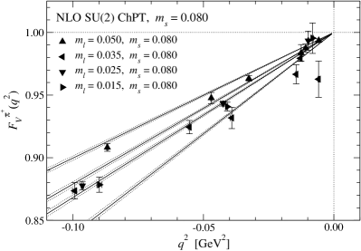
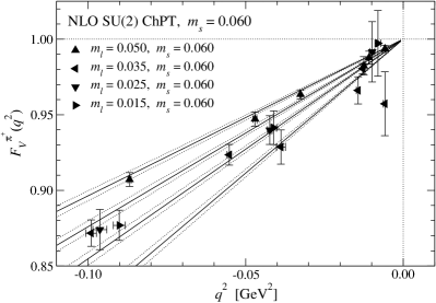
Figure 16: Chiral extrapolation of $F_{V}^{\pi^{+}}$ using NLO SU(2) ChPT formula at $m_{s}\!=\!0.080$ (left panel) and 0.060 (right panel). The data at four different $m_{l}$ are plotted as a function of $t$. Solid and dotted lines show the NLO fit curve and its statistical error. The lines correspond to $m_{l}\!=\!0.050,0.035,0.025$, and 0.015 from top to bottom, respectively.

Figure 16 shows the chiral extrapolation using the NLO expression at each $m_{s}$. The lattice data at the largest and smallest $m_{l}$ tend to deviate from the fit curve and lead to large values of $\chi^{2}/{\rm d.o.f}\!\sim\!1.9$ – 2.9. Note that $l_{6}^{r}$ is the only free parameter appearing at NLO and may be too few to describe both the $m_{l}$ and $t$ dependences. The NNLO fit shown in Fig. 17 describes our data better and $\chi^{2}/{\rm d.o.f}$ is significantly reduced to 0.9 – 1.2.

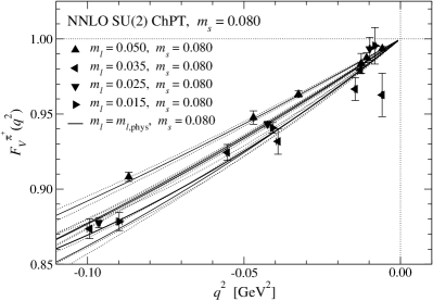
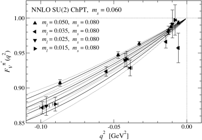
Figure 17: Chiral extrapolation of $F_{V}^{\pi^{+}}$ using NNLO SU(2) ChPT formula. Thin solid lines show the NNLO fit curve at simulated $m_{l}$. In the left panel, we also plot the fit curve at the physical light quark mass $m_{l,\rm phys}$ by the thick solid line. Note that $m_{s}\!=\!0.080$ is close to $m_{s,\rm phys}$.

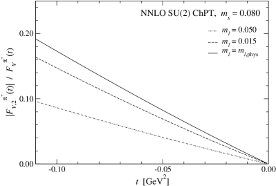
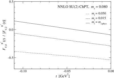
Figure 18: Convergence of chiral expansion at $m_{s}\!=\!0.080$. Left panel: ratio of the NLO contribution to the total $|F_{V,2}^{\pi^{+}}|/F_{V}^{\pi^{+}}$. The dot-dashed, dashed and solid lines show data at $m_{l}\!=\!0.050$, 0.015 and $m_{l,\rm phys}$, respectively. Right panel: ratio of the NLO and NNLO contributions $F_{V,4}^{\pi^{+}}/|F_{V,2}^{\pi^{+}}|$.

The convergence of this NNLO expansion seems reasonable around the physical strange quark mass $m_{s}\!\sim\!m_{s,\rm phys}$ as plotted in Fig. 18. We observe that the NLO contribution $F_{V,2}^{\pi^{+}}$ is at most 20 % of the total value $F_{V}^{\pi^{+}}$ in our simulated region of $t$ and $m_{l}$. The slightly worse convergence at lighter $m_{l}$ is because $F_{V,2}^{\pi^{+}}$ is proportional to $F_{\pi}^{-2}$ in the $\xi$-expansion. The magnitude of the NNLO contribution relative to NLO is about 0.5 at our largest $m_{l}$. It however decreases to $\lesssim 0.1$ – 0.2 around our lightest $m_{l}$ and down to $m_{l,\rm phys}$.

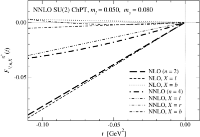
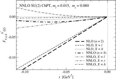
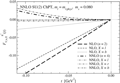
Figure 19: LEC-(in)dependent contributions to $F_{V}^{\pi^{+}}$ in our chiral fit at $m_{s}\!=\!0.080$ based on NNLO SU(2) ChPT. Top left and right panels show data at our simulation points $m_{l}\!=\!0.050$ and 0.015. The bottom panel is at the physical light quark mass $m_{l,\rm phys}$.

For a more detailed look, we decompose the NLO and NNLO contributions into LEC-dependent and independent parts and rewrite the chiral expansion (40) as

$$F_{V}^{\pi^{+}}(t) = F_{V,0}^{\pi^{+}}+F_{V,2,l}^{\pi^{+}}(t)+F_{V,2,b}^{\pi^{+}}(t)+F_{V,4,l}^{\pi^{+}}(t)+F_{V,4,r}^{\pi^{+}}(t)+F_{V,4,b}^{\pi^{+}}(t).$$ (53)

Here $F_{V,2,l}^{\pi^{+}}$ ($F_{V,2,b}^{\pi^{+}}$) represents the $l_{i}^{r}$-dependent (independent) NLO term, which arises from the diagrams shown in Fig. 15 - b (c). The $r_{V,i}^{r}$- and $l_{i}^{r}$- dependent NNLO terms, $F_{V,4,r}^{\pi^{+}}$ and $F_{V,4,l}^{\pi^{+}}$, mainly come from the tree diagrams involving an $\mathcal{L}_{6}$ vertex and the one-loop diagrams with an $\mathcal{L}_{4}$ vertex, respectively. An example of these diagrams is shown in Figs. 15 - d and e. The LEC-independent NNLO term $F_{V,4,b}^{\pi^{+}}$ is from two-loop diagrams such as Fig. 15 - f. Figure 19 compares these terms at $m_{l}\!=\!0.050$, 0.015, and $m_{l,\rm phys}$. We observe that the NLO contribution $F_{V,2}^{\pi^{+}}$ is largely dominated by the $l_{i}^{r}$-dependent analytic term $F_{V,2,l}^{\pi^{+}}$. The NNLO contribution $F_{V,4}^{\pi^{+}}$ is dominated by the $l_{i}^{r}$-dependent term $F_{V,4,l}^{\pi^{+}}$ at our largest $m_{l}$, whereas $r_{V,i}^{r}$-dependent term $F_{V,4,r}^{\pi^{+}}$ tends to dominate $F_{V,4}^{\pi^{+}}$ at smaller $m_{l}$. Therefore the uncertainty due to the use of the phenomenological input for $l_{1,2}^{r}$ and $l_{4}^{r}$ may not be large for our results at physical $m_{l}$, such as the charge radius ${\langle r^{2}\rangle_{V}^{\pi^{+}}}$ (see Eq. (60)). Compared to these LEC-dependent contributions, $F_{V,2,b}^{\pi^{+}}$ and $F_{V,4,b}^{\pi^{+}}$ coming from genuine loop diagrams (namely without $\mathcal{L}_{\{4,6\}}$ vertices) are rather small.

Table 12: Numerical results of chiral fit based on NNLO SU(2) ChPT at $m_{s}\!=\!0.080$ and $0.060$. For the LECs, we quote the values at the renormalization scale $\mu\!=\!M_{\rho}$. The first error is statistical, and the second is systematic one due to the choice of the input $l_{1,2}^{r}$ and $l_{4}^{r}$. We also quote results extrapolated to $m_{s,\rm phys}$.

$m_{s}$	$l_{6}^{r}\!\times\!10^{3}$	$r_{V,1}^{r}\!\times\!10^{5}$	$r_{V,2}^{r}\!\times\!10^{5}$	${\langle r^{2}\rangle_{V}^{\pi^{+}}}$ [fm2]
0.080	-10.65(94)(15)	5.9(5.9)(3.5)	19.9(9.3)(0.1)	0.395(26)(3)
0.060	-10.9(2.4)(0.2)	7(14)(4)	31(19)(0)	0.403(67)$\left({}^{+6}_{-3}\right)$
$m_{s,\rm phys}$	-10.64(94)(15)	5.9(5.9)(3.5)	19.4(9.4)(0.1)	0.395(26)(3)

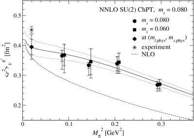
Figure 20: Pion charge radius ${\langle r^{2}\rangle_{V}^{\pi^{+}}}$ as a function of $M_{\pi}^{2}$. The solid line represents ${\langle r^{2}\rangle_{V}^{\pi^{+}}}$ at $m_{s}\!=\!0.080$ reproduced from the NNLO SU(2) ChPT fit. The dashed line shows the NLO contribution. We plot the values in Table 10 by solid circles ($m_{s}\!=\!0.080$) and squares (0.060). The diamond and star are the value extrapolated to the physical point and the experimental value PDG:2014 , respectively.

Numerical results of the NNLO fits at the simulated strange quark masses are summarized in Table 12. We estimate the charge radius ${\langle r^{2}\rangle_{V}^{\pi^{+}}}$ by using these results in the NNLO ChPT expression PFF:ChPT:SU2:NNLO:BCT

$$M_{\pi}^{2}\,{\langle r^{2}\rangle_{V}^{\pi^{+}}} = N\left(-6l_{6}^{r}-L-\frac{1}{N}\right)\xi_{\pi}+N^{2}\left\{-3k_{1,2}-\frac{1}{2}k_{4}+3k_{6}-12l_{4}^{r}l_{6}^{r}\right.$$ (54)

$$\left.+\frac{1}{N}\left(-2l_{4}^{r}+\frac{31}{6}L+\frac{13}{192}+\frac{181}{48N}\right)+6r_{V,1}^{r}\right\}\xi_{\pi}^{2}.$$

As plotted in Fig. 20, the NNLO fit reproduces the values in Table 10, which are evaluated at simulation points assuming $t$-dependence of Eqs. (36) – (38), reasonably well. This figure also shows that the NNLO contribution is significant in our simulation region $M_{\pi}\!\gtrsim\!300$ MeV ($M_{\pi}^{2}\!\gtrsim\!0.09~{}\mbox{GeV}^{2}$ in the horizontal axis of the figure). This is consistent with our previous finding in two-flavor QCD PFF:JLQCD:Nf2:RG+Ovr .

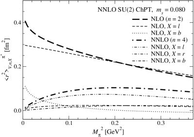
Figure 21: LEC-(in)dependent contributions at NLO and NNLO to ${\langle r^{2}\rangle_{V}^{\pi^{+}}}$.

Similar to the decomposition of $F_{V}^{\pi^{+}}$ in Eq. (53), we express the chiral expansion of ${\langle r^{2}\rangle_{V}^{\pi^{+}}}$ as

$${\langle r^{2}\rangle_{V}^{\pi^{+}}} = {\langle r^{2}\rangle_{V,2}^{\pi^{+}}}+{\langle r^{2}\rangle_{V,4}^{\pi^{+}}},$$ (55)

$${\langle r^{2}\rangle_{V,2}^{\pi^{+}}} = {\langle r^{2}\rangle_{V,2,l}^{\pi^{+}}}+{\langle r^{2}\rangle_{V,2,b}^{\pi^{+}}},\hskip 14.22636pt{\langle r^{2}\rangle_{V,4}^{\pi^{+}}}={\langle r^{2}\rangle_{V,4,l}^{\pi^{+}}}+{\langle r^{2}\rangle_{V,4,r}^{\pi^{+}}}+{\langle r^{2}\rangle_{V,4,b}^{\pi^{+}}}.$$ (56)

Namely, ${\langle r^{2}\rangle_{V,2,l}^{\pi^{+}}}$, ${\langle r^{2}\rangle_{V,4,l}^{\pi^{+}}}$ and ${\langle r^{2}\rangle_{V,4,r}^{\pi^{+}}}$ depend on $l_{i}^{r}$ and $r_{V,i}^{r}$, whereas ${\langle r^{2}\rangle_{V,2,b}^{\pi^{+}}}$ and ${\langle r^{2}\rangle_{V,4,b}^{\pi^{+}}}$ are independent of the LECs. These contributions are plotted as a function of $M_{\pi}^{2}$ in Fig. 21. The NLO contribution is largely dominated by the analytic term ${\langle r^{2}\rangle_{V,2,l}^{\pi^{+}}}$, as $F_{V,2,l}^{\pi^{+}}$ dominates $F_{V,2}^{\pi^{+}}$. The charge radius has been considered as a good quantity to observe the one-loop chiral logarithm $\frac{1}{NF_{(\pi)}^{2}}\ln[M_{\pi}^{2}/\mu^{2}]$, which is not suppressed by a multiplicative factor $M_{\pi}^{2}$ and hence diverges toward the chiral limit. In our notation, this is included in the NLO loop correction ${\langle r^{2}\rangle_{V,2,b}^{\pi^{+}}}$ but becomes significant only at $M_{\pi}\!\lesssim\!300$ MeV, namely below our simulation points. In addition, the enhancement of ${\langle r^{2}\rangle_{V,2,b}^{\pi^{+}}}$ is partly compensated by the decrease of the NNLO contribution, particularly of ${\langle r^{2}\rangle_{V,4,l}^{\pi^{+}}}$. Therefore, we may be able to clearly observe the logarithmic singularity only near the chiral limit. Our work in the so-called $\epsilon$-regime PFF:JLQCD:Nf3:RG+Ovr:e-regime is an interesting step in this direction.

The NNLO contribution ${\langle r^{2}\rangle_{V,4}^{\pi^{+}}}$ turns out to be a 30 – 50% correction at the simulated values of $M_{\pi}^{2}$ and becomes small, $\lesssim\!10$ %, only near the physical point. The two-loop term ${\langle r^{2}\rangle_{V,4,b}^{\pi^{+}}}$ is rather small. The analytic term ${\langle r^{2}\rangle_{V,4,r}^{\pi^{+}}}$ vanishes towards the chiral limit, whereas the similar term $F_{V,4,r}^{\pi^{+}}$ is not a small correction to $F_{V}^{\pi^{+}}$. This is because $O(t^{2})$ term of $F_{V}^{\pi^{+}}$ with $r_{V,2}^{r}$ does not contribute to ${\langle r^{2}\rangle_{V}^{\pi^{+}}}$, and ${\langle r^{2}\rangle_{V,4,r}^{\pi^{+}}}\!=\!6Nr_{V,1}^{r}\xi_{\pi}/F_{\pi}^{2}$ is suppressed by $M_{\pi}^{2}$ in the chiral limit. Hence the $l_{i}^{r}$-dependent term ${\langle r^{2}\rangle_{V,4,l}^{\pi^{+}}}$ gives the largest contribution at NNLO. Note that this term has non-trivial $M_{\pi}^{2}$ dependence: roughly constant down to $M_{\pi}\!\simeq\!400$ MeV and non-linearly decreases towards the chiral limit. It is therefore important to correctly take account of the NNLO contributions for a reliable chiral extrapolation of ${\langle r^{2}\rangle_{V}^{\pi^{+}}}$.

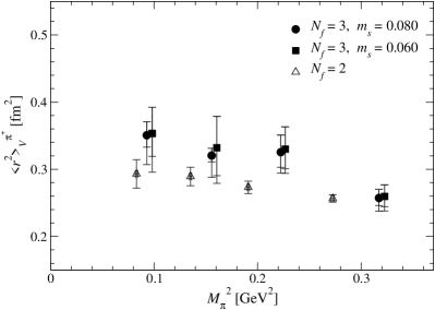
Figure 22: Comparison of ${\langle r^{2}\rangle_{V}^{\pi^{+}}}$ between three-flavor QCD (solid circles and squares) and two-flavor QCD (open triangles) PFF:JLQCD:Nf2:RG+Ovr . The latter was obtained on $16^{3}\times 32$ at $a=0.118(2)$ fm with four times higher statistics, but $|t|\!\gtrsim\!(\mbox{500 MeV})^{2}$ without the twisted boundary conditions. For a fair comparison, we use the lattice spacing determined from $r_{0}\!=\!0.49$ fm r0 to convert all data to physical units.

In SU(2) ChPT, the $m_{s}$ dependence of physical quantities is encoded in that of LECs. We need to extrapolate our results to the physical strange quark mass $m_{s,\rm phys}$ in order to obtain information about the real world. As far as the pion observables $F_{V}^{\pi^{+}}$ and ${\langle r^{2}\rangle_{V}^{\pi^{+}}}$ are concerned, the $m_{s}$ dependence turns out to be mild as suggested by the good stability of ${\langle r^{2}\rangle_{V}^{\pi^{+}}}$ between $m_{s}\!=\!0.080$ and 0.060 as shown in Fig. 20. This is confirmed also in Fig. 22, which shows that the difference in ${\langle r^{2}\rangle_{V}^{\pi^{+}}}$ between three- and two-flavor QCD is not large.

For the extrapolation of $l_{6}^{r}$ and ${\langle r^{2}\rangle_{V}^{\pi^{+}}}$, we parametrize their $m_{s}$ dependence by a linear function including the NLO chiral logarithm ChPT:SU3:NLO

$$l_{6}^{r} = a_{l,0}+\frac{1}{12N}\ln\left[M_{K}^{2}\right]+a_{l,1}\,m_{s},$$ (57)

$${\langle r^{2}\rangle_{V}^{\pi^{+}}} = a_{r^{2},0}-\frac{1}{2NF_{\pi}^{2}}\ln\left[M_{K}^{2}\right]+a_{r^{2},1}\,m_{s}.$$ (58)

Figure 23 shows that the logarithmic term $\ln[M_{K}^{2}]$ becomes significant only near the $m_{s}\!=\!0$ limit, and that the simulated value $m_{s}\!=\!0.080$ is close to $m_{s,\rm phys}$. Moreover, the $m_{s}$ dependence is rather mild as discussed above. The extrapolation therefore does not deteriorate the statistical accuracy, and is stable against the choice of the parametrization form: for instance, removing the logarithmic term and/or including an $O(m_{s}^{2})$ correction. These observations lead us to employ a simple linear form

$$r_{V,i}^{r} = a_{r_{i},0}+a_{r_{i},1}m_{s}$$ (59)

for $r_{V,i}^{r}$, which has the large statistical error.

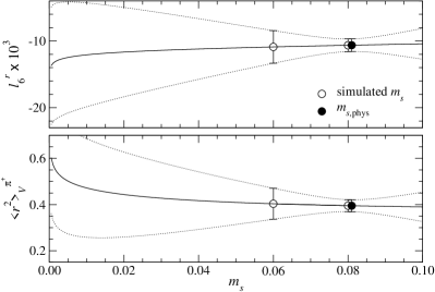
Figure 23: Extrapolation of $l_{6}^{r}$ (top panel) and ${\langle r^{2}\rangle_{V}^{\pi^{+}}}$ (bottom panel) to $m_{s,\rm phys}$.

The extrapolated values are summarized in Table 12. We obtain

$${\langle r^{2}\rangle_{V}^{\pi^{+}}} = 0.395(26)(3)(32)~{}\mbox{fm}^{2},$$ (60)

where the first error is statistical, and the second one is the systematic error due to the choice of the input values of $l_{i}^{r}$. The third is the discretization error at our finite lattice spacing, which is conservatively estimated by an order counting $O((a\Lambda_{\rm QCD})^{2})\!\sim\!8$ % with $\Lambda_{\rm QCD}\!=\!500$ MeV. Our result of ${\langle r^{2}\rangle_{V}^{\pi^{+}}}$ is consistent with the experimental value ${\langle r^{2}\rangle_{V}^{\pi^{+}}}\!=\!0.452(11)~{}\mbox{fm}^{2}$ PDG:2014 within estimated uncertainties. Note that the systematic error due to the choice of the inputs $l_{1,2}^{r}$ and $l_{4}^{r}$ is rather small for this quantity, because only the NNLO $l_{i}^{r}$-dependent terms, $F_{V,4,l}^{\pi^{+}}$ and ${\langle r^{2}\rangle_{V,4,l}^{\pi^{+}}}$, contain these inputs and decrease towards the physical point.

For the $O(p^{4})$ coupling, we obtain

$$\bar{l}_{6} = 13.49(89)(14)(81)\hskip 14.22636pt(l_{6}^{r}=-10.64(94)(15)(86)\!\times\!10^{-3}).$$ (61)

This is consistent with our estimate $\bar{l}_{6}\!=\!11.9(1.2)$ in two-flavor QCD PFF:JLQCD:Nf2:RG+Ovr as well as with phenomenological estimates $16.0(0.9)$ PFF:ChPT:SU2:NNLO:BCT from the experimental data of $F_{V}^{\pi^{+}}$, and 15.2(4) obtained together with the $\pi\!\to\!e\nu\gamma$ decay and the $V\!-\!A$ spectral function ChPT:l6:GPP ; ChPT:LECs:SU2+SU3 . Our results for the $O(p^{6})$ couplings at $\mu\!=\!M_{\rho}$ are

$$r_{V,1}^{r} = 5.9(5.9)(3.5)(0.5)\times 10^{-5},$$ (62)

$$r_{V,2}^{r} = 19.4(9.4)(0.1)(1.6)\times 10^{-5}.$$ (63)

V Chiral extrapolation based on SU(3) ChPT

In this section, we extend our analysis to SU(3) ChPT, which is applicable also to the kaon EM form factors $F_{V}^{K^{+}}$ and $F_{V}^{K^{0}}$. According to Ref. PFF+KFF:ChPT:NNLO:Nf3 and similar to Eq. (53), we write the chiral expansion of the EM form factors of the light mesons ($P\!=\!\pi^{+},K^{+},K^{0}$) as

$$F_{V}^{P}(t) = F_{V,0}^{P}+F_{V,2}^{P}(t)+F_{V,4}^{P}(t)+F_{V,6}^{P}(t),$$ (64)

$$F_{V,2}^{P}(t) = F_{V,2,L}^{P}(t)+F_{V,2,B}^{P}(t),\hskip 14.22636ptF_{V,4}^{P}(t)=F_{V,4,L}^{P}(t)+F_{V,4,C}^{P}(t)+F_{V,4,B}^{P}(t).$$ (65)

Here $F_{V,0}^{P}$, $F_{V,2,B}^{P}$ and $F_{V,4,B}^{P}$ are LEC-independent LO, NLO and NNLO contributions, whereas $F_{V,2,L}^{P}$, $F_{V,4,L}^{P}$ and $F_{V,4,C}^{P}$ depend on the LECs. Because $m_{s}\!\gg\!m_{l}$, the chiral expansion in SU(3) ChPT may have poorer convergence than in SU(2) ChPT. Hence we include a possible higher order correction $F_{V,6}^{P}$, the explicit form of which is not known in ChPT. The vector current conservation states that the LO contribution for the charged mesons is

$$F_{V,0}^{\pi^{+}}=F_{V,0}^{K^{+}}=1.$$ (66)

The NLO analytic term

$$F_{V,2,L}^{\pi^{+}}(t)=F_{V,2,L}^{K^{+}}(t)=\frac{2}{F_{\pi}^{2}}L_{9}^{r}t$$ (67)

arises from the diagram Fig. 15 - b with a vertex from $\mathcal{L}_{4}$, which involves the $O(p^{4})$ coupling $L_{9}^{r}$. In contrast, these contributions vanish,

$$F_{V,0}^{K^{0}}=F_{V,2,L}^{K^{0}}(t)=0,$$ (68)

for the neutral kaon EM form factor, which is the difference of the light and strange quark currents as written in Eq. (32).

The term $F_{V,2,B}^{P}$ represents the LEC-independent NLO contribution coming from one-loop diagrams, such as Fig. 15 - c, and is given by

$$F_{\pi}^{2}\,F_{V,2,B}^{\pi^{+}}(t) = {\bar{A}(M_{\pi}^{2})}+\frac{1}{2}{\bar{A}(M_{K}^{2})}-2{\bar{B}_{22}(M_{\pi}^{2},M_{\pi}^{2},t)}-{\bar{B}_{22}(M_{K}^{2},M_{K}^{2},t)},$$ (69)

$$F_{\pi}^{2}\,F_{V,2,B}^{K^{+}}(t) = \frac{1}{2}{\bar{A}(M_{\pi}^{2})}+{\bar{A}(M_{K}^{2})}-{\bar{B}_{22}(M_{\pi}^{2},M_{\pi}^{2},t)}-2{\bar{B}_{22}(M_{K}^{2},M_{K}^{2},t)},$$ (70)

$$F_{\pi}^{2}\,F_{V,2,B}^{K^{0}}(t) = -\frac{1}{2}{\bar{A}(M_{\pi}^{2})}+\frac{1}{2}{\bar{A}(M_{K}^{2})}+{\bar{B}_{22}(M_{\pi}^{2},M_{\pi}^{2},t)}-{\bar{B}_{22}(M_{K}^{2},M_{K}^{2},t)},$$ (71)

where $\bar{A}$ ($\bar{B}_{22}$) represents $t$-independent (dependent) one-loop integral function. Their definition and expression are summarized in Appendix A.

The LEC-independent NNLO term $F_{V,4,B}^{P}$ involves two-loop integrals, and hence its expression is rather complicated. See Appendix B for more details. We note, however, that this term in the $\xi$-expansion does not contain any free parameter, and is not an obstacle to obtaining a stable chiral extrapolation.

The $L_{i}^{r}$-dependent NNLO term $F_{V,4,L}^{P}$ mainly comes from one-loop diagrams with one vertex from $\mathcal{L}_{4}$, such as Fig. 15 - e . This term can be expressed with $L_{i}^{r}$ and the one-loop integral functions as

$$F_{\pi}^{4}\,F_{V,4,L}^{\pi^{+}}(t) = 8M_{\pi}^{2}\,(2L_{4}^{r}+L_{5}^{r}){\bar{A}(M_{\pi}^{2})}+4M_{\pi}^{2}L_{5}^{r}{\bar{A}(M_{K}^{2})}+tL_{9}^{r}\,\left\{6{\bar{A}(M_{\pi}^{2})}+3{\bar{A}(M_{K}^{2})}\right\}$$ (72)

$$+\left\{-16(2L_{4}^{r}+L_{5}^{r})M_{\pi}^{2}+4(4L_{1}^{r}-2L_{2}^{r}+2L_{3}^{r}-L_{9}^{r})t\right\}{\bar{B}_{22}(M_{\pi}^{2},M_{\pi}^{2},t)}$$

$$+(-8L_{5}^{r}M_{\pi}^{2}+4L_{3}^{r}t-2L_{9}^{r}t){\bar{B}_{22}(M_{K}^{2},M_{K}^{2},t)},$$

$$F_{\pi}^{4}\,F_{V,4,L}^{K^{+}}(t) = (16L_{4}^{r}M_{K}^{2}+8L_{5}^{r}M_{\pi}^{2}){\bar{A}(M_{K}^{2})}+4L_{5}^{r}M_{\pi}^{2}{\bar{A}(M_{\pi}^{2})}+L_{9}^{r}t\,\left\{5{\bar{A}(M_{\pi}^{2})}+4{\bar{A}(M_{K}^{2})}\right\}$$ (73)

$$+\left\{-32L_{4}^{r}M_{K}^{2}-16L_{5}^{r}M_{\pi}^{2}+4(4L_{1}^{r}-2L_{2}^{r}+2L_{3}^{r}-L_{9}^{r})t\right\}{\bar{B}_{22}(M_{K}^{2},M_{K}^{2},t)}$$

$$+(-8L_{5}^{r}M_{\pi}^{2}+4L_{3}^{r}t-2L_{9}^{r}t){\bar{B}_{22}(M_{\pi}^{2},M_{\pi}^{2},t)}+16L_{5}^{r}L_{9}^{r}(M_{\pi}^{2}-M_{K}^{2})t,$$

$$F_{\pi}^{4}\,F_{V,4,L}^{K^{0}}(t) = (4L_{5}^{r}M_{\pi}^{2}+L_{9}^{r}t)\left\{-{\bar{A}(M_{\pi}^{2})}+{\bar{A}(M_{K}^{2})}\right\}$$ (74)

$$+\left\{8L_{5}^{r}M_{\pi}^{2}-2(2L_{3}^{r}-L_{9}^{r})t\right\}\left\{{\bar{B}_{22}(M_{\pi}^{2},M_{\pi}^{2},t)}-{\bar{B}_{22}(M_{K}^{2},M_{K}^{2},t)}\right\}.$$

Table 13: Input values for $O(p^{4})$ couplings in SU(3) ChPT taken from Ref. ChPT:LECs:SU2+SU3 . The central value and first error are from the authors’ preferred fit “BE14”, whereas we assign the difference from the other fit (see text) as the second error.

$L_{1}^{r}\!\times\!10^{3}$	$L_{2}^{r}\!\times\!10^{3}$	$L_{3}^{r}\!\times\!10^{3}$	$L_{4}^{r}\!\times\!10^{3}$	$L_{5}^{r}\!\times\!10^{3}$
0.53(6)(+11)	0.81(4)(-22)	-3.07(20)(+27)	0.3(0)(+0.46)	1.01(6)(-51)

Together with Eq. (67), we have the single $O(p^{4})$ coupling $L_{9}^{r}$ at NLO, and additional five $L_{\{1\,-\,5\}}$ at NNLO. Similar to our analysis in SU(2) ChPT, we treat $L_{9}^{r}$ as a fitting parameter, and fix others to a phenomenological estimate. In Ref. ChPT:LECs:SU2+SU3 , the authors present two types of the NNLO ChPT fit of experimental data, such as the meson masses and decay constants. A fit called “BE14” fixes $L_{4}^{r}$ to a fiducial value $0.3\!\times\!10^{-3}$, since this is difficult to determine due to the strong (anti-)correlation with $F_{0}$. (We note that the renormalization scale is set to $\mu\!=\!M_{\rho}$ also in this section.) The other fit without the constraint on $L_{4}^{r}$ obtains $L_{4}^{r}\!=\!0.76(18)\!\times\!10^{-3}$, which is slightly higher than that for BE14. In our analysis, we employ the authors’ preferred fit BE14 and consider the difference between BE14 and the free-fit as an additional uncertainty of $L_{i}^{r}$. These input values are summarized in Table 13.

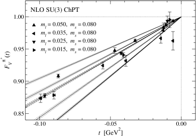
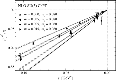
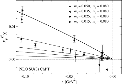
Figure 24: Chiral extrapolations of $F_{V}^{\pi^{+}}$ (top left panel), $F_{V}^{K^{+}}$ (top right panel) and $F_{V}^{K^{0}}$ (bottom panel) based on NLO SU(3) ChPT. Triangles and thin lines show our data and their fit curves at $m_{s}\!=\!0.080$. We also plot the fit curve at the physical point $(m_{l,\rm phys},m_{s,\rm phys})$ by the thick lines. Note that there is no tunable parameter for $F_{V}^{K^{0}}$ at NLO.

The most important issue to obtain a stable chiral extrapolation is how to deal with $O(p^{6})$ couplings $C_{i}^{r}$ ChPT:SU3:NNLO in the NNLO analytic term $F_{V,4,C}^{P}$, since these couplings are in general poorly known in phenomenology. The three NNLO analytic terms have six independent parameter dependences

$$F_{\pi}^{4}\,F_{V,4,C}^{\pi^{+}}(t) = -4{c_{\pi^{+},\pi t}^{r}}\,M_{\pi}^{2}\,t-8{c_{\pi^{+},Kt}^{r}}\,M_{K}^{2}\,t-4{c_{t^{2}}^{r}}\,t^{2},$$ (75)

$$F_{\pi}^{4}\,F_{V,4,C}^{K^{+}}(t) = -4{c_{K^{+},\pi t}^{r}}\,M_{\pi}^{2}\,t-4c_{K^{+},Kt}^{r}\,M_{K}^{2}\,t-4{c_{t^{2}}^{r}}\,t^{2},$$ (76)

$$F_{\pi}^{4}\,F_{V,4,C}^{K^{0}}(t) = -\frac{8}{3}\,{c_{K^{0}}^{r}}\,(M_{K}^{2}-M_{\pi}^{2})\,t,$$ (77)

and seven $C_{i}^{r}$’s enter into these six coefficients through the $\mathcal{L}_{6}$ vertex in Fig. 15 - d

$${c_{\pi^{+},\pi t}^{r}} = 4C_{12}^{r}+4C_{13}^{r}+2C_{63}^{r}+C_{64}^{r}+C_{65}^{r}+2C_{90}^{r},$$ (78)

$${c_{\pi^{+},Kt}^{r}} = 4C_{13}^{r}+C_{64}^{r},$$ (79)

$${c_{t^{2}}^{r}} = C_{88}^{r}-C_{90}^{r},$$ (80)

$${c_{K^{+},\pi t}^{r}} = 4C_{13}^{r}+\frac{2}{3}C_{63}^{r}+C_{64}^{r}-\frac{1}{3}C_{65}^{r},$$ (81)

$$c_{K^{+},Kt}^{r} = 4C_{12}^{r}+8C_{13}^{r}+\frac{4}{3}C_{63}^{r}+2C_{64}^{r}+\frac{4}{3}C_{65}^{r}+2C_{90}^{r},$$ (82)

$${c_{K^{0}}^{r}} = 2C_{63}^{r}-C_{65}^{r}.$$ (83)

Hence our chiral fit can not determine all these $O(p^{6})$ couplings separately, but the six coefficients. We note that these are not totally independent:

$${c_{K^{+},\pi t}^{r}} = {c_{\pi^{+},Kt}^{r}}+\frac{1}{3}{c_{K^{0}}^{r}},$$ (84)

$$c_{K^{+},Kt}^{r} = {c_{\pi^{+},\pi t}^{r}}+{c_{\pi^{+},Kt}^{r}}-\frac{1}{3}{c_{K^{0}}^{r}}.$$ (85)

We carry out simultaneous fit to $F_{V}^{\pi^{+}}$, $F_{V}^{K^{+}}$ and $F_{V}^{K^{0}}$, in which four coefficients ${c_{\pi^{+},\pi t}^{r}}$, ${c_{\pi^{+},Kt}^{r}}$, ${c_{t^{2}}^{r}}$ and ${c_{K^{0}}^{r}}$ are treated as fitting parameters.

Our chiral fit based on NLO SU(3) ChPT is plotted in Fig. 24. Similar to the analysis in SU(2) ChPT, the NLO formula is poorly fitted to our data resulting in a rather large value of $\chi^{2}/{\rm d.o.f}\sim 8.3$. Note that SU(3) chiral symmetry constrains the dependence of the form factors on $m_{l}$, $m_{s}$ and $t$, and allows only single tunable parameter at NLO; namely $L_{9}^{r}$ to describe $t$ dependence of $F_{V}^{\pi^{+}}$ and $F_{V}^{K^{+}}$. Consequently, the NLO formula fails to reproduce the $m_{l}$ dependence particularly of $F_{V}^{K^{0}}$.

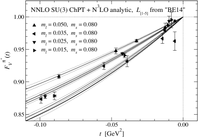
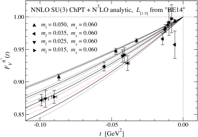
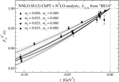
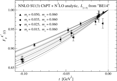
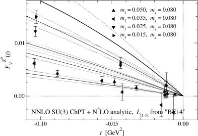
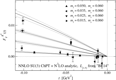
Figure 25: Chiral extrapolations of $F_{V}^{\pi^{+}}$ (top panels), $F_{V}^{K^{+}}$ (middle panels) and $F_{V}^{K^{0}}$ (bottom panels) based on NNLO SU(3) ChPT. The left and right panels show our data at $m_{s}\!=\!0.080$ and 0.060. In the left panel for $m_{s}\!=\!0.080\!\sim\!m_{s,\rm phys}$, we also plot the fit curve at the physical point $(m_{l,\rm phys},m_{s,\rm phys})$ by the thick lines.

The value of $\chi^{2}/{\rm d.o.f}$ is largely decreased to 2.3 by taking account of the NNLO contribution. We observe that simulation data of $F_{V}^{K^{0}}$ tend to deviate from the NNLO fit curve and give rise to a large part of $\chi^{2}$. Since $F_{V}^{K^{0}}$ has only single free parameter ${c_{K^{0}}^{r}}$ even at NNLO, we also test a fitting form with an N³LO analytic correction

$$F_{V,6}^{\pi^{+}}=F_{V,6}^{K^{+}}=0,\hskip 14.22636ptF_{V,6}^{K^{0}}=\frac{{d_{K^{0}}}}{F_{\pi}^{6}}\,M_{\pi}^{2}\,(M_{K}^{2}-M_{\pi}^{2})\,t.$$ (86)

Note that the factor $(M_{K}^{2}-M_{\pi}^{2})\,t$ in $F_{V,6}^{K^{0}}$ is needed to satisfy $F_{V}^{K^{0}}(0)\!=\!0$ (vector current conservation) and $F_{V}^{K^{0}}(t)\!=\!0$ in the SU(3) symmetric limit (see, Eq. (32)). This fit is plotted in Fig. 25 and leads to a slightly smaller $\chi^{2}/{\rm d.o.f.}\!=\!1.8$. Including more terms at N³LO and even higher orders reduces $\chi^{2}$ only slightly, and the fitting parameters in these corrections are poorly determined. We therefore employ the NNLO ChPT fit including the N³LO correction (86) in the following discussion.

Numerical results of the fit are summarized in Table 14. We estimate the systematic error due to the choice of the input $L_{\{1,\cdots,5\}}$ by shifting each of $L_{\{1,\cdots,5\}}$ by its uncertainty quoted in Table 13. In our analysis, the choice of $L_{3}$ and $L_{5}$ tends to lead to the largest deviation in the fitting results. This systematic uncertainty from $L_{\{1,\cdots,5\}}$ is generally well below the statistical error, because the $L_{i}^{r}$-dependent term $F_{V,4,L}^{\{\pi^{+},K^{+}\}}$ is not a dominant contribution at NNLO (see below).

Table 14: Numerical results of chiral fit based on NNLO SU(3) ChPT. LECs are the values at the renormalization scale $\mu\!=\!M_{\rho}$. The first error is statistical, and the second is systematic one due to the choice of the input $L_{\{1,\cdots,5\}}^{r}$. We also quote ${c_{K^{+},\pi t}^{r}}$ and $c_{K^{+},Kt}^{r}$ calculated using Eqs. (84) – (85).

$L_{9}^{r}\!\times\!10^{3}$	${c_{\pi^{+},\pi t}^{r}}\!\times\!10^{5}$	${c_{\pi^{+},Kt}^{r}}\!\times\!10^{5}$	${c_{t^{2}}^{r}}\!\times\!10^{5}$
$4.6(1.1)\left({}^{+0.1}_{-0.5}\right)$	$-1.95(84)\left({}^{+38}_{-21}\right)$	$-1.4(1.2)\left({}^{+0.1}_{-0.7}\right)$	$-6.4(1.1)(0.1)$
${c_{K^{0}}^{r}}\!\times\!10^{5}$	${d_{K^{0}}}\!\times\!10^{7}$	${c_{K^{+},\pi t}^{r}}\!\times\!10^{5}$	$c_{K^{+},Kt}^{r}\!\times\!10^{5}$
$0.15(62)\left({}^{+12}_{-7}\right)$	$-37(12)(2)$	$-1.3(1.2)\left({}^{+0.1}_{-0.7}\right)$	$-3.4(1.9)\left({}^{+0.1}_{-0.3}\right)$

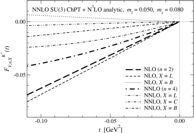
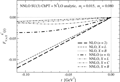
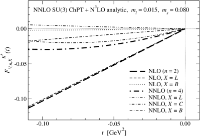
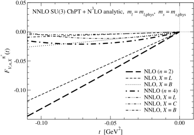
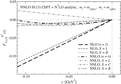
Figure 26: LEC-(in)dependent NLO and NNLO contributions in our chiral fit based on NNLO SU(3) ChPT. The left and right panels show data for $F_{V}^{\pi^{+}}$ and $F_{V}^{K^{+}}$, whereas top, middle and bottom panels are for $(m_{l},m_{s})\!=\!(0.050,0.080)$, (0.015,0.080) and the physical point $(m_{l,\rm phys},m_{s,\rm phys})$, respectively.

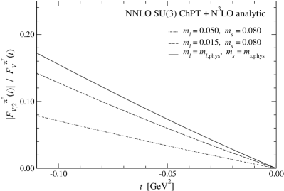
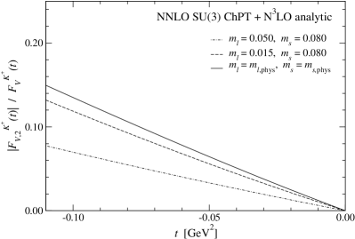
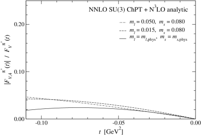
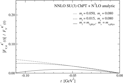
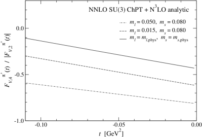
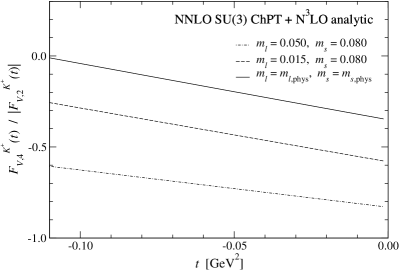
Figure 27: Convergence of chiral expansion of $F_{V}^{\pi^{+}}$ (left panels) and $F_{V}^{K^{+}}$ (right panels) near $m_{s,\rm phys}$. Top panels: ratio of the NLO contribution to the total $|F_{V,2}^{\{\pi^{+},K^{+}\}}|/F_{V}^{\{\pi^{+},K^{+}\}}$. The dot-dashed (dashed) line shows data at $m_{l}\!=\!0.050$ (0.015) and $m_{s}\!=\!0.080$, whereas the solid line is at $(m_{l,\rm phys},m_{s,\rm phys})$. Middle panels: ratio of the NNLO contribution to the total $|F_{V,4}^{\{\pi^{+},K^{+}\}}|/F_{V}^{\{\pi^{+},K^{+}\}}$. Bottom panels: ratio of the NNLO and NLO contributions $F_{V,4}^{\{\pi^{+},K^{+}\}}/|F_{V,2}^{\{\pi^{+},K^{+}\}}|$.

In Figures 26 and 27, we examine the convergence of the chiral expansion of $F_{V}^{\pi^{+}}$, which is now explicitly depends on $m_{s}$ in SU(3) ChPT. Figure 26 shows a decomposition to the LEC-dependent and independent terms in Eqs. (64) – (65). Similar to our SU(2) ChPT fit, the NLO contribution $F_{V,2}^{\pi^{+}}$ is largely dominated by the analytic term $F_{V,2,L}^{\pi^{+}}$ with $L_{9}^{r}$. The loop term $F_{V,2,B}^{\pi^{+}}$ is a small correction compared to $F_{V,2,L}^{\pi^{+}}$, but increases towards the physical point possibly due to the enhancement of the chiral logarithms $\propto\!\ln[M_{\pi}^{2}/\mu]$.

This can also be seen in Fig. 27, where we plot ratios $|F_{V,2}^{\pi^{+}}|/F_{V}^{\pi^{+}}$ (NLO/total), $|F_{V,4}^{\pi^{+}}|/F_{V}^{\pi^{+}}$ (NNLO/total), and $F_{V,4}^{\pi^{+}}/|F_{V,2}^{\pi^{+}}|$ (NNLO/NLO). We observe larger $|F_{V,2}^{\pi^{+}}|/F_{V}^{\pi^{+}}$ at smaller $m_{l}$ not only due to the enhancement of $F_{V,2,B}^{\pi^{+}}$ but also because $F_{V,2,L}^{\pi^{+}}$ is enhanced by $F_{\pi}^{-2}$ in the $\xi$-expansion. It turns out that, however, $F_{V,2}^{\pi^{+}}$ is reasonably small correction at most $\sim\!15$ % at $m_{l}\!=\!m_{l,\rm phys}$ and $t\!\sim\!-(300~{}\mbox{MeV})^{2}$. It decreases towards smaller $t$ because of the vector current conservation $F_{V}^{\pi^{+}}(0)\!=\!F_{V,0}^{\pi^{+}}\!=1$.

We observe in Fig. 27 that the NNLO contribution is even smaller in the whole region of $M_{\pi}^{2}$, $M_{K}^{2}$ and $t$. Figure 26 shows that the analytic term $F_{V,4,C}^{\pi^{+}}$ is the largest NNLO contribution at the largest $m_{l}$. The first two terms in Eqs. (75) – (76) largely contribute to $F_{V,4,C}^{\{\pi^{+},K^{+}\}}$, because we simulate $|t|\!\lesssim\!M_{\pi}^{2},M_{K}^{2}$, and the coefficients ${c_{\pi^{+},\pi t}^{r}}$, ${c_{\pi^{+},Kt}^{r}}$ and ${c_{t^{2}}^{r}}$ are of the same order. Towards the chiral limit, these terms are suppressed by the NG boson masses, $M_{\pi}^{2}$ and $M_{K}^{2}$, and hence $F_{V,4}^{\pi^{+}}$ decreases, whereas $F_{V,2}^{\pi^{+}}$ increases in this limit. This is why the magnitude of $F_{V,4}^{\pi^{+}}/|F_{V,2}^{\pi^{+}}|$ rapidly decreases at smaller $m_{l}$ as shown in the bottom panels of Fig. 27. Namely, the convergence between NNLO and NLO is largely improved towards the chiral limit.

While $F_{V,4}^{\pi^{+}}/|F_{V,2}^{\pi^{+}}|$ $\gtrsim\!0.5$ at the largest $m_{l}$, we do not expect large N³LO nor even higher order corrections. We note that, around our largest $|t|\!\sim\!(300~{}\mbox{MeV})^{2}$, the NNLO correction $F_{V,4}^{\pi^{+}}$ is statistically insignificant: namely, it has $\gtrsim\!50$ % statistical error. Towards $t\!=\!0$, the error decreases but its central value also decreases due to the vector current conservation: at $|t|\!\lesssim\!(150~{}\mbox{MeV})^{2}$, for instance, $F_{V,4}^{\pi^{+}}$ is sub-% correction with the statistical accuracy of $\gtrsim\!30$ %. We therefore expect that even smaller N³LO correction is insignificant within our accuracy, and conclude that our data of $F_{V}^{\pi^{+}}$ are reasonably well described by NNLO SU(3) ChPT.

A comparison with Figs. 18 and 19 suggests that the convergence of the chiral expansion of $F_{V}^{\pi^{+}}$ is not quite different between SU(2) and SU(3) ChPT.

The right panels of Figs. 26 and 27 suggest similar convergence properties for $F_{V}^{K^{+}}$, which involves the strange quarks as the valence degree of freedom in contrast to $F_{V}^{\pi^{+}}$. This is mainly because the NLO contribution $F_{V,2}^{K^{+}}$ is dominated by the analytic term $F_{V,2,L}^{K^{+}}$, which mildly depends on $m_{l}$ and $m_{s}$ only through the factor $F_{\pi}^{-2}$. At NNLO, in addition, a large part of $F_{V,4}^{K^{+}}$ is composed of the analytic term $F_{V,4,C}^{K^{+}}$, and the coefficients in Eqs. (75) – (76) for $F_{V}^{\pi^{+}}$ and $F_{V}^{K^{+}}$ are of the same magnitude: namely ${c_{\pi^{+},\pi t}^{r}}\!\approx\!{c_{K^{+},\pi t}^{r}}$ and ${c_{\pi^{+},Kt}^{r}}\!\approx\!c_{K^{+},Kt}^{r}$.

Interestingly, we observe that the charged meson vector form factors, $F_{V}^{\pi^{+}}$ and $F_{V}^{K^{+}}$, are dominated by the NLO analytic term. A comparison between the analytic and loop terms in ChPT formulae leads to a naive order estimate $L_{i}^{r}\!=\!O((4\pi)^{-2})\!=\!O(6\!\times\!10^{-3})$ and $C_{i}^{r}\!=\!O((4\pi)^{-4})\!=\!O(4\!\times\!10^{-5})$ ChPT:LECs:SU2+SU3 . Our fit results are roughly consistent with this order estimate suggesting that the magnitude of the analytic terms $F_{V,2,L}^{\{\pi^{+},K^{+}\}}$ and $F_{V,4,C}^{\{\pi^{+},K^{+}\}}$ is not unexpectedly large, but loop terms are small. We in fact observe a large cancellation among the two-loop diagrams with the reducible, sunset and vertex integrals (see Appendix B, for their definition) possibly to satisfy $F_{V,4,B}^{\{\pi^{+},K^{+}\}}(0)\!=\!0$ required from the vector current conservation.

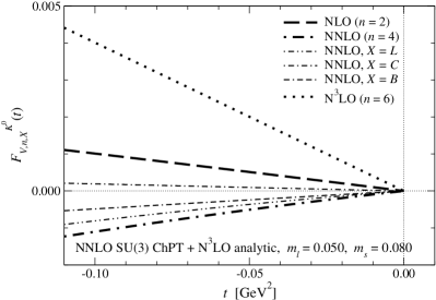
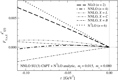
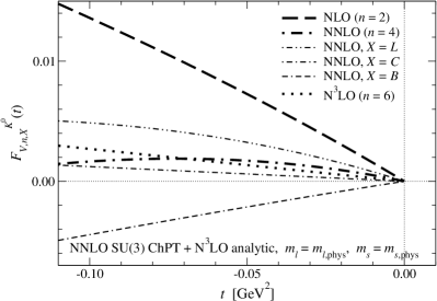
Figure 28: Same as Fig. 26, but for $F_{V}^{K^{0}}$.

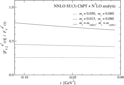
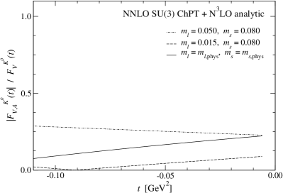
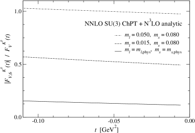
Figure 29: Convergence of chiral expansion of $F_{V}^{K^{0}}$. Top left, top right and bottom panels show $|F_{V,2}^{K^{0}}|/F_{V}^{K^{0}}$, $|F_{V,4}^{K^{0}}|/F_{V}^{K^{0}}$ and $|F_{V,6}^{K^{0}}|/F_{V}^{K^{0}}$, respectively. The dot-dashed (dashed) line shows data at $m_{l}\!=\!0.050$ (0.015) and $m_{s}\!=\!0.080$, whereas the solid line is at $(m_{l,\rm phys},m_{s,\rm phys})$. Note that $F_{V,0}^{K^{0}}\!=\!0$ and the chiral expansion starts from $F_{V,2}^{K^{0}}$.

The neutral kaon form factor $F_{V}^{K^{0}}$ is the difference between the light and strange quark current contributions as seen in Eq. (32). While the LO and NLO analytic terms dominate $F_{V}^{\{\pi^{+},K^{+}\}}$, these for $F_{V}^{K^{0}}$, namely $F_{V,0}^{K^{0}}$ and $F_{V,2,L}^{K^{0}}$, vanish even at $t\!\neq\!0$. As a result, $F_{V}^{K^{0}}$ shows much poorer convergence than $F_{V}^{\{\pi^{+},K^{+}\}}$ as examined in Figs. 28 and 29. There is only the parameter-free term $F_{V,2,B}^{K^{0}}$ within NLO. At the largest $m_{l}$, this term is rather small compared to our simulation results, and hence the large part of $F_{V}^{K^{0}}$ is composed of higher order corrections $F_{V,4}^{K^{0}}+F_{V,6}^{K^{0}}$. However, $F_{V,2,B}^{K^{0}}$ increases as we approach to $m_{l,\rm phys}$ with $m_{s}$ held fixed. This is in accordance with the VMD hypothesis (35): larger $F_{V}^{K^{0}}$ with larger $M_{\phi}-M_{\rho}$. As a result, the convergence is rapidly improved towards the physical point, where both NNLO and N³LO corrections become small compared to the leading term $F_{V,2}^{K^{0}}$.

We also note that the large N³LO contributions $F_{V,6}^{K^{0}}$ may be partly attributed to the fact that the analytic NNLO and N³LO contributions, $F_{V,4,C}^{K^{0}}$ and $F_{V,6}^{K^{0}}$, are difficult to distinguish with our simulation set up, and hence ${c_{K^{0}}^{r}}$ in Table 14 is poorly determined. A better determination of ${c_{K^{0}}^{r}}$ and ${d_{K^{0}}}$ may need simulations with a wider region and better resolution of $M_{\pi}$. We leave this for future work.

We also decompose the charge radii into the LEC-dependent and independent terms as

$${\langle r^{2}\rangle_{V}^{P}} = {\langle r^{2}\rangle_{V,2}^{P}}+{\langle r^{2}\rangle_{V,4}^{P}}+{\langle r^{2}\rangle_{V,6}^{P}},$$ (87)

$${\langle r^{2}\rangle_{V,2}^{P}} = {\langle r^{2}\rangle_{V,2,L}^{P}}+{\langle r^{2}\rangle_{V,2,B}^{P}},\hskip 14.22636pt{\langle r^{2}\rangle_{V,4}^{P}}={\langle r^{2}\rangle_{V,4,L}^{P}}+{\langle r^{2}\rangle_{V,4,C}^{P}}+{\langle r^{2}\rangle_{V,4,B}^{P}},$$ (88)

where $P\!=\!\pi^{+}$, $K^{+}$ or $K^{0}$. The NLO terms are given by PFF:ChPT:SU3:NLO

$${\langle r^{2}\rangle_{V,2,L}^{\pi^{+}}} = {\langle r^{2}\rangle_{V,2,L}^{K+}}=\frac{12}{F_{\pi}^{2}}L_{9}^{r},\hskip 8.53581pt{\langle r^{2}\rangle_{V,2,L}^{K^{0}}}=0,$$ (89)

$${\langle r^{2}\rangle_{V,2,B}^{\pi^{+}}} = -\frac{1}{2NF_{\pi}^{2}}\left(2\ln\left[\frac{M_{\pi}^{2}}{\mu^{2}}\right]+\ln\left[\frac{M_{K}^{2}}{\mu^{2}}\right]+3\right),$$ (90)

$${\langle r^{2}\rangle_{V,2,B}^{K^{+}}} = -\frac{1}{2NF_{\pi}^{2}}\left(\ln\left[\frac{M_{\pi}^{2}}{\mu^{2}}\right]+2\ln\left[\frac{M_{K}^{2}}{\mu^{2}}\right]+3\right),$$ (91)

$${\langle r^{2}\rangle_{V,2,B}^{K^{0}}} = {\langle r^{2}\rangle_{V}^{K^{+}}}-{\langle r^{2}\rangle_{V}^{\pi^{+}}}=\frac{1}{2NF_{\pi}^{2}}\ln\left[\frac{M_{\pi}^{2}}{M_{K}^{2}}\right].$$ (92)

The higher order analytic terms are obtained straightforwardly from Eqs. (75) – (77) and (86) through the definition (3)

$$F_{\pi}^{4}\,{\langle r^{2}\rangle_{V,4,C}^{\pi^{+}}} = -24\left({c_{\pi^{+},\pi t}^{r}}M_{\pi}^{2}+2{c_{\pi^{+},Kt}^{r}}M_{K}^{2}\right),$$ (93)

$$F_{\pi}^{4}\,{\langle r^{2}\rangle_{V,4,C}^{K^{+}}} = -24\left({c_{K^{+},\pi t}^{r}}M_{\pi}^{2}+c_{K^{+},Kt}^{r}M_{K}^{2}\right),$$ (94)

$$F_{\pi}^{4}\,{\langle r^{2}\rangle_{V,4,C}^{K^{0}}} = -16{c_{K^{0}}^{r}}\left(M_{K}^{2}-M_{\pi}^{2}\right)$$ (95)

and

$${\langle r^{2}\rangle_{V,6}^{\pi^{+}}}={\langle r^{2}\rangle_{V,6}^{K^{+}}}=0,\hskip 8.53581ptF_{\pi}^{6}{\langle r^{2}\rangle_{V,6}^{K^{0}}}=6\,{d_{K^{0}}}M_{\pi}^{2}\left(M_{K}^{2}-M_{\pi}^{2}\right).$$ (96)

The NNLO non-analytic terms $F_{V,4,L}^{P}+F_{V,4,B}^{P}$ have rather complicated expression, and are not large as discussed above. We therefore do not derive an explicit formula for the corresponding terms for the radii ${\langle r^{2}\rangle_{V,4,L}^{P}}+{\langle r^{2}\rangle_{V,4,B}^{P}}$, but estimate them by taking numerical derivative of $F_{V,4,L}^{P}+F_{V,4,B}^{P}$ with respect to $t$.

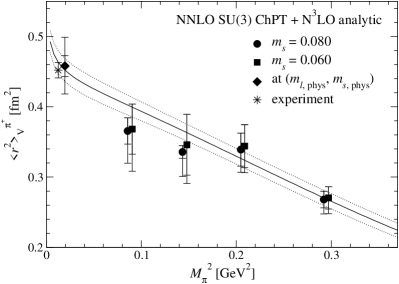
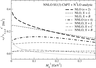
Figure 30: Left panel: pion charge radius ${\langle r^{2}\rangle_{V}^{\pi^{+}}}$ as a function of $M_{\pi}^{2}$. The solid line represents ${\langle r^{2}\rangle_{V}^{\pi^{+}}}$ at $m_{s}\!=\!0.080$ reproduced from our chiral fit based on NNLO SU(3) ChPT. We plot the value extrapolated to the physical point by the diamond. The circles and squares are our estimate at simulation points listed in Table 10. The experimental value is plotted by the star. Right panel: NLO and NNLO LEC-(in)dependent contributions to ${\langle r^{2}\rangle_{V}^{\pi^{+}}}$.

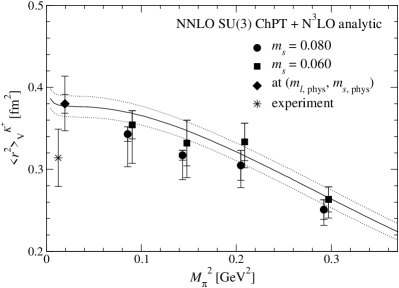
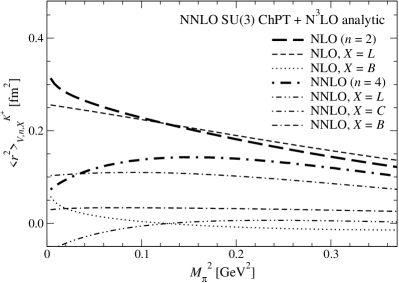
Figure 31: Same as Fig. 30, but for $F_{V}^{K^{+}}$.

The chiral extrapolation of the pion charge radius ${\langle r^{2}\rangle_{V}^{\pi^{+}}}$ is shown in the left panel of Fig. 30. In Subsection III.2, we estimate ${\langle r^{2}\rangle_{V}^{\pi^{+}}}$ at the simulation points by assuming the phenomenological $t$ dependence Eq. (36). These values are reproduced by our simultaneous chiral fit of $F_{V}^{\{\pi^{+},K^{+},K^{0}\}}$ reasonably well. This does not necessarily hold true: the non-analytic chiral behavior of $F_{V}^{\pi^{+}}$ may not be well described by our simple assumption (36), which is essentially low-order polynomial in $t$ in our region $|t|\!\ll\!M_{\rho}^{2}$. The reasonable consistency is partly because $F_{V}^{\pi^{+}}$ is largely dominated by the analytic terms $F_{V,2,L}^{\pi^{+}}\!+\!F_{V,4,C}^{\pi^{+}}$. In fact, the right panel of the same figure shows that ${\langle r^{2}\rangle_{V}^{\pi^{+}}}$ is also dominated by the analytic terms ${\langle r^{2}\rangle_{V,2,L}^{\pi^{+}}}\!+\!{\langle r^{2}\rangle_{V,4,C}^{\pi^{+}}}$. This supports our strategy of the chiral fit: namely, we determine $L_{9}^{r}$ and $O(p^{6})$ couplings appearing in these large analytic terms from our simulations, whereas other $L_{i}^{r}$’s in the small loop corrections are fixed to the phenomenological estimate.

More importantly, the value extrapolated to the physical point is in excellent agreement with the experimental value. The enhancement of the NLO chiral logarithm is important for this agreement. It is however partly compensated by the decrease of the NNLO contribution, similar to the analysis in SU(2) ChPT. The logarithmic singularity is therefore difficult to directly observe at our simulation region of $M_{\pi}\!\gtrsim\!300$ MeV.

Also for the charged kaon radius, we observe good agreement between simulation results and the experimental value ${\langle r^{2}\rangle_{V}^{K^{+}}}\!=\!0.314(35)~{}\mbox{fm}^{2}$ PDG:2014 as plotted in the left panel of Fig. 31. A comparison of the right panels of Figs. 30 and 31 suggests that the difference between ${\langle r^{2}\rangle_{V}^{K^{+}}}$ and ${\langle r^{2}\rangle_{V}^{\pi^{+}}}$ is mainly due to the suppression of the NLO chiral logarithms in Eqs. (90) – (91), and because the NNLO term $F_{V,4,L}^{K^{+}}$ becomes negative near the physical point with our choice of the input $L_{\{1,\cdots,5\}}^{r}$.

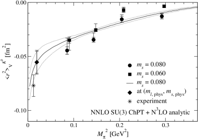
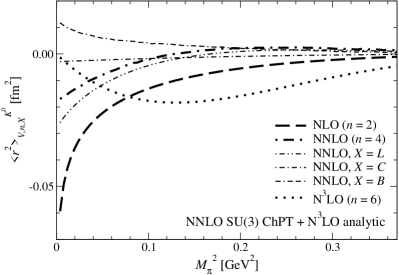
Figure 32: Same as Fig. 30, but for $F_{V}^{K^{0}}$.

Our chiral extrapolation also reproduces the experimental value of the neutral kaon radius ${\langle r^{2}\rangle_{V}^{K^{0}}}\!=\!-0.077(10)~{}\mbox{fm}^{2}$ as shown in Fig. 32. Similar to $F_{V}^{K^{0}}$, the parameter-free leading term ${\langle r^{2}\rangle_{V,2}^{K^{0}}}$ becomes the largest contribution only at small pion masses $M_{\pi}\!\lesssim\!300$ MeV. As already mentioned, the pion radius ${\langle r^{2}\rangle_{V}^{\pi^{+}}}$ is considered as a good quantity to observe the one-loop chiral logarithm. We note that ${\langle r^{2}\rangle_{V}^{K^{0}}}$ does not have analytic term at this order (${\langle r^{2}\rangle_{V,2,L}^{K^{0}}}\!=\!0$) and could be another good candidate provided that one simulates $M_{\pi}$ below 300 MeV with $m_{s}$ held fixed at a rather heavier value.

Since we simulate at a single lattice spacing, we assign the discretization error to our numerical results by an order counting $O((a\Lambda_{\rm QCD})^{2})\!\sim\!8$ %. At the renormalization scale $\mu\!=\!M_{\rho}$, we obtain

$$L_{9}^{r} = 4.6(1.1)\left({}^{+0.1}_{-0.5}\right)(0.4)\times 10^{-3},$$ (97)

$${c_{t^{2}}^{r}} = -6.4(1.1)(0.1)(0.5)\times 10^{-5}.$$ (98)

These are in good agreement with $L_{9}^{r}\!=\!5.9(0.4)\!\times\!10^{-3}$ and ${c_{t^{2}}^{r}}\!=\!C_{88}^{r}\!-\!C_{90}^{r}\!=\!-5.5(0.5)\!\times\!10^{5}$ obtained from a phenomenological analysis of the experimental data of $F_{V}^{\pi^{+}}$ in NNLO SU(3) ChPT PFF+KFF:ChPT:NNLO:Nf3 . Other $O(p^{6})$ couplings

$${c_{\pi^{+},\pi t}^{r}} = -1.95(84)\left({}^{+38}_{-21}\right)(16)\times 10^{-5},$$ (99)

$${c_{\pi^{+},Kt}^{r}} = -1.4(1.2)\left({}^{+0.1}_{-0.7}\right)(0.1)\times 10^{-5},$$ (100)

$${c_{K^{+},\pi t}^{r}} = -1.3(1.2)\left({}^{+0.1}_{-0.7}\right)(0.1)\times 10^{-5},$$ (101)

$$c_{K^{+},Kt}^{r} = -3.4(1.9)\left({}^{+0.1}_{-0.3}\right)(0.3)\times 10^{-5},$$ (102)

$${c_{K^{0}}^{r}} = 0.15(62)\left({}^{+12}_{-7}\right)(1)\times 10^{-5},$$ (103)

are poorly known phenomenologically, and we obtain

$${d_{K^{0}}} = -37(12)(2)(3)\times 10^{-7}$$ (104)

for the coefficient of the higher order correction to $F_{V}^{K^{0}}$. Our numerical results for the light meson charge radii

$${\langle r^{2}\rangle_{V}^{\pi^{+}}} = 0.458(15)\left({}^{+9}_{-1}\right)(37)~{}\mbox{fm}^{2},$$ (105)

$${\langle r^{2}\rangle_{V}^{K^{+}}} = 0.380(12)\left({}^{+7}_{-1}\right)(31)~{}\mbox{fm}^{2},$$ (106)

$${\langle r^{2}\rangle_{V}^{K^{0}}} = -0.055(10)(1)(4)~{}\mbox{fm}^{2}$$ (107)

are in reasonable agreement with experiment.

VI Conclusions

In this article, we have presented our detailed study of the chiral behavior of the light meson EM form factors. Chiral symmetry is exactly preserved in our simulations for a direct comparison with continuum ChPT at NNLO. Another salient feature is that we precisely calculate the EM form factors by using the all-to-all quark propagator.

Our analyses in SU(2) and SU(3) ChPT suggest reasonable convergence of the NNLO chiral expansion of the charged meson EM form factors $F_{V}^{\{\pi^{+},K^{+}\}}$. This is mainly because the non-trivial correction $F_{V}^{\{\pi^{+},K^{+}\}}-1$ is largely dominated by the NLO analytic term, which mildly depends on the quark masses. This term however vanishes in the neutral kaon form factor $F_{V}^{K^{0}}$. Although the corresponding chiral expansion shows poorer convergence at our simulated pion masses $M_{\pi}\!\gtrsim\!300$ MeV, it is rapidly improved towards the physical pion mass.

The NNLO tree diagrams with the $O(p^{6})$ couplings also tend to compose of a large part of the NNLO contribution. We observe small but non-negligible loop corrections, which have non-analytic dependence on the quark masses and momentum transfer. These confirm the importance of the first-principle determination of the relevant LECs based on the NNLO ChPT.

Our results for the LECs $\bar{l}_{6}^{r}$, $L_{9}^{r}$ and ${c_{t^{2}}^{r}}\!=\!C_{88}^{r}\!-\!C_{90}^{r}$ are consistent with the phenomenological estimates. We also observe a reasonable agreement of the charge radii with experiment.

Our results for the phenomenologically poorly-known $O(p^{6})$ couplings would be useful for studying different observables based on ChPT. An interesting application is the form factor of the $K\!\to\!\pi l\nu$ semileptonic decays, since its vector form factor $f_{+}^{K\pi}(t)$ shares many $O(p^{6})$ couplings with the EM form factors KFF:weak:ChPT:SU3:NNLO:BT . These decays provide a precise determination of the CKM matrix element $|V_{us}|$ through a precision lattice calculation of the normalization $f_{+}^{K\pi}(0)$. A comparison of the form factor shape with experiment can demonstrate the reliability of such a precise calculation. Our results of the LECs may enable us to study the normalization and shape simultaneously based on NNLO SU(3) ChPT.

Our analysis suggests that the charge radii show the one-loop chiral logarithm below $M_{\pi}\!\approx\!300$ MeV. Pushing simulations towards such small pion masses is interesting for unambiguous observation of the logarithmic singularity in QCD. Extension towards finer lattices is also important, because the largest uncertainty in our numerical results is the discretization error. Simulations in these directions are underway JLQCD:Noaki:Lat14 by using a computationally cheaper fermion formulation with good chiral symmetry JLQCD:TK:Lat15 .

Appendix A One-loop integrals in SU(3) ChPT

We summarize the expression of the one-loop integral functions in SU(3) ChPT in this section, as well as the expressions of the two-loop integrals and relevant two-loop contributions to $F_{V}^{\pi^{+}}$ in Appendix B. We refer to the original papers PFF+KFF:ChPT:NNLO:Nf3 ; Spec+DC:ChPT:SU3:NNLO:ABT for more detailed discussions.

The one-loop integral functions are defined as

$$A(M_{1}^{2}) = \frac{1}{i}\int\frac{d^{d}k}{(2\pi)^{d}}\frac{1}{k^{2}-M_{1}^{2}},$$ (108)

$$B(M_{1}^{2},M_{2}^{2},t) = \frac{1}{i}\int\frac{d^{d}k}{(2\pi)^{d}}\frac{1}{(k^{2}-M_{1}^{2})\left\{(k-q)^{2}-M_{2}^{2}\right\}},$$ (109)

$$B_{\mu}(M_{1}^{2},M_{2}^{2},t) = \frac{1}{i}\int\frac{d^{d}k}{(2\pi)^{d}}\frac{k_{\mu}}{(k^{2}-M_{1}^{2})\left\{(k-q)^{2}-M_{2}^{2}\right\}},$$ (110)

$$B_{\mu\nu}(M_{1}^{2},M_{2}^{2},t) = \frac{1}{i}\int\frac{d^{d}k}{(2\pi)^{d}}\frac{k_{\mu}k_{\nu}}{(k^{2}-M_{1}^{2})\left\{(k-q)^{2}-M_{2}^{2}\right\}},$$ (111)

$$B_{\mu\nu\alpha}(M_{1}^{2},M_{2}^{2},t) = \frac{1}{i}\int\frac{d^{d}k}{(2\pi)^{d}}\frac{k_{\mu}k_{\nu}k_{\alpha}}{(k^{2}-M_{1}^{2})\left\{(k-q)^{2}-M_{2}^{2}\right\}},$$ (112)

where $q^{2}\!=\!t$ and $d\!=\!4-2\epsilon$. The scalar function $A$ is needed to evaluate diagrams such as shown in Fig. 33 – 1, and hence does not depend on $t$. The $t$-dependent “$B$” functions are needed for Fig. 33 – 2.

Figure 33: Example of one-loop diagrams involving momentum-transfer independent (1) and dependent loop integrals (2).

The Lorentz decomposition of the vector and tensor functions is given as

$$B_{\mu}(M_{1}^{2},M_{2}^{2},t) = q_{\mu}B_{1}(M_{1}^{2},M_{2}^{2},t),$$ (113)

$$B_{\mu\nu}(M_{1}^{2},M_{2}^{2},t) = q_{\mu}q_{\nu}B_{21}(M_{1}^{2},M_{2}^{2},t)+g_{\mu\nu}B_{22}(M_{1}^{2},M_{2}^{2},t),$$ (114)

$$B_{\mu\nu\alpha}(M_{1}^{2},M_{2}^{2},t) = q_{\mu}q_{\nu}q_{\alpha}B_{31}(M_{1}^{2},M_{2}^{2},t)$$ (115)

$$\hskip 14.22636pt+\left(q_{\mu}g_{\nu\alpha}+q_{\nu}g_{\alpha\mu}+q_{\alpha}g_{\mu\nu}\right)B_{32}(M_{1}^{2},M_{2}^{2},t).$$

The “$B$” functions in the right hand side are expressed in terms of the scalar functions $A$ and $B$

$$B_{1}(M_{1}^{2},M_{2}^{2},t) = \frac{1}{2t}\left\{-A(M_{1}^{2})+A(M_{2}^{2})+(\Delta_{12}+t)B(M_{1}^{2},M_{2}^{2},t)\right\},$$ (116)

$$B_{21}(M_{1}^{2},M_{2}^{2},t) = \frac{1}{t}\left\{A(M_{2}^{2})+M_{1}^{2}B(M_{1}^{2},M_{2}^{2},t)-dB_{22}(M_{1}^{2},M_{2}^{2},t)\right\},$$ (117)

$$B_{22}(M_{1}^{2},M_{2}^{2},t) = \frac{1}{2(d-1)}\left\{A(M_{2}^{2})+2M_{1}^{2}B(M_{1}^{2},M_{2}^{2},t)\right.$$ (118)

$$\hskip 170.71652pt\left.-(\Delta_{12}+t)B_{1}(M_{1}^{2},M_{2}^{2},t)\right\},$$

$$B_{31}(M_{1}^{2},M_{2}^{2},t) = \frac{1}{2t}\left\{A(M_{2}^{2})+(\Delta_{12}+t)B_{21}(M_{1}^{2},M_{2}^{2},t)-4B_{32}(M_{1}^{2},M_{2}^{2},t)\right\},$$ (119)

$$B_{32}(M_{1}^{2},M_{2}^{2},t) = \frac{1}{2dt}\left\{-M_{1}^{2}A(M_{1}^{2})+M_{2}^{2}A(M_{2}^{2})+d(\Delta_{12}+t)B_{22}(M_{1}^{2},M_{2}^{2},t)\right\}\hskip 56.9055pt$$ (120)

with $\Delta_{12}=M_{1}^{2}-M_{2}^{2}$. The pole, finite and $O(\epsilon)$ parts of the one-loop integrals relevant to the EM form factors can be expressed in terms of those of $A$ and $B$ functions

$$A(M_{1})^{2} = A_{\rm pole}(M_{1}^{2})+\bar{A}(M_{1}^{2})+\epsilon\bar{A}^{\epsilon}(M_{1}^{2})+O(\epsilon^{2}),$$ (121)

$$B(M_{1}^{2},M_{2}^{2},t) = B_{\rm pole}(M_{1}^{2},M_{2}^{2},t)+\bar{B}(M_{1}^{2},M_{2}^{2},t)+\epsilon\bar{B}^{\epsilon}(M_{1}^{2},M_{2}^{2},t)+O(\epsilon^{2})\vspace{20mm}$$ (122)

with

$$A_{\rm pole}(M_{1}^{2}) = \frac{M_{1}^{2}}{N}\lambda_{0},$$ (123)

$$\bar{A}(M_{1}^{2}) = -\frac{M_{1}^{2}}{N}\ln\left[\frac{M_{1}^{2}}{\mu^{2}}\right],$$ (124)

$$\bar{A}^{\epsilon}(M_{1}^{2}) = \frac{M_{1}^{2}}{N}\left\{\frac{C^{2}}{2}+\frac{1}{2}+\frac{\pi^{2}}{12}+\frac{1}{2}\ln^{2}\left[\frac{M_{1}^{2}}{\mu^{2}}\right]-C\ln\left[\frac{M_{1}^{2}}{\mu^{2}}\right]\right\},$$ (125)

$$B_{\rm pole}(M_{1}^{2},M_{2}^{2},t) = \frac{1}{N}\lambda_{0},$$ (126)

$$\bar{B}(M_{1}^{2},M_{2}^{2},t) = -\frac{1}{N}\frac{M_{1}^{2}\ln\left[\frac{M_{1}^{2}}{\mu^{2}}\right]+M_{2}^{2}\ln\left[\frac{M_{2}^{2}}{\mu^{2}}\right]}{\Delta_{12}}$$ (127)

$$+\frac{1}{2N}\left\{2+\left(-\frac{\Delta_{12}}{t}+\frac{\Sigma_{12}}{\Delta_{12}}\right)\ln\left[\frac{M_{1}^{2}}{M_{2}^{2}}\right]\right.$$

$$\hskip 113.81102pt\left.-\frac{\nu_{12}(t)}{t}\ln\left[\frac{(t+\nu_{12}(t))^{2}-\Delta_{12}^{2}}{(t-\nu_{12}(t))^{2}-\Delta_{12}^{2}}\right]\right\},$$

$$\bar{B}^{\epsilon}(M_{1}^{2},M_{2}^{2},t) = \frac{1}{N}\left\{\frac{C^{2}}{2}-\frac{1}{2}+\frac{\pi^{2}}{12}+(C-1)\bar{B}(M_{1}^{2},M_{2}^{2},t)\right.$$ (128)

$$\hskip 56.9055pt\left.+\frac{1}{2}\int_{0}^{1}dx\ln^{2}\left[\frac{xM_{1}^{2}+(1-x)M_{2}^{2}-x(1-x)t}{\mu^{2}}\right]\right\},\hskip 28.45274pt$$

where

$$\Sigma_{12} = M_{1}^{2}+M_{2}^{2},$$ (129)

$$\nu_{12}^{2} = t^{2}-2\Sigma_{12}t+\Delta_{12}^{2},$$ (130)

$$\lambda_{0} = \frac{1}{\epsilon}+\ln\left[4\pi\right]+1-\gamma=\frac{1}{\epsilon}+C.$$ (131)

The one-loop contributions in Eqs. (69) – (71) are expressed in terms of the finite parts $\bar{A}$ and $\bar{B}_{22}$.

Appendix B Two-loop integrals in SU(3) ChPT

We categorize the two-loop diagrams into three types: those with the reducible, sunset and vertex integrals. An example is shown in Fig. 34.

Figure 34: Example of two-loop diagrams with reducible (1), sunset (2), and vertex integrals (3).

B.1 Diagrams with reducible integral

The diagram of Fig. 34 – 1 involves two independent one-loop integrals. The contribution of this type of diagram can be written in terms of the one-loop integral functions discussed in Appendix A. The expression for the pion form factor is given by PFF+KFF:ChPT:NNLO:Nf3

$$F_{\pi}^{4}\,F_{V,4,B,{\rm reducible}}^{\pi^{+}}(t)$$ (132)

$$= \frac{1}{N}\left\{-\frac{1}{2}M_{\pi}^{2}{\bar{A}(M_{\pi}^{2})}-\frac{1}{4}M_{\pi}^{2}{\bar{A}(M_{K}^{2})}\right\}$$

$$+\frac{1}{N^{2}}\left\{-\frac{\pi^{2}}{48}M_{\pi}^{2}(10M_{\pi}^{2}+3M_{K}^{2})+\frac{35}{96}M_{\pi}^{2}(M_{\pi}^{2}-2M_{K}^{2})\right.$$

$$\hskip 199.16928pt\left.-\frac{89}{48}M_{\pi}^{4}-\frac{1}{16}\left(1+\frac{\pi^{2}}{6}\right)\,(2M_{\pi}^{2}+M_{K}^{2})\,t\right\}$$

$$+\frac{1}{N}\left(5M_{\pi}^{2}-\frac{t}{2}\right)\bar{B}_{22}^{\epsilon}(M_{\pi}^{2},M_{\pi}^{2},t)+\frac{1}{N}\left(\frac{3}{2}M_{\pi}^{2}-\frac{t}{4}\right)\bar{B}_{22}^{\epsilon}(M_{K}^{2},M_{K}^{2},t)$$

$$+4\left\{{\bar{B}_{22}(M_{\pi}^{2},M_{\pi}^{2},t)}\right\}^{2}+4{\bar{B}_{22}(M_{\pi}^{2},M_{\pi}^{2},t)}{\bar{B}_{22}(M_{K}^{2},M_{K}^{2},t)}+\left\{{\bar{B}_{22}(M_{K}^{2},M_{K}^{2},t)}\right\}^{2}$$

$$-\left\{4{\bar{A}(M_{\pi}^{2})}+2{\bar{A}(M_{K}^{2})}\right\}{\bar{B}_{22}(M_{\pi}^{2},M_{\pi}^{2},t)}-\left\{2{\bar{A}(M_{\pi}^{2})}+{\bar{A}(M_{K}^{2})}\right\}{\bar{B}_{22}(M_{K}^{2},M_{K}^{2},t)}$$

$$-\frac{1}{4}\left\{{\bar{A}(M_{\pi}^{2})}\right\}^{2}+{\bar{A}(M_{\pi}^{2})}{\bar{A}(M_{K}^{2})}+\left(\frac{1}{4}-\frac{3}{8}\frac{M_{\pi}^{2}}{M_{K}^{2}}\right)\left\{{\bar{A}(M_{K}^{2})}\right\}^{2}$$

$$-\frac{1}{8}\frac{t}{M_{\pi}^{2}}\left\{{\bar{A}(M_{\pi}^{2})}\right\}^{2}-\frac{1}{16}\frac{t}{M_{K}^{2}}\left\{{\bar{A}(M_{K}^{2})}\right\}^{2}.$$

B.2 Diagrams with sunset integral

The diagram of Fig. 34 – 2 involves the so-called sunset integral, which is genuine two-loop integral. This type of integral is $t$-independent, and hence also appears in the two-loop chiral expansion of the meson masses and decay constants Spec+DC:ChPT:SU3:NNLO:ABT .

A typical form of the sunset integral is

$$\langle\langle X(r,s)\rangle\rangle_{\rm s} = \frac{1}{i^{2}}\int\frac{d^{2}r}{(2\pi)^{d}}\frac{d^{2}s}{(2\pi)^{d}}\frac{X(r,s)}{(r^{2}-M_{1}^{2})(s^{2}-M_{2}^{2})\left\{(p-r-s)^{2}-M_{3}^{2}\right\}},$$ (133)

where $X(r,s)$ specifies the tensor structure in terms of the loop momenta $r$ and $s$. We consider the following three integrals with $X(r,s)\!=\!1,r_{\mu},r_{\mu}r_{\nu}$

$$H(M_{1}^{2},M_{2}^{2},M_{3}^{2};p^{2}) = \langle\langle 1\rangle\rangle_{\rm s},$$ (134)

$$H_{\mu}(M_{1}^{2},M_{2}^{2},M_{3}^{2};p^{2}) = \langle\langle r_{\mu}\rangle\rangle_{\rm s},$$ (135)

$$H_{\mu\nu}(M_{1}^{2},M_{2}^{2},M_{3}^{2};p^{2}) = \langle\langle r_{\mu}r_{\nu}\rangle\rangle_{\rm s}.$$ (136)

By redefining the momenta, other sunset integrals with $X(r,s)\!=\!s_{\mu},s_{\mu}s_{\nu},r_{\mu}s_{\nu}$ can be related to the above three functions Spec+DC:ChPT:SU3:NNLO:ABT .

The Lorentz decomposition of these “$H$” functions is given as

$$H_{\mu}(M_{1}^{2},M_{2}^{2},M_{3}^{2};p^{2}) = p_{\mu}H_{1}(M_{1}^{2},M_{2}^{2},M_{3}^{2};p^{2}),$$ (137)

$$H_{\mu\nu}(M_{1}^{2},M_{2}^{2},M_{3}^{2};p^{2}) = p_{\mu}p_{\nu}H_{21}(M_{1}^{2},M_{2}^{2},M_{3}^{2};p^{2})+g_{\mu\nu}H_{22}(M_{1}^{2},M_{2}^{2},M_{3}^{2};p^{2}).$$ (138)

It is possible to express $H_{22}$ as PFF+KFF:ChPT:NNLO:Nf3

$$dH_{22}(M_{1}^{2},M_{2}^{2},M_{3}^{2};p^{2})$$ (139)

$$= -p^{2}H_{21}(M_{1}^{2},M_{2}^{2},M_{3}^{2};p^{2})+M_{1}^{2}H(M_{1}^{2},M_{2}^{2},M_{3}^{2};p^{2})+A(M_{2}^{2})A(M_{3}^{2}).$$

Therefore, the contribution of the sunset diagrams to $F_{V}^{\pi^{+}}$ can be calculated with $H_{X}(M_{1}^{2},M_{2}^{2},M_{3}^{2},p^{2})$ with $X\!=\!"",1,21$

$$F_{\pi}^{4}\,F_{V,4,{\rm sunset}}^{\pi^{+}}(t)$$

$$= \frac{3}{2}M_{\pi}^{4}H^{F\prime}(M_{\pi}^{2},M_{\pi}^{2},M_{\pi}^{2};M_{\pi}^{2})-\frac{5}{8}M_{\pi}^{4}H^{F\prime}(M_{\pi}^{2},M_{K}^{2},M_{K}^{2};M_{\pi}^{2})$$

$$+\frac{1}{18}M_{\pi}^{4}H^{F\prime}(M_{\pi}^{2},M_{\eta}^{2},M_{\eta}^{2};M_{\pi}^{2})+M_{\pi}^{2}M_{K}^{2}H^{F\prime}(M_{K}^{2},M_{\pi}^{2},M_{K}^{2};M_{\pi}^{2})$$

$$-\frac{5}{6}M_{\pi}^{4}H^{F\prime}(M_{K}^{2},M_{K}^{2},M_{\eta}^{2};M_{\pi}^{2})-\frac{1}{4}M_{\pi}^{2}\left(\frac{1}{2}M_{\pi}^{2}-2M_{K}^{2}\right)H^{F\prime}(M_{\eta}^{2},M_{K}^{2},M_{K}^{2};M_{\pi}^{2})$$

$$-2M_{\pi}^{4}H_{1}^{F\prime}(M_{\pi}^{2},M_{\pi}^{2},M_{\pi}^{2};M_{\pi}^{2})+M_{\pi}^{4}H_{1}^{F\prime}(M_{\pi}^{2},M_{K}^{2},M_{K}^{2};M_{\pi}^{2})$$

$$+2M_{\pi}^{4}H_{1}^{F\prime}(M_{K}^{2},M_{K}^{2},M_{\eta}^{2};M_{\pi}^{2})$$

$$+3M_{\pi}^{4}H_{21}^{F\prime}(M_{\pi}^{2},M_{\pi}^{2},M_{\pi}^{2};M_{\pi}^{2})-\frac{3}{8}M_{\pi}^{4}H_{21}^{F\prime}(M_{\pi}^{2},M_{K}^{2},M_{K}^{2};M_{\pi}^{2})$$

$$+3M_{\pi}^{4}H_{21}^{F\prime}(M_{K}^{2},M_{\pi}^{2},M_{K}^{2};M_{\pi}^{2})+\frac{9}{8}M_{\pi}^{4}H_{21}^{F\prime}(M_{\eta}^{2},M_{K}^{2},M_{K}^{2};M_{\pi}^{2})$$

$$+\left(\frac{5}{3}M_{\pi}^{2}+\frac{1}{18}t\right)H^{F}(M_{\pi}^{2},M_{\pi}^{2},M_{\pi}^{2};M_{\pi}^{2})+\frac{1}{12}(M_{\pi}^{2}+t)H^{F}(M_{\pi}^{2},M_{K}^{2},M_{K}^{2};M_{\pi}^{2})$$

$$+\left\{\frac{15}{32}M_{\pi}^{2}-\frac{5}{96}(M_{\pi}^{2}-2M_{K}^{2})-\frac{5}{48}t\right\}H^{F}(M_{K}^{2},M_{\pi}^{2},M_{K}^{2};M_{\pi}^{2})$$

$$-\frac{5}{48}M_{K}^{2}H^{F}(M_{K}^{2},M_{K}^{2},M_{\pi}^{2};M_{\pi}^{2})$$

$$-\left(\frac{1}{12}M_{\pi}^{2}+\frac{1}{16}t\right)H^{F}(M_{K}^{2},M_{K}^{2},M_{\eta}^{2};M_{\pi}^{2})$$

$$-\left(3M_{\pi}^{2}+\frac{1}{3}t\right)H_{1}^{F}(M_{\pi}^{2},M_{\pi}^{2},M_{\pi}^{2};M_{\pi}^{2})+\frac{1}{24}tH_{1}^{F}(M_{\pi}^{2},M_{K}^{2},M_{K}^{2};M_{\pi}^{2})$$

$$-\left(M_{\pi}^{2}+\frac{1}{8}t\right)H_{1}^{F}(M_{K}^{2},M_{\pi}^{2},M_{K}^{2};M_{\pi}^{2})+\left(M_{\pi}^{2}+\frac{1}{8}t\right)H_{1}^{F}(M_{K}^{2},M_{K}^{2},M_{\eta}^{2};M_{\pi}^{2})$$

$$+\left(3M_{\pi}^{2}+\frac{1}{6}t\right)H_{21}^{F}(M_{\pi}^{2},M_{\pi}^{2},M_{\pi}^{2};M_{\pi}^{2})-\left(\frac{3}{8}M_{\pi}^{2}+\frac{1}{48}t\right)H_{21}^{F}(M_{\pi}^{2},M_{K}^{2},M_{K}^{2};M_{\pi}^{2})$$

$$+\left(\frac{53}{16}M_{\pi}^{2}+\frac{1}{16}t\right)H_{21}^{F}(M_{K}^{2},M_{\pi}^{2},M_{K}^{2};M_{\pi}^{2})$$

$$-\left(\frac{5}{16}M_{\pi}^{2}-\frac{5}{48}t\right)H_{21}^{F}(M_{K}^{2},M_{K}^{2},M_{\pi}^{2};M_{\pi}^{2})$$

$$+\left(\frac{9}{8}M_{\pi}^{2}+\frac{1}{16}t\right)H_{21}^{F}(M_{\eta}^{2},M_{K}^{2},M_{K}^{2};M_{\pi}^{2}).$$ (140)

Here $H_{X}^{F}(M_{1}^{2},M_{2}^{2},M_{3}^{2};p^{2})$ and $H_{X}^{F\prime}(M_{1}^{2},M_{2}^{2},M_{3}^{2};p^{2})$ ($X\!=\!"",1,21$) represent the finite part of $H_{X}(M_{1}^{2},M_{2}^{2},M_{3}^{2};p^{2})$ and its derivative with respective to $p^{2}$. We refer to Ref. Spec+DC:ChPT:SU3:NNLO:ABT for the explicit expression of these “$H$” functions.

B.3 Diagrams with vertex integral

The vertex integral is $t$-dependent genuine two-loop integral involved in diagrams such as Fig. 34 – 3. It is defined as PFF+KFF:ChPT:NNLO:Nf3

$$\langle\langle X(r,s)\rangle\rangle_{\rm v}$$ (141)

$$= \frac{1}{i^{2}}\int\frac{d^{2}r}{(2\pi)^{d}}\frac{d^{2}s}{(2\pi)^{d}}\frac{X(r,s)}{(r^{2}-M_{1}^{2})\left\{(r-q)^{2}-M_{2}^{2}\right\}(s^{2}-M_{3}^{2})\left\{(p-r-s)^{2}-M_{4}^{2}\right\}}.\hskip 28.45274pt$$

The Lorentz decomposition of the vertex integrals can be expressed as

$$\langle\langle r_{\mu}\rangle\rangle_{\rm v} = p_{\mu}V_{1,1}+q_{\mu}V_{1,2},$$ (142)

$$\langle\langle r_{\mu}r_{\nu}\rangle\rangle_{\rm v} = g_{\mu\nu}V_{2,1}+p_{\mu}p_{\nu}V_{2,2}+q_{\mu}q_{\nu}V_{2,3}+(p_{\mu}q_{\nu}+q_{\mu}p_{\nu})V_{2,4},$$ (143)

$$\langle\langle r_{\mu}r_{\nu}r_{\alpha}\rangle\rangle_{\rm v} = (g_{\mu\nu}p_{\alpha}+g_{\nu\alpha}p_{\mu}+g_{\alpha\mu}p_{\nu})V_{3,1}+(g_{\mu\nu}q_{\alpha}+g_{\nu\alpha}q_{\mu}+g_{\alpha\mu}q_{\nu})V_{3,2}$$ (144)

$$+p_{\mu}p_{\nu}p_{\alpha}V_{3,3}+q_{\mu}q_{\nu}q_{\alpha}V_{3,4}+(p_{\mu}p_{\nu}q_{\alpha}+p_{\mu}q_{\nu}p_{\alpha}+q_{\mu}p_{\nu}p_{\alpha})V_{3,5}\hskip 14.22636pt$$

$$+(p_{\mu}q_{\nu}q_{\alpha}+q_{\mu}p_{\nu}q_{\alpha}+q_{\mu}q_{\nu}p_{\alpha})V_{3,6}$$

using the integral functions $V_{i,j}(M_{1}^{2},M_{2}^{2},M_{3}^{2},M_{4}^{2};p^{2},q^{2},(p-q)^{2})$, where $i$ represents the number of the momentum appearing in $X(r,s)$ and $j$ is the index of the integral function for a given $i$. For $i\!\leq\!3$, there exist 44 scalar functions with

$$(i,j) = (0,0),\hskip 5.69054pt(1,1),\ldots,(1,4),\hskip 5.69054pt(2,1),\ldots,(2,13),\hskip 5.69054pt(3,1),\ldots,(3,26).$$ (145)

The explicit expression of these ”$V$” functions is given in Ref. PFF+KFF:ChPT:NNLO:Nf3 . The two-loop contribution to $F_{V}^{\pi^{+}}$ with the vertex integral can be written with a subset of these functions in a rather involved form:

$$F_{\pi}^{4}\,F_{V,4,{\rm vertex}}^{\pi^{+}}(t)$$

$$= \left(\frac{5}{2}M_{\pi}^{4}-\frac{7}{3}M_{\pi}^{2}t\right)V_{1,1}(M_{\pi}^{2},M_{\pi}^{2},M_{\pi}^{2},M_{\pi}^{2};M_{\pi}^{2},t,M_{\pi}^{2})$$

$$+\left(M_{\pi}^{4}-\frac{2}{3}M_{\pi}^{2}t+\frac{1}{12}t^{2}\right)V_{1,1}(M_{\pi}^{2},M_{\pi}^{2},M_{K}^{2},M_{K}^{2};M_{\pi}^{2},t,M_{\pi}^{2})$$

$$+\frac{1}{18}M_{\pi}^{4}V_{1,1}(M_{\pi}^{2},M_{\pi}^{2},M_{\eta}^{2},M_{\eta}^{2};M_{\pi}^{2},t,M_{\pi}^{2})$$

$$+\left(\frac{3}{2}M_{\pi}^{4}-\frac{17}{12}M_{\pi}^{2}t+\frac{1}{6}t^{2}\right)V_{1,1}(M_{K}^{2},M_{K}^{2},M_{\pi}^{2},M_{K}^{2};M_{\pi}^{2},t,M_{\pi}^{2})$$

$$+\left(\frac{2}{3}M_{\pi}^{4}-\frac{2}{3}M_{\pi}^{2}t+\frac{1}{8}t^{2}\right)V_{1,1}(M_{K}^{2},M_{K}^{2},M_{K}^{2},M_{\eta}^{2};M_{\pi}^{2},t,M_{\pi}^{2})$$

$$+\left(-6M_{\pi}^{2}+t\right)V_{2,1}(M_{\pi}^{2},M_{\pi}^{2},M_{\pi}^{2},M_{\pi}^{2};M_{\pi}^{2},t,M_{\pi}^{2})$$

$$+\left(-2M_{\pi}^{2}+\frac{2}{3}t\right)V_{2,1}(M_{\pi}^{2},M_{\pi}^{2},M_{K}^{2},M_{K}^{2};M_{\pi}^{2},t,M_{\pi}^{2})$$

$$+\left(-4M_{\pi}^{2}+\frac{4}{3}t\right)V_{2,1}(M_{K}^{2},M_{K}^{2},M_{\pi}^{2},M_{K}^{2};M_{\pi}^{2},t,M_{\pi}^{2})$$

$$+\left(-2M_{\pi}^{2}+t\right)V_{2,1}(M_{K}^{2},M_{K}^{2},M_{K}^{2},M_{\eta}^{2};M_{\pi}^{2},t,M_{\pi}^{2})$$

$$+\left(-6M_{\pi}^{4}+\frac{10}{3}M_{\pi}^{2}t\right)V_{2,2}(M_{\pi}^{2},M_{\pi}^{2},M_{\pi}^{2},M_{\pi}^{2};M_{\pi}^{2},t,M_{\pi}^{2})$$

$$+\left(-2M_{\pi}^{4}+\frac{4}{3}M_{\pi}^{2}t-\frac{1}{6}t^{2}\right)V_{2,2}(M_{\pi}^{2},M_{\pi}^{2},M_{K}^{2},M_{K}^{2};M_{\pi}^{2},t,M_{\pi}^{2})$$

$$+\left(-4M_{\pi}^{4}+\frac{11}{4}M_{\pi}^{2}t-\frac{1}{3}t^{2}\right)V_{2,2}(M_{K}^{2},M_{K}^{2},M_{\pi}^{2},M_{K}^{2};M_{\pi}^{2},t,M_{\pi}^{2})$$

$$+\left(-2M_{\pi}^{4}+\frac{5}{3}M_{\pi}^{2}t-\frac{1}{4}t^{2}\right)V_{2,2}(M_{K}^{2},M_{K}^{2},M_{K}^{2},M_{\eta}^{2};M_{\pi}^{2},t,M_{\pi}^{2})$$

$$+\left(\frac{5}{3}M_{\pi}^{2}t+\frac{1}{2}t^{2}\right)V_{2,4}(M_{\pi}^{2},M_{\pi}^{2},M_{\pi}^{2},M_{\pi}^{2};M_{\pi}^{2},t,M_{\pi}^{2})$$

$$+\frac{1}{3}M_{\pi}^{2}tV_{2,4}(M_{\pi}^{2},M_{\pi}^{2},M_{K}^{2},M_{K}^{2};M_{\pi}^{2},t,M_{\pi}^{2})+\frac{5}{6}M_{\pi}^{2}tV_{2,4}(M_{K}^{2},M_{K}^{2},M_{\pi}^{2},M_{K}^{2};M_{\pi}^{2},t,M_{\pi}^{2})$$

$$+\frac{1}{3}M_{\pi}^{2}tV_{2,4}(M_{K}^{2},M_{K}^{2},M_{K}^{2},M_{\eta}^{2};M_{\pi}^{2},t,M_{\pi}^{2})$$

$$+\left(-4M_{\pi}^{2}+\frac{4}{3}t\right)V_{2,5}(M_{\pi}^{2},M_{\pi}^{2},M_{\pi}^{2},M_{\pi}^{2};M_{\pi}^{2},t,M_{\pi}^{2})$$

$$+\left(-2M_{\pi}^{2}+\frac{1}{2}t\right)V_{2,5}(M_{\pi}^{2},M_{\pi}^{2},M_{K}^{2},M_{K}^{2};M_{\pi}^{2},t,M_{\pi}^{2})$$

$$+\left(-3M_{\pi}^{2}+\frac{17}{12}t\right)V_{2,5}(M_{K}^{2},M_{K}^{2},M_{\pi}^{2},M_{K}^{2};M_{\pi}^{2},t,M_{\pi}^{2})$$

$$+\left(-2M_{\pi}^{2}+t\right)V_{2,5}(M_{K}^{2},M_{K}^{2},M_{K}^{2},M_{\eta}^{2};M_{\pi}^{2},t,M_{\pi}^{2})$$

$$+\left(-4M_{\pi}^{4}+\frac{7}{3}M_{\pi}^{2}t+\frac{1}{3}t^{2}\right)V_{2,6}(M_{\pi}^{2},M_{\pi}^{2},M_{\pi}^{2},M_{\pi}^{2};M_{\pi}^{2},t,M_{\pi}^{2})$$

$$+\left(-2M_{\pi}^{4}+M_{\pi}^{2}t\right)V_{2,6}(M_{\pi}^{2},M_{\pi}^{2},M_{K}^{2},M_{K}^{2};M_{\pi}^{2},t,M_{\pi}^{2})$$

$$+\left(-3M_{\pi}^{4}+\frac{13}{6}M_{\pi}^{2}t-\frac{5}{24}t^{2}\right)V_{2,6}(M_{K}^{2},M_{K}^{2},M_{\pi}^{2},M_{K}^{2};M_{\pi}^{2},t,M_{\pi}^{2})$$

$$+\left(-2M_{\pi}^{4}+\frac{3}{2}M_{\pi}^{2}t-\frac{1}{8}t^{2}\right)V_{2,6}(M_{K}^{2},M_{K}^{2},M_{K}^{2},M_{\eta}^{2};M_{\pi}^{2},t,M_{\pi}^{2})$$

$$+\frac{4}{3}t^{2}V_{2,9}(M_{\pi}^{2},M_{\pi}^{2},M_{\pi}^{2},M_{\pi}^{2};M_{\pi}^{2},t,M_{\pi}^{2})+\frac{1}{4}t^{2}V_{2,9}(M_{\pi}^{2},M_{\pi}^{2},M_{K}^{2},M_{K}^{2};M_{\pi}^{2},t,M_{\pi}^{2})$$

$$+\frac{7}{24}t^{2}V_{2,9}(M_{K}^{2},M_{K}^{2},M_{\pi}^{2},M_{K}^{2};M_{\pi}^{2},t,M_{\pi}^{2})+\frac{1}{4}t^{2}V_{2,9}(M_{K}^{2},M_{K}^{2},M_{K}^{2},M_{\eta}^{2};M_{\pi}^{2},t,M_{\pi}^{2})$$

$$+\left(6M_{\pi}^{2}-2t\right)V_{3,1}(M_{\pi}^{2},M_{\pi}^{2},M_{\pi}^{2},M_{\pi}^{2};M_{\pi}^{2},t,M_{\pi}^{2})$$

$$+\left(3M_{\pi}^{2}-t\right)V_{3,1}(M_{\pi}^{2},M_{\pi}^{2},M_{K}^{2},M_{K}^{2};M_{\pi}^{2},t,M_{\pi}^{2})$$

$$+\left(6M_{\pi}^{2}-2t\right)V_{3,1}(M_{K}^{2},M_{K}^{2},M_{\pi}^{2},M_{K}^{2};M_{\pi}^{2},t,M_{\pi}^{2})$$

$$+\left(\frac{9}{2}M_{\pi}^{2}-\frac{3}{2}t\right)V_{3,1}(M_{K}^{2},M_{K}^{2},M_{K}^{2},M_{\eta}^{2};M_{\pi}^{2},t,M_{\pi}^{2})$$

$$-\frac{1}{3}tV_{3,2}(M_{\pi}^{2},M_{\pi}^{2},M_{K}^{2},M_{K}^{2};M_{\pi}^{2},t,M_{\pi}^{2})-\frac{2}{3}tV_{3,2}(M_{K}^{2},M_{K}^{2},M_{\pi}^{2},M_{K}^{2};M_{\pi}^{2},t,M_{\pi}^{2})$$

$$-\frac{1}{2}tV_{3,2}(M_{K}^{2},M_{K}^{2},M_{K}^{2},M_{\eta}^{2};M_{\pi}^{2},t,M_{\pi}^{2})$$

$$+\left(2M_{\pi}^{4}-M_{\pi}^{2}t\right)V_{3,3}(M_{\pi}^{2},M_{\pi}^{2},M_{\pi}^{2},M_{\pi}^{2};M_{\pi}^{2},t,M_{\pi}^{2})$$

$$+\left(M_{\pi}^{4}-\frac{2}{3}M_{\pi}^{2}t+\frac{1}{12}t^{2}\right)V_{3,3}(M_{\pi}^{2},M_{\pi}^{2},M_{K}^{2},M_{K}^{2};M_{\pi}^{2},t,M_{\pi}^{2})$$

$$+\left(2M_{\pi}^{4}-\frac{4}{3}M_{\pi}^{2}t+\frac{1}{6}t^{2}\right)V_{3,3}(M_{K}^{2},M_{K}^{2},M_{\pi}^{2},M_{K}^{2};M_{\pi}^{2},t,M_{\pi}^{2})$$

$$+\left(\frac{3}{2}M_{\pi}^{4}-M_{\pi}^{2}t+\frac{1}{8}t^{2}\right)V_{3,3}(M_{K}^{2},M_{K}^{2},M_{K}^{2},M_{\eta}^{2};M_{\pi}^{2},t,M_{\pi}^{2})$$

$$-\frac{1}{2}t^{2}V_{3,5}(M_{\pi}^{2},M_{\pi}^{2},M_{\pi}^{2},M_{\pi}^{2};M_{\pi}^{2},t,M_{\pi}^{2})-\frac{1}{3}M_{\pi}^{2}tV_{3,5}(M_{\pi}^{2},M_{\pi}^{2},M_{K}^{2},M_{K}^{2};M_{\pi}^{2},t,M_{\pi}^{2})$$

$$-\frac{2}{3}M_{\pi}^{2}tV_{3,5}(M_{K}^{2},M_{K}^{2},M_{\pi}^{2},M_{K}^{2};M_{\pi}^{2},t,M_{\pi}^{2})-\frac{1}{2}M_{\pi}^{2}tV_{3,5}(M_{K}^{2},M_{K}^{2},M_{K}^{2},M_{\eta}^{2};M_{\pi}^{2},t,M_{\pi}^{2})$$

$$-\frac{1}{2}t^{2}V_{3,6}(M_{\pi}^{2},M_{\pi}^{2},M_{\pi}^{2},M_{\pi}^{2};M_{\pi}^{2},t,M_{\pi}^{2})-\frac{1}{12}t^{2}V_{3,6}(M_{\pi}^{2},M_{\pi}^{2},M_{K}^{2},M_{K}^{2};M_{\pi}^{2},t,M_{\pi}^{2})$$

$$-\frac{1}{6}t^{2}V_{3,6}(M_{K}^{2},M_{K}^{2},M_{\pi}^{2},M_{K}^{2};M_{\pi}^{2},t,M_{\pi}^{2})-\frac{1}{8}t^{2}V_{3,6}(M_{K}^{2},M_{K}^{2},M_{K}^{2},M_{\eta}^{2};M_{\pi}^{2},t,M_{\pi}^{2})$$

$$+4M_{\pi}^{2}V_{3,7}(M_{\pi}^{2},M_{\pi}^{2},M_{\pi}^{2},M_{\pi}^{2};M_{\pi}^{2},t,M_{\pi}^{2})$$

$$+\left(2M_{\pi}^{2}-\frac{1}{2}t\right)V_{3,7}(M_{\pi}^{2},M_{\pi}^{2},M_{K}^{2},M_{K}^{2};M_{\pi}^{2},t,M_{\pi}^{2})$$

$$+\left(4M_{\pi}^{2}-t\right)V_{3,7}(M_{K}^{2},M_{K}^{2},M_{\pi}^{2},M_{K}^{2};M_{\pi}^{2},t,M_{\pi}^{2})$$

$$+\left(3M_{\pi}^{2}-\frac{3}{4}t\right)V_{3,7}(M_{K}^{2},M_{K}^{2},M_{K}^{2},M_{\eta}^{2};M_{\pi}^{2},t,M_{\pi}^{2})$$

$$+2tV_{3,8}(M_{\pi}^{2},M_{\pi}^{2},M_{\pi}^{2},M_{\pi}^{2};M_{\pi}^{2},t,M_{\pi}^{2})$$

$$+\left(8M_{\pi}^{2}-4t\right)V_{3,9}(M_{\pi}^{2},M_{\pi}^{2},M_{\pi}^{2},M_{\pi}^{2};M_{\pi}^{2},t,M_{\pi}^{2})$$

$$+\left(4M_{\pi}^{2}-\frac{3}{2}t\right)V_{3,9}(M_{\pi}^{2},M_{\pi}^{2},M_{K}^{2},M_{K}^{2};M_{\pi}^{2},t,M_{\pi}^{2})$$

$$+\left(8M_{\pi}^{2}-3t\right)V_{3,9}(M_{K}^{2},M_{K}^{2},M_{\pi}^{2},M_{K}^{2};M_{\pi}^{2},t,M_{\pi}^{2})$$

$$+\left(6M_{\pi}^{2}-\frac{9}{4}t\right)V_{3,9}(M_{K}^{2},M_{K}^{2},M_{K}^{2},M_{\eta}^{2};M_{\pi}^{2},t,M_{\pi}^{2})$$

$$-\frac{2}{3}tV_{3,10}(M_{\pi}^{2},M_{\pi}^{2},M_{\pi}^{2},M_{\pi}^{2};M_{\pi}^{2},t,M_{\pi}^{2})-\frac{5}{6}tV_{3,10}(M_{K}^{2},M_{K}^{2},M_{\pi}^{2},M_{K}^{2};M_{\pi}^{2},t,M_{\pi}^{2})$$

$$-\frac{1}{2}tV_{3,10}(M_{K}^{2},M_{K}^{2},M_{K}^{2},M_{\eta}^{2};M_{\pi}^{2},t,M_{\pi}^{2})$$

$$+\left(4M_{\pi}^{4}-\frac{4}{3}M_{\pi}^{2}t-\frac{1}{3}t^{2}\right)V_{3,11}(M_{\pi}^{2},M_{\pi}^{2},M_{\pi}^{2},M_{\pi}^{2};M_{\pi}^{2},t,M_{\pi}^{2})$$

$$+\left(2M_{\pi}^{4}-M_{\pi}^{2}t\right)V_{3,11}(M_{\pi}^{2},M_{\pi}^{2},M_{K}^{2},M_{K}^{2};M_{\pi}^{2},t,M_{\pi}^{2})$$

$$+\left(4M_{\pi}^{4}-\frac{29}{12}M_{\pi}^{2}t+\frac{5}{24}t^{2}\right)V_{3,11}(M_{K}^{2},M_{K}^{2},M_{\pi}^{2},M_{K}^{2};M_{\pi}^{2},t,M_{\pi}^{2})$$

$$+\left(3M_{\pi}^{4}-\frac{7}{4}M_{\pi}^{2}t+\frac{1}{8}t^{2}\right)V_{3,11}(M_{K}^{2},M_{K}^{2},M_{K}^{2},M_{\eta}^{2};M_{\pi}^{2},t,M_{\pi}^{2})$$

$$+\left(2M_{\pi}^{2}t-\frac{4}{3}t^{2}\right)V_{3,13}(M_{\pi}^{2},M_{\pi}^{2},M_{\pi}^{2},M_{\pi}^{2};M_{\pi}^{2},t,M_{\pi}^{2})-\frac{1}{4}t^{2}V_{3,13}(M_{\pi}^{2},M_{\pi}^{2},M_{K}^{2},M_{K}^{2};M_{\pi}^{2},t,M_{\pi}^{2})$$

$$-\frac{7}{24}t^{2}V_{3,13}(M_{K}^{2},M_{K}^{2},M_{\pi}^{2},M_{K}^{2};M_{\pi}^{2},t,M_{\pi}^{2})-\frac{1}{4}t^{2}V_{3,13}(M_{K}^{2},M_{K}^{2},M_{K}^{2},M_{\eta}^{2};M_{\pi}^{2},t,M_{\pi}^{2})$$

$$+\left(-\frac{2}{3}M_{\pi}^{2}t-\frac{2}{3}t^{2}\right)V_{3,15}(M_{\pi}^{2},M_{\pi}^{2},M_{\pi}^{2},M_{\pi}^{2};M_{\pi}^{2},t,M_{\pi}^{2})$$

$$-\frac{1}{4}t^{2}V_{3,15}(M_{\pi}^{2},M_{\pi}^{2},M_{K}^{2},M_{K}^{2};M_{\pi}^{2},t,M_{\pi}^{2})$$

$$+\left(-\frac{5}{6}M_{\pi}^{2}t-\frac{1}{12}t^{2}\right)V_{3,15}(M_{K}^{2},M_{K}^{2},M_{\pi}^{2},M_{K}^{2};M_{\pi}^{2},t,M_{\pi}^{2})$$

$$+\left(-\frac{1}{2}M_{\pi}^{2}t-\frac{1}{8}t^{2}\right)V_{3,15}(M_{K}^{2},M_{K}^{2},M_{K}^{2},M_{\eta}^{2};M_{\pi}^{2},t,M_{\pi}^{2})$$

$$-\frac{5}{3}t^{2}V_{3,16}(M_{\pi}^{2},M_{\pi}^{2},M_{\pi}^{2},M_{\pi}^{2};M_{\pi}^{2},t,M_{\pi}^{2})-\frac{1}{2}t^{2}V_{3,16}(M_{\pi}^{2},M_{\pi}^{2},M_{K}^{2},M_{K}^{2};M_{\pi}^{2},t,M_{\pi}^{2})$$

$$-\frac{7}{12}t^{2}V_{3,16}(M_{K}^{2},M_{K}^{2},M_{\pi}^{2},M_{K}^{2};M_{\pi}^{2},t,M_{\pi}^{2})-\frac{1}{2}t^{2}V_{3,16}(M_{K}^{2},M_{K}^{2},M_{K}^{2},M_{\eta}^{2};M_{\pi}^{2},t,M_{\pi}^{2})$$

$$+\left(4M_{\pi}^{2}-2t\right)V_{3,17}(M_{\pi}^{2},M_{\pi}^{2},M_{\pi}^{2},M_{\pi}^{2};M_{\pi}^{2},t,M_{\pi}^{2})$$

$$+\left(2M_{\pi}^{2}-t\right)V_{3,17}(M_{\pi}^{2},M_{\pi}^{2},M_{K}^{2},M_{K}^{2};M_{\pi}^{2},t,M_{\pi}^{2})$$

$$+\left(\frac{3}{2}M_{\pi}^{2}-\frac{3}{4}t\right)V_{3,17}(M_{K}^{2},M_{K}^{2},M_{\pi}^{2},M_{K}^{2};M_{\pi}^{2},t,M_{\pi}^{2})$$

$$+\left(\frac{3}{2}M_{\pi}^{2}-\frac{3}{4}t\right)V_{3,17}(M_{K}^{2},M_{K}^{2},M_{K}^{2},M_{\eta}^{2};M_{\pi}^{2},t,M_{\pi}^{2})$$

$$+\left(8M_{\pi}^{2}-2t\right)V_{3,19}(M_{\pi}^{2},M_{\pi}^{2},M_{\pi}^{2},M_{\pi}^{2};M_{\pi}^{2},t,M_{\pi}^{2})$$

$$+\left(4M_{\pi}^{2}-t\right)V_{3,19}(M_{\pi}^{2},M_{\pi}^{2},M_{K}^{2},M_{K}^{2};M_{\pi}^{2},t,M_{\pi}^{2})$$

$$+\left(3M_{\pi}^{2}-\frac{3}{4}t\right)V_{3,19}(M_{K}^{2},M_{K}^{2},M_{\pi}^{2},M_{K}^{2};M_{\pi}^{2},t,M_{\pi}^{2})$$

$$+\left(3M_{\pi}^{2}-\frac{3}{4}t\right)V_{3,19}(M_{K}^{2},M_{K}^{2},M_{K}^{2},M_{\eta}^{2};M_{\pi}^{2},t,M_{\pi}^{2})$$

$$+\left(4M_{\pi}^{4}-2M_{\pi}^{2}t\right)V_{3,21}(M_{\pi}^{2},M_{\pi}^{2},M_{\pi}^{2},M_{\pi}^{2};M_{\pi}^{2},t,M_{\pi}^{2})$$

$$+\left(2M_{\pi}^{4}-M_{\pi}^{2}t\right)V_{3,21}(M_{\pi}^{2},M_{\pi}^{2},M_{K}^{2},M_{K}^{2};M_{\pi}^{2},t,M_{\pi}^{2})$$

$$+\left(\frac{3}{2}M_{\pi}^{4}-\frac{3}{4}M_{\pi}^{2}t\right)V_{3,21}(M_{K}^{2},M_{K}^{2},M_{\pi}^{2},M_{K}^{2};M_{\pi}^{2},t,M_{\pi}^{2})$$

$$+\left(\frac{3}{2}M_{\pi}^{4}-\frac{3}{4}M_{\pi}^{2}t\right)V_{3,21}(M_{K}^{2},M_{K}^{2},M_{K}^{2},M_{\eta}^{2};M_{\pi}^{2},t,M_{\pi}^{2})$$

$$-t^{2}V_{3,23}(M_{\pi}^{2},M_{\pi}^{2},M_{\pi}^{2},M_{\pi}^{2};M_{\pi}^{2},t,M_{\pi}^{2})-\frac{1}{2}t^{2}V_{3,23}(M_{\pi}^{2},M_{\pi}^{2},M_{K}^{2},M_{K}^{2};M_{\pi}^{2},t,M_{\pi}^{2})$$

$$-\frac{3}{8}t^{2}V_{3,23}(M_{K}^{2},M_{K}^{2},M_{\pi}^{2},M_{K}^{2};M_{\pi}^{2},t,M_{\pi}^{2})-\frac{3}{8}t^{2}V_{3,23}(M_{K}^{2},M_{K}^{2},M_{K}^{2},M_{\eta}^{2};M_{\pi}^{2},t,M_{\pi}^{2})$$

$$-t^{2}V_{3,25}(M_{\pi}^{2},M_{\pi}^{2},M_{\pi}^{2},M_{\pi}^{2};M_{\pi}^{2},t,M_{\pi}^{2})-\frac{1}{2}t^{2}V_{3,25}(M_{\pi}^{2},M_{\pi}^{2},M_{K}^{2},M_{K}^{2};M_{\pi}^{2},t,M_{\pi}^{2})$$

$$-\frac{3}{8}t^{2}V_{3,25}(M_{K}^{2},M_{K}^{2},M_{\pi}^{2},M_{K}^{2};M_{\pi}^{2},t,M_{\pi}^{2})-\frac{3}{8}t^{2}V_{3,25}(M_{K}^{2},M_{K}^{2},M_{K}^{2},M_{\eta}^{2};M_{\pi}^{2},t,M_{\pi}^{2}).\hskip 42.67912pt$$ (146)

References

- (1) J. Gasser and H. Leutwyler, Ann. Phys. 158, 142 (1984).
- (2) J. Gasser and H. Leutwyler, Nucl. Phys. B 250, 465 (1985).
- (3) S. Sharpe and R. Singleton Jr., Phys.Rev. D 58, 074501 (1998) [arXiv:hep-lat/9804028].
- (4) W.J. Lee and S.R. Sharpe, Phys. Rev. D 60, 114503 (1999) [arXiv:hep-lat/9905023].
- (5) G. Rupak and N. Shoresh, Phys. Rev. D 66, 054503 (2002) [arXiv:hep-lat/0201019].
- (6) C. Aubin and C. Bernard, Phys. Rev. D 68, 034014 (2003) [arXiv:hep-lat/0304014].
- (7) S. Aoki, Phys. Rev. D 68, 054508 (2003) [arXiv:hep-lat/0306027].
- (8) S.R. Sharpe and R.S. Van de Water, Phys. Rev. D 71, 114505 (2005) [arXiv:hep-lat/0409018].
- (9) R. Narayanan and H. Neuberger, Nucl. Phys. B443, 305 (1995) [arXiv:hep-th/9411108].
- (10) H. Neuberger, Phys. Lett. B 417, 141 (1998) [arXiv:hep-lat/9707022]; ibid. B 427, 353 (1998) [arXiv:hep-lat/9801031].
- (11) S. Aoki et al. (JLQCD and TWQCD collaborations), PTEP 2012, 01A106 (2012).
- (12) J. Gasser and U.-G. Meißner, Nucl. Phys. B 357, 90 (1991).
- (13) J. Bijnens, G. Colangelo and P. Talavera, JHEP 9805, 014 (1998) [arXiv:hep-ph/9805389].
- (14) J. Gasser and H. Leutwyler, Nucl. Phys. B 250, 517 (1985).
- (15) J. Bijnens and P. Talavera, JHEP 0203, 046 (2002) [arXiv:hep-ph/0203049].
- (16) Y. Nemoto (RBC collaboration), Nucl. Phys. B (Proc.Suppl.) 129, 299 (2004), [arXiv:hep-lat/0309173].
- (17) J. van der Heide, J.H. Koch and E. Laermann, Phys. Rev. D 69, 094511 (2004) [arXiv:hep-lat/0312023].
- (18) F.D.R. Bonnet, R.G. Edwards, G.T. Fleming, R. Lewis, D.G. Richards (LHP collaboration), Phys. Rev. D 72, 054506 (2005) [arXiv:hep-lat/0411028].
- (19) S. Hashimoto et al. (JLQCD collaboration), PoS LAT2005, 336 (2005) [arXiv:hep-lat/0510085].
- (20) D. Brömmel et al. (QCDSF and UKQCD collaborations), Eur. Phys. J. C 51, 335 (2007) [arXiv:hep-lat/0608021].
- (21) P.A. Boyle et al. (RBC and UKQCD collaborations), JHEP 0807, 112 (2008) [arXiv:0804.3971 [hep-lat]].
- (22) R. Frezzotti, V. Lubicz, S. Simula (ETM collaboration), Phys. Rev. D 79, 074506 (2009) [arXiv:0812.4042 [hep-lat]].
- (23) S. Aoki et al. (JLQCD and TWQCD collaborations), Phys. Rev. D 80, 034508 (2009) [arXiv:0905.2465 [hep-lat]].
- (24) O.H. Nguyen, K.-I. Ishikawa, A. Ukawa and N. Ukita (PACS-CS collaboration), JHEP 1104, 122 (2011) [arXiv:1102.3652 [hep-lat]].
- (25) B.B. Brandt, A. Jüttner and H. Wittig, [arXiv:1306.2916 [hep-lat]].
- (26) J. Koponen, F. Bursa, C. Davies, G. Donald and R. Dowdall, PoS LATTICE2013, 282 (2014) [arXiv:1311.3513[hep-lat]].
- (27) A. Roessl, Nucl. Phys. B 555, 507 (1999) [arXiv:hep-ph/9904230].
- (28) P. Post and K. Schilcher, Eur. Phys. J. C 25, 427 (2002) [arXiv:hep-ph/0112352].
- (29) J. Bijnens and P.Talavera, Nucl. Phys. B 669, 341 (2003) [arXiv:hep-ph/0303103].
- (30) G.S. Bali, H. Neff, T. Düssel, T. Lippert and K. Schilling (SESAM collaboration), Phys. Rev. D 71, 114513 (2005) [arXiv:hep-lat/0505012].
- (31) J. Foley et al. (TrinLat collaboration), Comput. Phys. Commun, 172, 145 (2005) [arXiv:hep-lat/0505023].
- (32) A. Hasenfratz, R. Hoffmann and S. Schaefer, Phys. Rev. D 78, 014515 (2008) [arXiv:0805.2369 [hep-lat]].
- (33) T. DeGrand, Phys. Rev. D 78, 117504 (2008) [arXiv:0810.0676 [hep-lat]].
- (34) P.F. Bedaque, Phys. Lett. B 593, 82 (2004) [arXiv:nucl-th/0402051].
- (35) T. Kaneko et al. (JLQCD collaboration), PoS LATTICE2010, 146 (2010) [arXiv:1012.0137 [hep-lat]].
- (36) Y. Iwasaki, preprint UTHEP-118 (1983), unpublished; arXiv:1111.7054 [hep-lat].
- (37) S. Aoki et al. (JLQCD collaboration), Phys. Rev. D 78, 014508 (2008) [arXiv:0803.3197 [hep-lat]].
- (38) M. Lüscher, Phys. Lett. B 428, 342 (1998) [arXiv:hep-lat/9802011].
- (39) P.M. Vranas, Phys. Rev. D 74, 034512 (2006) [arXiv:hep-lat/0606014].
- (40) H. Fukaya et al. (JLQCD collaboration), Phys. Rev. D 74, 094505 (2006) [arXiv:hep-lat/0607020].
- (41) S. Aoki et al. (JLQCD and TWQCD collaborations), Phys. Lett. B 665, 294 (2008) [arXiv:0710.1130 [hep-lat]].
- (42) S. Aoki, H. Fukaya, S. Hashimoto and T. Onogi, Phys. Rev. D 76, 054508 (2007) [arXiv:0707.0396 [hep-lat]].
- (43) S.-J. Dong and K.-F. Liu, Phys. Lett. B 328, 130 (1994) [arXiv:hep-lat/9308015].
- (44) S. Scherer, Adv. Nucl. Phys. 27, 277 (2003) [arXiv:hep-ph/0210398].
- (45) S. Hashimoto et al., Phys. Rev. D 61, 014502 (1999) [arXiv:hep-ph/9906376].
- (46) C.T. Sachrajda and G. Villadoro, Phys. Lett. B 609, 73 (2005) [hep-lat/0411033].
- (47) J. Bijnens and J. Relefors, [arXiv:1402.1385].
- (48) J. Noaki et al. (JLQCD and TWQCD collaborations), Phys. Rev. Lett. 101, 202004 (2008) [arXiv:0806.0894 [hep-lat]].
- (49) G. Colangelo, J. Gasser and H. Leutwyler, Nucl. Phys. B 603, 125 (2001) [arXiv:hep-ph/0103088].
- (50) J. Bijnens and G. Ecker, Ann. Rev. Nucl. Part. Sci. 64, 149 (2014) [arXiv:1405.6488 [hep-ph]].
- (51) S. Aoki et al. (Flavor Lattice Averaging Group), Eur. Phys. J. C74, 2890 (2014) [arXiv:1310.8555 [hep-lat]].
- (52) K.A. Olive et al. (Particle Data Group), Chin. Phys. C 38, 090001 (2014).
- (53) H. Fukaya, S. Aoki, S. Hashimoto, T. Kaneko, H. Matsufuru and J. Noaki, Phys. Rev. D 90, 034506 (2014) [arXiv:1405.4077 [hep-lat]].
- (54) R. Sommer, Nucl. Phys. B 411, 839 (1994) [arXiv:hep-lat/9310022].
- (55) M. González-Alonzo, A. Pich and J. Prades, Phys. Rev. D 78, 116012 (2008) [arXiv:0810.0760 [hep-ph]].
- (56) J. Bijnens, G. Colangelo and G. Ecker, JHEP 9902, 020 (1999) [arXiv:hep-ph/9902437].
- (57) J. Noaki et al. (JLQCD collaboration), PoS LATTICE2014, 069 (2015).
- (58) T. Kaneko et al. (JLQCD collaboration), PoS LATTICE2013, 125 (2014) [arXiv:1311.6941 [hep-lat]].
- (59) G. Amorós, J. Bijenens and P. Talavera, Nucl. Phys. B 568, 319 (2000) [aiXiv: hep-ph/9907264].