Optimal Temporal Logic Planning in Probabilistic Semantic Maps

Abstract

This paper considers robot motion planning under temporal logic constraints in probabilistic maps obtained by semantic simultaneous localization and mapping (SLAM). The uncertainty in a map distribution presents a great challenge for obtaining correctness guarantees with respect to the linear temporal logic (LTL) specification. We show that the problem can be formulated as an optimal control problem in which both the semantic map and the logic formula evaluation are stochastic. Our first contribution is to reduce the stochastic control problem for a subclass of LTL to a deterministic shortest path problem by introducing a confidence parameter $\delta$. A robot trajectory obtained from the deterministic problem is guaranteed to have minimum cost and to satisfy the logic specification in the true environment with probability $\delta$. Our second contribution is to design an admissible heuristic function that guides the planning in the deterministic problem towards satisfying the temporal logic specification. This allows us to obtain an optimal and very efficient solution using the A* algorithm. The performance and correctness of our approach are demonstrated in a simulated semantic environment using a differential-drive robot.

I Introduction

This paper addresses robot motion planning in uncertain environments with tasks specified by linear temporal logic (LTL) co-safe formulas. A map distribution, obtained from a semantic simultaneous localization and mapping (SLAM) algorithm [25, 1, 30, 3], facilitates natural robot task specifications in terms of objects and landmarks in the environment. For example, we can require a robot to “go to a room where there is a desk and two chairs” instead of giving it exact target coordinates. One could even describe tasks when the entire map is not available but is to be obtained as the robot explores its environment. Meanwhile, temporal logic allows one to specify rich, high-level robotic tasks. Hence, a meaningful question we aim to answer is the following. Given a semantic map distribution, how does one design a control policy that enables the robot to efficiently accomplish temporal logic tasks with high probability, despite the uncertainty in the true environment?

This question is motivated by two distinct lines of work, namely, control under temporal logic constraints and multi-task SLAM. Control synthesis with temporal logic specifications has been studied for both deterministic [15, 13, 4] and stochastic systems [19, 7]. A recent line of work focuses on the design problem in the presence of unknown and uncertain environments. In general, three types of uncertainty are considered: sensor uncertainty [12], incomplete environment models [16, 11, 22, 23], or uncertainty in the robot dynamics [31, 9]. Johnson and Kress-Gazit [12] employ a model checking algorithm to evaluate the fragility of the control design with respect to temporal logic tasks when sensing is uncertain. To handle unexpected changes in the environment and incompleteness in the environment model, Kress-Gazit et al. [16] develop a sensor-based reactive motion planning method that guarantees the correctness of the robot behaviors under temporal logic constraints. Livingston et al. [22, 23] propose a way to efficiently modify a nominal controller through local patches for assume-guarantee LTL formulas. Guo et al. [11] develop a revision method for online planning in a gradually discovered environment. Probabilistic uncertainty is studied in [31, 9]. Wolff et al. [31] develop a robust control method with respect to temporal logic constraints in a stochastic environment modeled as an interval Markov decision process (MDP). Fu and Topcu [9] develop a method that learns a near-optimal policy for temporal logic constraints in an initially unknown stochastic environment. However, existing work abstracts the system and its environment into discrete models, such as, MDPs, two-player games, and plans in the discrete state space. In this work, the environment uncertainty is represented by a continuous map distribution which makes methods for discrete systems not applicable. Moreover, control design with map distributions obtained by uncertain sensor and semantic SLAM has not been addressed in literature.

While temporal logic is expressive in specifying a wide range of robot behaviors, recent advances in SLAM motivate the integration of task planning with simultaneously discovering an initially unknown environment using SLAM algorithms. Multi-task SLAM is proposed in Guez and Pineau [10]. The authors consider a planning problem in which a mobile robot needs to map an unknown environment, while localizing itself and maximizing long-term rewards. The authors formulate the decision-making problem as a partially observable Markov decision process and plan with both the mean of the robot pose and the mean of the map distribution. Bachrach et al. [2] develop a system for visual odometry and mapping using an RGB-D camera. The authors employ the Belief Roadmap algorithm [24] to generate the shortest path from the mean robot pose to a goal state, while propagating uncertainties along the path. It is difficult, however, to extend these approaches to temporal logic planning with probabilistic semantic maps. Unlike reachability and reward maximization, the performance criteria induced by LTL formulas require a rigorous way to reason about the uncertainty in the map distribution. To tackle these challenges, our method brings together the notions of robustness and probabilistic correctness to satisfy quantitative temporal logic specifications in the presence of environment uncertainty given by map distributions.

This work makes the following contributions:

• We formulate a stochastic optimal control problem for planning robot motion in a probabilistic semantic map under temporal logic constraints.

• For a subclass of LTL we reduce the stochastic problem to a deterministic shortest path problem that can be solved very efficiently. We prove that for a given confidence parameter $\delta$, the robot trajectory obtained from the deterministic problem, if it exists, satisfies the logic specification with probability $\delta$ in the true environment.

• We design an admissible heuristic for A* to compute the optimal solution of the deterministic problem efficiently.

II Problem Formulation

In this section, we introduce models for the robot and its uncertain environment, represented by a semantic map distribution. Using temporal logic as the task specification language, we formulate a stochastic optimal control problem.

II-A Robot and environment models

Consider a mobile robot whose dynamics are governed by the following discrete-time motion model:

$$x_{t+1}=f(x_{t},u_{t})$$ (1)

where $x_{t}=(x_{t}^{p},x_{t}^{a})\in X$ is the robot state, containing its pose $x_{t}^{p}$ and other variables $x_{t}^{a}$ such as velocity and acceleration and $u_{t}\in U$ is the control input, selected from a finite space of admissible controls. A trajectory of the robot, for $t\in\mathbb{N}\cup\{\infty\}$, is a sequence of states $x_{0:t}:=x_{0}x_{1}\ldots x_{t}$, where $x_{k}\in X$ is the state at time $k$.

The robot operates in an environment modeled by a semantic map $\mathcal{M}:=\{l_{1},\ldots,l_{M}\}$ consisting of $M$ landmarks. Each landmark $l_{i}:=(l_{i}^{p},l_{i}^{c})\in\mathcal{M}$ is defined by its pose $l_{i}^{p}$ and class $l_{i}^{c}\in\mathcal{C}$, where $\mathcal{C}$ is a finite set of classes (e.g., table, chair, door, etc.). The robot does not know the true landmark poses but has access to a probability distribution $\mathcal{P}$ over the space of all possible maps. Such a distribution can be produced by a semantic SLAM algorithm [30, 3] and typically consists of a Gaussian distribution over the landmark poses and a discrete distribution over the landmark classes. More precisely, we assume $\mathcal{P}$ is determined by parameters $(\bar{l}^{p},\Sigma^{p},\{\rho_{i}^{c}\}_{i=1}^{M})$ such that $l^{p}\sim\mathcal{N}(\bar{l}^{p},\Sigma^{p})$ and $l_{i}^{c}$ is generated by the probability mass function $\rho_{i}^{c}$. In this work, we suppose that the class of each landmark is known and leave the case of uncertaint landmark classes for future work.

II-B Temporal logic specifications

We use linear temporal logic (LTL) to specify the robot’s task in the environment. LTL formulas [29] can describe temporal ordering of events along the robot trajectories and are defined by the following grammar: $\phi:=p\mid\neg\phi\mid\phi_{1}\lor\phi_{2}\mid\bigcirc\phi\mid\phi_{1}\mathcal{U}\phi_{2}$, where $p\in\mathcal{AP}$ is an atomic proposition, and $\bigcirc$ and $\mathcal{U}$ are temporal modal operators for “next” and “until”. Additional temporal logic operators are derived from basic ones: $\lozenge\varphi:=\mathsf{true}\;\mathcal{U}\varphi$ (eventually) and $\square\varphi:=\neg\lozenge\neg\varphi$ (always). We assume that the robot’s task is given by an LTL co-safe formula [17], which allows checking its satisfaction using a finite-length robot trajectory.

The LTL formula is specified over a finite set of atomic propositions that are defined over the robot state space $X$ and the environment map $\mathcal{M}$. Examples of atomic propositions include:

$$\alpha_{i}^{p}(r): d(x^{p},l^{p}_{i})\leq r \text{ for }r\in\mathbb{R},i\in\{1,\ldots,M\},$$ (2)

$$\alpha_{i}^{c}(Y): l^{c}_{i}\in Y \text{ for }Y\subseteq\mathcal{C},i\in\{1,\ldots,M\}.$$

Proposition $\alpha_{i}^{p}(r)$ evaluates true when the robot is within $r$ units distance from landmark $i$, while proposition $\alpha_{i}^{c}(Y)$ evaluates true when the class of the $i$-th landmark is in the subset $Y$ of classes. In order to interpret an LTL formula over the trajectories of the robot system, we use a labeling function to determine which atomic propositions hold true for the current robot pose.

Definition 1 (Labeling function).

Let $\mathcal{AP}$ be a set of atomic propositions and $\mathsf{M}$ be the set of all possible maps. A labeling function $L:X\times\mathsf{M}\rightarrow 2^{\mathcal{AP}}$ maps a given robot state $x\in X$ and map $\mathcal{M}\in\mathsf{M}$ to a set $L(x,\mathcal{M})$ of atomic propositions that evaluate true.

For robot trajectory $x_{0:t}$ and map $\mathcal{M}\in\mathsf{M}$, the label sequence of $x_{0:t}$ in $\mathcal{M}$, denoted $L(x_{0:t},\mathcal{M})$, is such that $L(x_{0:t},\mathcal{M})=L(x_{0},\mathcal{M})L(x_{1},\mathcal{M})L(x_{2},\mathcal{M})\ldots L(x_{t},\mathcal{M})$. Given an LTL co-safe formula $\varphi$, one can construct a deterministic finite-state automaton (DFA) $\mathcal{A}_{\varphi}=(Q,2^{\mathcal{AP}},T,q_{0},F)$ where $Q,2^{\mathcal{AP}},q_{0},F$ are a finite set of states, the alphabet, the initial state, and a set of final states, respectively. $T:Q\times 2^{\mathcal{AP}}\rightarrow Q$ is a transition function such that $T(q,a)$ is the state that is reached with input $a$ at state $q$. We extend the transition function in the usual way: $T(q,uv)=T(T(q,u),v)$ for $u,v\in(2^{\mathcal{AP}})^{\ast}$. A word $w$ is accepted in $\mathcal{A}_{\varphi}$ if and only if $T(q_{0},w)\in F$. The set of words accepted by $\mathcal{A}_{\varphi}$ is the language of $\mathcal{A}_{\varphi}$, denoted $\mathcal{L}(\mathcal{A}_{\varphi})$.

We say that a robot trajectory $x_{0:\infty}$ satisfies the LTL formula $\varphi$ in the map $\mathcal{M}$ if and only if there is $k\geq 0$ such that $L(x_{0:k},\mathcal{M})\in\mathcal{L}(\mathcal{A}_{\varphi})$. Then, $x_{0:k}$ is called a good prefix for the formula $\varphi$. Furthermore, $\mathcal{A}_{\varphi}$ accepts exactly the set of good prefixes for $\varphi$ and for any state $q\in F$, it holds that $T(q,a)\in F$ for any $a\in 2^{\mathcal{AP}}$.

We are finally ready for a formal problem statement.

Problem 1.

Given an initial robot state $x_{0}\in X$, a semantic map distribution $\mathcal{P}$, and an LTL co-safe formula $\varphi$ represented by a DFA $\mathcal{A}_{\varphi}$, choose a stopping time $\tau$ and a sequence of control policies $u_{t}\in U$ for $t=0,1,\ldots,\tau$ that maximizes the probability of the robot satisfying $\varphi$ in the true environment $\mathcal{M}$ while minimizing its motion cost:

$$\min_{\tau,u_{0},u_{1},\ldots,u_{\tau}}\; \mathbb{E}\big{[}\sum_{t=0}^{\tau}c(x_{t},x_{t+1})\big{]}+\kappa\mathbb{P}(q_{\tau+1}\notin F)$$

s.t. $$x_{t+1}=f(x_{t},u_{t}),$$

$$q_{t+1}=T(q_{t},L(x_{t+1},\mathcal{M})),\;\forall 0\leq t<\tau,$$

where $c$ is a positive-definite motion cost function, which satisfies the triangle inequality, and $\kappa\geq 0$ determines the relative importance of satisfying the specification versus the total motion cost.

Remark: The optimal cost of Problem 1 is bounded below by 0 due to the assumptions on $c,\kappa$ and bounded above by $\kappa$, obtained by stopping immediately without satisfying $\varphi$, i.e., $\tau=0$.

III Planning to be Probably Correct

The map uncertainty in Problem 1 leads to uncertainty in the evaluation of the atomic propositions and hence to uncertainty in the robot trajectory labeling. In the meantime, the automaton state cannot be observed. Rather than solving the resulting optimal control problem with partial observability, we propose an alternative solution that generates a near-optimal plan with a probabilistic correctness guarantee for the temporal logic constraints. The main idea is to convert the original semantic map distribution to a high-confidence deterministic representation and solve a deterministic optimal control problem with this new representation. The advantage is that we can solve the deterministic problem very efficiently and still provide a correctness guarantee. This avoids the need for sampling-based methods in the continuous space of map distributions, which become computationally expensive when planning in large environments. To this end, we use a confidence region around the mean $\bar{\mathcal{M}}:=\{(\bar{l}_{i}^{p},l_{i}^{c})\}_{i=1}^{M}$ of the semantic map distribution $\mathcal{P}$ to extend the definition of the labeling function.

Definition 2 ($\delta$-Confident labeling function).

Given a robot state $x\in X$, a map distribution $\mathcal{P}$, and a parameter $\delta\in(0,1)$, a $\delta$-confident labeling function is defined as follows:

$$L^{\delta}(x,\mathcal{P}):=\begin{cases}L(x,\bar{\mathcal{M}})&\text{if $L(x,\bar{\mathcal{M}})=L(x,m)$ for all maps}\\ &\text{$m$ in the $\delta$-confidence region of $\mathcal{P}$,}\\ \emptyset&\text{ otherwise}.\end{cases}$$

We now explain the intuition for defining the $\delta$-confident labeling function as in Def. 2. For a given robot trajectory $x_{0:t}$, rather than maintaining a distribution over the possible label sequences, the robot keeps only a sequence of labels that, with probability $\delta$, is a subsequence of the label sequence $L(x_{0:t},\mathcal{M})$ in the true environment. This statement is made precise in the following proposition.

Proposition 1.

Given a robot trajectory $x_{0:t}$ and a map distribution $\mathcal{P}$, $L^{\delta}(x_{0:t},\mathcal{P})$ is a subsequence of $L(x_{0:t},\mathcal{M})$ with probability $\delta$.

Proof.

See Appendix A-A ∎

Intuitively, a label $L(x_{k},\mathcal{M})$ is preserved at the $k$-th position of $L^{\delta}(x_{0:t},\mathcal{P})$ if for any two sample maps $m,m^{\prime}$ in the $\delta$-confidence region, $L(x_{i},m)=L(x_{i},m^{\prime})$. Otherwise, it is replaced with $\emptyset$. Next, we show that when the LTL formula $\varphi$ satisfies a particular property, if $L^{\delta}(x_{0,t},\mathcal{P})$ is accepted by the DFA $\mathcal{A}_{\varphi}$, then with probability $\delta$, $x_{0:t}$ satisfies the LTL specification $\varphi$. The required property is that the formal language characterization of the logic formula translates to a simple polynomial [27]. An $\omega$-regular language $\cal L$ over an alphabet $A$ is simple monomial if and only if it is of the form

$$A^{\ast}a_{1}A^{\ast}a_{2}A^{\ast}\ldots A^{\ast}a_{k}A^{\ast}(A^{\ast}b_{1}A^{\ast}b_{2}A^{\ast}\ldots A^{\ast}b_{\ell}A^{\ast})^{\omega}$$

where $a_{1},a_{2},\ldots,a_{k},b_{1},b_{2},\ldots,b_{\ell}\in A$, $k\geq 0$, and $\ell\geq 0$. A finite union of simple monomials is called a simple polynomial.

Theorem 1.

If the the language $\mathcal{L}(\mathcal{A}_{\varphi})$ of $\mathcal{A}_{\varphi}$ is a simple polynomial, then $L^{\delta}(x_{0:\tau},\mathcal{P})\in\mathcal{L}(\mathcal{A}_{\varphi})$ implies that $\mathbb{P}(L(x_{0:\tau},\mathcal{M})\in\mathcal{L}(\mathcal{A}_{\varphi}))=\delta$.

Proof.

See Appendix A-B. ∎

The significance of Thm. 1 is that it allows us to reduce the stochastic control problem with an uncertain map (Problem 1) to a deterministic shortest path problem. We introduce the following product system to facilitate the conversion.

Definition 3 ($\delta$-Probably correct product system).

Given the robot system in (1), the map distribution $\mathcal{P}$, the automaton $\mathcal{A}_{\varphi}$, and a parameter $\delta\in(0,1)$, a $\delta$-probably correct product system is a tuple $\mathcal{G}^{\delta}=\langle S,U,\Delta,s_{0},S_{F}\rangle$ defined as follows.

• $S=X\times Q$ is the product state space.

• $\Delta:S\times U\rightarrow S$ is a transition function such that $\Delta((x,q),u)=(x^{\prime},q^{\prime})$ where $x^{\prime}=f(x,u)$ and $q^{\prime}=T(q,L^{\delta}(x^{\prime},\mathcal{P}))$. It is assumed that $T(q,\emptyset)=q,\;\forall q\in Q$.

• $s_{0}=(x_{0},q_{0})$ is the initial state.

• $S_{F}=X\times F$ is the set of final states.

For the subclass of LTL co-safe formulas whose languages are simple polynomials, Thm. 1 guarantees that the projection on $X$ of any trajectory $s_{0:t}$ of $\mathcal{G}^{\delta}$ that reaches $S_{F}$ in the $\delta$-confident map has probability $\delta$ of satisfying the specification in the true map. The implications are explored in Sec. IV.

Before we proceed, however, it is important to know to what extent the expressiveness of LTL is limited by restricting it to the subclass of simple polynomials. In Appendix A-C, we show that such LTL formulas can express reachability and sequencing properties. Moreover, with a slight modification of Def. 3, we can also ensure the correctness of plans with respect to safety constraints.

Consider safety constraints in the following form $\square\phi_{safe}$ with $\phi_{safe}$ being a propositional logic formula over $\mathcal{AP}$. For example, an obstacle avoidance requirement is given by $\square d(x,x_{o})\geq r$ where $x_{o}$ are the coordinates of an obstacle. When the LTL formula includes such safety constraints, we need to modify the transition function in Def. 3 in the following way. For any state $s\in S$ and any input $u\in U$, let $s^{\prime}=(x^{\prime},q^{\prime})=\Delta(s,u)$. Then, if there exists at least one $m$ in the $\delta$-confidence region of $\cal P$ such that the propositional logic formula corresponding to $L(x^{\prime},m)$ implies $\neg\phi_{safe}$, let $\Delta(s,u)=\mathsf{sink}$, where $\mathsf{sink}$ is a non-accepting sink state that satisfies $\Delta(\mathsf{sink},u)=\mathsf{sink}$ for any $u\in U$. Thus, the state $\mathsf{sink}$ will not be visited by any trajectory of $\mathcal{G}^{\delta}$ that reaches $S_{F}$, which means the safety constraint will be satisfied with probability $\delta$ in the true environment. The following toy example illustrates the concepts.

Example 1.

In Fig. 1, a mobile robot is tasked with visiting at least one landmark in an uncertain environment. Formally, the LTL specification of the task is $\varphi:=\lozenge p$ where $p:=d(x,l_{i}^{p})\leq 1$ for any landmark $i$. Given the robot trajectory $x_{0:t}$ represented by the dashed line in the figure, when the robot traverses the $95\%$-confidence region of $l_{1}$’s pose distribution, it cannot confidently (with confidence level $\delta=0.95$) decide the value of $p$ in the true map because for some map realizations, $d(x,l_{1}^{p})>1$. On the other hand, when the robot is near $l_{2}$, $p$ evaluates true because a unit ball around the robot covers the entire $95\%$-confidence region of $l_{2}$’s pose distribution. Let $\mathcal{B}_{r}(l)$ a ball centered at $l$ with radius $r$. The label sequence of $x_{0:t}$ in the true environment is $L(x_{0:t},\mathcal{M})=\emptyset^{k_{1}}\{p\}^{k_{2}}\emptyset^{k_{3}}\{p\}=\{p\}^{k_{2}+1}$ where $k_{1},k_{2},k_{3}$ are the numbers of steps before reaching $\mathcal{B}_{1}(l^{p}_{1})$, in $\mathcal{B}_{1}(l^{p}_{1})$, and after leaving $\mathcal{B}_{1}(l^{p}_{1})$ but before reaching $\mathcal{B}_{2}(l^{p}_{2})$. The label sequence $L^{0.95}(x_{0:t},\mathcal{P})=\emptyset^{k_{1}+k_{2}+k_{3}}\{p\}=\{p\}$. Clearly, $L^{0.95}(x_{0:t},\mathcal{P})$ is a subsequence of $L(x_{0:t},\mathcal{M})$. Moreover, the trajectory satisfies the LTL specification which is a reachability constraint.

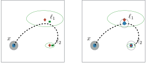
Figure 1: Example: robot with a reachability objective. The red diamonds are the means of the landmarks’ pose distributions and the ellipsoids are the associated $95\%$-confidence regions. The robot is represented by the blue dot. The green squares represent the true locations of landmarks $l_{1}$ and $l_{2}$.

In the case of a safety constraint, e.g., $\varphi_{safe}=\square p$ where $p:=d(x,l_{i}^{p})>1$ for any landmark $i$, once the robot gets close to $l_{1}$ the $\delta$-probably correct product system will transition to the non-accepting sink because there exists a sample map $m$ such that the safety constraint is violated. Thus, in any run that is safe in $\mathcal{G}^{\delta}$, the robot is able to safely avoid both $l_{1}$ and $l_{2}$ with probability $\delta$.

IV Reduction to Deterministic Shortest Path

For a fixed confidence $\delta$, due to Thm. 1, we can convert Problem 1 to a deterministic shortest path problem within the probably correct product system $\mathcal{G}^{\delta}$. In this case, $\mathbb{P}(q_{\tau+1}\notin F)\in\{0,1\}$ and the optimal solution to Problem 1 is either to stop immediately ($\tau=0$), incurring cost $\kappa$, or to find a robot trajectory satisfying $\varphi$ with cumulative motion cost less than $\kappa\delta$. The latter corresponds to the following deterministic problem.

Problem 2.

Given an initial robot state $x_{0}\in X$, a semantic map distribution $\mathcal{P}$, a confidence $\delta\in(0,1)$, and an LTL co-safe formula $\varphi$ represented by a DFA $\mathcal{A}_{\varphi}$, choose a stopping time $\tau$ and a sequence of control inputs $u_{t}\in U$ for $t=0,1,\ldots$ that minimize the motion cost of a trajectory that satisfies $\varphi$:

$$\min_{u_{0},u_{1},\ldots,u_{\tau}}\; \sum_{t=0}^{\tau}c(x_{t},x_{t+1})$$

s.t. $$x_{t+1}=f(x_{t},u_{t}),$$

$$q_{t+1}=T(q_{t},L^{\delta}(x_{t},\mathcal{P})),\;\forall 0\leq t<\tau,$$

$$q_{\tau+1}\in F,$$

$$\sum_{t=0}^{\tau}c(x_{t},x_{t+1})\leq\kappa\delta.$$

If Problem 2 is infeasible, it is best in Problem 1 to stop immediately ($\tau=0$), incurring cost $\kappa$; otherwise, the robot should follow the control sequence $u^{*}_{0:\tau}$ computed above and the corresponding trajectory $x^{*}_{0:\tau+1}$ to incur cost:

$$\sum_{t=0}^{\tau}c(x_{t}^{*},x^{*}_{t+1})+\kappa(1-\delta)\leq\kappa$$

in the original Problem 1. Since Problem 2 is a deterministic shortest path problem, we can use any of the traditional motion planning algorithms, such as RRT [20], RRT* [14, 13] or A* [21] to solve it. We choose A* due to its completeness guarantees [26] and because the automaton $\mathcal{A}_{\varphi}$ can be used to guide the search as we show next.

IV-A Admissible Heuristic

The efficiency of A* can be increased dramatically by designing an appropriate heuristic function to guide the search. Given a state $s:=(x,q)$ in the product system (Def. 3), a heuristic function $h:S\rightarrow\mathbb{R}$ provides an estimate of the optimal cost $h^{*}(s)$ from $s$ to the goal set $S_{F}$. If the heuristic function is admissible, i.e., never overestimates the cost-to-go ($h(s)\leq h^{*}(s),\;\forall s\in S$), then A* is optimal [26].

Lacerda et al. [18] propose a distance metric to evaluate the progression of an automaton state with respect to an LTL co-safe formula. We use a similar idea to design an admissible heuristic function. We partition the state space $Q$ of $\mathcal{A}_{\varphi}$ into level sets as follows. Let $Q_{0}:=F$ and for $i\geq 0$ construct $Q_{i+1}:=\{q\in Q\setminus\bigcup_{k=0}^{i}Q_{k}\mid\exists q^{\prime}\in Q_{i},a\in 2^{\mathcal{AP}},\text{ such that }T(q,a)=q^{\prime}\}$. The generation of level sets stops when $Q_{i}=\emptyset$ for some $i$. Further, we denote the set of all sink states by $Q_{\infty}$. Thus, given $q\in Q$ one can find a unique level set $Q_{i}$ such that $q\in Q_{i}$. We say that $i$ is the level of $q$ and denote it by $\mathsf{Level}(q)=i$.

Proposition 2.

Let $s_{0:t}$ be a trajectory of the product system $\mathcal{G}^{\delta}$ that reaches $S_{F}$, i.e., $s_{t}\in S_{F}$. Then, for any $0\leq k<t$, given $s_{k}=(x_{k},q_{k})$ and $s_{k+1}=(x_{k+1},q_{k+1})$, it holds that $\mathsf{Level}(q_{k})\leq\mathsf{Level}(q_{k+1})+1$.

Proof.

Since $T(q_{k},L^{\delta}(x_{k+1},\mathcal{P}))=q_{k+1}$, if $q_{k+1}\in Q_{i}$ for some level $i$, then, by construction of the level sets, either $q_{k}\in Q_{i+1}$ or $q_{k}\in\bigcup_{j=0}^{i}Q_{j}$. ∎

By construction of the level sets, the automaton states $q_{0:t}$, associated with any trajectory $s_{0:t}$ of the product system that reaches a goal state ($s_{t}\in S_{F}$), have to pass through the level sets sequentially. In other words, if $\mathsf{Level}(q_{0})=i$, then there exists a subsequence $q^{\prime}_{0:i}$ of $q_{0:t}$ such that $\mathsf{Level}(q^{\prime}_{1})=i-1$, $\mathsf{Level}(q^{\prime}_{2})=i-2,\ldots,\mathsf{Level}(q^{\prime}_{i})=0$. Thus, we can construct a heuristic function that underestimates the cost-to-go from some state $s:=(x,q)\in S$ with $\mathsf{Level}(q)=i$ by computing the minimum cost to to reach a state $s^{\prime}:=(x^{\prime},q^{\prime})$ such that $\mathsf{Level}(q^{\prime})\in\{i-1,i\}$ and $q\neq q^{\prime}$. To do so, we determine all the labels that trigger a transition from $q$ to $q^{\prime}$ in $\mathcal{A}_{\varphi}$ and then find all the robot states $\mathcal{B}$ that produce those labels. Then, $h(x,q)$ is the minimum distance from $x$ to the set $\mathcal{B}$. The details of this construction and other functions needed for A* search with LTL specifications, are summarized in Alg. 2.

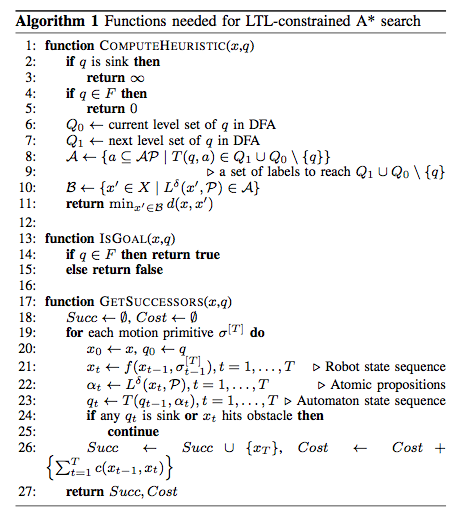
Figure 2: Functions needed for LTL-constrained A* search

Proposition 3.

The heuristic function in Alg. 2 is admissible.

Proof.

See Appendix A-D. ∎

Prop. 3 guarantees that A* will either find the optimal solution to Problem 2 or will report that Problem 2 is infeasible. In the latter case, the robot cannot satisfy the logic specification with confidence $\delta$ and it should either reduce $\delta$ or stop planning.

Note that while the heuristic function is admissible, it is not guaranteed that it is also consistent. Consider two arbitrary states $(x,q)$ and $(x^{\prime},q^{\prime})$ with $\mathsf{Level}(q)=n$ and $\mathsf{Level}(q^{\prime})=n+1$. It is possible that the cost to get from $(x,q)$ to a place in the environment, where a transition to level $n-1$ occurs, is very large, i.e., $h(x,q)$ is large, but it might be very cheap to get from $(x^{\prime},q^{\prime})$ to $(x,q)$ and vice versa. In other words, it is possible that the following inequalities hold:

$$c(x,x^{\prime})+h(x^{\prime},q^{\prime})\leq c(x,x^{\prime})+c(x^{\prime},x)<h(x,q),$$

which makes the heuristic in Alg. 2 inconsistent. We emphasize that, even with an inconsistent heuristic, $A^{*}$ can be very efficient if a technique such as bi-directional pathmax is employed to propagate heuristics between neighboring states [32].

IV-B Accelerating A* Search using Motion Primitives

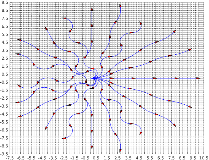
Figure 3: The set of motion primitives used for LTL-constrained A* planning. Each segment contains 5 robot poses indicated by the red triangles. Each robot pose represents a different motion primitive.

If willing to sacrifice completeness, one can significantly accelerate the A* search by using motion primitives for the robot in order to construct a lattice-based graph [28]. The advantage of such a construction is that the underlying graph is sparse and composed of dynamically-feasible robot trajectories that can incorporate a variety of constraints. We present motion primitives for a differential-drive robot in Fig. 3 but much more general models can be handled [6].

A motion primitive is similar to the notion of macro-action [8, 5] and consists of a collection of control inputs $\sigma^{[T]}:=(u_{0},u_{2},\ldots,u_{T-1})$ that are applied sequentially to a robot state $x_{t}$ so that:

$$x_{t+1+k}=f(x_{t+k},\sigma^{[T]}(k)),\;k=0,\ldots,T-1.$$

Instead of using the original control set $U$, we can plan with a set $\bar{U}:=\{\sigma^{[T_{j}]}_{j}\}$ of motion primitives (see GetSuccessors in Alg. 2). In our experiments, the motion primitives were designed offline. Twenty locations with outward facing orientations were chosen on the perimeter of a circle of radius 10 m. A differential-drive controller was used to to generate a control sequence of length $5$ that would lead a robot at the origin to each of the selected locations. Fig. 3 shows the resulting set of motion primitives. They are wavy because the controller tries to follow a straight line using a discrete set of velocity and angular-velocity inputs.

Summary. We formulate the temporal logic planning with a semantic map distribution as a stochastic optimal control problem (Problem 1). Since Problem 1 is intractable, we reduce it to a deterministic shortest path problem (Problem 2) with probabilistic correctness guaranteed by Thm 1. We can solve Problem 2 optimally using A* because the heuristic function proposed in Alg. 2 is admissible (Prop. 3). The obtained solution is partial with respect to Problem 1 because, rather than a controller that trades off the probability of satisfying the specification and the total motion cost, it provides the optimal controller in a subspace of deterministic controllers that guarantee that the probability of satisfying the specification is $\delta$.

V Examples

In this section, we demonstrate the method for LTL-constrained motion planning with a differential-drive robot with state $\mathsf{x}_{t}:=(x_{t},y_{t},\theta_{t})^{T}\in SE(2)$, where $(x_{t},y_{t})$ and $\theta_{t}$ are the 2D position and orientation of the robot, respectively. The kinematics of the robot are discretized using a sampling period $\tau$ as follows:

$$\begin{pmatrix}x_{t+1}\\ y_{t+1}\\ \theta_{t+1}\end{pmatrix}\!=\!\begin{pmatrix}x_{t}\\ y_{t}\\ \theta_{t}\end{pmatrix}+\begin{cases}\begin{pmatrix}\tau\nu\cos(\theta_{t}+\tau\omega/2)\\ \tau\nu\sin(\theta_{t}+\tau\omega/2)\\ \tau\omega\end{pmatrix},\;\lvert\tau\omega\rvert<0.001,\\ \begin{pmatrix}\frac{\nu}{\omega}(\sin(\theta_{t}+\tau\omega)-\sin\theta_{t})\\ \frac{\nu}{\omega}(\cos\theta_{t})-\cos(\theta_{t}+\tau\omega))\\ \tau\omega\end{pmatrix},\;\textrm{else.}\end{cases}$$

The mobile robot is controlled by motion primitives in Fig. 3, whose segments are specified by $\nu=1\;m/\textrm{s}$, $\tau=2\;\textrm{s}$, and $\omega\in[-3,3]\;\textrm{rad}/\textrm{s}$.

The LTL constraints were specified over the two types of atomic propositions for object classes $\mathcal{C}=\{\mathsf{Sq},\mathsf{Cir},\mathsf{Hex},\mathsf{Dia},\mathsf{Tri}\}$. Proposition $\alpha_{i}^{c}(h)$ means the class of $i$-th landmark is $h$ for $h\in\mathcal{C}$. Proposition $\alpha_{i}^{p}(r):\;d(x^{p}-l_{i}^{p})\leq r$ means the robot is $r$-close to landmark $l_{i}$.

The following LTL specification was given to the robot:

$$\varphi:\;(\lozenge(\phi_{1}\land\lozenge(\phi_{2}\land\lozenge\phi_{3}))\land\lozenge\phi_{4})\land\square\phi_{safe}$$

where $\phi_{i}$, $i=1,\ldots,4$ are the following propositional logic formulas:

$$\phi_{1}: =\alpha_{i}^{p}(1)\land\alpha_{i}^{c}(\mathsf{Tri}), i \in\{1,\ldots,M\}$$

$$\phi_{2}: =\alpha_{i}^{p}(2)\land\alpha_{i}^{c}(\mathsf{Dia})\land\alpha_{j}^{p}(2)\land\alpha_{j}^{c}(\mathsf{Cir}), i,j \in\{1,\ldots,M\}$$

$$\phi_{3}: =\alpha_{i}^{p}(2)\land\alpha_{i}^{c}(\mathsf{Sq})\land\alpha_{j}^{p}(2)\land\alpha_{j}^{c}(\mathsf{Cir}), i,j \in\{1,\ldots,M\}$$

$$\phi_{4}: =\alpha_{i}^{p}(1)\land\alpha_{i}^{c}(\mathsf{Hex}), i \in\{1,\ldots,M\}$$

and for $i,j\in\{1,\ldots,M\}$ the safety constraint is:

$$\phi_{safe}:=\square\neg(\alpha_{i}^{p}(2)\land\alpha_{i}^{c}(\mathsf{Sq})\land\alpha_{j}^{p}(2)\land\alpha_{j}^{c}(\mathsf{Sq})).$$

In other words, the robot needs to first visit a triangle, then go to a region where it is close to both a circle and a diamond, and finally visit a region where it is close to both a circle and a square, while visiting a hexagon at some point and avoiding getting stuck between any two squares.

Several case studies were carried out using a simulated semantic map distribution. Robot trajectories with least cost that satisfy the LTL specification with confidence $\delta=0.95$ for different initial conditions were computed with A* and are shown in Fig. 4. Optimal paths with the same initial conditions but different confidence parameters $\delta=0.95$ and $0.5$ are shown in Fig. 5. As expected, we observe a trade-off between the probability of satisfying the LTL formula and the total cost of the path. With a lower confidence ($\delta=0.5$), the total cost for satisfying the LTL formula is also lower than that of a path which satisfies the formula with a high confidence ($\delta=0.95$). Particularly, the uncertainty in the pose of triangle $l_{1}$ with pose distribution $\bar{l}_{1}^{p}=(2.5,1.19)$ is the main reason for the difference in the planned trajectories. With $\delta=0.95$, even though the robot can reach the vicinity of triangle $l_{1}$, it does not have enough confidence to ensure that the triangle would be visited. Instead, it plans to visit another triangle $l_{2}$ for which the uncertainty in the pose distribution $\bar{l}_{2}^{p}=(-5.18,12.04)$ is smaller. Reducing the confidence requirements allows the robot to plan a path that visits triangle $l_{1}$ and has a lower total cost compared to that of visiting triangle $\l_{2}$.

VI Conclusion

This paper proposes an approach for planning optimal robot trajectories that probabilistically satisfy temporal logic specifications in uncertain semantic environments. By introducing a $\delta$-confident labeling function, we show that the original stochastic optimal control problem in the continuous space of semantic map distributions can be reduced to a deterministic optimal control problem in the $\delta$-confidence region of the map distribution. Guided by the automaton representation of the LTL co-safe specification, we develop an admissible A* algorithm to solve the deterministic problem. The advantage of our approach is that the deterministic problem can be solved very efficiently and yet the planned robot trajectory is guaranteed to have minimum cost and to satisfy the logic specification with probability $\delta$.

This work takes an initial step towards integration of semantic SLAM and motion planning under temporal logic constraints. In future work, we plan to extend this method to handle the following: 1) landmark class uncertainty, 2) robot motion uncertainty, 3) a more general class of LTL specifications, 4) map distributions that are changing online. Our goal is to develop a coherent approach for planning autonomous robot behaviors that accomplish high-level temporal logic tasks in uncertain semantic environments.

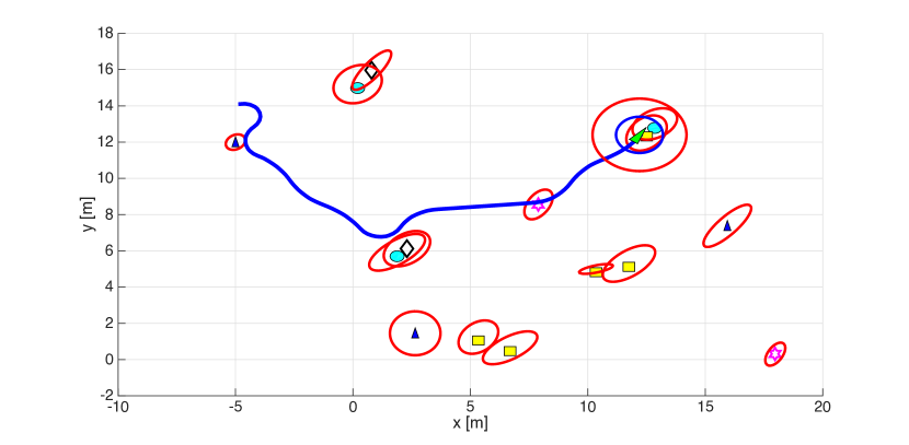
(a) $x_{0}=[-5,14,\pi/6]^{T}$, total motion cost $24\;m$.

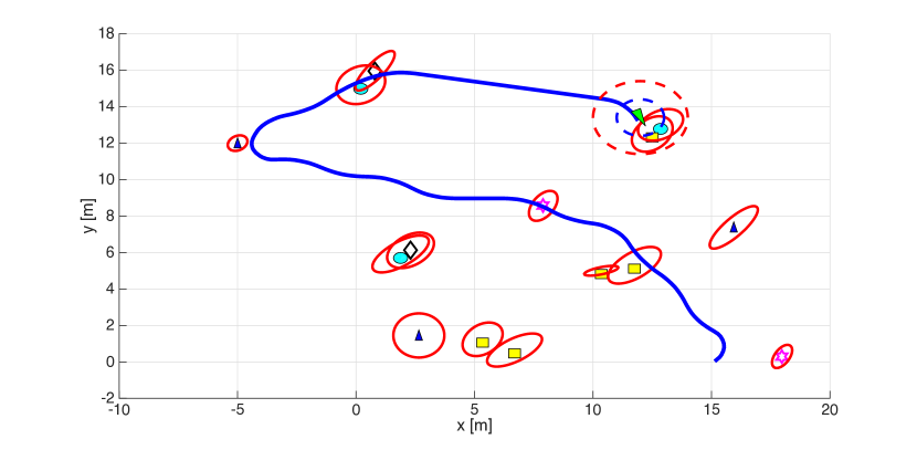
(b) $x_{0}=[15,0,\pi/6]^{T}$, total motion cost $44\;m$.

Figure 4: Robot trajectories obtained by the planning algorithm with different initial conditions. The green triangle represents the mobile robot. The blue dash circle indicates the unit ball and the red dash circle indicates a ball of radius $2\;m$. The red sold ellipses represent the $0.95$-confidence region of the landmark pose distributions. The landmark coordinates are drawn according to the mean of the pose distribution.

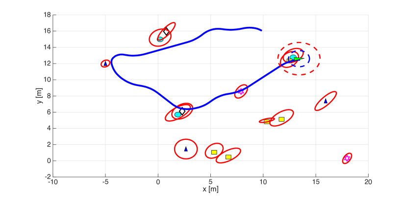
(a) The optimal plan with $0.95$-confidence and motion cost $38\;m$.

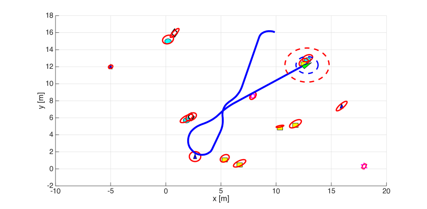
(b) The optimal plan with $0.5$-confidence and motion cost $34\;m$.

Figure 5: Robot trajectories obtained by the planning algorithm with different confidence parameters. The initial state is $x_{0}=[10,16,0.77\pi]^{T}$.

Appendix A Appendix

A-A Proof of Prop. 1

Let $x_{k}$ be the state at time $k$. If for all samples $m$ in the $\delta$-confidence region of $\mathcal{P}$, $L(x_{k},m)=L(x_{k},\bar{\mathcal{M}})$, then $L^{\delta}(x_{k},\mathcal{P})=L(x_{k},\bar{\mathcal{M}})$, which equals $L(x_{k},\mathcal{M})$ with probability $\delta$. Otherwise, $L^{\delta}(x_{k},\mathcal{P})=\lambda$ (empty string). Since $k$ is arbitrary, we can conclude that $L^{\delta}(x_{0:t},\mathcal{P})$ is a subsequence of $L(x_{0:t},\mathcal{M})$ with probability $\delta$. ∎

A-B Proof of Thm. 1

Since the language $\mathcal{L}(\mathcal{A}_{\varphi})$ is a simple polynomial, the following upward closure [27] property holds: For any word $uv\in\mathcal{L}(\mathcal{A}_{\varphi})$ and any $a\in 2^{\mathcal{AP}}$, it holds that $uav\in\mathcal{L}(\mathcal{A}_{\varphi})$. In other words, if any empty string in a word from a simple polynomial language is replaced by a symbol in the alphabet, then the resulting word is still in the language.

For a given robot trajectory $x_{0:\tau}$, let $L^{\delta}(x_{0:\tau},\mathcal{P})=b_{0}b_{1}\ldots b_{\tau}\in\mathcal{L}(\mathcal{A}_{\varphi})$ be the $\delta$-confident label sequence and $L(x_{0:\tau},\mathcal{M})=a_{0}a_{1}\ldots a_{\tau}$ be the true label sequence. According to Prop. 1, for each $0\leq i\leq\tau$, either $a_{i}=b_{i}$ or $a_{i}\neq b_{i}$ and $b_{i}=\emptyset$. Thus, if $b_{0}b_{1}\ldots b_{\tau}$ belongs to $\mathcal{L}(\mathcal{A}_{\varphi})$, $a_{0}a_{1}\ldots a_{\tau}$ must be in $\mathcal{L}(\mathcal{A}_{\varphi})$ because it is obtained by replacing each empty string in $b_{0}b_{1}\ldots b_{\tau}$ with some symbol in $2^{\mathcal{AP}}$ and the language $\mathcal{L}(\mathcal{A}_{\varphi})$ is upward closed.∎

A-C Characterization of LTL co-safe formulas that translate to simple polynomials

Formally, the subset of LTL formulas is defined by the grammar

$$\varphi:=\varphi_{reach}\mid\varphi_{seq}\mid\varphi\land\varphi\mid\varphi\lor\varphi,$$ (3)

where $\varphi_{reach}=\lozenge\phi\mid\varphi_{reach}\land\varphi_{reach}\mid\varphi_{reach}\lor\varphi_{reach}$ represents the reachability, $\varphi_{seq}:=\phi\mid\lozenge\varphi_{seq}\mid\lozenge(\varphi_{seq}\land\lozenge\varphi_{seq})$ is a set of formulas describing sequencing constraints. Here, $\phi$ is a propositional logic formula.

A-D Proof of Prop. 3

We proceed by induction on the levels in $\mathcal{A}_{\varphi}$. In the base case, $q\in Q_{0}\equiv F$ and $h(x,q)=0$ for any $x\in X$. Suppose that the proposition is true for level $n$ and let $(x,q)$ be some state with $x\in X$ and $\mathsf{Level}(q)=n+1$. As before, let $h^{*}(x,q)$ be the optimal cost-to-go. Due to Prop. 2, there are only three possibilities for the next state $(x^{\prime},q^{\prime})$ along the optimal path starting from $(x,q)$:

• $\mathsf{Level}(q^{\prime})=n$: By construction of $h$:

  $$h^{*}(x,q)=c(x,x^{\prime})+h^{*}(x^{\prime},q^{\prime})\geq h(x,q)+0.$$

• $\mathsf{Level}(q^{\prime})=n+1$: Same conclusion as above.

• $\mathsf{Level}(q^{\prime})=k>n+1$: In this case, there exists another state $(x^{\prime\prime},q^{\prime\prime})$ later along the optimal path such that $\mathsf{Level}(q^{\prime\prime})=n+1$ (otherwise the optimal path cannot reach the goal set). Then, by the triangle inequality for the motion cost $c$:

  $$h^{*}(x,q) =c(x,x^{\prime})+c(x^{\prime},x^{\prime\prime})+h^{*}(x^{\prime\prime},q^{\prime\prime})$$

  $$\geq c(x,x^{\prime\prime})+0\geq h(x,q)$$

Thus, we conclude that $h^{*}(x,q)\geq h(x,q)\geq 0$ for all $x\in X$ and $q\in Q$. ∎

References

- Atanasov et al. [2014] N. Atanasov, M. Zhu, K. Daniilidis, and G. Pappas. Semantic Localization Via the Matrix Permanent. In Robotics: Science and Systems, 2014.
- Bachrach et al. [2012] A. Bachrach, S. Prentice, R. He, P. Henry, A. S. Huang, M. Krainin, D. Maturana, D. Fox, and N. Roy. Estimation, planning, and mapping for autonomous flight using an rgb-d camera in GPS-denied environments. The International Journal of Robotics Research, 31(11):1320–1343, 2012.
- Bao and Savarese [2011] S. Bao and S. Savarese. Semantic Structure from Motion. In IEEE Conf. on Computer Vision and Pattern Recognition (CVPR), pages 2025–2032, 2011.
- Bhatia et al. [2010] A. Bhatia, L. E. Kavraki, and M. Y. Vardi. Sampling-based motion planning with temporal goals. In IEEE International Conference on Robotics and Automation, pages 2689–2696. IEEE, 2010.
- Botea et al. [2005] A. Botea, M. Enzenberger, M. Muller, and J. Schaeffer. Macro-FF: Improving AI planning with automatically learned macro-operators. Journal of Artificial Intelligence Research, 24:581–621, 2005.
- Cohen et al. [2011] B. Cohen, G. Subramanian, S. Chitta, and M. Likhachev. Planning for Manipulation with Adaptive Motion Primitives. In IEEE International Conference on Robotics and Automation, pages 5478–5485, 2011.
- Ding et al. [2014] X. Ding, S. Smith, C. Belta, and D. Rus. Optimal control of Markov decision processes with linear temporal logic constraints. IEEE Transactions on Automatic Control, 59(5):1244–1257, May 2014.
- Fikes and Nilsson [1971] R. Fikes and N. Nilsson. Strips: A new approach to the application of theorem proving to problem solving. Artificial Intelligence, 2(3):189–208, 1971.
- Fu and Topcu [2014] J. Fu and U. Topcu. Probably approximately correct mdp learning and control with temporal logic constraints. In Proceedings of Robotics: Science and Systems, Berkeley, USA, July 2014.
- Guez and Pineau [2010] A. Guez and J. Pineau. Multi-tasking SLAM. In IEEE International Conference on Robotics and Automation, pages 377–384, 2010.
- Guo et al. [2013] M. Guo, K. H. Johansson, and D. V. Dimarogonas. Revising motion planning under linear temporal logic specifications in partially known workspaces. In IEEE International Conference on Robotics and Automation, pages 5025–5032, 2013.
- Johnson and Kress-Gazit [2015] B. Johnson and H. Kress-Gazit. Analyzing and revising synthesized controllers for robots with sensing and actuation errors. The International Journal of Robotics Research, 34(6):816–832, 2015.
- Karaman and Frazzoli [2012] S. Karaman and E. Frazzoli. Sampling-based algorithms for optimal motion planning with deterministic -calculus specifications. In American Control Conference, pages 735–742, 2012.
- Karaman and Frazzoli [2011] S. Karaman and E. Frazzoli. Sampling-based algorithms for optimal motion planning. The International Journal of Robotics Research, 30(7):846–894, 2011.
- Kloetzer and Belta [2008] M. Kloetzer and C. Belta. A fully automated framework for control of linear systems from temporal logic specifications. IEEE Transactions on Automatic Control, 53(1):287–297, 2008.
- Kress-Gazit et al. [2009] H. Kress-Gazit, G. E. Fainekos, and G. J. Pappas. Temporal-logic-based reactive mission and motion planning. IEEE Transactions on Robotics, 25(6):1370–1381, 2009.
- Kupferman and Vardi [2001] O. Kupferman and M. Y. Vardi. Model checking of safety properties. Formal Methods in System Design, 19(3):291–314, 2001.
- Lacerda et al. [2015] B. Lacerda, D. Parker, and N. Hawes. Optimal policy generation for partially satisfiable co-safe LTL specifications. In International Joint Conference on Artificial Intelligence, pages 1587–1593, 2015.
- Lahijanian et al. [2010] M. Lahijanian, J. Wasniewski, S. B. Andersson, and C. Belta. Motion planning and control from temporal logic specifications with probabilistic satisfaction guarantees. In Robotics and Automation (ICRA), 2010 IEEE International Conference on, pages 3227–3232. IEEE, 2010.
- LaValle [1998] S. LaValle. Rapidly-Exploring Random Trees A New Tool for Path Planning. Technical Report Computer Science Dept., TR 98-11, Iowa State University, 1998.
- Likhachev et al. [2004] M. Likhachev, G. Gordon, and S. Thrun. ARA* : Anytime A* with Provable Bounds on Sub-Optimality. In Advances in Neural Information Processing Systems, pages 767–774. 2004.
- Livingston et al. [2012] S. C. Livingston, R. M. Murray, and J. W. Burdick. Backtracking temporal logic synthesis for uncertain environments. In IEEE International Conference on Robotics and Automation, pages 5163–5170, 2012.
- Livingston et al. [2013] S. C. Livingston, P. Prabhakar, A. B. Jose, and R. M. Murray. Patching task-level robot controllers based on a local -calculus formula. In IEEE International Conference on Robotics and Automation, pages 4588–4595, 2013.
- Missiuro and Roy [2006] P. E. Missiuro and N. Roy. Adapting probabilistic roadmaps to handle uncertain maps. In IEEE International Conference on Robotics and Automation, pages 1261–1267, 2006.
- Nüchter and Hertzberg [2008] A. Nüchter and J. Hertzberg. Towards Semantic Maps for Mobile Robots. Robotics and Autonomous Systems, 56(11):915–926, 2008.
- Pearl [1984] J. Pearl. Heuristics: Intelligent Search Strategies for Computer Problem Solving. Addison-Wesley, 1984.
- Pin [2010] J.-É. Pin. Mathematical foundations of automata theory. Lecture notes LIAFA, Université Paris, 7, 2010.
- Pivtoraiko and Kelly [2005] M. Pivtoraiko and A. Kelly. Generating near minimal spanning control sets for constrained motion planning in discrete state spaces. In IEEE/RSJ International Conference on Intelligent Robots and Systems, pages 3231–3237, 2005.
- Pnueli [1981] A. Pnueli. The temporal semantics of concurrent programs. Theoretical Computer Science, 13(1):45 – 60, 1981.
- Salas-Moreno et al. [2013] R. Salas-Moreno, R. Newcombe, H. Strasdat, P. Kelly, and A. Davison. SLAM++: Simultaneous Localisation and Mapping at the Level of Objects. In IEEE Conf. on Computer Vision and Pattern Recognition (CVPR), pages 1352–1359, 2013.
- Wolff et al. [2012] E. M. Wolff, U. Topcu, and R. M. Murray. Robust control of uncertain markov decision processes with temporal logic specifications. In IEEE Annual Conference on Decision and Control, pages 3372–3379, 2012.
- Zhang et al. [2009] Z. Zhang, N. Sturtevant, R. Holte, J. Schaeffer, and A. Felner. A* search with inconsistent heuristics. In International Joint Conference on Artificial Intelligence, pages 634–639, 2009.