Accurate theoretical prediction on positron lifetime of bulk materials

Abstract

Based on the first-principles calculations, we perform an initiatory statistical assessment on the reliability level of theoretical positron lifetime of bulk material. We found the original generalized gradient approximation (GGA) form of the enhancement factor and correlation potentials overestimates the effect of the gradient factor. Furthermore, an excellent agreement between model and data with the difference being the noise level of the data is found in this work. In addition, we suggest a new GGA form of the correlation scheme which gives the best performance. This work demonstrates that a brand-new reliability level is achieved for the theoretical prediction on positron lifetime of bulk material and the accuracy of the best theoretical scheme can be independent on the type of materials.

I Introduction

During recent years positron annihilation spectroscopy (PAS) has become a valuable method to study the microscopic structure of solids [1, 2] and gives detailed information on the electron density and momentum distribution [3, 4, 5] in the regions scanned by positrons. For a thorough understanding and interpretation of experimental results, an accurate theory is needed. Exact many-body theory calculations on annihilation rate and scattering dynamics can be implemented for the positron in small atom or molecule system [6, 7, 8], but is time-consuming for the positron in large many-electron system. Based on the density functional theory (DFT) [9], a full two-component self-consistent scheme [10, 11] has been developed for calculating positron states in solids. Especially in bulk material where the positron is delocalized and does not affect the electron states, the full two-component scheme can be reduced without losing accuracy to the conventional scheme [10, 11] in which the electronic-structure is determined by usual one-component formalism. However, there are various kinds of approximations on electron-positron correlation can be adjusted within this calculations. To improve the analyses of experimental data [12, 13], we should find out which approximations are more credible to predict the positron lifetimes. Thus, in this short paper, we focus on probing the reliability level of these approximations for calculating the positron lifetimes in bulk materials.

Recently, Drummond et al. [14] made the most accurate calculations for a positron in a homogeneous electron gas by using Quantum Monte Carlo (QMC) method and gave a smaller enhancement factor compared with the popular expression [15]. Very recently, Kuriplach and Barbiellini [16, 17] implemented multiple calculations of positron-annihilation characteristics in solid based on the local density approximation (LDA) or generalized gradient approximation (GGA) forms of the enhancement factor and correlation potential provided by the perturbed hypernetted chain (PHC) calculation [18, 19] or reparameterized from Drummond et al.’s QMC results. Their results showed that the recent two GGA forms of the correlation schemes are needed to improve the calculated positron lifetimes. But it’s hard to clearly judge and distinguish the reliability level of these two GGA models based on one by one comparisons with a small number of materials. For more recent studies on the calculations of positron lifetimes, see Refs. [19, 20].

In this paper, we investigate nine LDA/GGA correlation schemes containing a new GGA form for positron lifetime calculations based on the full-potential linearized augmented plane-wave (FLAPW) plus local orbitals approach [21] for accurate electronic-structure calculations. The experimental data used in this work are composed of many observed values of materials more than twice as much as previous works [16, 17, 19, 20]. To take into account the fact that the materials having more credible experimental values should play more important roles in these assessments, the measurement errors of these experimental values are assumed being Gaussian and then estimated by the standard deviations of collected observed values from different literatures and/or groups as in Ref. [22]. Furthermore, five subsets are structured depending on the number of observed values of each material to make a subtler probe. By utilizing this data, we do the initiatory numerical and statistic assessment on the reliability level of various LDA and/or GGA correlation schemes for positron lifetime calculations.

This paper is organized as follows: In Sec. II, we give a brief description of the models considered here as well as the analysis methods we used. In Sec. III, we introduce the experimental data on positron lifetime used in this work. In Sec. IV, we give the results and make some discussion based on the visualized and statistic analyses. In Sec. V, we make some conclusions of this work. In addition, we present a appendix with a table listing all calculated theoretical lifetimes.

II Theory and methodology

II.1 Theory

The positron lifetime which is the inverse of positron annihilation rate can be obtained by the following equations [15] in bulk materials,

$$\tau_{e+}=\frac{1}{\lambda},\ \ \lambda=\pi r_{0}^{2}c\int d\vec{r}n_{e-}(\vec{r})n_{e+}(\vec{r})\gamma(n_{e-}),$$ (1)

where $r_{0}$ is the classical electron radius, $c$ is the speed of light, and $\gamma(n_{e-})$ is the enhancement factor arising from the contact pair-correlation between positron and electrons. For a perfect lattice, the conventional scheme is still accurate as in this case the positron density is delocalized and vanishingly small at every point thus does not affect the bulk electronic-structure [11, 15]. So in this paper the electronic density $n_{e-}(\vec{r})$ were calculated without considering the perturbation by positron based on the FLAPW approach [21] which is regarded as the most accurate method for electronic-structure calculations. The total potential sensed by positron is composed of the Coulomb potential and the correlation potential [15] between electrons and positron. Then, the positron density can be determined by solving the Kohn-Sham equation [16].

Table 1: Nine parameterized LDA/GGA correlation schemes.

$\gamma$	$a_{2}$	$a_{3}$	$a_{3/2}$	$a_{5/2}$	$a_{7/3}$	$a_{8/3}$	$\alpha$
BNLDA	-1.26	$1/6-1/6\epsilon_{\infty}$	0.8295	0.3286	0	0	0
APLDA	-0.0742	1/6	0	0	0	0	0
APGGA	-0.0742	1/6	0	0	0	0	0.22
PHCLDA	-0.137	1/6	0	0	0	0	0
PHCGGA	-0.137	1/6	0	0	0	0	0.10
QMCLDA	8.6957	0.1737	-3.382	0	-7.37	1.756	0
QMCGGA	8.6957	0.1737	-3.382	0	-7.37	1.756	0.063
fQMCLDA	-0.22	1/6	0	0	0	0	0
fQMCGGA	-0.22	1/6	0	0	0	0	0.05

The forms of enhancement factor and correlation potential can be divided into two categories: the LDA and the GGA. Within the LDA, the corresponding correlation potential $V_{corr}^{\text{LDA}}$ given by Ref. [15] is used. Within the GGA, the corresponding correlation potential takes the form [24, 25] $V_{corr}^{\text{GGA}}=V_{corr}^{\text{LDA}}e^{-\alpha\epsilon/3}$, here $\alpha$ is an experiential parameter, and $\epsilon$ is defined as $\epsilon=|\nabla\ln(n_{e-})|^{2}/q_{\text{TF}}^{2}$, ($q_{\text{TF}}^{-1}$ is the local Thomas-Fermi screening length). We investigated eight existing forms of the enhancement factor and correlation potential marked by BNLDA[23], APLDA[24], APGGA[24, 25], PHCLDA[18],PHCGGA[19], QMCLDA[14], fQMCLDA[16] and fQMCGGA[16], plus a new GGA form QMCGGA. All forms of the enhancement factor can be parameterized by the following equation,

$$\gamma= 1+(1.23r_{s}+a_{2}r_{s}^{2}+a_{3}r_{s}^{3}+a_{3/2}r_{s}^{3/2} +\ a_{5/2}r_{s}^{5/2}+a_{7/3}r_{s}^{7/3}+a_{8/3}r_{s}^{8/3})e^{-\alpha\epsilon},$$ (2)

here $r_{s}$ is defined by $r_{s}=(3/4\pi n_{e-})^{1/3}$, and the values of the parameters $a_{2},a_{3},a_{3/2},a_{5/2},a_{7/3},a_{8/3},\text{and }\alpha$ are listed in Table 1 according to specific kind of the correlation scheme. The QMCGGA form proposed in this work is derived from the original QMCLDA parametrization introduced by Drummond et al. [14], instead of the APLDA parametrization used to fit the QMCLDA results within the fQMCLDA and the fQMCGGA. The adoption of the QMCLDA parametrization is due to the fact that the existence of positive $a_{8/3}$ term and the lager $a_{3}$ term lead to a much lager enhancement in the high $r_{s}$ rigion compared with the fQMCLDA form. Nevertheless, the difference between QMCLDA and fQMCLDA at low $r_{s}$ ($r_{s}<6$) is minor and the fitted parameter $\alpha$ is only slightly changed from 0.05 to 0.063, which will result in similar lifetime values for most materials.

II.2 Computational details

In practice of this work, The WIEN2k code [26] was used for the FLAPW electronic-structure calculations. The PBE-GGA approach [27] was adopted for electron-electron exchange-correlations, the total number of k-points in the whole Brillouin zone (BZ) was set to 3375, the default values of muffin-tin radius were used, and the self-consistency was achieved up to both levels of 0.0001 Ry for total energy and 0.001 e for charge distance. To obtain the positron-state, the three-dimensional Kohn-Sham equation was solved by the finite-difference method while the unit cell of each material was divided into about 10 mesh spaces per $bohr$ in each dimension. All important variable parameters were checked carefully to achieve that the computational precision of lifetime values are at most the order of 0.1 ps.

Table 2: The number of observed values $n_{\textbf{obs}}$, the high-frequency dielectric constant $\epsilon_{\infty}$, the experimental values of lifetime $\tau_{\textbf{exp}}$ alongwith the corresponding mean value ${\tau}_{\textbf{exp}}^{*}$, and the standard deviation $\sigma_{\textbf{exp}}$ for each material in this work. The high-frequency dielectric constants not listed here will be set to $\infty$ as in Ref. [28].

$n_{\textbf{obs}}$	Material	$\epsilon_{\infty}$	$\tau_{\textbf{exp}}$	${\tau}_{\textbf{exp}}^{*}$	$\sigma_{\textbf{exp}}$
1	Li	-	291 [30]	291	-
	Na	-	338[30]	338	-
	K	-	397[30]	397	-
	Rb	-	406[30]	406	-
	Cs	-	418[30]	418	-
	Ga	-	198[31]	198	-
	Cr	-	120 [31]	120	-
	Sc	-	230[32]	230	-
	Y	-	249[31]	249	-
	TiO	-	140 [33]	140	-
	GaN	5.4[23]	180[23]	180	-
	ZnS	5.4[34]	230[34]	230	-
	ZnTe	7.28[34]	266[34]	266	-
	HgTe	15[34]	274[35]	274	-
	ZnSe	5.8[34]	240[34]	240	-
	PbSe	22.9[36]	220[37]	220	-
	NiO	5.7[38]	110[39]	110	-
2	Be	-	137 [31] 142[31]	139.5	3.535
	Pt	-	99[31] 128[31]	113.5	20.51
	Co_alpha	-	118[32] 119[31]	118.5	0.707
	Tl	-	226[31] 229[31]	227.5	2.121
	TiC	-	155[40] 160[41]	157.5	3.535
	SiC_3C	6.52[23]	138[48] 140[42]	139.0	12.02
	GaP	9.1[23]	223[43] 225[44]	224.0	1.414
	InAs	12.3[23]	247[44] 257[45]	252.0	7.071
3	InSb	15.7 [23]	258[23] 280[46] 282[44]	273.3	13.32
	GaSb	14.4 [23]	247[44] 260[23] 260[23]	255.7	7.505
	Bi	-	227.5[31] 238[31] 241[31]	235.5	7.088
	Zr	-	165[47] 163[31] 165[31]	164.3	1.154
	C_diamond	5.66[23]	97.5[31] 107[31] 115[44]	106.5	8.760
	W	-	105[47] 102[31] 116[31]	107.7	7.371
4	Pd	-	96[47] 120[31] 108[31] 118[31]	110.5	11.00
	V	-	120[31] 130[47] 123[31] 130[31]	125.5	5.058
	SiC_6H	6.52[23]	141[48] 140[49] 146[33] 144[33]	142.8	2.753
	MgO	3.0[23]	130[50] 166[33] 152[33] 155[39]	150.8	15.09
5	Si	11.9[31]	216.7[31] 218[31] 218[31] 222[31] 216[31]	218.1	2.323
	Ge	16.0[23]	220.5[31] 230[31] 230[31] 228[31] 228[31]	227.3	3.931
	Mg	-	225[47] 225[31] 220[31] 238[31] 235[31]	228.6	7.569
	Al	-	160.7[31] 166[31] 163[31] 165[31] 165[31]	163.9	2.114
	Ti	-	147[47] 154[31] 145[31] 152[31] 143[31]	148.2	4.658
	Fe	-	108[31] 106[31] 114[31] 110[31] 111[31]	109.8	3.033
	Ni	-	109.8[31] 107[31] 105[31] 109[31] 110[31]	108.2	2.127
	Zn	-	148[47] 153[31] 145[31] 154[31] 152[31]	150.4	3.781
	Cu	-	110.7[31] 122[31] 112[31] 110[31] 120[31]	114.9	2.514
	Nb	-	119[31] 120[31] 122[31] 122[31] 125[31]	121.6	2.302
	Mo	-	109.5[31] 103[31] 118[31] 114[31] 104[31]	109.7	6.418
	Ta	-	116[47] 122[31] 120[31] 125[31] 117[31]	120.0	3.674
	Ag	-	120[31] 130[31] 131[31] 133[32] 131[47]	129.0	5.147
	Au	-	117[31] 113[31] 113[31] 117[31] 123[31]	116.6	4.098
	Cd	-	175[47] 184[31] 167[31] 172[31] 186[31]	176.8	8.043
	In	-	194.7[31] 200[31] 192[31] 193[31] 189[31]	193.7	4.066
	Pb	-	194[47] 200[31] 204[31] 200[31] 209[31]	201.4	5.550
	GaAs	10.9[23]	231.6[51] 231[52] 230[53] 232[54] 220[55]	228.9	5.043
	InP	9.60[23]	241[56] 240[57] 247[23] 242[45] 244[58]	242.8	2.775
	ZnO	3.9[59]	153[60] 159[61] 158[62] 161[63] 171[64]	160.4	6.618
	CdTe	7.2[23]	284[34] 285[65] 285[66] 289[35] 291[44]	286.8	3.033

II.3 Model comparison

To make a comparison between different models, an appropriate criterion must be chosen. The popular one is the root mean squared deviation (RMSD) which is defined as the square root of the mean of the squared deviation between experimental and theoretical results. Beyond this, a comprehensive statistical analysis should be employed where the credibility of observed lifetimes can be estimated by the standard deviations. Therefore, based on the chi-squared analysis, we also adopted $\chi^{2}/dof=\sum^{N}_{i=1}[(X_{i}^{\textbf{exp}}-X_{i}^{\textbf{theo}})^{2}/\sigma_{i}^{2}N]$ as another selection criterion for different models and datasets, where $\sigma_{i}$ is the standard deviation of experimental value for each material, and the $dof$ (degree of freedom) is set to N (the size of corresponding dataset) since the parameters of each model are fixed in this work. In addition, the p-value corresponding to each $\chi^{2}$ is much more meaningful to explore the agreement level of theoretical models and experimental data. From the above definitions, one can see that the experimental data favor models producing lower (higher) values of the RMSD and/or $\chi^{2}/dof$ (p-values). Especially, the models with p-value $<0.01$ are most likely rejected by current collected data.

III Experimental data

We gathered up to five recent observed values from different literatures and/or groups for 56 materials to compose a more reliable experimental dataset which consequently lead to more credible results comparing with previous works [16, 17, 19, 20]. All the data used in this work are listed in Table 2 and collected basically within the standard suggested in Ref. [28]. Older experimental data were avoided being adopted, and only one observed value is used for these materials whose experimental values are all measured before 1975. It’s hard to choose a quantity to estimate their measurement errors. In our previous work [29], only the statistical error of single measurement is used in the model selection criterion. But the deviations of results between different groups are usually much larger than the statistical errors, even when just the recent and reliable measurements are considered. That is, the systematic error is the dominant factor and the sole statistical error is far from enough. However, the systematic error is difficult to derive from single experimental result. The time resolution of related measurement is a correlative quantity but is nearly at the same level in recent years and insufficient, since the quality of material sample is another significant factor which can not be neglected. Unfortunately, the definite effect of sample defect caused by unintentional doping is imponderable. In this paper, instead of focusing on the uncertain error of single experiment, we evaluate the reliability level of average experimental values of each material. As usual, we assume that the distribution of observed values from repeated measurements is Gaussian and the systematic errors tend to be cancelled as expected in Ref. [28], Hence, the measurement uncertainties of related materials can be estimated by the standard deviations of collected observed values from different literatures and/or groups as in Ref. [22]. It is reasonable since the materials with larger scattering observed lifetimes is more debatable and should play less important roles in these assessments. To make a subtle probe, five subsets were structured depending on the number of observed values: (a) subset A includes the overall 56 materials, (b) subset B includes 39 materials having at least two observed values, (c) subset C includes 31 materials having at least three observed values, (d) subset D includes 25 materials having at least four observed values, (e) subset E includes 21 materials having five observed values. It should be noted that, for a more comprehensive assessment including positron lifetimes in defects, the calculations based on the full two-component scheme need to be performed. However, in this work, we focus on testing the calculation methods by using lifetime data of bulk materials because of the insufficient observed values together with their large scattering for vacancy lifetimes and the fact that the conventional scheme is strictly accurate for bulk-lifetime calculations.

IV Results and discussion

IV.1 Visualized analyses

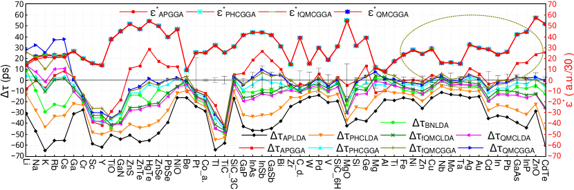
Figure 1: The deviations of the theoretical results based on various approximations from the experimental values $\Delta\tau=\tau_{\text{theo}}-\tau^{*}_{\text{exp}}$ alongwith the standard deviation of experimental values for each material. To make a comparison, the mean electron-density gradient factor $\epsilon^{*}$ sensed by positron for four GGA forms based on the FLAPW calculations are also plotted.

We firstly give visualized comparisons between experimental values and theoretical results based on different correlation schemes. All the detailed numerical theoretical results can be found in appendix. The difference between theoretical results and experimental data along with the standard deviations of observed values for all materials are plotted in Fig. 1. From this figure, the scattering regions of calculated lifetimes by different forms of the enhancement factor are found much larger in the semiconductor systems with bonding states compared with those in pure metal systems excluding the alkali metals. This means the positron lifetimes of semiconductors and alkali metals have more sensitivity to different forms of the enhancement factor. For the GGA approaches, we also plot the average electron-density gradient factor defined by $\epsilon^{*}=\int\epsilon^{e-}_{\text{FLAPW}}\cdot n^{e+}_{\text{GGA}}\cdot d\vec{r}$ in Fig. 1. This figure shows that the four GGA approaches give almost the same values of $\epsilon^{*}$. Furthermore, the most interesting phenomenon in Fig. 1 is that a clear positive correlation between $\epsilon^{*}$ and $\Delta\tau_{\text{APGGA}}$ is found especially in the area of the more credible subset E as marked with olive dashed ellipse. Considering that the presence of electron-density gradient term $\epsilon$ decreases the enhancement factor $\gamma(n_{e-})$ in Eq. (1) and then increases the lifetime, this phenomenon actually indicates that the original GGA form APGGA (with $\alpha=0.22$) overestimates the contribution of the gradient term while for other GGA forms no assured overestimation is appeared.

IV.2 Numerical and statistic analyses

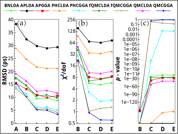
Figure 2: The RMSD (a), $\chi^{2}/dof$ (b) and p-value (b) versus the subsets of data based on different forms of the correlation schemes.

To make a precise and numerical assessment, we plot the values of RMSD for different approaches and subsets of data in Fig. 2(a). Before going on, we mention again that the subsets having more observed values for each material are more credible, that is, the subset E should play the most important role in the following discussions. It is reasonable to see that, with increasing the index of subset from A to E, the RMSDs for most forms of the enhancement factor reach to stable values except three recent GGA forms: PHCGGA, fQMCGGA and QMCGGA. This fact implies that these GGA forms may have the ability to give smaller values of RMSD with more experimental data in the future. Among those forms of enhancement factor based on recent QMC results [14], the fQMCLDA fitted by the Kuriplach and Barbiellini gives a smaller RMSD than the original one QMCLDA while both of them are not good enough. On the contrary, the QMCGGA form proposed in this work performs better than the fQMCGGA form and produces the best RMSD. Therefore, we will focus on discussing QMCGGA and QMCLDA forms instead of the reparameterized forms fQMCLDA and fQMCGGA. Several other phenomena can be found in this figure. Firstly, the QMCLDA form of the enhancement factor makes large progress compared with the older forms APLDA and PHCLDA, and the gradient correction to these LDA forms are still needed to give much better results which is consistent with previous study [16]. Secondly, the phenomenon that the best LDA form (BNLDA) performs a little better than the original GGA form (APGGA) within the exact self-consistent electronic calculation (FLAPW) confirms previous works [20]. There, they claimed that beyond LDA methods are not needed to reach a well level of agreement at that time when accurate band-structure methods (FLAPW) are used. However, our results further show that the recent three GGA approaches (PHCGGA, fQMCGGA and QMCGGA) make significant improvement on the agreement between theoretical and experimental lifetimes compared with the best LDA approach. Finally, based on the FLAPW method, the QMCGGA and PHCGGA forms give a best value of 3.46 ps and a passable value of 5.04 ps for RMSD, respectively. Because the more closer to zero the harder to reduce RMSD, the decrease of RMSD from 5.04 ps to 3.46 ps maybe noteworthy. To investigate this problem, a further statistic analysis is needed for this level of agreement.

To perform a comprehensive analysis taking account of the uncertainty of collected experimental data, a chi-squared analysis has been employed in this work, and the corresponding results of the $\chi^{2}/dof$ and p-value are plotted in Fig. 2(b) and 2(c). These figures give similar but more clear and credible results compared with Fig. 2(a). The most meaningful result is that distinct improvements upon the $\chi^{2}/dof$ and p-value are made by the QMCGGA form compared with the PHCGGA form. Furthermore, the p-values given by the calculations based on the FLAPW method and the QMCGGA approach are 0.55, 0.93 and 0.92 for the subset C, D and E, respectively. The fact that these p-values are larger than 0.05 (related to 95% CL) means that the corresponding deviations between the theoretical values and experimental data can be considered as the noise level of the dataset, so that a brand-new level of agreement is achieved for these materials with the theoretical lifetimes ranging from 104 ps ($\tau_{\textbf{Ni}}$) to 287 ps ($\tau_{\textbf{CdTe}}$). In other words, the calculations based on the FLAPW together with the new QMCGGA are adequately credible for predicting exact positron lifetimes for bulk materials even confronting them with repeated measurements.

Caused by the boosted confidence and that the best scheme (FLAPW & QMCGGA) gives $\text{RMSD}_{min}=3.5$ ps, it is reasonable to conclude that the accuracy of these experimental values with a deviation from the best theoretical value being larger than 10 ps ($\approx 3\times\text{RMSD}_{min}$) should be questioned. As a consequence, the experimental data of the following materials: Cr (120 ps), Sc (230 ps), Y (249 ps), TiO (140 ps), GaN (180 ps), Pt (113.5 ps), Co_alpha (118.5 ps), Tl (227.5 ps), TiC (157.5 ps) and MgO (150.75 ps) should be strongly doubted and their corresponding calculated theoretical values are much more reliable.

But for materials with lower electron densities and larger lifetimes ($\gtrsim 300$ ps), the effectiveness of the best scheme is not proved. From left part of Fig. 1, it is clear that the theoretical lifetimes for alkali-metal given by APGGA and PHCGGA approaches are in much better agreement with current experimental values. So, as shown in Fig. 2(a), the RMSD of QMCGGA related to the dataset A is not better than that of APGGA and PHCGGA. Meanwhile, taking into account the overestimation of the gradient correlation by APGGA prominently for semiconductors with larger $\epsilon^{\star}$, the less semiconductors a dataset involves, the better the APGGA behaves. This is consistent with our previous work where a limited dataset composed of 16 materials including alkali-metals and only three semiconductors is used [29]. There, although the GGA form based on recent QMC simulation performs better for semiconductors, no remarkable improvement for the whole dataset is found. When we take into consideration that the measured values for alkali-metals reported in 1967 are not suggested to be treated seriously [16], the benefit of the two QMC-GGA forms is swamped due to the mixture of reliable data and insufficient data. In addition, the positron density is able to exceed the electron density in the case of positron binding atoms and ions. Significantly, the almost exact annihilation rate calculated using many-body theory method for this atomic-type system [6, 7, 8] allows us to further validate these positron-electron correlation schemes. As mentioned above, the QMCLDA form gives a much larger enhancement factor in the high $r_{s}$ region compared with the reparameterized fQMCLDA form, although their discrepancy at low $r_{s}$ is minor. So, the distinct asymptotic behavior at large $r_{s}$ as well as the modified $\alpha$ would provide us an opportunity to establish a better DFT calculation scheme for this atomic-type system, and a revisit to this important question is valuable.

We further calculated the average $r_{s}$ sensed by positron defined by $r^{*}_{s}=\int r_{s}\cdot n^{e+}\cdot d\vec{r}$ based on the QMCGGA correlation scheme. The $r^{*}_{s}$ ranges from 1.6 (3.1) to 3.3 (4.9) for the materials in dataset A (alkali-metals). That means the assessment based on the results of dataset A is focused on the region $1.6\lesssim r_{s}\lesssim 3.3$ and will be less affected by the experimental data of alkali-metals. However, to determinate which approach is better suitable in the high $r^{*}_{s}$ (high lifetime) region more measurements and exact many-body calculations in this field are needed. Besides, it is easy to obtain that a change of 1 $\sigma_{exp}$ ps in any experimental value leads to a change of the order of 0.1 in the $\chi^{2}$ in general for dataset A, which presents the stability of our statistic results.

V Conclusions

In summary, to probe the validity of several correlation schemes for the positron lifetime of bulk material, an original statistical analysis is implemented based on a more reliable experimental dataset with estimated measurement errors. Most significantly, the original GGA form (APGGA) is found overestimates the contribution of the gradient effect. Based on the FLAPW method for the most accurate electronic-structure calculations, the two GGA forms come from recent QMC calculations, especially the new GGA correlation schemes introduced in this paper, can significantly reduce the chi-squared into the 95% confidence region (p-value $>$ 0.05). This brand-new level of agreement demonstrates that the performance of theoretical prediction can be independence on the type of materials. Meanwhile, it is reasonable to state that several special experimental lifetimes should be questioned and the theoretical values are much more credible than ever. It should be noted that more accurate experiment data especially for those materials with larger lifetimes ($\gtrsim$ 300 ps) are needed for further progress on studies of material by using PAS.

Appendix A. All calculated theoretical lifetimes

As listed in Table 3, we present all calculated theoretical lifetimes for each bulk material by using nine different forms of LDA/GGA correlation schemes based on the accurate FLAPW electronic-structure calculations. For comparison, the corresponding average experimental values $\tau^{*}_{\text{exp}}$ are also listed.

References

Table 3: All calculated theoretical lifetimes for each bulk material.

Material	BNLDA	APLDA	APGGA	PHCLDA	PHCGGA	fQMCLDA	fQMCGGA	QMCLDA	QMCGGA	$\tau^{*}_{\text{exp}}$
Li	299.75	259.63	283.10	277.43	295.00	304.67	316.77	304.55	318.82	291
Na	328.18	290.71	337.51	309.87	341.26	339.00	359.06	345.45	370.63	338
K	367.79	331.71	389.60	353.33	388.18	386.12	406.92	395.43	422.58	397
Rb	383.52	349.95	410.41	372.35	407.69	406.25	426.97	416.03	443.06	406
Cs	393.51	362.28	426.54	385.11	421.15	419.57	440.25	428.79	455.65	418
Ga	187.53	166.60	200.66	176.31	193.36	190.81	200.18	187.15	198.35	198
Cr	99.747	92.369	105.42	96.593	103.56	102.71	106.58	101.17	105.63	120
Sc	194.82	171.04	191.48	181.49	193.11	197.19	203.96	191.92	199.93	230
Y	214.27	186.85	207.47	198.68	209.95	216.57	223.02	211.02	218.80	249
TiO	95.795	89.378	111.10	93.289	103.80	98.931	104.47	98.296	105.04	140
GaN	144.75	125.42	161.99	131.73	149.00	140.97	150.05	139.37	150.54	180
ZnS	216.22	178.81	240.94	189.17	218.07	204.61	219.82	202.13	221.01	230
ZnTe	251.89	209.02	279.16	221.78	254.29	240.95	258.13	238.75	260.12	266
HgTe	253.59	218.41	302.71	231.69	270.04	251.63	271.67	250.08	275.26	274
ZnSe	231.15	190.72	257.34	201.99	232.90	218.85	235.14	216.53	236.75	240
PbSe	207.92	181.12	232.67	191.91	216.03	208.07	220.83	204.67	220.50	220
NiO	104.33	93.765	122.41	97.897	111.65	103.86	111.09	103.40	112.21	110
Be	137.14	123.19	129.52	129.84	134.41	139.67	142.75	135.20	138.39	139.5
Pt	95.970	89.265	104.70	93.244	100.82	98.994	103.02	97.865	102.67	113.5
Co_a.	96.700	89.925	106.58	93.920	102.69	99.692	104.53	98.665	104.25	118.5
Tl	182.99	162.75	204.18	172.17	192.31	186.21	197.05	182.75	196.04	227.5
TiC	107.86	99.384	115.16	104.08	111.97	110.92	115.18	109.03	114.13	157.5
SiC_3C	140.57	122.30	144.06	128.62	139.06	137.91	143.47	135.05	141.82	139.0
GaP	213.42	180.97	230.22	191.72	214.91	207.80	220.11	204.39	219.54	224.0
InAs	240.84	205.59	270.54	218.12	248.27	236.93	252.87	234.58	254.42	252.0
InSb	264.52	226.75	300.15	240.91	274.79	262.24	280.14	260.54	282.95	273.3
GaSb	246.73	211.05	273.86	224.09	253.36	243.71	259.24	241.21	260.48	255.7
Bi	224.36	197.64	245.48	209.88	232.53	228.29	240.40	224.82	239.87	235.5
Zr	157.11	140.02	155.48	147.93	156.10	159.69	164.26	154.96	160.36	164.3
C_d.	95.935	86.675	103.07	90.456	98.178	95.909	99.933	95.103	100.10	106.5
W	99.556	92.099	102.10	96.343	101.53	102.50	105.34	100.72	104.02	107.7
Pd	104.08	96.328	116.49	100.75	110.76	107.16	112.51	105.87	112.27	110.5
V	114.88	105.16	119.48	110.31	118.01	117.82	122.13	115.39	120.37	125.8
SiC_6H	141.96	123.38	145.37	129.78	140.32	139.19	144.80	136.29	143.14	142.8
MgO	127.67	108.58	145.91	113.67	131.90	121.06	130.78	120.30	132.23	150.8
Si	213.98	182.01	217.38	193.12	210.01	209.83	218.87	205.12	216.17	218.1
Ge	219.53	189.36	240.84	200.75	224.93	217.84	230.68	214.64	230.44	227.3
Mg	230.40	200.07	217.33	213.02	224.59	232.64	240.11	227.60	236.08	228.6
Al	164.67	145.78	154.17	154.25	159.60	166.90	170.26	161.31	164.97	163.9
Ti	144.07	129.44	146.10	136.45	145.59	146.81	152.01	142.90	148.95	148.2
Fe	100.86	93.423	109.26	97.679	106.08	103.84	108.50	102.48	107.85	109.8
Ni	96.966	90.214	108.56	94.205	103.85	99.968	105.28	99.061	105.20	108.2
Zn	137.25	124.32	148.82	130.76	143.87	140.22	147.59	137.56	146.07	150.4
Cu	106.49	98.426	119.83	102.95	114.25	109.52	115.76	108.28	115.50	114.9
Nb	121.29	110.42	122.98	115.99	122.46	124.17	127.72	121.13	125.31	121.6
Mo	104.30	96.139	107.17	100.67	106.29	107.26	110.31	105.20	108.80	109.7
Ta	115.90	105.92	117.89	111.15	117.47	118.80	122.30	116.11	120.16	120.0
Ag	123.42	112.90	139.99	118.45	131.99	126.57	133.86	124.68	133.43	129.0
Au	110.14	101.50	122.71	106.28	116.65	113.24	118.76	111.63	118.25	116.6
Cd	157.17	141.16	173.14	148.87	165.10	160.27	169.16	157.22	167.89	176.8
In	181.51	160.99	192.26	170.38	186.35	184.39	193.22	180.39	190.98	193.7
Pb	188.73	167.05	201.90	176.93	194.10	191.71	201.02	187.62	198.96	201.4
GaAs	222.20	189.47	244.71	200.81	226.68	217.81	231.53	214.85	231.76	228.9
InP	235.23	198.85	259.03	210.91	238.96	229.01	243.84	226.18	244.63	242.8
ZnO	155.31	131.63	184.37	138.20	162.79	147.81	160.64	147.08	163.04	160.4
CdTe	274.20	226.73	312.64	240.69	279.99	261.68	282.31	260.33	286.24	286.8

References

- [1] F. Tuomisto, I. Makkonen Rev. Mod. Phys. 85 (2013) 1583.
- [2] M.J. Puska, R.M. Nieminen Rev. Mod. Phys. 66 (1994) 841.
- [3] I. Makkonen, M.M. Ervasti, T. Siro, A. Harju, Phys. Rev. B 89 (2014) 041105.
- [4] G. Kontrym-Sznajd, H. Sormann, E. Boroński, Phys. Rev. B 85 (2012) 245104.
- [5] Z. Tang et al, Phys. Rev. Lett. 94 (2005) 106402.
- [6] J. Mitroy, B. Barbiellini, Phys. Rev. B 65 (2002) 235103.
- [7] G.F. Gribakin, J.A. Young, C.M. Surko, Rev. Mod. Phys. 82 (2010) 2557.
- [8] D.G. Green, J.A. Ludlow, G.F. Gribakin, Phys. Rev. A 90 (2014) 032712.
- [9] W. Kohn, L.J. Sham, Phys. Rev. 140 (1965) A1133.
- [10] R.M. Nieminen, E. Boroński, L.J. Lantto, Phys. Rev. B 32 (1985) 1377.
- [11] M.J. Puska, A.P. Seitsonen, R.M. Nieminen, Phys. Rev. B 52 (1995) 10947.
- [12] J. Wiktor et al, Phys. Rev. B 89 (2014) 155203.
- [13] J.M. Campillo-Robles, E. Ogando, F. Plazaola, Solid State Sci. 14 (2012) 982.
- [14] N.D. Drummond, P.López Ríos, R.J. Needs, C.J. Pickard, Phys. Rev. Lett. 107 (2011) 207402.
- [15] E. Boroński, R.M. Nieminen, Phys. Rev. B 34 (1986) 3820.
- [16] J. Kuriplach, B. Barbiellini, Phys. Rev. B 89 (2014) 155111.
- [17] J. Kuriplach, B. Barbiellini, J. Phys.: Conf. Ser. 505 (2014) 012040. [arXiv:1407.4154]
- [18] H. Stachowiak, J. Lach, Phys. Rev. B 48 (1993) 9828.
- [19] E. Boroński, Nukleonika 55 (2010) 9.
- [20] H. Takenaka, D.J. Singh, Phys. Rev. B 77 (2008) 155132.
- [21] E. Sjöstedt, L. Nordström, D.J. Singh, Solid State Commun. 114 (2000) 15.
- [22] K. Ito et al J. Appl. Phys. 104 (2008) 026102.
- [23] M.J. Puska, S. Mäkinen, M. Manninen, R. M. Nieminen, Phys. Rev. B 39 (1989) 7666.
- [24] B. Barbiellini, M.J. Puska, T. Torsti, R.M. Nieminen, Phys. Rev. B 51 (1995) 7341.
- [25] B. Barbiellini, M.J. Puska, T. Korhonen, A. Harju, T. Torsti, R.M. Nieminen, Phys. Rev. B 53 (1996) 16201.
- [26] P. Blaha, K. Schwarz, G.K.H. Madsen, D. Kvasnicka and J. Luitz, WIEN2k, An Augmented Plane Wave Plus Local Orbitals Program for Calculating Crystal Properties, Vienna University of Technology, Austria, 2001.
- [27] J.P. Perdew, K. Burke and M. Ernzerhof, Phys. Rev. Lett. 77 (1996) 3865.
- [28] J.M. Campillo Robles, E. Ogando, F. Plazaola, J. Phys.: Condes. Matter 19 (2007) 176222.
- [29] W. Zhang, J. Liu, J. Zhang, S. Huang, J. Li, B. Ye, JJAP Conf. Proc. 2, (2014) 011001.
- [30] H. Weisberg, S. Berko, Phys. Rev. 154 (1967) 249.
- [31] J.M. Campillo Robles, F. Plazaola, Defect Diffus. Forum 213-215 (2003) 141.
- [32] D.O. Welch, K.G. Lynn, Phys. Status Solidi B 77 (1976) 277.
- [33] A.A. Valeeva, A.A. Rempel, W. Sprengel, H.-E. Schaefer, Phys. Rev. B 75 (2007) 094107.
- [34] F. Plazaola, A.P. Seitsonen, M.J. Puska, J. Phys.: Condens. Matter 6 (1994) 8809.
- [35] B. Geffroy et al, in Defects in Semiconductors, edited by H. J. von Bardeleben, Materials Science Forum (Trans Tech Publications, Aedermannsdorff, 1986) Vols. 10-12, p. 1241.
- [36] J.N. Zemel, J.D. Jensen, R.B. Schoolar, Phys. Rev. A 140 (1965) 330.
- [37] A. Polity et al, J. Cryst. Growth 131 (1993) 271.
- [38] P.J. Gielisse et al, J. Appl. Phys. 36 (1965) 2446.
- [39] B. Barbiellini, P. Genoud, T. Jarlborg, J. Phys.: Condens. Matter 3 (1991) 7631.
- [40] A. Bisi, G. Consolati, G. Gambarini, L. Zappa, Il Nuovo Cimento 5 (1985) 40.
- [41] A.A. Rempel, M. Forster, H.-E. Schaefer, J. Phys.: Condens. Matter 5 (1993) 261.
- [42] A. Kawasuso et al, Appl. Phys. A 67 (1998) 209.
- [43] G. Dlubek, O. Brümmer, A. Polity, Appl. Phys. Lett. A 49 (1985) 399.
- [44] S. Dannefaer, J. Phys. C 15 (1982) 599.
- [45] G. Dlubek, O. Brümmer, Ann. Phys. (Leipzig) 7 (1986) 178.
- [46] A.S. Gupta, P. Moser, C. Corbel, P. Hautojärvi, Cryst. Res. Technol. 23 (1988) 243.
- [47] A. Seeger, F. Barnhart, W. Bauer, in Positron Annihilation edited by Dorikens-Vanpraet L, Dorikens M and Segers D (World Scientific, Singapore, 1989) p. 275s; see also P.A. Sterne, J.H. Kaiser, Phys. Rev. B 43 (1991) 13892; and K.O. Jensen, J. Phys.: Condens. Matter 1 (1989) 10595.
- [48] G. Brauer et al, Phys. Rev. B 54 (1996) 2512.
- [49] L. Henry et al, Phys. Rev. B 67 (2003) 115210.
- [50] M. Mizuno et al, Mater. Sci. Forum 445-446 (2004) 153.
- [51] Z. Wang, S. J. Wang, Z. Q. Chen, L. Ma, S.Q. Li Phys. Stat. Sol. (a) 177 (2000) 341.
- [52] K. Saarinen, P. Hautojärvi, P. Lanki, C. Corbel, Phys. Rev. B. 44 (1991) 10585.
- [53] A. Polity, F. Rudolf, C. Nagel, S. Eichler, R. Krause-Rehberg, Phys. Rev. B. 55 (1997) 10467.
- [54] G. Dlubek, R. Krause, O. Brümmer, J. Tittes, Appl. Phys. A: Solids Surf. 42 (1987) 125.
- [55] S. Dannefaer, B. Hogg, D. Kerr, Phys. Rev. B 30 (1984) 3355.
- [56] C.D. Beling et al, Phys. Rev. B. 58 (1998) 13648.
- [57] Z.Q. Chen, X.W. Hu, S.J. Wang, Appl. Phys. A: Solids Surf. 66 (1998) 435.
- [58] G. Dlubek, O. Brümmer, F. Plazaola, P. Hautojärvi, K. Naukkarinen, Appl. Phys. Lett. 46 (1985) 1136.
- [59] H. Yoshikawa, S. Adachi, Jpn. J. Appl. Phys. 36 (1997) 6237.
- [60] M. Mizuno, H. Araki, Y. Shirai, Mater Trans 45 (2004) 1964.
- [61] G. Brauer et al, Phys. Rev. B 74 (2006) 045208.
- [62] A. Uedono et al, J. Appl. Phys. 93 (2003) 2481.
- [63] S. Brunner, W. Puff, A.G. Balogh, P. Mascher, Mater. Sci. Forum 363-365 (2001) 141.
- [64] F. Tuomisto, V. Ranki, K. Saarinen, D.C. Look, Phys. Rev. Lett. 91 (2003) 205502.
- [65] C.Gély-Sykes, C. Corbel, R. Triboulet, Solid State Commun. 80 (1993) 79.
- [66] Z.L. Peng, P.J. Simpson and P. Maschera, Electrochem. Solid-State Lett. 3(3) (2000) 150.