On the flora of asynchronous locally non-monotonic Boolean automata networks

Abstract

Boolean automata networks (BANs) are a well established model for regulation systems such as neural networks or gene regulation networks. Studies on the asynchronous dynamics of BANs have mainly focused on monotonic networks, where fundamental questions on the links relating their static and dynamical properties have been raised and addressed. This paper explores analogous questions on non-monotonic networks, $\oplus$-BANs (xor-BANs), that are BANs where all the local transition functions are $\oplus$-functions. Using algorithmic tools, we give a general characterisation of the asynchronous transition graphs of most of the strongly connected $\oplus$-BANs and cactus $\oplus$-BANs. As an illustration of these results, we provide a complete description of the asynchronous dynamics of two particular structures of $\oplus$-BANs, namely $\oplus$-Flowers and $\oplus$-Cycle Chains. This work also draws new behavioural equivalences between BANs, using rewriting rules on their graph description.

1 Introduction

Boolean automata networks (BANs) are discrete interaction networks that are now well established models for biological regulation systems such as neural networks [9, 10] or gene regulation networks [12, 23]. To this extent, locally monotonic BANs have been widely studied, both on the applied side [8, 15] and on the theoretical side [11, 14, 17, 19, 20]. However, recent works have brought new interests in local non monotony [18].

On the biological side, it has been shown that, sometimes, gene regulations imply more complex behaviour than what is usually assumed: this is for example the case when one also takes in account the effect of their byproducts [22]. In this case, local non monotony may be required for modelling, in particular because this allows to express sensitivity to the environment.

On the theoretical side, it has been noticed [16, 19] that non local monotony is often involved when it comes to singular behaviours in BANs. For example it has been shown that the smallest network that is not robust to the addition of synchronism (i.e. allowing some automata to update simultaneously) is a locally non-monotonic BAN [16, 19].

In the lines of [18], the present study is a first step towards a better understanding of locally non-monotonic BANs. It focuses on $\oplus$-BANs, that is, BANs in which the state of an automaton $i$ is updated by xoring the state value (or the negated state value) of the incoming neighbours of $i$. In other words, in these BANs, every local transition function is of the form $f_{i}=\bigoplus_{j\in N^{+}(i)}\sigma(x_{j})$ where $\sigma\in\{id,neg\}$ and $N^{+}(i)$ denotes the set of incoming neighbours of $i$ [19].

Following a constructive approach, we first looked at some particular BAN structures that combine cycles, such as the double-cycle graphs [3, 13], the flower-graphs [4] and the cycle chains. All these BANs belong to the family of cactus BANs since any two simple cycles in their structure have at most one automaton in common. Actually, we realised that most of the specific results we got for each of these BANs could in fact be generalised to a wide set of $\oplus$-BANs: the strongly connected $\oplus$-BANs with an induced double cycle of size greater than $3$.

A precise specification of these BANs is given in Section 2. This section also introduces all the definitions and notations that will be used in the sequel. Section 3 is dedicated to the presentation and proofs of the general results obtained about the asynchronous dynamics of strongly connected $\oplus$-BANs with an induced double cycle of size greater than $3$. Similarly to what is done in [13], these results are based on an algorithmic description of the asynchronous transition graph of these BANs. We conclude this paper in Section 4 with a full characterisation of two types of $\oplus$-BANs, the $\oplus$-flower BANs and the $\oplus$-cycle chain BANs, which illustrates the results of Section 3 and provides new behavioural equivalences bisimulation results specific to $\oplus$-BANs. These last results are of interest since they provide new perspectives for BAN classification through the use of rewrites of their interaction graphs.

2 Definitions and notations

2.1 Static definition of a BAN

A BAN is defined as a set of Boolean automata that interact with each other. The size of a network corresponds to the number of automata in it. For a network $\mathcal{N}$ of size $n$ we denote $V=\{1,\ldots,n\}$ the corresponding set of automata.

A Boolean automaton $i$ is an automaton whose state has a Boolean value $x_{i}\in\mathbb{B}=\{0,1\}$. The Boolean vector $x=(x_{i})_{i=1}^{n}$ that gathers together the states of all automata in the network is called a configuration of $\mathcal{N}$. In the following, we will sometimes denote by $x[i,k]$ the subvector that records the states of the automata from $i$ to $k$, for $i<k$. We will shorten by $\overline{x}^{i}$ the configuration $x$ where the state of the $i^{th}$ automaton is negated, and similarly, for any subset $I$ of $V$, $\overline{x}^{I}$ will denote the configuration $x$ where the states of the automata in $I$ are negated.

The state of an automaton can be updated according to its local transition function $f_{i}:\mathbb{B}^{n}\to\mathbb{B}$. This local function characterises how the automaton reacts in a given configuration: just after being updated, the state of $i$ has value $f_{i}(x)$ where $x$ is the configuration of the network before the update. We say that $i$ is stable in $x$ if $f_{i}(x)=x_{i}$. It is unstable otherwise. Hence a network $\mathcal{N}$ is completely described by its set of local transition functions $\mathcal{N}=\{f_{i}\}_{i=1}^{n}$.

An automaton $i$ is said to be an influencer of an automaton $j$ if there exists a configuration $x$ such that $f_{j}(x)\neq f_{j}(\overline{x}^{i})$. In this case $j$ is said to be influenced by $i$. We denote by $I_{j}$ the set of influencers of $j$.

In a BAN, a path $\pi=i_{0}i_{1}\ldots i_{k}$ of length $k$ is a sequence of distinct automata such that for all $1\leqslant j\leqslant k$, $i_{j-1}\in I_{j}$. A BAN is strongly connected if there is a path between every two automata. A nude path is a particular path such that for all $1\leqslant j\leqslant k$, $i_{j-1}$ is the unique influencer of $i_{j}$ ($I_{j}=\{i_{j-1}\}$), i.e. $f_{j}(x)=x_{j-1}$ or $f_{j}(x)=\overline{x_{j-1}}$. We define the sign of a nude path as the parity of the number of local functions of the form $f_{i}(x)=\overline{x_{i-1}}$ that compose it,i.e. $sign(\pi)=\left(\sum_{j=1}^{n}\mathbf{1}_{f_{j}(x)=\overline{x_{j-1}}}\right)\mod(2)$. A nude path is maximal if any extension of it is not a nude path. We will denote by $\pi_{i}$ the maximal nude path that ends in automaton $i$. Paths and nude paths get their name from the graphical representation that is often associated to BAN as we will see next.

To get a sense of what a network looks like, it is common to give a graphical representation of it. To every local functions $f_{i}$, one can associate a Boolean formula $\mathcal{F}_{i}$ over the variables $x_{i}$. The literal associated to the $k^{th}$ occurrence of the variable $x_{i}$ is denoted by $\sigma_{k}(x_{i})$ where $\sigma_{k}$ is the sign of the literal. Then the interaction graph of $\mathcal{N}$ according to these formulas is the signed directed graph $G=(V,A)$, where $V=\{1,\ldots,n\}$ is the set of nodes of $G$ with one entry points per literal in $\mathcal{F}_{i}$, and $A$ is the set of arcs defined by $(i,j,\sigma_{k})\in A$ if the $k^{th}$ occurrence of the variable $x_{i}$ in $\mathcal{F}_{j}$ has sign $\sigma_{k}$ (see Figure 1 (a)).

As we focus on $\oplus$-BANs, all formula $\mathcal{F}_{i}$ involving more than one automaton will be written in Reed-Muller canonical form, that is $\mathcal{F}_{i}=\bigoplus_{j\in I_{i}}\sigma_{j}(x_{j})$. The type of a BAN will refer to the underlying structure of its interaction graph (modulo the sign of the literals and a renaming of the automata). A type of BANs can be described by a family of graphs, and we will say that two BANs are of the same type if their interaction graphs are isomorphic (we ignore the labels).

The simplest interaction structure that allows for complex behaviour is the cycle structure [21]. A Boolean automata cycle (BAC) $\mathcal{C}$ of size $n$ is a BAN defined as a set of local functions $\{f_{i}\}_{i=1}^{n}$ such that $f_{i}(x)=x_{((i-1)\mod(n))}$ or $f_{i}(x)=\overline{x_{((i-1)\mod(n))}}$ for all $i\in\{1,\ldots,n\}$. Abusing notation we will often express $f_{i}$ via its formula representation $\mathcal{F}_{i}=\sigma_{i}(x_{pred(i)})$ where $pred(i)=(i-1\mod(n))$ is the only influencer of $i$ in $\mathcal{C}$ and $\sigma_{i}$ is its sign (either the identity or the negation function).

In the following, the majority of the networks or patterns we discuss are made of cycles that intersect each other. If an automaton $i$ is the intersection of $\ell$ distinct cycles, then its local transition function will be $f_{i}(x)=\bigoplus_{j=1}^{\ell}\sigma_{j}(pred_{j}(i))$ where $pred_{j}(i)$ represents the predecessor of $i$ in each of the incident cycles.

If a BAN is described in terms of intersections of $m$ simple cycles, $\mathcal{C}_{1},\ldots,\mathcal{C}_{m}$, we will often represent its size by a vector of natural numbers $n=(n_{1},\ldots,n_{m})$, where $n_{k}$ is the size of the $k^{th}$ cycle. We will also use this vector representation to describe the configurations of the BAN: $x=(x^{1},\ldots,x^{m})\in\mathbb{B}^{n_{1}}\times\ldots\times\mathbb{B}^{n_{m}}$ will represent the configuration where each cycle $\mathcal{C}_{k}$ is in configuration $x^{k}\in\mathbb{B}^{n_{k}}$. By extension $x^{k}_{j}$ will denote the state of automaton $i^{k}_{j}$ which is the $j^{th}$ automaton of cycle $\mathcal{C}_{k}$.

As one can expect, a strongly connected $\oplus$-BAN is a $\oplus$-BAN whose interaction graph is strongly connected. Hence the type of these BANs can always be described as a set of simple cycles and intersection automata. Strongly connected cactus BANs are special strongly connected BANs where any two simple cycles intersect each other at most once [5]. The simplest example of BANs of this form are the $\oplus$-Boolean automata double-cycles ($\oplus$-BADCs). These $\oplus$-BANs are described by two cycles $\mathcal{C}_{1}$, $\mathcal{C}_{2}$ that intersect at a unique automaton $o=i^{1}_{1}=i^{2}_{1}$. The $\oplus$-BAN depicted in Figure 1 (a) is in fact a $\oplus$-BADC of size $(2,1)=2+1-1=2$.

2.2 Asynchronous dynamics of a BAN

As previously mentioned, the configuration of a network may change in time along with the local updates that are happening. A local update is formally described by a subset $W$ of $V$ which contains the automata to be updated at a time. We say that $W$ is asynchronous if it has cardinality 1, that is, $W=\{i\}$ for some $i\in V$.

An update $W$ makes the system move from a configuration $x$ to a configuration $x^{\prime}$ where $x^{\prime}_{i}=f_{i}(x)$ if $i\in W$, and $x^{\prime}_{i}=x_{i}$ otherwise. This defines a global function $F_{W}:\mathbb{B}^{n}\to\mathbb{B}^{n}$ over the set of configurations.

A network evolves according to a particular mode $M\subseteq\mathcal{P}(V)$ if all its moves are due to updates from $M$. The asynchronous mode of a BAN of size $n$ is then defined by the set $A=\{\{i\}\}_{i=1}^{n}$ of asynchronous updates, it is non-deterministic. Note that our definition of update mode is not fully general [17] but sufficient for the scope of this paper.

We say that a configuration $x^{\prime}$ is reachable from a configuration $x$ (in a mode $M$) if there exists a finite sequence of updates $(W_{t})_{t=1}^{s}$ (in $M$) such that $F_{W_{1}}\circ\ldots\circ F_{W_{s}}(x)=x^{\prime}$. Then, a configuration is unreachable (in $M$) if it cannot be reached from any other configuration but itself (in $M$). Finally a fixed point (of $M$) is a configuration $x$ such that $F_{W}(x)=x$ for every update $W$ (in $M$).

The study of the dynamics of a network under a particular update mode aims at making predictions, i.e. given an initial configuration $x$, we want to tell what are the possible sets of configurations in which the network can end asymptotically. These sets are called attractors of the network and the set of configurations from which they can be reached are their attraction basins. Notice that a fixed point is an attractor of size 1.

The dynamics of a network $\mathcal{N}$ according to an update mode $M$ can be modelled by a labelled directed graph $G^{M}_{\mathcal{N}}=(\mathbb{B}^{n},\bigcup_{W\in M}F_{W})$, called the M-transition graph of $\mathcal{N}$, such that:

• the set of vertices $\mathbb{B}^{n}$ corresponds to the $2^{n}$ configurations of $\mathcal{N}$.

• the arcs are defined by the transition graph of the functions $F_{W}$ for all $W\in M$, that is, $x\overset{W}{\longrightarrow}x^{\prime}$ is an arc of $G$ if and only if $W\in M$ and $F_{W}(x)=x^{\prime}$.

The transition graph $G^{A}_{\mathcal{N}}$ associated to the asynchronous update mode is called the asynchronous transition graph of $G$, shorten ATG. Figure 1 (b) shows the ATG of the $\oplus$-BADC depicted on the left.

Figure 1: (a) The interaction graph of BAN $\{f_{1}(x)=x_{2},f_{2}(x)=x_{1}\oplus\overline{x_{2}}\}$ and (b) its asynchronous transition graph.

In terms of transition graphs, an attractor of $\mathcal{N}$ for the mode $M$ corresponds to a terminal strongly connected component of $G^{M}_{\mathcal{N}}$, that is, a strongly connected component that does not admit any outgoing arcs. The attraction basin of an attractor corresponds to the set of configurations in $G^{M}_{\mathcal{N}}$ that are connected to this component.

In a mode $M$, the configurations that do not pertain to an attractor are called transient configurations. These configurations can be reversible or irreversible depending on whether it is possible to reach them again once they have been passed. A particular type of irreversible configurations are the unreachable configurations that are the configurations that do not have any incoming arcs but self-loops in $G^{M}_{\mathcal{N}}$.

Because of the correspondence between transition graphs and dynamics, most of the results presented in the following are expressed in terms of walks and descriptions of the asynchronous transition graphs of the networks we study.

2.3 Behavioural isomorphism Bisimulation equivalence relation

We conclude this section with a quick reminder on behavioural isomorphism which is an equivalence relation over the set of BANs that expresses the fact that two networks “behaves the same way” (up to a renaming of their automata and/or of their configurations). More precisely, the equivalence of $\mathcal{N}$ and $\mathcal{N}^{\prime}$ means that, for any update mode $M$, the transition graphs $G^{M}_{\mathcal{N}}$ and $G^{M}_{\mathcal{N}^{\prime}}$ are isomorphic.

Definition 1.

Two BANs $\mathcal{N}$ and $\mathcal{N}^{\prime}$ are (behaviourally) isomorphic if there exist two bijections $\varphi:V\to V^{\prime}$ over the set of automata and $\phi:\mathbb{B}^{n}\to\mathbb{B}^{n}$ over the set of configurations such that for any update $W\subseteq V$ in $\mathcal{N}$, the corresponding update $\varphi(W)$ acts the same way in $\mathcal{N}^{\prime}$, that is, for all configurations $x$, $\phi(F_{W}(x))=F^{\prime}_{\varphi(W)}(\phi(x))$.

This definition of isomorphism between BANs has been first introduced in [17] under the name of bisimulation. We recall here some general results about it.

Theorem 1 ([17]).

Let $\mathcal{N}=\{f_{i}\}_{i=1}^{n}$ be a BAN and $\mathcal{N}^{\bot}=\{f^{\bot}_{i}\}_{i=1}^{n}$ be its dual network defined as $f^{\bot}_{i}(x)=\overline{f_{i}(x)}$ then $\mathcal{N}$ and $\mathcal{N}^{\bot}$ are isomorphic.

Theorem 2 ([17]).

Let $\mathcal{N}=\{f_{i}\}_{i=1}^{n}$ be a BAN and $\mathcal{N}^{+}=\{f^{+}_{i}\}_{i=1}^{n}$ be its canonical network defined as (i) $f^{+}_{i}(x)=x_{j}$ if $f_{i}(x)=x_{j}$ or $\overline{x_{j}}$, and (ii) $f^{+}_{i}(x)=f_{i}(\overline{x}^{I})$ otherwise, where $I=\{i\in V\ |\ sign(\pi_{i})=1\}$ is the set of automata whose maximal incoming nude path has negative sign. Then $\mathcal{N}$ and $\mathcal{N}^{+}$ are isomorphic.

Theorem 1 is of importance because it tells us that all the results stated in the sequel will also hold for $\Leftrightarrow$-BANs, which are the dual BANs of the $\oplus$-BANs since all their local functions are of the form $f_{i}(x)=\underset{j\in I_{i}}{\Leftrightarrow}\sigma(x_{j})$. On the other side, Theorem 2 is very useful when studying particular types of networks because it greatly reduces the number of cases to study. Indeed, it says that one only needs to focus on networks with positive nude paths to characterise the whole set of possible transition graphs for a given type of networks. For example, it states that there are only three different cases of $\oplus$-BADCs to study: the positive ones, the negative ones and the mixed ones, that respectively correspond to the case where $f_{o}(x)=x_{1}^{1}\oplus x_{1}^{2}$, $f_{o}(x)=\overline{x_{1}^{1}}\oplus\overline{x_{1}^{2}}$ and $f_{o}(x)=\overline{x_{1}^{1}}\oplus x_{1}^{2}$. There is actually only one class of $\oplus$-BADCs since: (i) the equality $x_{1}^{1}\oplus x_{1}^{2}=\overline{x_{1}^{1}}\oplus\overline{x_{1}^{2}}$ implies that positive and negative $\oplus$-BADCs are trivially isomorphic; (ii) a positive $\oplus$-BADC is isomorphic to a mixed $\oplus$-BADC of same structure by taking $\phi(x)=\overline{x}^{V}$.

To prove that two networks are isomorphic we will often use a stronger condition than the one given in Definition 1.

Lemma 1.

Two BANs $\mathcal{N}=\{f_{i}\}_{i=1}^{n}$, $\mathcal{N}^{\prime}=\{f^{\prime}_{i}\}_{i=1}^{n}$ are isomorphic if and only if there exists a bijection $\varphi:\{1,\ldots,n\}\to\{1,\ldots,n\}$ and a set $\{\phi_{i}:\mathbb{B}\to\mathbb{B}\}_{i=1}^{n}$ of (non constant) Boolean functions such that for all automata $i$, $\phi_{i}\in\{id,neg\}$, and for all configurations $x\in\mathbb{B}^{n}$, $\phi_{i}(f_{i}(x))=f^{\prime}_{\varphi(i)}(\phi(x))$ where $\phi(x)$ is defined componentwise by $\phi(x)_{i}=\phi_{\varphi^{-1}(i)}(x_{\varphi^{-1}(i)})$.

Proof.

The proof of the right implication is straightforward since the equality $\phi_{i}(f_{i}(x))=f^{\prime}_{\varphi(i)}(\phi(x))$ between the local functions induces the equality $\phi(F_{W}(x))=F^{\prime}_{\varphi(W)}(\phi(x))$ between the global functions for any update $W$.

To prove the reverse implication we need to show that every bijection $\phi$ can be expressed locally: Suppose $\mathcal{N}$ and $\mathcal{N}^{\prime}$ are isomorphic and let $\varphi$ and $\phi$ match Definition 1. For all $i\in\{1,\ldots,n\}$, let $\phi_{i}:\mathbb{B}^{n}\to B$ be defined by $\phi_{i}(x)=\phi(x)_{\varphi(i)}$. We want to prove that $\phi_{i}$ does not depend on any other variable than $x_{i}$ (hence it can be rewritten as a Boolean function from $\mathbb{B}\to\mathbb{B}$).

Let $j\in\{1,\ldots,n\}$ and let $x$ be any configuration, then by definition,

$$\phi(F_{i}(x))=\left\{\begin{array}[]{l}\phi(x)\text{ if $j$ is stable in $x$}\\ \phi(\overline{x}^{j})\text{ if $j$ is unstable in $x$}\end{array}\right.$$

and

$$F^{\prime}_{\varphi(j)}(\phi(x))=\left\{\begin{array}[]{l}\phi(x)\text{ if $\varphi(j)$ is stable in $\phi(x)$}\\ \overline{\phi(x)}^{\varphi(j)}\text{ if $\varphi(j)$ is unstable in $\phi(x)$}\end{array}\right.$$

The function $\phi$ is a bijection so $\phi(x)\neq\phi(\overline{x}^{j})$. In the same time, $\phi(F_{i}(x))=F^{\prime}_{\varphi(j)}(\phi(x))$ and so $\phi(\overline{x}^{j})\neq\phi(x)$ implies that $\phi(\overline{x}^{j})=\overline{\phi(x)}^{\varphi(j)}(\neq\phi(x))$.

So if $j\neq i$ then for all $x$, $\phi_{i}(\overline{x}^{j})=\phi(\overline{x}^{j})_{\varphi(i)}=(\overline{\phi(x)}^{\varphi(j)})_{\varphi(i)}=\phi(x)_{\varphi(j)}=\phi_{i}(x)$ so $\phi_{i}$ does not depend on $x_{j}$ for all $j\in\{1,\ldots,n\}-\{i\}$, so $\phi_{i}$ only depends $x_{i}$.

Finally, $\phi_{i}$ is bijective since $\phi$ is a bijection. This concludes the proof. ∎

We will make great use of Theorem 2 and Lemma 1 in Section 4, when we will give new isomorphism results specific to $\oplus$-BANs.

3 General results on $\oplus$-BANs

This section presents the main theorem of this paper: a connexity result that characterises the shape of the ATG of any strongly connected $\oplus$-BAN with an induced BADC of size greater than 3.

Theorem 3.

In a strongly connected $\oplus$-BAN with an induced BADC of size greater than 3, any configuration that is not unreachable can be reached from any configuration which is not stable in a quadratic number of asynchronous updates.

This theorem tells us that the ATG of any strongly connected $\oplus$-BAN which is not a cycle or a clique is characterised by (see Figure 2):

• its fixed point(s) $S$ (if any).

• its unreachable configuration(s) $U$ (if any).

• a unique strongly connected component (SCC) of reversible transient configurations, reachable from any configuration of $U\setminus S$ and connected to any configuration of $S\setminus U$.

The proof of Theorem 3 is based on several algorithms that describe sequences of updates tomove from a given configuration to an other in the ATG of a $\oplus$-BAN. We start this section by presented these algorithms. In a second time we briefly discuss the complexity of these algorithms to give an upper bound on the length of the minimal sequence of updates between two configurations. The end of the section is dedicated to general remarks about the set of fixed points and unreachable configurations of any BANs and helps precise the results of Theorem 3.

Figure 2: General ATG shape of strongly connected $\oplus$-BANs with an induced BADC of size greater than 3.

3.1 Proof of Theorem 3

Let $\mathcal{N}$ be a strongly connected $\oplus$-BAN with an induced BADC $B$ of size greater than 3, let $x$ be its initial (unstable) configuration, and let $x^{\prime}$ be the configuration to reach. The idea behind the proof of Theorem 3 is to take advantage of the high expressiveness of $\oplus$-BADCs and to use $B$ as a “state generator” that sends information across the network in order to set up the state of every automaton of $\mathcal{N}$ to its value in $x^{\prime}$. More precisely, if $B$ is in an unstable configuration then we will show that, given an automaton $i$ and a Boolean value $b$, $\mathcal{N}$ can always move to a configuration where $i$ is in state $b$ and $B$ is unstable.

A good intuition for this is to see that, in a positive $\oplus$-BADC, if the central automaton receives a Boolean value $1$ from one of its influencers then it can switch state as many times as desired by sending its own state along the opposite cycle. To make this explicit, suppose that $x_{pred_{1}(o)}=1$ then updating the automata along $\mathcal{C}_{2}$ will lead to a configuration where $x_{pred_{2}(o)}=x_{o}$ and so $f_{o}(x)=x_{pred_{1}(o)}\oplus x_{pred_{2}(o)}=1\oplus x_{o}=\overline{x_{o}}$. Hence, in a positive network, it is possible to set any automaton $i$ to some state $b$, by setting $o$ to $b$ and then propagating $b$ along a path from $o$ to $i$. Moreover, one can ensure that this will be possible again, if in the end at least one of the two predecessors of $o$ is in state $1$.

To formalise this reasoning the proof of Theorem 3 is based on the following two lemmas.

Lemma 2.

In a $\oplus$-BADC, every configuration which is not unreachable can be reached from any other (unstable) configuration in $O(n^{2})$ updates (and the bound is tight).

Proof.

First let us recall that all $\oplus$-BADCs of same size $(n_{1},n_{2})$ are equivalent with respect to behavioural isomorphism. This means in particular that their ATGs are isomorphic and so proving that Lemma 2 holds for positive $\oplus$-BADCs is sufficent to prove Lemma 2 completely. Hence in the following we will assume that $B$ is positive. One will notice however that the proof below is easy to adjust to any $\oplus$-BADC.

We prove Lemma 2 by presenting an algorithm that explains how to go from one (unstable) configuration to an other (reachable) one in the ATG of any positive $\oplus$-BADC that has at least one cycle of size greater than $3$. The algorithm can be tuned to deal with BADCs where $n_{1}$ and $n_{2}$ are both less than or equal to $2$ but this multiplies the number of cases that need to be considered and masks the general dynamics. So for the special case of BADCs of size $(n_{1},n_{2})=(1,2)$ (or vice-versa) and $(n_{1},n_{2})=(2,2)$ we prefer to prove Lemma 2 by looking directly at the form of their ATG. These ATGs are drawn in Figure 3 and they both satisfy Lemma 2 as desired.

Figure 3: The ATGs of the positive BADCs of size $(1,2)$ (left) and $(2,2)$ (right).

We now assume that $n_{1}\geqslant 3$. The algorithm works in two steps (summarised in Figure 4):

1. From any unstable configuration (i.e. with at least one automata in state $1$ in the case of positive $\oplus$-BADC) one can reach the highly expressive alternating configuration $x$ where $x_{o}=f_{o}(x)$ and $x_{i}=\overline{f_{i}(x)}$ for all $i\neq o$ (i.e. $x_{o}=x_{n_{1}}\oplus x_{n_{2}}$ and $x_{j}^{k}=\overline{x^{k}_{j-1}}$ for all $i^{k}_{j}\neq o$). This is possible for example using the following steps:

   • In a linear number of updates, set $x^{1}_{n_{1}}$ to $1$ and $x^{2}_{n_{2}}$ to $0$: Let $i^{k}_{j}$ be the automaton in state $1$ that is the closest to $i^{1}_{n_{1}}$ and update every automata on the directed path from $i^{k}_{j}$ to $i^{1}_{n_{1}}$. If $k=1$ then this simply propagates the state $1$ on every automaton from $j$ to $n_{1}$ in $\mathcal{C}_{1}$. If $k=2$ then this propagates the state $1$ on every automaton from $j$ to $n_{2}$ in $\mathcal{C}_{2}$ then from $1$ to $n_{1}$ in $\mathcal{C}_{1}$. In this second case we need to ensure that $x_{i_{1}^{1}}(=x_{o})$ is really set to $1$ after its update, but this is the case since $x^{1}_{n_{1}}=0$ and $x^{2}_{n_{2}}=1$, hence $f_{o}(x)=1$, by the time $o$ is updated. Hence these first updates set $i^{1}_{n_{1}}$ to $1$.

     To finish, if $x^{2}_{n_{2}}\neq 0$ (hence $x_{n_{2}}=1$) then update all the automata of $\mathcal{C}_{2}$ from $i^{1}_{1}$ (= $o$) to $i^{2}_{n_{2}}$. When $o$ is updated $f_{o}(x)=1\oplus 1=0$ and so the value $0$ propagates as desired.

   • In a quadratic number of updates, set $\mathcal{C}_{1}$ to the alternating configuration where $x^{1}_{n_{1}}=1$, i.e. set $\mathcal{C}_{1}$ to $11(01)^{n_{1}/2-1}$ if $n_{1}$ is even and to $0(01)^{(n_{1}-1)/2}$ if $n_{1}$ is odd. This can be done as follows:

     • $\cdot$ for $j=n_{1}$ to $2$ do:

       • $\cdot$ update the automata of $\mathcal{C}_{1}$ from $1$ to $j$

       • $\cdot$ update the automata of $\mathcal{C}_{2}$ from $2$ to $n_{2}$

     In the above algorithm, the following invariant holds: after each iteration, $x^{1}[n_{1},j]=(10)^{(n_{1}-j)/2}$ and $x^{2}_{n_{2}}=x^{1}_{j}=x_{o}$, hence $f_{o}(x)=x^{1}_{n_{1}}\oplus x^{2}_{n_{2}}=1\oplus x^{1}_{j}=\overline{x^{1}_{j}}$. Indeed we start with $x^{1}_{n_{1}}=1$ and $x^{2}_{n_{2}}=0$ so by the end of the first iteration $x^{1}_{n_{1}}=x^{2}_{n_{2}}=x_{o}=1\oplus 0=1$. Then, for the $j^{th}$ iteration, we start with $x^{1}[n_{1},j+1]=(10)^{\frac{n_{1}-j+1}{2}}$ and with $f_{o}(x)=\overline{x^{1}_{j+1}}$ so we end up with $x^{1}_{j}=x_{n_{2}}=x_{o}=\overline{x^{1}_{j+1}}$ and so $x^{1}[n_{1},j]=(10)^{(n_{1}-j)/2}$.

   • Similarly, force $\mathcal{C}_{2}$ to alternate in a quadratic number of updates (while preserving the alternating configuration in $\mathcal{C}_{1}$):

     • $\cdot$ for $j=n_{2}-1$ to $2$ do:

       • $\cdot$ update the automata of $\mathcal{C}_{2}$ from $1$ to $j$

       • $\cdot$ update the automata of $\mathcal{C}_{1}$ from $n_{1}$ to $2$

     After each iteration, the following invariants hold: $x^{2}_{n_{2}}$ is unchanged, $x^{1}_{2}=x^{2}_{j}=x_{o}$, $f_{o}(x)\neq x_{o}$, and $x^{1}[2,n_{2}]$ and $x^{2}[n_{2},j]$ are both alternating. The first two statements are direct translation of the instructions. The last two require the invariant hypotheses.

     By the previous point all the invariants are satisfied before entering the loop. Hence, right after its update $x_{o}\neq x^{1}_{2}$ and $x_{o}\neq x^{2}_{j+1}$. So after its update $x^{2}_{j}=x_{o}\neq x^{2}_{j+1}$ (hence $x^{2}[n_{2},j]$ is alternating), and updating $\mathcal{C}_{1}$ in reverse order leaves it alternating. This also restores the fact that $x_{o}\neq f_{o}(x)$ since the state of $i^{1}_{n_{1}}$ has been switched with the update of $\mathcal{C}_{1}$ while the state of $i^{2}_{n_{2}}$ has been left unchanged.

   • By the end of the two previous steps the system is in a configuration such that $f^{k}_{j}(x)=\overline{x^{k}_{j}}$ for all Automata $i_{j}^{k}$ except Automata $i^{1}_{2}$ and $i^{2}_{2}$. The last thing to do to reach a fully alternating configuration - where $f_{i}(x)=\overline{x_{i}}$ for every automaton $i$ but $o$ - is thus to update $\mathcal{C}_{1}$ and $\mathcal{C}_{2}$ in reverse order (from $n_{1}$, respectively $n_{2}$, to $2$) and then update the central automaton $o$.
     This takes a linear number of updates.

   Hence, the whole sequence takes a quadratic number of updates and it results in one of the following alternating configurations:

   • $(0(10)^{\frac{n_{1}-1}{2}},0(10)^{\frac{n_{2}-1}{2}})$ if $n_{1}$ and $n_{2}$ are odd,

   • $((10)^{\frac{n_{1}}{2}},1(01)^{\frac{n_{2}-1}{2}})$ if $n_{1}$ is even and $n_{2}$ is odd,

   • $((01)^{\frac{n_{1}}{2}},(01)^{\frac{n_{2}}{2}})$ if $n_{1}$ and $n_{2}$ are even,

   • $(1(01)^{\frac{n_{1}-1}{2}},(10)^{\frac{n_{2}}{2}})$ if $n_{1}$ is odd and $n_{2}$ is even.

   $\overset{(i)}{\longrightarrow}$ $\overset{(ii)}{\longrightarrow}$

   Figure 4: An example for Lemma 2 with a $(4,4)$ positive $\oplus$-BADC, from configuration $(0000,0001)$ to configuration $(0110,0011)$. The algorithm works in two steps: first setting $B$ in a fully alternating configuration, then updating each automaton according to its targeted state.

2. Let $x$ denote the resulting alternating configuration, then any configuration $x^{\prime}$ with at least one automaton $i^{k}_{j}$ in stable state (i.e. such that $x^{\prime k}_{j}=f^{k}_{j}(x^{\prime})$) is reachable from $x$.

   Indeed, $x_{o}=f_{o}(x)$ and for all $i\neq o$, $x_{i}=\overline{f_{i}(x)}$ so in a linear number of updates we can move from the configuration $x$ to the configuration $\hat{x}$ where $\hat{x}_{o}=x^{\prime}_{o}$ and $\hat{x}_{i}=\overline{f_{i}(\hat{x})}$ for all $i\notin\{i_{k}^{j},o\}$. This is achieved by following instructions:

   • $\cdot$ if $i_{k}^{j}\neq o$ and $x^{\prime}_{o}\neq x_{o}$

     • $\cdot$ update $o$ and the automata from $n_{k}$ to $j$ in $\mathcal{C}_{k}$.

   Then, reaching $x^{\prime}$ from $\hat{x}$ is straightforward: one simply needs to switch the state of the automata when necessary:

   • $\cdot$ for $j=n_{1}$ to $2$ (in $\mathcal{C}_{1}$): update the automaton $i^{1}_{j}$ if $\hat{x}^{1}_{j}\neq x^{\prime 1}_{j}$;

   • $\cdot$ for $j=n_{2}$ to $2$ (in $\mathcal{C}_{2}$): update the automaton $i^{2}_{j}$ if $\hat{x}^{2}_{j}\neq x^{\prime 2}_{j}$;

   • $\cdot$ update the automaton $i_{k}^{j}$.

   These updates are efficient since for all $i\notin\{i_{k}^{j},o\}$, if $\hat{x}_{i}\neq x^{\prime}_{i}$ then $x^{\prime}_{i}=\overline{x_{i}}=f_{i}(\hat{x})$, which is the value returned by the update of $i$. Then, by definition of $\hat{x}$, automaton $o$ already has the right state. And, finally, by definition of $i_{k}^{j}$, $x^{\prime k}_{j}=f^{k}_{j}(x^{\prime})$, which is the value returned by $f_{i}$ after all the other automata have been updated.

   The second sequence takes a linear number of steps, so the whole sequence remains quadratic. This bound is tight since going from the configuration $x=(10^{n_{1}-1},10^{n_{2}-1})$ to a configuration $x^{\prime}$ where $x^{\prime}_{i}=\overline{f_{i}(x^{\prime})}$ for all Automata $i\neq o$ (as for example the configuration $x^{\prime}=(0(10)^{\frac{n_{1}-1}{2}},0(01)^{\frac{n_{2}-1}{2}}$ if $m$ and $n$ are odd) requires at least $\sum_{j=1}^{n_{1}}j+\sum_{j=1}^{n_{2}}j=\frac{n_{1}(n_{1}-1)}{2}+\frac{n_{2}(n_{2}-1)}{2}$ updates, which is in $\theta((n_{1}+n_{2})^{2})$.

∎

Remark.

Note that if synchronous transitions are allowed, then every configuration is reachable from any unstable configuration. Indeed, the above algorithm says that it is immediate if the target configuration is not unreachable, but it also tells us that if $x$ is unreachable, one can still reach the configuration $\hat{x}=\overline{x}^{\mathcal{C}_{1}-\{o\}}$, since in that case $f_{o}(\overline{\hat{x}}^{o})=(\overline{\hat{x}}^{o})_{n_{1}}^{1}\oplus(\overline{\hat{x}}^{o})_{n_{2}}^{2}=\hat{x}_{n_{1}}^{1}\oplus\hat{x}_{n_{2}}^{2}=\overline{x_{n_{1}}^{1}}\oplus x_{n_{2}}^{2}=\overline{x_{n_{1}}^{1}\oplus x_{n_{2}}^{2}}=\overline{f_{o}(\overline{x}^{o})}=x_{o}=\hat{x}_{o}$ (we assume $B$ positive) and so $\hat{x}$ is not unreachable.

Then for every automaton $i_{j}^{1}$ of $\mathcal{C}_{1}-\{o\}$, $f_{j}^{1}(\hat{x})=f_{j}^{1}(\overline{x}^{\mathcal{C}_{1}-\{o\}})=(\overline{x}^{\mathcal{C}_{1}-\{o\}})_{j-1}^{1}=\overline{x_{j-1}^{1}}=\overline{f_{j}^{1}(\overline{x}^{i_{1}^{j}})}=x_{j-1}^{1}$, so the synchronous update of $\mathcal{C}_{1}-\{o\}$ changes the configuration of the system from $\hat{x}$ to $x$.

Lemma 3.

In a $\oplus$-BAN $\mathcal{N}$, if $i$ and $j$ are two automata such that there is a path from $i$ to $j$, then for any configuration $x$ such that $i$ is unstable in $x$ there exists a configuration $x^{\prime}$ reachable from $x$ such that $j$ is unstable in $x^{\prime}$.

Proof.

The proof is based on the fact that, in a $\oplus$-BAN, making a stable automaton become unstable can simply be achieved by switching the state of one of its incoming neighbours (because the state of an automaton depends on the parity of the number of its incoming neighbours in state $1$).

So let $i$ and $j$ be two automata as described in Lemma 3, let $p=i_{0},i_{1},\ldots,i_{k}$ be a shortest path (in the interaction graph of $\mathcal{N}$) from $i=i_{0}$ to $j=i_{k}$ and let $i_{\ell}$ denotes the last automaton in $p$ that is unstable. Then updating along $p$ from $i_{\ell}$ to $i_{k-1}$ (so that nothing happens if $\ell=k$, i.e. if $j$ is unstable) will lead to a configuration where $j$ is unstable. This is straightforward from the remark above. The only subtlety is the choice of the path which must ensure that the update of one automaton only affects the next automaton on the path but not the automata after it, and this is true if one takes a shortest path. ∎

Putting things together we can now describe the algorithm underlying the proof of Theorem 3:

Proof.

Let $B$ be an induced BADC of size greater than $3$ in the BAN $\mathcal{N}$ and let $x$ and $x^{\prime}$ respectively be the initial configuration and the target configuration described in Theorem 3. The configuration $x$ is not stable so, by Lemma 3, it is possible to go from $x$ to a configuration $y$ where one automaton of $B$, hence $B$, is not stable. Then, using Lemmas 2 and 3, we claim that it is possible to set the state of every automata $i$ outside of $B$ to its value in $x^{\prime}$ while keeping $B$ in an unstable configuration.

The idea is as follows: let $i$ be an automaton that is not in $B$ and let $p=i_{0}i_{1}\ldots i_{k}$ be a shortest path (in the interaction graph of $\mathcal{N}$) from $B$ to $i_{k}=i$. Then, applying the algorithm from Lemma 2, we know how to reach a configuration where $i_{0}$ is unstable and so, using the algorithm from Lemma 3, we know how to reach a configuration where $i$ is unstable. From this configuration we can set the state of $i$ to $x^{\prime}_{i}$ by updating $i$ if necessary.

So, if we can guarantee that this process preserves the instability in $B$, then we can use it repetitively on every automaton outside of $B$ to reach a configuration where $B$ is unstable and where all automata outside of $B$ are in the state specified by $x^{\prime}$. Once this is done we only need to set $B$ to its right value to reach $x^{\prime}$ and, since $B$ is unstable, this can be done by using the algorithm from Lemma 2.

In fact, setting the automata outside of $B$ to their state in $x^{\prime}$ cannot be done in any order. Indeed, the algorithm from Lemma 3 requires to switch the state of some automata outside of $B$ (namely the one along the path from $B$ to the automaton to be set up). Hence we need to guarantee that the automata that have already been treated are not switched again while processing the other automata. A way to ensure that is to compute a breadth first search tree of root $B$ and to treat the automata in the order given by the tree from the leaves to the root, using the branches of the tree as the paths from $B$ to the automata to be treated. An example of such ordering is given in Figure 5.

Figure 5: Example of update order using a breadth first tree.

Moreover the use of Lemma 2 at the end of the update sequence requires that the restriction of $x^{\prime}$ to $B$ is not unreachable for $B$ (i.e. for $B$ viewed as a $\oplus$-BADC whose local transition functions are fixed by its surrounding environment in $x^{\prime}$). If this is not the case, we have to get around the problem by using the same kind of trick that the one used in the second step of the proof of Lemma 2 –when the stable state of the target configuration is not the central node $o$:

Let $i$ is an automaton of $\mathcal{N}$ such that $f_{i}(\overline{x^{\prime}}^{i})=x^{\prime}_{i}$ ($i$ exists since $x^{\prime}$ is reachable), and let $p=i_{0}\ldots i_{k}$ be a shortest path from $i=i_{0}$ to $B$. Then we first reach the configuration $\hat{x}$ such that (i) $\hat{x}_{j}=x^{\prime}_{j}$ if $j\notin p$, (ii) $i_{k}(\in B)$ is such that the restriction of $\hat{x}$ to $B$ is reachable for $B$, and (iii) the state values of the automata in $p$ are “alternating” in such a way that if we set up the state of the automata of $p$ to their value in $x^{\prime}$ from $i_{k}$ to $i_{1}$ then every time an automaton $i_{\ell}$ is about to be set up, its predecessor in $p$ must be unstable so as to enable $\ell$ to switch state if necessary.

With such conditions it is easy to go from $\hat{x}$ to $x^{\prime}$: one only needs to set up $p$ back up. As described in condition (iii), every automaton in $p-\{i_{0}\}$ will be able to switch state in turn if necessary, then, in the end, if $i_{0}$ is not already in state $x^{\prime}_{i_{0}}$ it will still be able to switch to the right state since $f_{i}(\overline{x^{\prime}}^{i})=x^{\prime}_{i}$ by assumption.

The configuration $\hat{x}$ described above can be computed inductively by taking the $k^{th}$ iteration, $\hat{x}^{k}$, of:

1. $\hat{x}^{0}=x^{\prime}$

2. for $\ell>0$, $\hat{x}^{\ell}$ is inductively defined by: $\hat{x}^{\ell}_{j}=\hat{x}^{\ell-1}_{j}$ for all $j\notin\{i_{\ell-1},i_{\ell}\}$, $\hat{x}^{\ell}_{i_{\ell}}=\overline{x^{\prime}_{i_{\ell}}}$,  and $\hat{x}^{\ell}_{i_{\ell-1}}$ is the solution of $f_{i_{\ell-1}}(\hat{x}^{\ell})=\overline{\hat{x}^{\ell}_{i_{\ell-1}}}$

Finally, to conclude the proof above, we still need to precise the way of using the algorithm from Lemma 3 that ensures that the instability of $B$ is preserved by the updates outside of $B$.

So let $z^{0}$ be the current configuration and let $p=i_{0},\ldots,i_{k}$ be the path from $B$ to the automaton to be set up. Moreover, let $j\neq i_{0}$ be an influencer of $i_{0}$ in $B$.

By assumption, $B$ is unstable in $z$, so one can use Lemma 2 to put $\mathcal{N}$ in a configuration $z^{0}$ where $i_{0}$ is unstable, and such that:

$$z^{0}_{j}=\left\{\begin{array}[]{ll}\overline{f_{j}(\overline{z^{0}}^{i_{1}})}&\text{ if $i_{1}$ is an influencer of }i_{0}\ (i_{1}\in I(i_{0}))\\ \overline{f_{j}(\overline{z^{0}}^{\{i_{0},i_{1}\}})}&\text{ if $i_{1}$ is not an influencer of }i_{0}\ (i_{1}\notin I(i_{0}))\end{array}\right..$$

Actually, one can only guarantee that this is possible if $B$ has one cycle of size at least $3$, which enables to ask for a third automaton (different from $i_{0}$ and $j$) to be stable in $z^{0}$, making $z^{0}$ reachable for $B$.

From there one can start applying Lemma 3:
Let $i_{\ell}$ be the last automaton in $p$ that is unstable. If $\ell\leqslant 1$, then start updating $p$ from $i_{\ell}$ to $i_{1}$. This leaves $\mathcal{N}$ in a configuration $z^{1}$ such that $B$ is unstable. Indeed:

• either nothing happened ($\ell>1$) and so $B$ is still unstable (because $i_{0}$ is unstable in $z^{0}$ for example).

• or Automaton $i_{1}$ is the only to have been updated and so:
  (i) if $i_{1}\in I(i_{0})$, then $z^{1}_{j}=z^{0}_{j}=\overline{f_{j}(\overline{z^{0}}^{i_{1}})}=\overline{f_{j}(z^{1})}$ and so $j$ is unstable in $z^{1}$;
  (ii) if $i_{1}\notin I(i_{0})$ then the neighbourhood of $i_{0}$ has not changed so $i_{0}$ is still unstable in $z^{1}$.

• or both Automata $i_{0}$ and $i_{1}$ have been updated and so:
  (i) if $i_{0}\notin I(i_{0})$ ($i_{0}$ has no self loop) and if $i_{1}\in I(i_{0})$, then $i_{0}$ is still unstable (since it has changed and an odd number of its incoming neighbours have changed too);
  (ii) if $i_{1}\notin I(i_{0})$ then as previously $z^{1}_{j}=z^{0}_{j}=\overline{f_{j}(\overline{z^{0}}^{\{i_{0},i_{1}\}})}=\overline{f_{j}(z^{1})}$ and so $j$ is unstable in $z^{1}$;
  (iii) if $i_{0}\in I(i_{0})$ then $i_{0}$ is not an influencer of $j$ (because $B$ is an induced BADC of size $3$ and $j$ has been chosen to be the predecessor of $i_{0}$ different from $i_{0}$) so $f_{j}(\overline{z^{0}}^{\{i_{1}\}})=f_{j}(\overline{z^{0}}^{\{i_{0},i_{1}\}})$, so $z^{1}_{j}=\overline{f_{j}(\overline{z^{0}}^{\{i_{0},i_{1}\}})}$ which means as previously that $j$ is unstable in $z^{1}$.

Now, let $\ell^{\prime}=\max(2,\ell)$, $\ell^{\prime}$ is the last automaton of $p$ to be unstable in $z^{1}$. Then, again, $B$ is unstable in $z^{1}$ so we can use Lemma 2 to reach a configuration $z^{2}$ such that $z^{2}_{i_{0}}=\overline{f_{i_{0}}(\overline{z^{1}}^{\{i_{\ell^{\prime}},\ldots,i_{n-1}\}})}$ and $z^{2}_{i}=z^{1}_{i}$ for all $i\notin B$. Moreover, since $p$ was chosen to be a shortest path, no automata in $B$ influence the automata of index greater than $2$ in $p$. So the last automaton of $p$ that is unstable in $z^{2}$ is still $i_{\ell^{\prime}}$.

Hence we can finish running the algorithm of Lemma 3 (by updating the automata along $p$ from $i_{\ell^{\prime}}$ to $i_{n-1}$) and be sure that this leads to a configuration where $i_{n-1}$ is unstable. We also know that in this configuration $B$ is unstable since $i_{0}$ has state $\overline{f_{i_{0}}(\overline{z^{1}}^{\{i_{\ell^{\prime}},\ldots,i_{n-1}\}})}$.

This last remark concludes the proof of Theorem 3. ∎

3.2 Algorithmic complexity

The algorithm described above is quadratic in the worst case. However, its complexity highly depends on the structure of the network and/or the final configuration $x^{\prime}$. For example, if every automaton in $\mathcal{N}$ is at bounded distance from the central node of an induced BADC of size greater than $3$, then this algorithm becomes linear in $n$. Similarly, since the number of passes that are needed along a path depends on the number of alternating states (i.e. $01$ or $10$ patterns) along this path in $x^{\prime}$, then if this number is less than a constant in any path the algorithm will also run in linear time. This is especially the case when $x^{\prime}$ is a fixed point of $\mathcal{N}$ and so every transient configuration can reach every stable state in a linear number of updates.

Finally we need to point out the fact that this algorithm does not always provides the most efficient sequence of updates (for example it does not take into account the starting configuration) hence the complexity of this algorithm is only an upper bound on the length of the shortest path between two configurations. However, let us notice that this bound can sometimes be reached, as when one move from configuration $10^{n-1}$ to configuration $(10)^{n/2}$ in a positive $\oplus$-BADC of size $n$. These considerations on $01$ patterns echo to the notion of expressiveness defined for the monotonic case in [13].

3.3 Fixed points and unreachable configurations

According to the definition, a configuration $x$ is a fixed point for a mode if it has no outgoing arcs but self-loops in the transition graph associated to this mode. In the asynchronous update mode this means that for all $i$ in $V$, $f_{i}(x)=x_{i}$. Hence, in a fixed point, the state of the automata along a nude path is completely determined by the head of this nude path. This leads to the following bound on the number of possible fixed points, that is related to the set of works [1, 6, 7].

Proposition 1.

In any BAN $\mathcal{N}$, the maximum number of fixed points in the asynchronous mode $A$ is $2^{k}$, where $k$ is the number of automata $i$ such that $\pi_{i}$ is of length $0$ (i.e. $i$ is an “intersection node” in some interaction graph of $\mathcal{N}$).

Proof.

It is enough to note that a configuration $x$ is stable in $A$ only if every automata along a nude path share the same state value in $x$. In other words, $x$ is completely determined by the states of the intersection nodes of $\mathcal{N}$. ∎

This bound is rough and we believe that it is possible to lower it for subclasses of networks. However, if we define the contraction of a network to be the network obtained by removing any automaton $i$ whose incoming maximal nude path $\pi_{i}$ has length greater than 1 and replacing the variable $x_{i}$ by the variable associated to the head of $\pi_{i}$ in the remaining local functions, then any BAN whose contraction results in the trivial network $\{f_{i}(x)=x_{i}\}_{i\in V}$ reaches the bound of $2^{k}$ fixed points.

Also, notice that in the asynchronous mode, the unreachable configurations of a network $\mathcal{N}=\{f_{i}\}_{i=1}^{n}$ are exactly the fixed points of the reverse network $\mathcal{N}^{R}=\{f^{R}_{i}\}_{i=1}^{n}$ defined by $f^{R}_{i}(x)=\overline{f_{i}(\overline{x}^{i})}$. $\mathcal{N}$ and $\mathcal{N}^{R}$ are of the same type hence the maximum number of fixed points for the type of $\mathcal{N}$ will also be its maximum number of unreachable configurations. Moreover, this implies that if all the networks of a given type are behaviourally isomorphic then the number of unreachable configurations and the number of fixed points will be equal. These remarks will be illustrated by the description of the ATGs of $\oplus$-Flowers and $\oplus$-Cycle Chains presented in the next section.

4 Study of some specific $\oplus$-BANs

We now give a complete characterisation of two specific types of $\oplus$-BAN: the $\oplus$-BA Flowers and the $\oplus$-BA Chains. For each of these two types of BANs, we describe their behavioural isomorphism classes and give their number of fixed points and unstable configurations. This illustrates the results of Section 3, and introduces a new method for computing isomorphism classes through the use of rewriting on the interaction graph of the BANs: two BANs will be equivalent if one can be rewritten into the other.

4.1 $\oplus$-BA Flowers

A $\oplus$-BA Flower ($\oplus$-BAF) with $m$ petals is defined as a set of $m$ cycles that intersect at a unique automaton $o=i^{1}_{1}=\ldots=i^{k}_{1}$ ($\oplus$-BADCS correspond to the case $m=2$). The following states that there are at most two isomorphism classes for a given type of flower, i.e. for a given number of petals $m$ and size $(n_{1},\dots,n_{m})$.

Proposition 2.

The set of $\oplus$-BAF with $m$ petals of size $(n_{1},\ldots,n_{m})$ admits one isomorphism class if $m$ is even and two if $m$ is odd.

Proof.

Similarly to what is done in Section 2 for $\oplus$-BADCs, we restrict our study to canonical $\oplus$-BAFs, that are $\oplus$-BAFs such that the only negative literals are in the local function of $o$ (Theorem 2). According to the identity $b_{1}\oplus b_{2}=\overline{b_{1}}\oplus\overline{b_{2}}$ that holds for every Boolean values $b_{1}$, $b_{2}$, the sign of any pair of negative literals cancel in $f_{o}$. So there are at most two isomorphism classes for a given type of flower: the positive one, where $f_{o}$ has only positive literals (which thus corresponds to BAFs with an even number of negative cycles), and the negative one where $f_{o}$ has exactly one negative literal (which thus corresponds to BAFs with an even number of negative cycles).

Moreover, when $m$ is even, the bijection $\phi(x)=\overline{x}^{V}$ over the set of configurations actually defines an isomorphism between the ATGs of the negative and the positive $\oplus$-BAF of same type. Therefore, for $m$ even, the negative and positive classes coincide. On the contrary, when $m$ is odd, the two classes remain distinct since, in particular, they do not have the same number of fixed points, as this is shown in the next proposition (3). ∎

Proposition 3.

A positive $\oplus$-BAF with $m$ petals has a unique stable configuration, $0^{n}$, if $m$ is even and two stable configurations, $0^{n}$ and $1^{n}$, if $m$ is odd. A negative $\oplus$-BAF (with an odd number of petals) does not have any fixed point.

Proof.

There are several ways to compute the fixed points of a $\oplus$-network. network, One way is to fix the state of one automaton and to propagate the information that this choice implies on the state of the other automata in the network, making new choices when necessary, until having completely fixed the configuration or until reaching a contradiction.

For example, in a positive $\oplus$-BAF $\mathcal{F}$ with an even number of petals, any configuration $x$ that contains an automaton $i$ in state $1$ is unstable. Indeed suppose for the sake of contradiction that $x$ is stable, then $o$, and so every automata in $\mathcal{F}$, are in state $1$ (because updating from $o$ to $i$ implies that $x_{i}=x_{o}$), so $x=1^{n}$. But $1^{n}$ is not stable since $f_{o}(x)=\bigoplus_{k=1}^{m}1=0$. This is a contradiction. Similarly we prove for a negative $\oplus$-BAF with an odd number of petals, if a configuration contains an automaton in state $0$, respectively an automaton in state $1$, then it cannot be stable, and so the BAF has no fixed points. ∎

The results above allow us to fully characterise the ATG, $G^{A}_{\mathcal{F}}$, of any $\oplus$-BAF, $\mathcal{F}$, of a given type:

• if $\mathcal{F}$ has an even number of petals then $\mathcal{F}$ and $\mathcal{F}^{R}$ are in the same isomorphism class (the unique positive class). Hence, $G^{A}_{\mathcal{F}}$, has exactly one unreachable configuration, one fixed point, and one SCC of $2^{n}-2$ transient configurations.

• if $\mathcal{F}$ has an odd number of petals then $G^{A}_{\mathcal{F}}$ can have four different shapes depending on the size of $\mathcal{F}$ and depending on its isomorphism class. Indeed, $\mathcal{F}$ and $\mathcal{F}^{R}$ are isomorphic if and only if $\mathcal{F}$ has an even number of petals of even sizes and a self loop, or if it has an odd number of petals of even sizes and no self loop. Hence $G^{A}_{\mathcal{F}}$ has one of the following forms: (i) a unique attractor of size $2^{n}$ if $\mathcal{F}$ and $\mathcal{F}^{R}$ are in the negative class ; (ii) two unreachable configurations, two fixed points, and one SCC of $2^{n}-4$ transient configurations if $\mathcal{F}$ and $\mathcal{F}^{R}$ are in the positive class; (iii) two fixed points, and one SCC of $2^{n}-2$ transient configurations if $\mathcal{F}$ is in the positive class and $\mathcal{F}^{R}$ in the negative class ; (iv) two unreachable configurations and one attractor of size $2^{n}-2$ if $\mathcal{F}$ is in the negative class and $\mathcal{F}^{R}$ in the positive class.

4.2 $\oplus$-BAC Chains

A $\oplus$-BAC Chain ($\oplus$-BACC) of length $m$ is described by a set of $m$ cycles, $\mathcal{C}_{k}$, and $m-1$ intersection automata, $o_{k}$, such that for all $1\leqslant k<m$, $\mathcal{C}_{k}$ intersects $\mathcal{C}_{k+1}$ at a unique point $o_{k}=i_{1}^{k}=i_{\ell_{k}}^{k+1}$. As previously, we characterise the isomorphism classes and the ATG of this type of BANs.

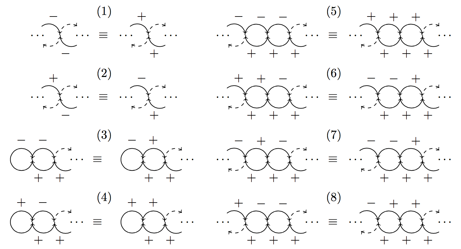
Figure 6: Table of $\oplus$-equivalences.

Isomorphism classes

Proposition 4.

The set of $\oplus$-BACCs of length $m$ and size $(n_{1},\ldots,n_{m})$ admits one isomorphism class if $m-1$ is not a multiple of $3$ and two if $m-1$ is a multiple of $3$.

As in the case of $\oplus$-BAFs, the proof of Proposition 4 is done in two steps.

• Point 1. We first show that the set of $\oplus$-BACCs of a given type $(n_{1},\ldots,n_{m})$ is divided into two classes: the positive class and the negative class, which respectively corresponds to the isomorphism class of the BACC $(n_{1},\ldots,n_{m})$ where all path are positive, and the isomorphism class of the BACC $(n_{1},\ldots,n_{m})$ where all paths are positive except the one from $i^{1}_{2}$ to $i^{1}_{1}$ that is negative.

• Point 2. We then prove that, in fact, when $m-1$ is not a multiple of $3$, the two classes coincide since the positive BACC and the negative BACC are isomorphic in this case.

The proof of these two points is based on the equivalences presented in Figure 6. Each pattern of these equivalences describes a subnetwork where every intersection automaton is a $\oplus$-automaton and every arc represents a signed path of arbitrary length (hence containing possibly several automata). These equivalences have to be understood as follows: given a BAN such that the left pattern of an equivalence appears in its interaction graph, then this BAN is behaviourally isomorphic to the BAN that has the same interaction graph except that the left pattern has been replaced by the right pattern of the equivalence, no matter what the outgoing dashed arcs are and no matter their number. In other words, Figure 6 presents a set of interaction graph rewriting rules that produce equivalent networks according to the (behavioural) isomorphism relation.

The following lemma (4) says in particular that it is enough to prove that the interaction graphs of two BANs can be rewritten one into an other using the equivalences from Figure 6, to prove that the two corresponding BANs are equivalent.

Lemma 4.

The interaction graph rewriting rules depicted in Figure 6 preserve the behavioural isomorphism equivalence.

Proof.

Equivalences (1) and (2) only translate the well known identities $b_{1}\oplus b_{2}=\overline{b_{1}}\oplus\overline{b_{2}}$ and $\overline{b_{1}}\oplus b_{2}=b_{1}\oplus\overline{b_{2}}$ for any Boolean values $b_{1}$ and $b_{2}$.

The proofs of the other equivalences are a bit longer but do not present any difficulty. We now present a proof for the third equivalence, proofs for the other equivalences are similar:

Let $\mathcal{N}=\{f_{i}\}$ and $\mathcal{N}^{\prime}=\{f_{i}^{\prime}\}$ be two BANs whose interaction graphs only differ by the pattern shown in Equivalence (3). We denote by $\mathcal{C}_{1}$, $\mathcal{C}_{2}$ the two cycles of the pattern. Similarly, $o_{1}$ and $o_{2}$ denote the intersection automata and $\mathcal{C}_{2}^{u}$ denotes the upper half-cycle of $\mathcal{C}_{2}$. We are going to prove that $\mathcal{N}$ and $\mathcal{N}^{\prime}$ are isomorphic by giving a bijection $\varphi:V\to V^{\prime}$ and a set of local bijections $\{\phi_{i}:\mathbb{B}\to\mathbb{B}\}_{i\in V}$ satisfying the conditions from Lemma 1.

Let $\varphi$ be the identity over the set of automata and let $\phi_{i}=neg_{\mathbb{B}}$ if $i\in\mathcal{C}_{1}\cup\mathcal{C}^{u}_{2}\cup\{o_{1}\}$ and $\phi_{i}=id_{\mathbb{B}}$ otherwise. We need to check that $\phi_{i}(f_{i}(x))=f^{\prime}_{i}(\phi_{i}(x))$ for all automata $i$ in the network. This is immediate for all automata that do not belong to $\mathcal{C}_{1}\cup\mathcal{C}^{u}_{2}\cup\{o_{1},o_{2}\}$ since for these automata we have used the identity everywhere. Now, if $i\in\mathcal{C}_{1}\cup\mathcal{C}^{u}_{2}$, then $\phi_{i}(f_{i}(x))=\phi_{i}(pred(i))=\overline{pred(i)}=\phi_{pred(i)}(pred(i))=f^{\prime}_{i}(\phi(x))$ and so the identity holds. Finally it remains to check that the identity holds for Automata $o_{1}$ and $o_{2}$. This is the case since:

1. $\phi_{o_{1}}(f_{o_{1}}(x))=\phi_{o_{1}}(\overline{pred_{1}(o_{1})}\oplus pred_{2}(o_{1}))$ $=\overline{\overline{pred_{1}(o_{1})}\oplus pred_{2}(o_{1})}$

   $=\overline{\phi_{pred_{1}(o_{1})}({pred_{1}(o_{1}))}\oplus\phi_{pred_{2}(o_{1})}(pred_{2}(o_{1}))}=f^{\prime}_{o_{1}}(\phi(x))$,

2. and

3. $\phi_{o_{2}}(f_{o_{2}}(x))=\phi_{o_{2}}(\overline{pred_{1}(o_{2})}\oplus pred_{2}(o_{2}))$ $=\overline{pred_{1}(o_{2})}\oplus pred_{2}(o_{2})$

   $=\phi_{pred_{1}(o_{2})}({pred_{1}(o_{2}))}\oplus\phi_{pred_{2}(o_{2})}(pred_{2}(o_{2}))$ $=f^{\prime}_{o_{2}}(\phi(x))$.

∎

Using the equivalence of Lemma 4 we can now finish the proof of Proposition 4. As mentioned above, we first show that the interaction graph of any $\oplus$-BACC can be rewritten into an interaction graph with at most one negative path from $i^{1}_{2}$ to $o_{1}(=i^{1}_{1})$. This proves that there are at most two isomorphism classes for a given $\oplus$-BACC type, the positive one and the negative one. Then we prove that if $m-1$ is not a multiple of $3$ this negative path can actually be removed by an other sequence of rewrites, hence proving that the two classes are equal in this case.

Proof.

(Point 1.) As usually we focus on canonical BANs, since this already reduces the number of cases to consider. Then using Equivalences (1) and (2) from Figure 6 we rewrite the interaction graph of any of the canonical $\oplus$-BACC into interaction graphs where the only negative paths are paths from $o_{i}$ to $o_{i+1}$ for $i\in\{1,\ldots,m-2\}$, that is, the only negative paths are “on the top”.

Then, inductively on the negative path of higher index (the negative path from $o_{i}$ to $o_{i+1}$ such that $i$ is maximal), we use the equivalences (5), (6), (7) and (8) from left to right to lower this index by at least one after every rewrite. We stop the rewriting when $i=0$ or when there are no negative paths left. In other words we do an inductive sequence of rewrites on the “right most” negative path so as to “push” this path to the left until reaching the end of the chain or making it disappear. An example of such a rewrite sequence is presented in Figure 7.

By Lemma 4 the above rewritings prove that any $\oplus$-BACC is isomorphic to a $\oplus$-BACC of same structure with at most two negative paths on its first two cycles. Finally the equivalences (3) and (4) reduce the four base cases ($++$,$+-$,$-+$,$--$) obtained this way to two: the positive case ($++$) and the negative case ($-+$). ∎

Proof.

(Point 2.) We now consider the interaction graph of a negative $\oplus$-BACC of length $m$. By Equivalence (2), this network is isomorphic to a $\oplus$-BACC of same structure with only one negative path on the first or on the second bottom half-cycle. Then, viewing the BACC upside-down, we can reuse the equivalences (6) and (8) alternatively so as to push this negative path to the right. Every time we apply the equivalences (6) and (8) successively the negative path is pushed 3 half-cycles to the right. Finally Equivalence (4) tells us that if the negative path is pushed to the second last bottom half-cycle then the $\oplus$-BACC is in the positive class. This can only happen if $m-1\equiv 1\mod(3)$ or if $m-2\equiv 1\mod(3)$, depending on if we start from the first or from the second bottom half-cycle respectively. In other words, this is the case if $m-1$ is not a multiple of $3$.

Moreover, the equivalences presented in Figure 6 are exhaustive, i.e. any other equivalences involving $\oplus$-chains can be deduced from these eight equivalences. So, the argument above also proves that a positive $\oplus$-BACC and a negative $\oplus$-BACC cannot be isomorphic unless $m-1$ is a multiple of $3$. In other words, if $m-1\equiv 0\mod(3)$ there are always two isomorphism classes, the positive one and the negative one. ∎

$\qquad\equiv\quad(1)$

$\qquad\equiv\quad(8)$

$\qquad\equiv\quad(8)$

Figure 7: Example of the rewrite of a cycle chain of type (1,2,2,2,2,2,1) into a negative cycle chain of type (1,2,2,2,2,2,1)

ATG

For every type of $\oplus$-BACCs, we now study the number of fixed points of each of their behavioural isomorphism classes so as to precise the general picture of their ATG given by Theorem 3.

Proposition 5.

A positive $\oplus$-BACC of length $m$ and size $n$ has a unique fixed point, $0^{n}$, if $(m-1)\not\equiv 0\mod(3)$ and has two fixed points, $0^{n}$ and $(101)^{\frac{m-1}{3}}$, if $(m-1)\equiv 0\mod(3)$. A negative $\oplus$-BACC (of length $m\equiv 1\mod(3)$) has no fixed point.

Proof.

In a stable configuration all the nodes of a given nude path have the same state, hence from now on we focus on determining the states of the intersection automata $o_{k}$. As this is done in Section 4.1 for $\oplus$-BAF, we determined the fixed points of a positive $\oplus$-BACC by fixing the state of one of its automata and propagating the information induced until having to make a new choice or reaching a fixed point or a contradiction. Here, we start by fixing Automaton $o_{1}$ (i.e. the “left most” automaton) and by induction on the two possible cases ($x_{o_{1}}=0$ and $x_{o_{1}}=1$) we show that this completely determines the state of the other automata if $x$ is a fixed point.

1. if $x_{o_{1}}=0$, then $o_{1}$ is stable if and only if $x_{o_{2}}=0$ and, recursively, for all $1<k\leqslant m-2$ , if $x_{o_{k-1}}=0$ and $x_{o_{k}}=0$ then $o_{k}$ is stable if and only if $x_{o_{k+1}}=0$. Hence $0^{m}$ is the unique fixed point such that $x_{0}=0$.

2. Similarly, if $x_{o_{1}}=1$ then $o_{1}$ is stable if and only if $x_{o_{2}}=0$. Then, we have three induction cases for all $1<k\leqslant m-2$: (1) if $x_{o_{k-1}}=1$ and $x_{o_{k}}=0$ then $o_{k}$ is stable if and only if $x_{o_{k+1}}=1$ ; (2) if $x_{o_{k-1}}=0$ and $x_{o_{k}}=1$ then $o_{k}$ is stable if and only if $x_{o_{k+1}}=1$; (3) if $x_{o_{k-1}}=1$ and $x_{o_{k}}=1$ then $o_{k}$ is stable if and only if $x_{o_{k+1}}=0$. Hence the only way for the last intersection automaton, $o_{m-1}$, to be stable when $x_{o_{1}}=1$ is that $(m-1)\equiv 0(\mod 3)$, and the corresponding configuration is $(101)^{(m-1)/3}$.

This concludes the proof of the first statement.

To show the second statement one only needs to realise that having a stable configuration for a negative $\oplus$-BACC of length $m\equiv 1\mod(3)$ amounts to having a stable configuration starting with a $1$ for a $\oplus$-BACC of size $m-1$, which is impossible from the proof above. Indeed, if $x_{o_{1}}=0$ then Automaton $o_{1}$ cannot be stable no matter the state value of Automaton $o_{2}$ in the configuration. Hence, if $x$ is a stable configuration $x_{o_{1}}$ must be $1$. This forces $x_{o_{2}}$ to be $1$ too (otherwise Automaton $o_{1}$ is not stable). So, if $x$ is stable then $x_{o_{2}}\ldots x_{o_{m}}$ is a stable configuration starting with a $1$ for a positive $\oplus$-BACC of size $m-1$. This is a contradiction. So there are no stable configurations for the negative $\oplus$-BACC of length $m\equiv 1\mod(3)$. ∎

According to Proposition 4, if $\mathcal{N}$ is a $\oplus$-BACC of length $m$ and size $n$ such that $m-1\neq 0\mod(3)$, then there is only one behavioural isomorphism class and so, similarly to what we have done for $\oplus$-BAFs, it is possible to characterise completely the ATG of $\mathcal{N}$ using Proposition 5: $G_{\mathcal{N}}^{A}$ has exactly one unreachable configuration, one fixed point, and one SCC of $2^{n}-2$ transient configurations.

The case where $m-1$ is a multiple of 3 is more complex because there are no easy ways to tell whether a network belongs to the positive or the negative class of its type, other than to compute its reduction graph as this is done in the proof of Proposition 4. Moreover, the class of the reverse network also depends on the length of each half-cycle in the $\oplus$-BACC, so describing each possible case would be tedious. However, summarising the results above, we can still state that there is at most two fixed points and two unreachable configurations in the transition graph of a $\oplus$-BACC of length $m-1\equiv 0\mod(3)$, or, to be more precise we can say that this transition graph has one of these four forms:

• a SCC of size $2^{n}-4$, two fixed points and two unstable configurations (case $\mathcal{N}$ and $\mathcal{N}^{R}$ are from the positive class);

• a SCC of size $2^{n}-2$ and two fixed points (case $\mathcal{N}$ is positive and $\mathcal{N}^{R}$ is negative);

• a SCC of size $2^{n}-2$ and two unreachable configurations (case $\mathcal{N}$ is negative and $\mathcal{N}^{R}$ is positive);

• a SCC of size $2^{n}$ (case both $\mathcal{N}$ and $\mathcal{N}^{R}$ are negative).

5 Interpretations and perspectives

Through general results and their application to particular classes of interaction graphs, the present work launches the description of asymptotic dynamical behaviours of $\oplus$-BANs under the asynchronous update mode. By this means, it contributes to improve our understanding of the wild domain of non-monotonic Boolean automata networks. Theorem 3 and Section 4 suggest for example that non local monotony brings both entropy and stability to BANs since the high expressiveness of the resulting networks helps them to converge to fix points instead of getting stuck into larger attractors. In the context of cellular reprogramming, the small number of attractors in $\oplus$-BANs as well as the small number of irreversible configurations suggest that the genes involved in a $\oplus$-cluster won’t be good candidates for being reprogramming determinants [2]. Hence this might help to reduce the number of genes to consider.

The notion of behavioural isomorphism also reveals to be a powerful tool for factorising proofs when it comes to the study of a particular family of BANs. Even if finding a proper set of interaction graph rewritings may be a bit challenging, it results in a very interesting and comprehensive tool that highlights which characteristics of the interaction graphs really matter in the dynamical behaviours of the BANs.

We believe that most of the results obtained could be refined or extended to some other types of ($\oplus$)-BANs. For example it should be possible to allow some arcs between or inside the cycles of a $\oplus$-BADC without changing the general shape of its corresponding ATG. These kinds of refinements draw a logical line for further works.

Another interesting question would be directed to the study and comparison of asymptotic behaviours under different update modes. From this perspective, the algorithms we describe and the ATG we get for strongly connected $\oplus$-BANs with an induced BADC of size greater than $3$ suggest that the addition of $k$-synchronism, that is when one allows $k$ automata to update simultaneously, make the set of unreachable configuration disappear if $k$ is greater than the size of the smallest cycle in an induced BADC of the network.

References

- [1] J. Aracena, A. Richard, and L. Salinas. Maximum number of fixed points in AND-OR-NOT networks. Journal of Computer and System Sciences, 80:1175–1190, 2014.
- [2] I. Crespo, T.M. Perumal, W. Jurkowski, and A. del Sol. Detecting cellular reprogramming determinants by differential stability analysis of gene regulatory networks. BMC Systems Biology, 7:140, 2013.
- [3] J. Demongeot, M. Noual, and S. Sené. Combinatorics of Boolean automata circuits dynamics. Discrete Applied Mathematics, 160:398–415, 2012.
- [4] G. Didier and É. Remy. Relations between gene regulatory networks and cell dynamics in Boolean models. Discrete Applied Mathematics, 160:2147–2157, 2012.
- [5] E. S. El-Mallah and C. J. Colbourn. The complexity of some edge deletion problems. IEEE Transactions on Circuits and Systems, 35:354–362, 1988.
- [6] M. Gadouleau, A. Richard, and É. Fanchon. Reduction and fixed points of Boolean networks and linear network coding solvability. 2014. Submitted (arXiv:1412.5310).
- [7] M. Gadouleau, A. Richard, and S. Riis. Fixed points of Boolean networks, guessing graphs, and coding theory. SIAM Journal on Discrete Mathematics, 2015. In press (arXiv:1409.6144).
- [8] C. Georgescu, W. J. R. Longabaugh, D. D. Scripture-Adams, E. David-Fung, M. A. Yui, M. A. Zarnegar, H. Bolouri, and E. V. Rothenberg. A gene regulatory network armature for T lymphocyte specification. Proceedings of the National Academy of Sciences, 105:20100–20105, 2008.
- [9] J. J. Hopfield. Neural networks and physical systems with emergent collective computational abilities. Proceedings of the National Academy of Sciences of the USA, 79:2554–2558, 1982.
- [10] J. J. Hopfield. Neurons with graded response have collective computational properties like those of two-state neurons. Proceedings of the National Academy of Sciences of the USA, 81:3088–3092, 1984.
- [11] A. S. Jarrah, R. Laubenbacher, and A. Veliz-Cuba. The dynamics of conjunctive and disjunctive Boolean network models. Bulletin of Mathematical Biology, 72:1425–1447, 2010.
- [12] S. A. Kauffman. Metabolic stability and epigenesis in randomly constructed genetic nets. Journal of Theoretical Biology, 22:437–467, 1969.
- [13] T. Melliti, M. Noual, D. Regnault, S. Sené, and J. Sobieraj. Asynchronous dynamics of Boolean automata double-cycles. In Proceedings of UCNC, volume 9252 of Lecture Notes in Computer Science, pages 250–262. Springer, 2015.
- [14] T. Melliti, D. Regrault, A. Richard, and S. Sené. On the convergence of Boolean automata networks without negative cycles. In Proceedings of Automata, volume LNCS 8155, pages 124–138. Springer, 2013.
- [15] L. Mendoza, D. Thieffry, and E. R. Alvarez-Buylla. Genetic control of flower morphogenesis in arabidopsis thaliana: a logical analysis. Bioinformatics, 15:593–606, 1999.
- [16] M. Noual. Synchronism vs asynchronism in boolean networks. arXiv:1104.4039, 2011.
- [17] M. Noual. Updating automata networks. PhD thesis, école normale supérieure de Lyon, 2012. http://tel.archives-ouvertes.fr/tel-00726560.
- [18] M. Noual, D. Regnault, and S. Sené. About non-monotony in Boolean automata networks. Theoretical Computer Science, 504:12–25, 2012.
- [19] M. Noual, D. Regnault, and S. Sené. Boolean networks synchronism sensitivity and XOR circulant networks convergence time. In Full Papers Proceedings of Automata’12, volume 90 of Electronic Proceedings in Theoretical Computer Science, pages 37–52. Open Publishing Association, 2012.
- [20] E. Remy, B. Mossé, C. Chaouiya, and D Thieffry. A description of dynamical graphs associated to elementary regulatory circuits. Bioinformatics, 19:172–178, 2003.
- [21] F. Robert. Discrete iterations: a metric study, volume 6 of Springer Series in Computational Mathematics. Springer, 1986.
- [22] D. Thieffry and R. Thomas. Dynamical behaviour of biological regulatory networks–ii. immunity control in bacteriophage lambda. Bulletin of mathematical biology, 57:277–97, 1995.
- [23] R. Thomas. Boolean formalization of genetic control circuits. Journal of Theoretical Biology, 42:563–585, 1973.