Schwinger mechanism revisited

Abstract

In this article, we review recent theoretical works on the Schwinger mechanism of particle production in external electrical fields. Although the non-perturbative Schwinger mechanism is at the center of this discussion, many of the approaches that we discuss can cope with general time and space dependent fields, and therefore also capture the perturbative contributions to particle production.

• Institut de physique théorique, CEA, CNRS, Université Paris Saclay
  F-91191 Gif-sur-Yvette, France

• Institut für Theoretische Physik, Universität Heidelberg
  Philosophenweg 16  D-69120, Heidelberg, Germany

1 Introduction

The Schwinger mechanism [1] is a non-perturbative phenomenon by which electron-positron pairs can be produced by a static electrical field [2, 3, 1]. It is the fact that the field is time independent that makes this process genuinely non-perturbative. Indeed, such an electromagnetic field can be viewed as an ensemble of photons of zero frequency, which by energy conservation are unable to produce massive particles. The non-perturbative nature of this phenomenon is visible in the fact that the corresponding transition amplitudes are non analytic in the coupling: since they are proportional to $\exp(-\pi m^{2}/eE)$, the coefficients of their Taylor expansion around $e^{2}=0$ are all zero, and only calculations to all orders in the coupling can make this effect manifest. The non-analytic behavior of these transition probabilities can be understood as a tunneling phenomenon (see for instance [4]) by which a particle from the Dirac sea is pulled into the positive energy states: as illustrated in the figure 1, the external gauge potential tilts the gap between the Dirac sea and the positive energy states, allowing a hole from the sea to tunnel through this gap and materialize as an on-shell positive energy particle on the other side.

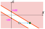
Figure 1: Schematic picture of the tunneling process involved in the Schwinger mechanism. The white band is the gap between the anti-electron Dirac sea and the positive energy electron continuum, tilted by the potential $V(x)=-Ex$ in the presence of an external electrical field $E$.

From this geometrical interpretation, it is clear that the length that needs to be crossed is inversely proportional to the electrical field, leading to a tunneling probability that is exponential in $1/E$.

From this pocket formula, we also see that the external field must be very intense in order to lead to a significant probability of particle production: at small coupling, this probability is of order one only for fields that are comparable to a critical field $E_{c}$ inversely proportional to the coupling constant, $E\sim E_{c}\equiv m^{2}/e$. Even for the lightest charged particle –the electron–, these are extremely intense fields that still surpass by several orders of magnitude the largest fields achievable experimentally. Note that when one studies the interaction of a charged particle with such an external electrical field, the corresponding expansion is in powers of $eE$. However, if $eE$ is comparable to the squared mass of the particle, then there is no small parameter to control this expansion and one must treat the external field to all orders. This is a prerequisite of any formalism aiming at describing the Schwinger mechanism.

Although the original derivation of the Schwinger mechanism was made in the context of quantum electrodynamics, it can be generalized to any quantum field theory coupled to some external field. In the context of strong interactions and quantum chromo-dynamics, where the coupling constant $g$ is numerically much larger than in QED, the production of pairs by the Schwinger mechanism may be achievable with more moderate chromo-electrical fields, and this phenomenon may play a role in the discussion of particle production in heavy ion collisions [5, 6, 7, 8], or in the decay of “hadronic strings” [9] in the process of hadronization. However, the gauge fields that are generated in heavy ion collisions have two important features: (i) since gauge fields have a direct coupling to gluons, the leading contributions for gluon production in heavy ion collisions are tree level contributions, that supersede the 1-loop contributions encountered in the Schwinger mechanism; (ii) these fields are in general space and time dependent [10, 11], and one must therefore use a formalism that can cope with the most general type of external field, without assuming any symmetry in its space-time dependence. Naturally, such fields generally imply that it is no longer possible to obtain closed analytic expressions (such analytical results have been obtained only for very special time dependences, and for spatial dependences that possess a high degree of symmetry). As a consequence, it is usually necessary to resort to numerical studies, and a recurrent concern in this review will be the practicality of various approaches for these numerical simulations.

The Schwinger mechanism can also be discussed in the context of a much simpler scalar field theory, coupled either to a scalar or vector external field (as in scalar QED). Despite its lack of connection to possible experimental realizations, this is the simplest example one may think of and it offers a very useful playground for testing new theoretical developments. In this review, we will often use such toy theories to illustrate various novel approaches, because of their didactic or phenomenological interest.

The outline of this review is as follows. In the section 2, we consider a scalar theory coupled to an external source and discuss particle production at tree level and 1-loop. The goal of this section is to present general ideas about these processes, whose range of validity is much broader than the simple toy model used to introduce them. The section 3 is devoted to a discussion of the multi-(anti)particle correlations that exist in the Schwinger mechanism. We first derive their general structure and then work it out in the special case of spatially homogeneous fields (possibly time dependent). The general discussion of the section 2 leads to a formulation of the Schwinger mechanism in terms of a complete basis of mode functions. In the section 4, we relate this representation to other approaches: the method of Bogoliubov transformations, the quantum kinetic equations, and the Wigner formalism, and we discuss lattice numerical implementations of this approach in the section 5. The section 6 is devoted to the worldline formalism, a radically different (but equivalent) formulation of the Schwinger formalism based on Schwinger’s proper-time representation of propagators in an external field. Besides new methods for calculating particle production in an external field, this approach provides a great deal of intuition on the spatio-temporal development of the production process. In the section 7, we discuss the idea of dynamically assisted Schwinger mechanism, where one superimposes two fields that have vastly different timescales and magnitudes in order to reach particle yields that are much larger than what would have been achieved with each field separately.

2 Quantum fields coupled to external sources

In this section, we discuss general aspects of quantum field theories coupled to an external source [12, 13]. Our main goal is to present the general aspects of such theories, focusing on their main differences with field theories where the sole interaction are the self-interaction of the fields. For the sake of simplicity, we consider a scalar field theory with a quartic self-interaction, whose Lagrangian is given by

$${\cal L}\equiv\frac{1}{2}(\partial_{\mu}\phi)(\partial^{\mu}\phi)-\frac{1}{2}m^{2}\phi^{2}-\frac{g^{2}}{4!}\phi^{4}+j\phi\;,$$ (1)

where $j(x^{0},{\bm{x}})$ is an unspecified function of space-time. Note that this source is a commuting number-valued object, rather than an operator. In the same way that one usually assumes that self-interactions are adiabatically turned on and off when $x^{0}\to\mp\infty$, we assume that the external source decreases fast enough when time goes to $\pm\infty$. Moreover, in order to preserve the unitarity of the theory, the external source must be real valued. Since this section is devoted to a general discussion, we allow the particles to have self-interactions. This is important for applications to gluon production in heavy ion collisions, and it leads to some complications. In contrast, the production of electron-positron pairs in QED is simpler to study because the electrons can only interact directly with the photon field. Interactions between electrons and positrons can happen indirectly, with the mediation of a photon, but this effect is an extremely small correction in practice, that would arise beyond the order considered here.

2.1 Vacuum diagrams

The main feature of such a theory is that it describes an open system: even if the system is initialized in the vacuum state that contains no particles, the external source can –and in general will– produce particles. This is in sharp contrast with the same theory in the vacuum, where the in- vacuum state and the out- vacuum state are related by a unitary transformation $\Omega(+\infty,-\infty)$ :

$$\big{|}0{}_{\rm out}\big{>}=\Omega(+\infty,-\infty)\,\big{|}0{}_{\rm in}\big{>}\qquad\qquad\mbox{(when $j\equiv 0$)}\;.$$ (2)

This property ensures that when $j\equiv 0$, the vacuum state evolves with probability one into the vacuum state, i.e. that no particle is created. An equivalent statement is that the vacuum to vacuum transition amplitude is a pure phase:

$$\big{<}0_{\rm out}\big{|}0{}_{\rm in}\big{>}=e^{i\,{\cal V}}\qquad\mbox{with ${\cal V}\in{\mathbbm{R}}$}\;.$$ (3)

This has some important practical consequences. The perturbative expansion for transition amplitudes generates diagrams that contain disconnected vacuum sub-diagrams, i.e. diagrams that have no external legs, but the above property tells us that the sum of all the vacuum diagrams is a pure phase that, although it appears as a prefactor in every transition amplitude, does not play any role after squaring the amplitudes in order to obtain transition probabilities. Therefore, it is legitimate to ignore from the start all the graphs that contain vacuum sub-diagrams in the $j\equiv 0$ case.

Let us return to the case $j\not=0$ and denote $P(\alpha)$ the transition probability from the initial vacuum state $\big{|}0{}_{\rm in}\big{>}$ to an arbitrary final state $\big{|}\alpha{}_{\rm out}\big{>}$. The unitarity of the theory implies that the sum of these probabilities over all the possible final states is equal to unity,

$$\sum_{\alpha}P(\alpha)=P(0)+\sum_{\alpha\not=0}P(\alpha)=1\;,$$ (4)

where in the first equality we have separated the vacuum and the populated states. If particles are produced during the time evolution of the system (this is possible only if $j\not=0$), then there is at least one non-empty state $\alpha$ for which $P(\alpha)>0$. Since all these probabilities are numbers in the range $[0,1]$, the previous identity implies that $P(0)<1$, i.e. that the vacuum does not evolve into the vacuum state with probability one anymore. A trivial consequence is that the vacuum to vacuum transition amplitude is no longer a pure phase, since its square is strictly smaller than unity. Because of this, it is no longer possible to disregard the vacuum graphs, as illustrated in the figure 2.

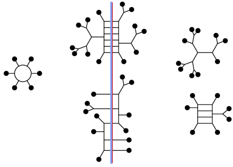
Figure 2: Example of diagram contribution to the probability of producing 11 particles (here illustrated in the case of a scalar theory with a cubic coupling to simplify the diagrams). The black dots denote the insertions of the external source $j(x)$. The vertical line indicates the final state (left of this line: amplitude, right: complex conjugated amplitude).

In general, this complicates considerably the diagrammatic expansion when $j\not=0$, but we will see later that inclusive quantities have a diagrammatic expansion made only of connected diagrams. Moreover, in the case of a strong external source (of order $1/g$), it becomes hopelessly complicated to calculate exclusive quantities (such as the probability $P(\alpha)$ for an individual final state) while the inclusive ones are much easier to access.

2.2 Power counting

In order to discuss ways of organizing the calculation of observables in field theories coupled to an external source, the first step is to assess the order of magnitude of a graph in terms of its topology. Obviously, for a graph with multiple disconnected components such as the one in the figure 2, the order is obtained as the product of the orders of each of its connected sub-diagrams. Therefore, it is sufficient to consider only connected graphs in this discussion. A connected diagram is fully characterized by the number of sources $n_{{}_{J}}$, the number of propagators $n_{{}_{P}}$, the number of vertices $n_{{}_{V}}$, the number of loops $n_{{}_{L}}$ and the number of external particles $n_{{}_{E}}$ (i.e. propagators endpoints that are not connected to a vertex or to a source). These quantities are not all independent. A first constraint comes from the fact that each propagator has two endpoints and each vertex receives four lines (for the scalar theory described by the Lagrangian of eq. (1)):

$$2n_{{}_{P}}=4n_{{}_{V}}+n_{{}_{J}}+n_{{}_{E}}\;.$$ (5)

A second identity expresses the number of independent loops $n_{{}_{L}}$ in terms of the other characteristics of the graph:

$$n_{{}_{L}}=n_{{}_{P}}-n_{{}_{E}}-n_{{}_{J}}-n_{{}_{V}}+1\;.$$ (6)

Thanks to these two formulas, the order of a connected graph can be written as

$$\omega(G)\equiv g^{2n_{{}_{V}}}\,j^{n_{{}_{J}}}=g^{-2+n_{{}_{E}}+2n_{{}_{L}}}\,(gj)^{n_{{}_{J}}}\;.$$ (7)

In this expression, we have combined one power of the coupling $g$ with each power of the external source $j$, because the combination $gj$ disappears from this power counting formula in the strong source regime where $j\sim g^{-1}$ (i.e. when particle production by the Schwinger mechanism becomes likely).

Eq. (7) displays a standard dependence on the number of loops and external legs. But it also indicates that in the strong source regime the dependence of the order on $n_{{}_{J}}$ disappears: therefore, infinitely many graphs contribute at each order. In conjunction with our previous observation that vacuum graphs cannot be disregarded, this poses a serious bookkeeping challenge for the calculation of quantities such as the transition probability shown on the figure 2.

2.3 Exclusive and inclusive quantities

Earlier, we have alluded to important differences between inclusive and exclusive observables when it comes to calculating them. Before going into these technical differences, let us first define them more precisely. Loosely speaking, exclusive observables are related to a full measurement of the final state, while inclusive observables involve dropping a lot of information about the final state.

If we assume the initial state to be empty, all the information about the final state is encoded in the transition amplitudes

$$\big{<}{\bm{p}}_{1}\cdots{\bm{p}}_{n}{}_{\rm out}\big{|}0{}_{\rm in}\big{>}$$ (8)

in which the final state is fully specified by giving the list of the momenta of all the final particles (in theories with more structure than the scalar theory under consideration in this section, one would also need to specify other quantum numbers of the final particles). Any observable related to this evolution can be expressed in terms of these amplitudes. For instance, the differential probability for producing $n$ particles can be expressed as

$$\frac{dP_{n}}{d^{3}{\bm{p}}_{1}\cdots d^{3}{\bm{p}}_{n}}=\frac{1}{n!}\frac{1}{(2\pi)^{3}2E_{{\bm{p}}_{1}}}\cdots\frac{1}{(2\pi)^{3}2E_{{\bm{p}}_{n}}}\,\big{|}\big{<}{\bm{p}}_{1}\cdots{\bm{p}}_{n}{}_{\rm out}\big{|}0{}_{\rm in}\big{>}\big{|}^{2}\;,$$ (9)

where $E_{\bm{p}}\equiv\sqrt{{\bm{p}}+m^{2}}$ is the on-shell energy of a particle of momentum ${\bm{p}}$. This quantity is called exclusive because only a single final state can contribute to it, at the exclusion of all others.

The archetype of inclusive observables are the particle spectra, obtained from the above probability distributions by integrating out the phase-space of all particles but a few. The simplest of them is the single particle spectrum, defined as

$$\frac{dN_{1}}{d^{3}{\bm{p}}}\equiv\sum_{n=0}^{\infty}(n+1)\int d^{3}{\bm{p}}_{1}\cdots d^{3}{\bm{p}}_{n}\;\frac{dP_{n+1}}{d^{3}{\bm{p}}d^{3}{\bm{p}}_{1}\cdots d^{3}{\bm{p}}_{n}}\;.$$ (10)

This quantity gives the number of particles (thanks to the factor $n+1$ included under the sum) produced in a given momentum range, but the information about the distribution of individual final states has been lost. As we shall see, this quantity is much easier to calculate than the exclusive observables. Experimentally, it is also much more accessible since it only requires to make an histogram of the momenta of the final state particles. The single particle spectrum has obvious generalizations: the 2-particle spectrum, the 3-particle spectrum, etc… that provide information about the correlations between the final state particles.

The “vacuum survival probability” often plays a special role in discussions of the Schwinger mechanism. This quantity is nothing but

$$P_{0}\equiv\big{|}\big{<}0{}_{\rm out}\big{|}0{}_{\rm in}\big{>}\big{|}^{2}\;.$$ (11)

A standard result in field theory is that the vacuum transition amplitude $\big{<}0{}_{\rm out}\big{|}0{}_{\rm in}\big{>}$ can be written as the exponential of the sum of the connected vacuum diagrams,

$$\big{<}0{}_{\rm out}\big{|}0{}_{\rm in}\big{>}=e^{i\,{\cal V}}\;,\qquad i\,{\cal V}\equiv\quad\;\raise-9.95845pt\hbox to199.16928pt{\leavevmode\resizebox{199.16928pt}{}{\includegraphics{vacuum-connected}}}$$ (12)

(Only a few tree level contributions to ${\cal V}$ have been shown in the illustration.) After squaring this amplitude, we get $P_{0}=\exp(-2\,{\rm Im}\,{\cal V})$. In the presence of an external source that remains constant over a long interval of time and is sufficiently spatially homogeneous, the imaginary part $2{\rm Im}\,{\cal V}$ can usually be written as an integral over space-time,

$$2{\rm Im}\,{\cal V}=\int d^{4}x\;(\cdots)\;,$$ (13)

and the integrand in this formula is often interpreted as the “particle production rate”. We will return on this interpretation later, as it not entirely accurate in general and can be a source of confusion.

2.4 Cutting rules and Schwinger-Keldysh formalism

Earlier in this section, we have seen that the imaginary part of the connected vacuum graphs, ${\rm Im}\,{\cal V}$, plays an important role in the expression of the transition probabilities. This imaginary part can be obtained from an extension of the standard Feynman rules known as Cutkosky’s cutting rules [14, 15]. Here, we do not re-derive these rules but simply state them as a recipe, that must be applied to every graph:

• Divide the nodes (vertices and sources) contained in the graph into a set of $+$ nodes and a set of $-$ nodes, in all the possible ways. It is customary to materialize diagrammatically these two sets of nodes by drawing a line (the “cut”) that divides the graph in two subgraphs. Even if the original graph is connected, the sub-graphs on each side of this cut do not have to be connected.

• The $+$ vertices give a factor $-ig^{2}$ and the $-$ vertices give a factor $+ig^{2}$. The $+$ sources give a factor $+ij(x)$ and the $-$ sources give a factor $-ij(x)$.

• Two nodes of types $\epsilon=\pm$ and $\epsilon^{\prime}=\pm$ are connected by a bare propagator $G^{0}_{\epsilon\epsilon^{\prime}}$. In momentum space, these four propagators read

  $$G_{++}^{0}(p) =\frac{i}{p^{2}-m^{2}+i\epsilon}\;, G_{--}^{0}(p) =\frac{-i}{p^{2}-m^{2}-i\epsilon}$$

  $$G_{+-}^{0}(p) =2\pi\theta(-p^{0})\delta(p^{2}-m^{2})\;, G_{-+}^{0}(p) =2\pi\theta(+p^{0})\delta(p^{2}-m^{2}) \;.$$ (14)

• Multiply the outcome of these rules by $1/2$.

The subgraph that involves only $+$ labels is obtained by the usual Feynman rules used to calculate transition amplitudes, while the $-$ subgraph is given by the complex conjugation of these rules. The interpretation of these cutting rules is straightforward: the $+$ sector corresponds to an amplitude and the $-$ sector to a complex conjugated amplitude, while the $+-$ and $-+$ propagators provide the phase-space integration for the (on-shell, hence the delta functions) final state particles.

In fact, these rules are the perturbative realization of the optical theorem, that stems from unitarity. If we write the $S$ matrix as $S\equiv 1+iT$, then $S^{\dagger}S=1$ can be rewritten as

$$i(T^{\dagger}-T)=T^{\dagger}T\;.$$ (15)

By taking the expectation value of this identity in the vacuum state and inserting a complete set of states in the right hand side, it leads to

$${\rm Im}\,\underbrace{\vphantom{\sum_{\alpha}}\big{<}0{}_{\rm in}\big{|}T\big{|}0{}_{\rm in}\big{>}}_{{\cal V}}=\frac{1}{2}\sum_{\alpha}\big{<}0{}_{\rm in}\big{|}T^{\dagger}\big{|}\alpha{}_{\rm in}\big{>}\big{<}\alpha{}_{\rm in}\big{|}T\big{|}0{}_{\rm in}\big{>}=\frac{1}{2}\underbrace{\sum_{\alpha}}_{+-}\underbrace{\vphantom{\sum_{\alpha}}\big{<}0{}_{\rm in}\big{|}\alpha{}_{\rm out}\big{>}}_{-\mbox{\scriptsize\ sector}}\underbrace{\vphantom{\sum_{\alpha}}\big{<}\alpha{}_{\rm out}\big{|}0{}_{\rm in}\big{>}}_{+\mbox{\scriptsize\ sector}}\;.$$ (16)

The factor $1/2$ in the right hand side of this identity is the origin of the rule iv above. The Schwinger-Keldysh [16, 17] formalism is essentially equivalent to Cutkosky’s cutting rules, but it is usually introduced as a tool for the perturbative calculation of squared matrix elements rather than as a technique for calculating the imaginary part of a scattering amplitude (however, the optical theorem states that the two are closely related).

2.5 General remarks on the distribution of produced particles

All the transition amplitudes such as (8) contain in their diagrammatic expansion the disconnected vacuum graphs, as shown in the example of the figure 2. In other words, one can pull out a factor $\exp(i{\cal V})$ in all these amplitudes, or a factor $\exp(-2\,{\rm Im}\,{\cal V})$ in squared amplitudes. From our previous power counting formula (7), we expect ${\rm Im}\,{\cal V}$ to start at the order $1/g^{2}$ in the strong source regime,

$$2{\rm Im}\,{\cal V}=\frac{a}{g^{2}}\;,\qquad P_{0}=e^{-a/g^{2}}\;,$$ (17)

where $a$ is an infinite series in powers of $g^{2n_{{}_{L}}}(gj)^{n_{{}_{J}}}$. At tree level ($n_{{}_{L}}=0$) and in the strong source regime, $a$ is therefore of order unity (but depends non-perturbatively on the source).

Let us now turn to the probabilities of producing particles. Besides the factor $\exp(i{\cal V})$, the transition amplitude from the vacuum to a state containing one particle is made of graphs that connect sources to a single final particle. From eq. (7), these graphs start at the order $g^{-1}$, and the leading contribution to $P_{1}$ is of the form

$$P_{1}=e^{-a/g^{2}}\;\Big{[}\frac{b_{1}}{g^{2}}\Big{]}\;,$$ (18)

where $b_{1}/g^{2}$ is the sum of the 1-particle cuts (i.e. cuts that cut exactly one propagator) through connected vacuum diagrams. Its diagrammatic expansion starts with the following terms

$$\frac{b_{1}}{g^{2}} =$$ (19)

$$+\cdots\;.$$

The probability $P_{2}$ of producing two particles is a bit more complicated. It contains a term $(b_{1}/g^{2})^{2}/2!$ corresponding to the independent emission of two particles (the factor $1/2!$ is a symmetry factor due to the fact that the two particles are indistinguishable) and an additional term $b_{2}/g^{2}$ in which the two particles are correlated:

$$P_{2}=e^{-a/g^{2}}\;\left[\frac{1}{2!}\frac{b_{1}^{2}}{g^{4}}+\frac{b_{2}}{g^{2}}\right]\;.$$ (20)

The quantity $b_{2}/g^{2}$ can be obtained as the sum of the 2-particle cuts of connected vacuum diagrams:

$$\frac{b_{2}}{g^{2}} =$$ (21)

$$+\cdots$$

Likewise, the probability $P_{3}$ of producing 3 particles reads

$$P_{3}=e^{-a/g^{2}}\;\left[\frac{1}{3!}\frac{b_{1}^{3}}{g^{6}}+\frac{b_{1}b_{2}}{g^{4}}+\frac{b_{3}}{g^{2}}\right]\;,$$ (22)

where the last term is the sum of the 3-particle cuts of connected vacuum diagrams

$$\frac{b_{3}}{g^{2}} =$$ (23)

$$+\cdots$$

The previous examples can be generalized easily into a formula for the probability of producing $n$ particles,

$$P_{n}=e^{-a/g^{2}}\;\sum_{p=1}^{n}\frac{1}{p!}\sum_{r_{1}+\cdots+r_{p}=n}\frac{b_{r_{1}}\cdots b_{r_{p}}}{g^{2p}}\;.$$ (24)

In this formula, $p$ is the number of clusters (sets of correlated particles) into which the $n$ particles can be divided. Note that, except for the powers of $g^{2}$ that indicate the order of each term in the strong source regime, this formula is completely generic and does not depend on the details of the field theory under consideration: it just expresses the combinatorics of grouping $n$ objects into $p$ clusters. Let us end this subsection by noting that unitarity requires that $a=b_{1}+b_{2}+b_{3}+\cdots$ (this identity can be viewed as a consequence of the optical theorem, since $a/g^{2}$ is $2\,{\rm Im}\,({\cal V})$ and $(b_{1}+b_{2}+b_{3}+...)/g^{2}$ is the sum of all the cuts through ${\cal V}$).

2.6 Generating functional

So far, our discussion has been at a rather qualitative level. We now turn to a more detailed discussion of what quantities can be calculated and of what tools can do it. For bookkeeping purposes, it is useful to introduce the following generating functional,

$${\cal F}[z({\bm{p}})]\!\equiv\!\!\sum_{n=0}^{\infty}\!\frac{1}{n!}\!\int\!\!\frac{d^{3}{\bm{p}}_{1}}{(2\pi)^{3}2E_{{\bm{p}}_{1}}}\cdots\frac{d^{3}{\bm{p}}_{n}}{(2\pi)^{3}2E_{{\bm{p}}_{n}}}\,z({\bm{p}}_{1})\cdots z({\bm{p}}_{n})\,\left|\big{<}{\bm{p}}_{1}\cdots{\bm{p}}_{n}{}_{\rm out}\big{|}0_{\rm in}\big{>}\right|^{2}\!\!,$$ (25)

where $z({\bm{p}})$ is a test function over the 1-particle phase-space. Any observable which is expressible in terms of the transition amplitudes (8) can be obtained from derivatives of ${\cal F}[z({\bm{p}})]$. In particular, the differential probabilities and the single particle spectrum are obtained as:

$$\frac{dP_{n}}{d^{3}{\bm{p}}_{1}\cdots d^{3}{\bm{p}}_{n}} = \frac{1}{n!}\left.\frac{\delta^{n}{\cal F}[{\bm{z}}({\bm{p}})]}{\delta z({\bm{p}}_{1})\cdots\delta z({\bm{p}}_{n})}\right|_{{\bm{z}}({\bm{p}})=0}\;,$$

$$\frac{dN_{1}}{d^{3}{\bm{p}}} = \left.\frac{\delta{\cal F}[z({\bm{p}})]}{\delta z({\bm{p}})}\right|_{z({\bm{p}})=1}\;.$$ (26)

As one can see on these two examples, observables in which the final state is fully specified correspond to derivatives evaluated at $z({\bm{p}})=0$ (which eliminates most of the final states from the sum in eq. (25)), while inclusive observables –in which all the final states are kept and most of their particles are integrated out– correspond to derivatives evaluated at $z({\bm{p}})=1$. This is in fact a general property. For instance, the 2-particle spectrum is

$$\frac{dN_{2}}{d^{3}{\bm{p}}d^{3}{\bm{q}}}=\left.\frac{\delta^{2}{\cal F}[{\bm{z}}({\bm{p}})]}{\delta z({\bm{p}})\delta z({\bm{q}})}\right|_{z({\bm{p}})=1}\;,$$ (27)

and this formula has an obvious generalization to the case of the inclusive $n$-particle spectrum.

As we shall see, inclusive observables are much simpler to calculate than the exclusive ones. To a large extent, this simplification is due to unitarity. The simplest consequence of unitarity is

$${\cal F}[z({\bm{p}})=1]=1\;.$$ (28)

At $z({\bm{p}})=0$, one would have instead obtained ${\cal F}[z({\bm{p}})=0]=P_{0}$, which is a very complicated object. These considerations show that it is much simpler to study the generating functional near the point $z({\bm{p}})=1$ than near the point $z({\bm{p}})=0$. In terms of a diagrams, the identity (28) corresponds to an exact cancellation among an infinite set of diagrams when one evaluates ${\cal F}[z({\bm{p}})]$ at $z({\bm{p}})=1$.

The reason why we discussed at length vacuum-vacuum diagrams in the previous subsection is that they play an important role in organizing the calculation of other quantities. The key observation here is that the sum of the vacuum-vacuum diagrams is nothing but the generating functional for time-ordered Green’s functions. More precisely, one has

$$\big{<}0_{\rm out}\big{|}{\rm T}\,\phi(x_{1})\cdots\phi(x_{n})\big{|}0_{\rm in}\big{>}=\frac{\delta}{i\delta\eta(x_{1})}\cdots\frac{\delta}{i\delta\eta(x_{n})}\;\left.e^{i\,{\cal V}[j+\eta]}\right|_{\eta=0}\;,$$ (29)

where the notation ${\cal V}[j+\eta]$ indicates that one should evaluate the connected vacuum diagrams with a fictitious source $\eta$ added to the physical source $j$. The fictitious source is set to zero after having performed the functional differentiations.

Then, it is easy to obtain a formal but useful formula for ${\cal F}[z({\bm{p}})]$. Start from the Lehmann–Symanzik–Zimmermann [4] reduction formula for the transition amplitude to a final state with $n$ particles,

$$\big{<}{\bm{p}}_{1}\cdots{\bm{p}}_{n}{}_{\rm out}\big{|}0{}_{\rm in}\big{>} = i^{n}\int d^{4}x_{1}\cdots d^{4}x_{n}\;e^{i(p_{1}\cdot x_{1}+\cdots+p_{n}\cdot x_{n})}$$ (30)

$$\quad\times(\square_{x_{1}}+m^{2})\cdots(\square_{x_{n}}+m^{2})\;\big{<}0_{\rm out}\big{|}{\rm T}\,\phi(x_{1})\cdots\phi(x_{n})\big{|}0_{\rm in}\big{>}\;.$$

By plugging eq. (29) in this reduction formula and squaring the result, we can write the squared amplitude as

$$\left|\big{<}{\bm{p}}_{1}\cdots{\bm{p}}_{n}{}_{\rm out}\big{|}0{}_{\rm in}\big{>}\right|^{2}=\left.{\cal C}_{{\bm{p}}_{1}}\cdots{\cal C}_{{\bm{p}}_{n}}\;e^{i{\cal V}[j+\eta_{+}]}\,e^{-i{\cal V}^{*}[j+\eta_{-}]}\right|_{\eta_{\pm}=0}\;,$$ (31)

where the operator ${\cal C}_{\bm{p}}$ is defined by

$${\cal C}_{\bm{p}}\equiv\int d^{4}xd^{4}y\;e^{ip\cdot(x-y)}\;(\square_{x}+m^{2})(\square_{y}+m^{2})\;\frac{\delta^{2}}{\delta\eta_{+}(x)\delta\eta_{-}(y)}\;.$$ (32)

In the right hand side of eq. (31), the factors $\exp(i{\cal V})$ and $\exp(-i{\cal V}^{*})$ come respectively from the amplitude and its complex conjugate. Note that it is essential to keep their arguments distinct–hence the separate $\eta_{+}$ and $\eta_{-}$–so that the two derivatives in the operators ${\cal C}_{\bm{p}}$ act on different factors. One should set $\eta_{\pm}$ to zero only after all the derivatives have been evaluated. The final step is to substitute eq. (31) into the definition (25) of ${\cal F}[z({\bm{p}})]$. One obtains immediately

$${\cal F}[z({\bm{p}})]=\left.\exp\left[\int\frac{d^{3}{\bm{p}}}{(2\pi)^{3}2E_{\bm{p}}}\;z({\bm{p}})\,{\cal C}_{\bm{p}}\right]\;e^{i{\cal V}[j+\eta_{+}]}\,e^{-i{\cal V}^{*}[j+\eta_{-}]}\right|_{\eta_{\pm}=0}\;.$$ (33)

From this formula, one can show that the generating functional ${\cal F}[z({\bm{p}})]$ is the sum of all the vacuum diagrams in a modified Schwinger-Keldysh formalism in which all the off-diagonal ($G_{+-}^{0}(p)$ and $G_{-+}^{0}(p)$) propagators are multiplied by $z({\bm{p}})$.

There is no simple expression for the generating functional ${\cal F}[z({\bm{p}})]$ itself, but it turns out that it is much easier to obtain a formula for its first derivative $\delta{\cal F}[z({\bm{p}})]/\delta z({\bm{p}})$. Using eq. (33) and the explicit form of the operator ${\cal C}_{\bm{p}}$, we can write this derivative as

$$\frac{\delta\ln{\cal F}[z({\bm{p}})]}{\delta z({\bm{p}})} = \smash{\frac{1}{(2\pi)^{3}2E_{\bm{p}}}\int}d^{4}xd^{4}y\;e^{ip\cdot(x-y)}\;(\square_{x}+m^{2})(\square_{y}+m^{2})$$ (34)

$$\qquad\qquad\qquad\qquad\qquad\times\,\Big{[}\varphi_{+}(x)\varphi_{-}(y)+{\cal G}_{+-}(x,y)\Big{]}\;.$$

where $\varphi_{\pm}(x)$ and ${\cal G}_{+-}(x,y)$ are the connected 1-point and 2-point Green’s functions in this modified Schwinger-Keldysh formalism, respectively (they implicitly depend on the external source $j$ and on the test function $z({\bm{p}})$), as illustrated in the figure 3.

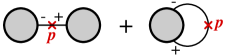
Figure 3: Schematic diagrammatic representation of the two contributions to the derivative of the generating functions. Left: term in $\varphi_{+}\varphi_{-}$. Right: term in ${\cal G}_{+-}$.

The order of magnitude of these objects is easily obtained from our general results for the power counting of connected graphs :

$$\varphi_{\pm} \sim {\cal O}(g^{-1})\;,$$

$${\cal G}_{+-} \sim {\cal O}(1)\;.$$ (35)

Therefore, the first derivative of $\ln{\cal F}[z({\bm{p}})]$ starts at the order $g^{-2}$. Moreover, at this order, only the first term in $\varphi_{+}(x)\varphi_{-}(y)$ contributes. The term in ${\cal G}_{+-}$ starts contributing only at the next-to-leading order. A further simplification at leading order is that it is sufficient to keep tree level contributions to the 1-point functions $\varphi_{\pm}$. Thanks to this tree structure, the functions $\varphi_{\pm}$ at Leading Order are solutions of the classical equation of motion,

$$(\square_{x}+m^{2})\varphi_{\pm}(x)+U^{\prime}(\varphi_{\pm}(x))=j(x)\;,$$ (36)

where $U^{\prime}$ is the first derivative of the interaction potential (e.g. $U^{\prime}(\varphi)=g^{2}\varphi^{3}/6$ in the scalar model considered in this section). This equation depends on the external source $j(x)$, but not on the test function $z({\bm{p}})$. The latter comes only via the boundary conditions

$$f_{+}^{(+)}(-\infty,{\bm{p}}) = f_{-}^{(-)}(-\infty,{\bm{p}})=0\;,$$

$$f_{+}^{(-)}(+\infty,{\bm{p}}) = z({\bm{p}})\;f_{-}^{(-)}(+\infty,{\bm{p}})\;,$$

$$f_{-}^{(+)}(+\infty,{\bm{p}}) = z({\bm{p}})\;f_{+}^{(+)}(+\infty,{\bm{p}})\;.$$ (37)

In these equations, the boundary conditions have been written in terms of the coefficients of the Fourier decomposition of the fields $\varphi_{\pm}$,

$$\varphi_{\epsilon}(y)\equiv\int\frac{d^{3}{\bm{p}}}{(2\pi)^{3}2E_{\bm{p}}}\;\Big{[}f_{\epsilon}^{(+)}(y^{0},{\bm{p}})\,e^{-ip\cdot y}+f_{\epsilon}^{(-)}(y^{0},{\bm{p}})\,e^{+ip\cdot y}\Big{]}\;.$$ (38)

(The Fourier coefficients are time dependent because $\varphi_{\pm}$ are not free fields.)

By plugging the Fourier representation of $\varphi_{\pm}$ in the general formula (34) (and setting ${\cal G}_{+-}=0$ at this order), we get a very simple formula for the first derivative of $\ln{\cal F}[z({\bm{p}})]$ at leading order:

$$\left.\frac{\delta\ln{\cal F}[z({\bm{p}})]}{\delta z({\bm{p}})}\right|_{{}_{\rm LO}}=\frac{1}{(2\pi)^{3}2E_{\bm{p}}}\;f_{+}^{(+)}(+\infty,{\bm{p}})\,f_{-}^{(-)}(+\infty,{\bm{p}})\;.$$ (39)

Note that it is in general extremely difficult to solve the non-linear partial differential equation (36) with boundary conditions imposed both at $x^{0}=-\infty$ and at $x^{0}=+\infty$, as in eqs. (37). Therefore, one should not hope to be able to find solutions of this problem (either analytically or numerically). As we shall see later, the only exception is when the fields under consideration do not have self-interactions but are solely driven by the external source. This is for instance the case for fermion production under the influence of an external electromagnetic field. Nevertheless, this result for the first derivative of the generating functional ${\cal F}[z({\bm{p}})]$ is very useful as an intermediate tool for deriving other results, as will be shown in the rest of this section.

2.7 Inclusive quantities at leading order (tree level)

2.7.1 Single particle spectrum

Let us now show how to obtain inclusive moments (for now, at leading order) from eq. (39). The simplest one is the single inclusive spectrum. At leading order, it is simply obtained by evaluating eq. (39) at the special point $z({\bm{p}})=1$, since ${\cal F}[z({\bm{p}})=1]=1$. This means that one must solve the classical equation of motion with boundary conditions (37) in which one sets $z({\bm{p}})=1$. Setting $z({\bm{p}})=1$ in these boundary conditions simplifies them considerably: the two fields $\varphi_{+}$ and $\varphi_{-}$ are identical,

$$\mbox{if\ }z({\bm{p}})\equiv 1\;,\qquad\varphi_{+}(x)=\varphi_{-}(x)\equiv\varphi(x)\;,$$ (40)

and obey the simple retarded boundary condition

$$\lim_{x^{0}\to-\infty}\varphi(x^{0},{\bm{x}})=0\;,\qquad\lim_{x^{0}\to-\infty}\partial^{0}\varphi(x^{0},{\bm{x}})=0\;.$$ (41)

Thus, the prescription for computing the single inclusive spectrum at leading order is the following:

• Solve the classical field equation of motion with a null initial condition in the remote past,

• At $x^{0}\to+\infty$, compute the coefficients  $f^{(\pm)}(+\infty,{\bm{p}})$ of the Fourier decomposition of this classical field,

• The single inclusive spectrum is then obtained as:

  $$\left.\frac{dN_{1}}{d^{3}{\bm{p}}}\right|_{{}_{\rm LO}}=\frac{1}{(2\pi)^{3}2E_{\bm{p}}}\;\left|f^{(+)}(+\infty,{\bm{p}})\right|^{2}\;.$$ (42)

In eq. (42), we have used the fact that the retarded classical field $\varphi$ is purely real . Since in the step i the boundary conditions are retarded, this problem is straightforward to solve, at least numerically. A few important comments are in order here:

• If the fields are not self-interacting, then the single particle spectrum is simply the square of the Fourier coefficients of the source itself.

• If the source has only space-like Fourier modes (this happens if there is frame in which it is time independent), then this is also the case for the solution of the classical equation of motion (36), and the single particle spectrum is zero at leading order.

• This leading order contribution can only exist if the field under consideration is directly coupled to the external source. For instance, the direct production of electrons from an electromagnetic current is impossible at this order, but can happen at next-to-leading order (the current couples to an electron-positron pair, but this requires an extra coupling constant).

This is the form that gluon production takes in the Color Glass Condensate framework [18, 19, 20, 21, 22, 23, 24, 25] when applied to heavy ion collisions. In this effective description of high energy nucleus-nucleus collisions, the color gauge fields are coupled to two external currents that represent the color charges carried by the fast partons of the incoming nuclei. At high energy, it is expected that the gluon occupation number in nuclei may reach non-perturbative values of order $1/g^{2}$, which would correspond to strong sources in the sense used in this section. The spectrum of produced gluons at leading order in this description is obtained from the retarded classical solutions of the Yang-Mills equations,

$$\big{[}D_{\mu},F^{\mu\nu}\big{]}=J_{1}^{\nu}+J_{2}^{\nu}\;,$$ (43)

where $J_{1}^{\nu}$ and $J_{2}^{\nu}$ are the color currents of the two projectiles. This approach has been implemented in a number of works [26, 27, 28, 29, 30, 31, 32, 33], and is now included in the IP-glasma model for the matter produced immediately after such a collision [34].

2.7.2 Multi-particle spectra

The $n$-particle inclusive spectrum is also obtained from derivatives of the generating functional ${\cal F}[z(p)]$ evaluated at $z({\bm{p}})=1$,

$$\frac{dN_{n}}{d^{3}{\bm{p}}_{1}\cdots d^{3}{\bm{p}}_{n}}=\left.\frac{\delta^{n}{\cal F}[z({\bm{p}})]}{\delta z({\bm{p}}_{1})\cdots\delta z({\bm{p}}_{n})}\right|_{z({\bm{p}})=1}\;,$$ (44)

that can equivalently be written as :

$$\frac{dN_{n}}{d^{3}{\bm{p}}_{1}\cdots d^{3}{\bm{p}}_{n}}=\prod_{i=1}^{n}\left[\frac{\delta\ln{\cal F}}{\delta z(p_{i})}\right]_{z({\bm{p}})=1}+\sum_{i<j}\left[\frac{\delta^{2}\ln{\cal F}}{\delta z(p_{i})\delta z({\bm{p}}_{j})}\right]_{z({\bm{p}})=1}\prod_{k\not=i,j}\left[\frac{\delta\ln{\cal F}}{\delta z(p_{k})}\right]_{z({\bm{p}})=1}+\cdots$$ (45)

The terms we have not written explicitly contain increasingly high order derivatives (but less and less factors), up to a single factor with an $n$-th derivative. However, these terms are not needed. Indeed, we already know that at leading order $\ln{\cal F}$ is of order $g^{-2}$ since it is a sum of connected vacuum-vacuum diagrams. Therefore, in the right hand side of this equation, the first term is of order $g^{-2n}$, the second term is of order $g^{-2(n-1)}$, etc… The leading contribution is thus the first term, and all the subsequent terms are subleading . We see that, at leading order, the $n$-particle inclusive spectrum is simply the product of $n$ single particle spectra:

$$\left.\frac{dN_{n}}{d^{3}{\bm{p}}_{1}\cdots d^{3}{\bm{p}}_{n}}\right|_{{}_{\rm LO}}=\prod_{i=1}^{n}\left.\frac{dN_{1}}{d^{3}{\bm{p}}_{i}}\right|_{{}_{\rm LO}}\;.$$ (46)

Any deviation from this factorized result is a subleading effect. Note also that at leading order, there is no difference between the factorial moments $\big{<}N(N-1)\cdots(N-n+1)\big{>}$ and the ordinary moments $\big{<}N^{n}\big{>}$. Moreover, at this order, the multiplicity distribution cannot be distinguished from a Poisson distribution.

In the Color Glass Condensate framework at leading order, the correlations among the produced particles can either originate from correlations that pre-exist in the distribution of the color sources that produce the gauge field [35, 36], or be built up at a later stage of the evolution of the system through collective motion of the produced particles (e.g. radial hydrodynamical flow [37, 38]). In heavy ion collisions, strong correlations have been observed between pairs of hadrons [39, 40, 41, 42], characterized by a ridge shape, very elongated in the relative rapidity of the two particles, and peaked in their relative azimuthal angle. By causality, the correlations in rapidity have to be created in the very early stages of the collisions [43], and they can be simply understood as a consequence of the near boost invariance of the sources of the incoming nuclei. In contrast, the azimuthal correlations can be produced at any time, and are easily explainable by the hydrodynamical flow that develops in the later stages of the collision process [44, 45].

2.8 Exclusive quantities at leading order

Let us now consider exclusive quantities. This discussion will be very short, and its purpose is only to illustrate the fact that the calculation of exclusive quantities is considerably more difficult than that of inclusive quantities. Let us consider as an example the calculation of the differential probability for producing exactly one particle. It may be obtained from ${\cal F}[z({\bm{p}})]$ by the formula

$$\frac{dP_{1}}{d^{3}{\bm{p}}}=\left.\frac{\delta{\cal F}[z({\bm{p}})]}{\delta z({\bm{p}})}\right|_{z({\bm{p}})=0}=\underbrace{{\cal F}[z({\bm{p}})=0]}_{\displaystyle{P_{0}}}\;\left.\frac{\delta\ln{\cal F}[z({\bm{p}})]}{\delta z({\bm{p}})}\right|_{z({\bm{p}})=0}\;.$$ (47)

There are two major differences compared to the inclusive spectra studied in the previous section :

• The derivative of $\ln{\cal F}[z({\bm{p}})]$ must be evaluated at the point $z({\bm{p}})=0$. At leading order, it can still be expressed in terms of the Fourier coefficients of a pair of solutions of the classical equation of motion, via eq. (39). However, because we must now set $z({\bm{p}})=0$ in the boundary conditions (37) for these classical fields, they are not retarded fields anymore, and there is no practical way to calculate them.

• The quantity ${\cal F}[z({\bm{p}})=0]$ appears as a prefactor in front of all the exclusive quantities. This prefactor is nothing but the probability $P_{0}$ for not producing anything, i.e. the vacuum survival probability. Calculating $P_{0}$ directly is a very difficult task. However, if one were able to calculate the second factor for all the probabilities $P_{1},P_{2},\cdots$, one could then obtain $P_{0}$ from the unitarity condition $\sum_{n=0}^{\infty}P_{n}=1$.

These difficulties, observed here on the example of $dP_{1}/d^{3}{\bm{p}}$, are in fact generic for all exclusive quantities. Note however that this is to a large extent an academic problem, since exclusive quantities –where one specifies in minute detail the final state– are not very interesting for the phenomenology of processes in which the final state has typically a very large number of particles, parametrically of order $g^{-2}$. Indeed, in this context, the probability of occurrence of a given fully specified final state is exponentially suppressed, like $e^{-c/g^{2}}$.

2.9 Particle production at next-to-Leading order (one loop)

In situations where the particles under consideration couple directly to a time dependent external source, these particles can be produced by the leading order mechanism described in the previous subsections, and the moments of the particle distribution are expressible in terms of the classical field generated by this source. However, when this direct coupling does not exist or when the external source is static, the production of particles is impossible at this order and can at best happen at the next-to-leading order in the coupling. This is in particular the case in the traditional setup of the Schwinger mechanism, where an electromagnetic current couples indirectly to fermion pairs via an electromagnetic field. Therefore, our goal in this subsection is not to calculate the subleading corrections to particle spectra in general, but to calculate the first nonzero contributions they receive when the leading order contribution vanishes.

In this subsection, we discuss the new production mechanisms that arise at NLO, by considering the single particle spectrum at 1-loop. This spectrum is given by the first derivative of the generating functional ${\cal F}[z({\bm{p}})]$, for which a general formula was given in eq. (34). At NLO, i.e. at the order $g^{0}$, it involves two quantities [46]:

• The 1-loop corrections $\beta_{\pm}$ to the 1-point functions $\varphi_{\pm}$,

• The 2-point function ${\cal G}_{+-}$ at tree level.

However, since we are interested in the NLO corrections only in cases where the leading order is zero, we do not need to evaluate the terms that contain $\beta_{\pm}$. Indeed, $\beta_{\pm}$ being a 1-loop correction to $\varphi_{\pm}$, it also leads to a vanishing contribution for static sources or if the particles of interest cannot couple directly to the external source. Therefore, only the second term is needed. This term corresponds to the production of a pair of particles from the external source (in the case of the single particle spectrum, one of the two produced particles is integrated out). Moreover, since we are not going to calculate further derivatives with respect to $z({\bm{p}})$, it is sufficient to evaluate this quantity at the point $z({\bm{p}})=1$ – which simplifies considerably the calculation. This NLO correction to the single inclusive spectrum reads

$$\left.\frac{dN_{1}}{d^{3}{\bm{p}}}\right|_{{}_{\rm NLO}}=\frac{1}{(2\pi)^{3}2E_{\bm{p}}}\int d^{4}xd^{4}y\;e^{ip\cdot(x-y)}\;(\square_{x}+m^{2})(\square_{y}+m^{2})\;{\cal G}_{+-}(x,y)\;.$$ (48)

The 2-point function ${\cal G}_{+-}(x,y)$ at tree level obeys the following integral equation :

$${\cal G}_{\epsilon\epsilon^{\prime}}(x,y)=G_{\epsilon\epsilon^{\prime}}^{0}(x,y)-i\sum_{\eta=\pm}\eta\int d^{4}z\;G_{\epsilon\eta}^{0}(x,z)\,U^{\prime\prime}(\varphi(z))\,{\cal G}_{\eta\epsilon^{\prime}}(z,y)\;,$$ (49)

and therefore mixes with the other three components, ${\cal G}_{-+}$, ${\cal G}_{++}$ and ${\cal G}_{--}$. Here, $-iU^{\prime\prime}(\varphi(z))$ is the general form for the insertion of a background field on a propagator in a theory with a potential $U(\varphi)$. From these equations, one can obtain the following formulas :

$${\cal G}_{+-}(x,y) = \int\frac{d^{3}{\bm{p}}}{(2\pi)^{3}2E_{\bm{p}}}\;a_{\bm{p}}^{*}(x)a_{\bm{p}}(y)\;,$$

$${\cal G}_{-+}(x,y) = \int\frac{d^{3}{\bm{p}}}{(2\pi)^{3}2E_{\bm{p}}}\;a_{\bm{p}}(x)a_{\bm{p}}^{*}(y)\;,$$ (50)

where the functions $a_{\bm{p}}(x)$ are mode functions defined by

$$\big{[}\square_{x}+m^{2}+U^{\prime\prime}(\varphi(x))\big{]}\,a_{\bm{p}}(x)=0\;,\quad\lim_{x^{0}\to-\infty}a_{\bm{p}}(x)=e^{ip\cdot x}\;.$$ (51)

Thus, the problem of finding the Schwinger-Keldysh propagators in a background field can be reduced to determining how plane waves propagate on top of the classical background field (and are distorted by this field). In the previous formulas, we have used the plane wave basis, but other choices are possible, as long as one chooses a properly normalized complete basis. Note also that the 4-dimensional space-time integrals in eq. (48) can in fact be rewritten as purely spatial integrals on a constant-$t$ surface (with $t\to+\infty$),

$$\left.\frac{dN_{1}}{d^{3}{\bm{p}}}\right|_{{}_{\rm NLO}}=\frac{1}{(2\pi)^{3}2E_{\bm{p}}}\int\frac{d^{3}{\bm{k}}}{(2\pi)^{3}2E_{\bm{k}}}\;\lim_{t\to+\infty}\left|\int d^{3}{\bm{x}}\;e^{-i{\bm{p}}\cdot{\bm{x}}}\;(\partial_{t}-iE_{\bm{p}})\;a_{\bm{k}}(x)\right|^{2}\;.$$ (52)

Before going into more specialized subjects, let us summarize this section by diagrammatic representations of the LO and NLO contributions to the single particle spectrum,

$$\frac{dN_{1}}{d^{3}{\bm{p}}}\quad=\quad\underbrace{\vphantom{\raise-51.21495pt\hbox to108.12054pt{\leavevmode\resizebox{108.12054pt}{}{\includegraphics{NLOb}}}}\raise-34.1433pt\hbox to113.81102pt{\leavevmode\resizebox{113.81102pt}{}{\includegraphics{LO-tree}}}}_{\mbox{LO}}$$

$$\qquad\qquad+\quad\underbrace{\raise-34.1433pt\hbox to113.81102pt{\leavevmode\resizebox{113.81102pt}{}{\includegraphics{NLOa}}}\quad+\quad\raise-51.21495pt\hbox to108.12054pt{\leavevmode\resizebox{108.12054pt}{}{\includegraphics{NLOb}}}+\cdots}_{\mbox{NLO}}$$ (53)

In this representation, the line represented in bold is the on-shell propagator of momentum ${\bm{p}}$ corresponding to the final particle one is measuring. In this illustration, we show only one typical graph representative of each class. Therefore, each of the trees that appear in these graphs should be understood as the infinite series that comprises all such trees, and an arbitrary number of such trees can be attached around the loop for the NLO graphs.

Let us also mention a few issues that arise in some special cases:

• Static sources : The LO contribution is zero unless the external source is time dependent, so that the classical field it generates has nonzero time-like Fourier components. Indeed, this contribution is just the square of the Fourier transform of the classical field generated by the external source. Likewise, the first of the two NLO contributions contributes only when the external source is time dependent.

  The second NLO contribution is also zero for a static source if one inserts a finite number of trees around the loop. This means that this 1-loop graph does not contain any contribution analytic in the external field. However, it also contains a non-perturbative contribution that exists even for a static source. This non-perturbative contribution is non-analytic in the coupling constant. More precisely, all its Taylor coefficients at zero coupling vanish, which is why it cannot be seen with any finite order in the external field. This 1-loop diagram contains the contribution that one usually calls the Schwinger mechanism.

• Time dependent sources : In situations where the external source is time dependent (especially when it is slowly varying compared to the natural frequency scale set by the mass of the particles), there may be a competition between the perturbative (analytic) contributions and the non-perturbative (non-analytic) ones, and one should avoid considering them in isolation if one wishes to describe the transition between static and time dependent fields. The general formulation that we have adopted in this presentation is well suited to this case. Indeed, since the external field is treated to all orders, it naturally “packages” the perturbative and non-perturbative contributions in the same formulas.

• Particles not directly coupled to the external source : The structure illustrated pictorially in eq. (53) is completely generic, despite the fact that we have used the example of a scalar field theory in this section. Of course, certain graph topologies may be impossible in certain theories. For instance, in QCD, if the external source is a color current and if we are interested in the quark spectrum, then the first two topologies of eq. (53) cannot exist because a single quark field does not couple directly to a color field. For the quark spectrum, the second 1-loop graph therefore constitute the lowest order contribution [47, 48, 49]. In contrast, if we are interested in the gluon spectrum, then all the three topologies contribute.

• Gauge theories : Even if there is no (chromo)electromagnetic field at asymptotic times, it may happen that the gauge potential is a nonzero pure gauge at $t\to\pm\infty$. In the presence of such a pure gauge background, one should not use the vacuum mode functions (i.e. plane waves) in the Fourier decomposition of the fields in order to calculate the particle spectrum. Instead, one should first apply to the mode functions the gauge rotation that transforms the null gauge potentials into the pure gauge of interest.

3 Correlations in the Schwinger mechanism

3.1 Generating functional at one loop

In the section 2.7.2, we have observed that when particles can be produced directly at leading order from an external source, their multiplicity distribution is a Poisson distribution at this order. The interpretation of this absence of correlations is that, when particles are produced at leading order by a strong (time dependent) source, they come from 1-point functions and the graphs that produce two or more particles can be factorized into subgraphs in which a single particle is produced. In this case, deviations from a Poisson distribution only arise in subleading corrections. For instance, the second NLO graph of eq. (53) contains the production of particle pairs, which introduces correlations among the final state particles.

In order to discuss this effect in more detail, let us consider a simple scalar QED model in which we disregard the self interactions of the charged scalar fields [50]. Its Lagrangian reads

$${\cal L}\equiv(D_{\mu}\phi)(D^{\mu}\phi)^{*}-m^{2}\phi\phi^{*}\;,$$ (54)

where $D_{\mu}\equiv\partial_{\mu}-igA_{\mu}$ is the covariant derivative. In this section, the electromagnetic potential $A_{\mu}$ is assumed to be non-dynamical. In other words, it is a purely classical field imposed by some external action, and we disregard the feedback (such as screening effects) of the produced charged particles on the electromagnetic field. In this model, the lowest order for the production of charged scalars is at 1-loop, because there is no direct coupling involving $A_{\mu}$’s and a single field $\phi$.

Since these particles are charged, it is interesting to keep track separately of particles and antiparticles. For this, we generalize the generating functional introduced in eq.(25) into

$${\cal F}[z,\overline{z}] \equiv \sum_{m,n=0}^{\infty}\frac{1}{m!n!}\int\prod_{i=1}^{m}\frac{d^{3}{\bm{p}}_{i}}{(2\pi)^{3}2E_{{\bm{p}}_{i}}}\;z({\bm{p}}_{i})\prod_{j=1}^{n}\frac{d^{3}{\bm{q}}_{j}}{(2\pi)^{3}2E_{{\bm{q}}_{j}}}\;\overline{z}({\bm{q}}_{j})$$ (55)

$$\qquad\qquad\qquad\qquad\qquad\times\,\Big{|}\big{<}\underbrace{{\bm{p}}_{1}\cdots{\bm{p}}_{m}}_{\mbox{\scriptsize particles}}\underbrace{{\bm{q}}_{1}\cdots{\bm{q}}_{n}}_{\mbox{\scriptsize antiparticles}}{}_{\rm out}\big{|}0_{\rm in}\big{>}\Big{|}^{2}\!\!,$$

where $z({\bm{p}})$ and $\overline{z}({\bm{q}})$ are two independent functions. Unitarity trivially implies ${\cal F}[1,1]=1$. By differentiating with respect to $z$ or $\overline{z}$, we obtain the single particle and antiparticle spectra,

$$\frac{dN_{1}^{+}}{d^{3}{\bm{p}}}=\left.\frac{\delta{\cal F}[z,\overline{z}]}{\delta z({\bm{p}})}\right|_{z=\overline{z}=1}\;,\qquad\frac{dN_{1}^{-}}{d^{3}{\bm{q}}}=\left.\frac{\delta{\cal F}[z,\overline{z}]}{\delta\overline{z}({\bm{q}})}\right|_{z=\overline{z}=1}\;,$$ (56)

and second derivatives give the two particles and two antiparticles spectra:

$$\frac{dN_{1}^{++}}{d^{3}{\bm{p}}_{1}d^{3}{\bm{p}}_{2}}=\left.\frac{\delta^{2}{\cal F}[z,\overline{z}]}{\delta z({\bm{p}}_{1})\delta z({\bm{p}}_{2}))}\right|_{z=\overline{z}=1}\;,\qquad\frac{dN_{1}^{--}}{d^{3}{\bm{q}}_{1}d^{3}{\bm{q}}_{2}}=\left.\frac{\delta^{2}{\cal F}[z,\overline{z}]}{\delta\overline{z}({\bm{q}}_{1})\delta\overline{z}({\bm{q}}_{2}))}\right|_{z=\overline{z}=1}\;,$$ (57)

as well as a mixed spectrum

$$\frac{dN_{1}^{+-}}{d^{3}{\bm{p}}d^{3}{\bm{q}}}=\left.\frac{\delta^{2}{\cal F}[z,\overline{z}]}{\delta z({\bm{p}})\delta\overline{z}({\bm{q}}))}\right|_{z=\overline{z}=1}\;.$$ (58)

At the lowest non-zero order (i.e. one loop), it is possible to obtain a compact expression of this generating functional. This will provide complete information about the production of charged particles by an external field at this order, and make a contact with other approaches to this problem. From the general result that the generating functional is the sum of the vacuum diagrams in the Schwinger-Keldysh formalism, and the fact that this sum is the exponential of the subset of the connected vacuum diagrams, we can first write:

$$\ln{\cal F}[z,\overline{z}]=\mbox{constant}+\;\raise-28.45274pt\hbox to227.62204pt{\leavevmode\resizebox{227.62204pt}{}{\includegraphics{logF}}}\;,$$ (59)

where the unwritten constant is independent of $z$ and $\overline{z}$ (its value should be adjusted to satisfy unitarity, i.e. $\ln{\cal F}[1,1]=0$). In eq. (59), the objects attached to the loop already resum infinite sequences of $+$ or $-$ vertices respectively,

$${\cal T}_{+} \equiv$$

$${\cal T}_{-} \equiv$$ (60)

Therefore, these objects do not contain any $G_{+-}^{0}$ or $G_{-+}^{0}$ propagators, and are therefore independent of $z$ or $\overline{z}$. The $z$ and $\overline{z}$ dependence is carried by the propagators that appear explicitly in the loops in eq. (59). In the diagrammatic representation used in eqs. (60), the dotted lines are a shorthand for the sum of the two possible interactions that exist in scalar QED:

$$\raise 0.0pt\hbox to142.26378pt{\leavevmode\resizebox{142.26378pt}{}{\includegraphics{elem-V}}}\;.$$ (61)

(The wavy lines terminated by a circle denote the external electromagnetic potential.)

The sum in eq. (59) can be written in the following compact form,

$$\ln{\cal F}[z,\overline{z}] = \mbox{constant}+\sum_{n=1}^{\infty}\frac{1}{n}\,{\rm Tr}\,\left({\cal T}_{+}\,(zG_{+-}^{0})\,{\cal T}_{-}\,(\overline{z}G_{-+}^{0})\right)^{n}$$ (62)

$$= \mbox{constant}-{\rm Tr}\,\ln\Big{(}1-{\cal T}_{+}\,(zG_{+-}^{0})\,{\cal T}_{-}\,(\overline{z}G_{-+}^{0})\Big{)}\;,$$

where we have made explicit that the factors $z$ and $\overline{z}$ come along with the off-diagonal propagators $G_{+-}^{0}$ and $G_{-+}^{0}$ (the functions $z$ and $\overline{z}$ carry the same momentum as the propagator they are attached to). The trace denotes an integration over all the spacetime coordinates of the vertices around the loop. The factor $1/n$ is a symmetry factor, absorbed in the second line in the Taylor expansion of a logarithm. By using the relationship between time-ordered and retarded propagators, as well as unitarity, the argument of the logarithm can be rearranged and expressed in terms of a retarded scattering amplitude ${\cal T}_{{}_{R}}$:

$$\ln{\cal F}[z,\overline{z}]=\mbox{constant}-{\rm Tr}\,\ln\Big{(}1+{\cal M}[z,\overline{z}]\Big{)}\;,$$ (63)

where ${\cal M}[z,\overline{z}]$ is a compact notation for

$$\Big{[}{\cal M}[z,\overline{z}]\Big{]}_{{\bm{p}},{\bm{q}}} \equiv \int\frac{d^{4}k}{(2\pi)^{4}}\;(1-z({\bm{k}})\overline{z}(-{\bm{q}}))\;{\cal T}_{{}_{R}}(p,k)\,G_{+-}^{0}(k)\,{\cal T}_{{}_{R}}^{\dagger}(k,q)\,G_{-+}^{0}(q)$$ (64)

$$= 2\pi\theta(q^{0})\delta(q^{2}-m^{2})\int\frac{d^{3}{\bm{k}}}{(2\pi)^{3}2E_{\bm{k}}}\;(1-z(-{\bm{k}})\overline{z}(-{\bm{q}}))\;{\cal T}_{{}_{R}}(p,-k)\,{\cal T}_{{}_{R}}^{*}(q,-k)\;.$$

In these formulas, ${\cal T}_{{}_{R}}(p,k)$ is the retarded scalar propagator in the external field, amputated of its external lines, with an incoming momentum $k$ and outgoing momentum $p$ (in the second line, we have changed $k\to-k$, so that $k^{0}>0$.).

The equations (63) and (64) provide the generating functional, from which one can in principle extract all the information about the distribution of produced particles at one loop. Moreover, the retarded scattering matrix it contains can be computed by solving the wave equation in the background field under consideration. More precisely, it can be expressed in terms of mode functions as follows:

$${\cal T}_{{}_{R}}(p,-k)=\lim_{x_{0}\to+\infty}\int d^{3}{\bm{x}}\;e^{ip\cdot x}\;(\partial_{x_{0}}-iE_{\bm{p}})\;a_{\bm{k}}(x)$$

$$(D^{2}+m^{2})\,a_{\bm{k}}(x)=0\;,\qquad\lim_{x_{0}\to-\infty}a_{\bm{k}}(x)=e^{ik\cdot x}\;.$$ (65)

In other words, in order to obtain ${\cal T}_{{}_{R}}(p,-k)$, one should start in the remote past with a negative energy plane wave of momentum ${\bm{k}}$, evolve over the background field until late times, and project it on a positive energy plane wave of momentum ${\bm{p}}$.

3.2 General structure of the 1-loop particle correlations

Let us denote by $z$ one of the $z({\bm{p}})$’s or one of the $\overline{z}({\bm{q}})$’s. From eq. (63), we obtain

$$\frac{\delta{\cal F}}{\delta z}=-{\cal F}\;{\rm Tr}\,\Big{(}(1+{\cal M})^{-1}\frac{\delta{\cal M}}{\delta z}\Big{)}\;.$$ (66)

At $z({\bm{p}})=\overline{z}({\bm{q}})\equiv 1$, we have ${\cal M}=0$ and ${\cal F}=1$, so that this derivative simplifies into

$$\left.\frac{\delta{\cal F}}{\delta z}\right|_{z=\overline{z}=1}=-{\rm Tr}\,\Big{(}\left.\frac{\delta{\cal M}}{\delta z}\right|_{z=\overline{z}=1}\Big{)}\;.$$ (67)

This is the general structure of the single (anti)particle spectrum. From eq. (66), we can take one more derivative to obtain

$$\left.\frac{\delta^{2}{\cal F}}{\delta z_{1}\delta z_{2}}\right|_{z=\overline{z}=1}=\left.\frac{\delta{\cal F}}{\delta z_{1}}\;\frac{\delta{\cal F}}{\delta z_{2}}\right|_{z=\overline{z}=1}-{\rm Tr}\,\Big{[}\frac{\delta^{2}{\cal M}}{\delta z_{1}\delta z_{2}}-\frac{\delta{\cal M}}{\delta z_{1}}\;\frac{\delta{\cal M}}{\delta z_{2}}\Big{]}_{z=\overline{z}=1}\;.$$ (68)

From this equation, we see quite generally that the two (anti)particle spectra contain the product of the two corresponding single particle spectra, plus a single trace term that contains the non-trivial correlations. In particular, this extra term encodes possible deviations from a Poisson distribution.

One can further differentiate with respect to $z$ or $\overline{z}$ in order to obtain expressions for higher moments of the particle distribution. Starting with the moment of order 3, an additional simplification arises due to the fact that ${\cal M}$ is proportional to $z\overline{z}$. These successive differentiations lead to expressions in terms of traces of products of first or second derivatives of ${\cal M}$. Particles that appear in the same trace are correlated, while they are not correlated if their momenta appear in two different traces. The $n$-th moment contains a term with a single trace, that correlates all the $n$ particles. This term provides the genuine $n$-particle correlation, since it is not reducible into smaller clusters.

This formulation can be turned into an algorithm for calculating the single particle spectrum, the 2-particle spectrum, etc.. in the presence of an external field. Indeed, after having discretized space (and, consequently, momentum space), ${\cal M}$, $\delta{\cal M}/\delta z$, $\delta{\cal M}/\delta\overline{z}$ and $\delta^{2}{\cal M}/\delta z\delta\overline{z}$ can be viewed as (very large) matrices, and the evaluation of the right side of eqs. (67) and (68) is just a matter of linear algebra. In order to compute these building blocks, one would have to first obtain the retarded scattering amplitude ${\cal T}_{{}_{R}}$, which can be done by solving the partial differential equation (65) for each mode ${\bm{k}}$. Although this method can in principle provide all the (or more realistically the first few) moments of the distribution of produced particles, it faces a serious computational difficulty in the general case where the background field is a completely generic function of space-time, with no particular symmetry: computing ${\cal T}_{{}_{R}}$ would require computations that scale as the square of the number of lattice spacings (one power comes from the size of the spatial domain in eq. (65), and another power from the number of modes ${\bm{k}}$). In the subsection 5.2, we describe a method of statistical sampling that considerably reduces this cost, at the expense of a reduced accuracy due to statistical errors.

3.3 Correlations in the case of a homogeneous field

The above procedure could in principle be implemented on a lattice, and would provide the answer for a general background field. In the case of a spatially homogeneous background field, momentum conservation allows us to simplify considerably the structure of the generating functional and to completely uncover the $n$ particle moments. Firstly, the scattering matrix becomes diagonal in momentum:

$$T_{{}_{R}}(p,-k)=-2iE_{\bm{p}}\;(2\pi)^{3}\delta({\bm{p}}+{\bm{k}})\;\beta_{\bm{p}}\;,$$ (69)

and all the information about the background field is contained in the coefficients $\beta_{\bm{p}}$. This leads to

$$\Big{[}{\cal M}[z,\overline{z}]\Big{]}_{{\bm{p}},{\bm{q}}}=2\pi\theta(q^{0})\delta(q^{2}-m^{2})\,2E_{\bm{p}}\;(2\pi)^{3}\delta({\bm{p}}-{\bm{q}})\;(1-z({\bm{p}})\overline{z}(-{\bm{q}}))\;\big{|}\beta_{\bm{p}}\big{|}^{2}\;.$$ (70)

Since this object is diagonal in momentum, the same momentum ${\bm{p}}$ runs in the loop in the trace of eq. (63). This implies that only correlations of particles with the same momentum are possible, or correlations between particles of momentum ${\bm{p}}$ and antiparticles of momentum $-{\bm{p}}$ (because of the respective arguments of the functions $z$ and $\overline{z}$). Using this in eq. (63), we obtain

$$\ln{\cal F}[z,\overline{z}]=\mbox{constant}-V\int\frac{d^{3}{\bm{k}}}{(2\pi)^{3}}\;\ln\Big{[}1-(z({\bm{k}})\overline{z}(-{\bm{k}})-1)\;f_{\bm{k}}\Big{]}\;,$$ (71)

where we denote $f_{\bm{k}}\equiv|\beta_{\bm{k}}|^{2}$. The prefactor $V$ is the overall volume of the system, that results from a $(2\pi)^{3}\delta(0)$ in momentum space.

By differentiating this formula with respect to $z$ and/or $\overline{z}$, we obtain the following results for the 1 and 2 particle spectra:

$$\frac{dN_{1}^{+}}{d^{3}{\bm{p}}}=n_{\bm{p}}\equiv\frac{V}{(2\pi)^{3}}\,f_{\bm{p}}$$

$$\frac{dN_{2}^{++}}{d^{3}{\bm{p}}_{1}d^{3}{\bm{p}}_{2}}-\frac{dN_{1}^{+}}{d^{3}{\bm{p}}_{1}}\frac{dN_{1}^{+}}{d^{3}{\bm{p}}_{2}}=\delta({\bm{p}}_{1}-{\bm{p}}_{2})\;n_{{\bm{p}}_{1}}\,f_{{\bm{p}}_{1}}$$

$$\frac{dN_{2}^{+-}}{d^{3}{\bm{p}}d^{3}{\bm{q}}}-\frac{dN_{1}^{+}}{d^{3}{\bm{p}}}\frac{dN_{1}^{-}}{d^{3}{\bm{q}}}=\delta({\bm{p}}+{\bm{q}})\;n_{p}\,(1+f_{{\bm{p}}})\;.$$ (72)

In the limit where $f_{\bm{p}}\ll 1$, the right hand side of the two particle correlation would simplify into a form consistent with a Poisson distribution. In contrast, when the occupation number $f_{\bm{p}}$ is not small, deviations from a Poisson distribution arise due to Bose-Einstein correlations.

Since there is no correlation except for particles with the same momentum or antiparticles with opposite momentum, one can also derive the probability distribution $P_{\bm{k}}(m,n)$ to produce $m$ particles of momentum ${\bm{k}}$ and $n$ antiparticles of momentum $-{\bm{k}}$,

$$P_{\bm{k}}(m,n)=\delta_{m,n}\;\frac{1}{1+f_{\bm{k}}}\;\left(\frac{f_{\bm{k}}}{1+f_{\bm{k}}}\right)^{n}\;,$$ (73)

i.e. a Bose-Einstein distribution. The main difference between such a distribution and a Poisson distribution is the existence of large multiplicity tails, that are due to stimulated emission.

From these semi-explicit formulas, we can also clarify the difference between the vacuum survival probability and the exponential of the particle multiplicity. By evaluating the generating functional at $z=\overline{z}=0$, one obtains the following expression for the vacuum-to-vacuum transition probability (i.e. the vacuum survival probability):

$$P_{0}=\exp\Big{\{}-V\int\frac{d^{3}{\bm{k}}}{(2\pi)^{3}}\;\ln(1+f_{\bm{k}})\Big{\}}\;,$$ (74)

while the total particle multiplicity is

$$\left<{\bm{N}}^{+}\right>=V\int\frac{d^{3}{\bm{k}}}{(2\pi)^{3}}\;f_{\bm{k}}\;.$$ (75)

Only when the occupation number is small in all modes, we can expand the logarithm in eq. (74) and obtain $P_{0}\approx\exp(-\big{<}{\bm{N}}^{+}\big{>})$, but this relationship is not exact in very strong fields. This is a limitation of the methods that give only $P_{0}$ (for instance by providing a way to calculate the imaginary part of the effective action in a background field): in general, the knowledge of $P_{0}$ is not sufficient to obtain the momentum dependence of the spectrum of produced particles (proportional to $f_{\bm{k}}$).

3.4 Constant electrical field in scalar QED

For further reference, let us quote a useful approximation for the occupation number and vacuum survival probability in the case of a constant and spatially homogeneous electrical background field $E$ in the $z$ direction. The occupation number $f_{\bm{k}}$ is independent of the position ${\bm{x}}$ and reads:

$$f_{\bm{k}}(x^{0})\approx\theta(k_{z})\;\theta(eEx^{0}-k_{z})\;\exp\left(-\frac{\pi(m^{2}+k_{\perp}^{2})}{eE}\right)\;.$$ (76)

The $k_{z}$ dependence is a consequence of the acceleration of the particles by the electrical field after they have been produced (we assume that the electrical charge is positive, $e>0$). Therefore, we have also

$$\ln(1+f_{\bm{k}})\approx\theta(k_{z})\;\theta(eEx^{0}-k_{z})\sum_{n=1}^{\infty}\frac{(-1)^{n-1}}{n}\;\exp\left(-\frac{n\pi(m^{2}+k_{\perp}^{2})}{eE}\right)\;,$$ (77)

and after insertion in eq. (74) we obtain

$$P_{0}\approx\exp\left(-\frac{Vx^{0}}{8\pi^{3}}(eE)^{2}\sum_{n=1}^{\infty}\frac{(-1)^{n-1}}{n^{2}}\;e^{-n\pi m^{2}/(eE)}\right)\;.$$ (78)

Note that if we had neglected the Bose-Einstein correlations, i.e. the higher order terms in $f_{\bm{k}}$ in the expansion of $\ln(1+f_{\bm{k}})$, we would have obtained instead

$$P_{0}\mathrel{\mathop{\kern 0.0pt\approx}\limits_{f_{\bm{k}}\ll 1}}\exp\left(-\frac{Vx^{0}}{8\pi^{3}}(eE)^{2}\;e^{-\pi m^{2}/(eE)}\right)\;.$$ (79)

We should close this section with some words about practical applications of these formulas. In all experimental situations where such formulas are used, one is still very far from the critical electrical field $E_{c}=m^{2}/e$ that would make pair production an event that has a probability of order 1. Consequently, the above discussion about Bose-Einstein correlations and the related issue of reconstructing the particle spectrum from the sole knowledge of the vacuum persistence probability $P_{0}$ are mostly academic. The formula (79) is a very good approximation in these realistic situations, and from $P_{0}$ one can read directly the number of produced pairs.

4 Equivalent formulations of the Schwinger mechanism

In the previous sections, we have exposed a general formulation of the particle production in the presence of strong external sources/fields based on a resummed perturbation theory approach. There is an equivalent derivation based on the canonical quantization of the field operators, in which particle production is described via Bogoliubov transformations [51, 52, 53, 54, 55, 56, 57]. This section is devoted to a presentation of this alternative approach, as well as a few other related methods that are often used in the literatures. In this section, we use spinor QED in an external classical gauge field in order to illustrate these approaches and their relationships.

4.1 Bogoliubov transformations

4.1.1 General case

In the method of canonical quantization of the field operators, one can describe the particle production in classical background fields by a Bogoliubov transformation. A fermion field operator $\hat{\psi}(x)$ coupled to a classical gauge field $A_{\mu}(x)$ obeys the following Dirac equation:

$$\left[i\gamma^{\mu}D_{\mu}-m\right]\hat{\psi}(x)=0\;,$$ (80)

where

$$D_{\mu}=\partial_{\mu}+ieA_{\mu}\;.$$ (81)

We assume that there is no electromagnetic field at asymptotic times $t\to\pm\infty$, and take the null initial condition for the gauge field:

$$\lim_{t\to-\infty}A_{\mu}(x)=0\;.$$ (82)

Furthermore, we impose the temporal gauge condition

$$A^{0}=0\;,$$ (83)

which largely simplifies the description of the time-evolution of the system. After this gauge fixing, there is still a residual invariance under all the spatially dependent gauge transformations. Because the Dirac equation is linear in the field operator, its solution can be expanded in normal modes:

$$\hat{\psi}(x)=\sum_{s=\uparrow,\downarrow}\int\frac{d^{3}{\bm{p}}}{(2\pi)^{3}}\;\left[\psi_{{\bm{p}},s}^{\text{in}+}(x)\,a_{{\bm{p}},s}^{\text{in}}+\psi_{{\bm{p}},s}^{\text{in}-}(x)\,b_{{\bm{p}},s}^{\text{in}\dagger}\right]\;,$$ (84)

where $a_{{\bm{p}},s}^{\text{in}}$ and $b_{{\bm{p}},s}^{\text{in}}$ are annihilation operators for a particle and an antiparticle of momentum ${\bm{p}}$ and spin $s$, respectively. The $\psi_{{\bm{p}},s}^{\text{in}\pm}(x)$ are c-number solutions of the Dirac equation, analogous to the mode functions introduced in the previous sections. The superscript $+$ and $-$ distinguish the positive energy and negative energy modes, while the superscript ‘in’ specifies the initial condition that the mode functions satisfy are free ones at $t\to-\infty$ :

$$\begin{split}\lim_{t\to-\infty}\psi_{{\bm{p}},s}^{\text{in}+}(x)&=u({\bm{p}},s)\;e^{-ip\cdot x}\;,\\ \lim_{t\to-\infty}\psi_{{\bm{p}},s}^{\text{in}-}(x)&=v({\bm{p}},s)\;e^{+ip\cdot x}\;.\end{split}$$ (85)

The momentum space free spinors are normalized by

$$\overline{u}({\bm{p}},s)\gamma^{\mu}u({\bm{p}},s^{\prime})=\overline{v}({\bm{p}},s)\gamma^{\mu}v({\bm{p}},s^{\prime})=2p^{\mu}\delta_{s,s^{\prime}}\;.$$ (86)

With the inner product defined by

$$\left(\psi|\chi\right)\equiv\int d^{3}{\bm{x}}\;\psi^{\dagger}(t,{\bm{x}})\chi(t,{\bm{x}})\;,$$ (87)

the mode functions should be normalized as follows

$$\left(\psi_{{\bm{p}},s}^{\text{in}+}\big{|}\psi_{{\bm{p}}^{\prime},s^{\prime}}^{\text{in}+}\right)=\left(\psi_{{\bm{p}},s}^{\text{in}-}\big{|}\psi_{{\bm{p}}^{\prime},s^{\prime}}^{\text{in}-}\right)=2E_{\bm{p}}\;(2\pi)^{3}\delta({\bm{p}}-{\bm{p}}^{\prime})\;\delta_{s,s^{\prime}}\;,$$ (88)

$$\left(\psi_{{\bm{p}},s}^{\text{in}+}\big{|}\psi_{{\bm{p}}^{\prime},s^{\prime}}^{\text{in}-}\right)=\left(\psi_{{\bm{p}},s}^{\text{in}-}\big{|}\psi_{{\bm{p}}^{\prime},s^{\prime}}^{\text{in}+}\right)=0\,.$$ (89)

One can easily confirm that the initial condition (85) satisfies these conditions, and the inner product is conserved by unitary time evolution. The previous orthonormality conditions are therefore satisfied at arbitrary times for any real background gauge field. By using the orthonormality conditions, we can extract the creation and annihilation operators from the field operator as follows:

$$a_{{\bm{p}},s}^{\text{in}}=\frac{1}{2E_{\bm{p}}}\bigl{(}\psi_{{\bm{p}},s}^{\text{in}+}\big{|}\hat{\psi}\bigr{)}\;,\qquad b_{{\bm{p}},s}^{\text{in}\dagger}=\frac{1}{2E_{\bm{p}}}\bigl{(}\psi_{{\bm{p}},s}^{\text{in}-}\big{|}\hat{\psi}\bigr{)}\;.$$ (90)

From the canonical anti-commutation relation for the field operators

$$\left\{\hat{\psi}(t,{\bm{x}}),\hat{\psi}^{\dagger}(t,{\bm{y}})\right\}=\delta({\bm{x}}-{\bm{y}})\;,$$ (91)

the following anti-commutation relation for the creation and annihilation operators can be derived:

$$\left\{a_{{\bm{p}},s}^{\text{in}},a_{{\bm{p}}^{\prime},s^{\prime}}^{\text{in}\dagger}\right\}=\left\{b_{{\bm{p}},s}^{\text{in}},b_{{\bm{p}}^{\prime},s^{\prime}}^{\text{in}\dagger}\right\}=\frac{1}{2E_{\bm{p}}}(2\pi)^{3}\;\delta({\bm{p}}-{\bm{p}}^{\prime})\;\delta_{s,s^{\prime}}\;.$$ (92)

Instead of the in-solutions, one could have considered the out-solutions, that satisfy the free boundary condition at $t\to+\infty$. Although we have assumed that the electromagnetic field is vanishing at asymptotic times, the gauge field $A^{i}(x)$ can generally be nonzero at $t\to+\infty$. This non-zero asymptotic gauge field must be a pure gauge since the field strength is zero. Therefore, the out-solutions must approach free spinors that are gauge rotated:

$$\begin{split}\lim_{t\to+\infty}\psi_{{\bm{p}},s}^{\text{out}+}(x)&=U^{\dagger}(x)\;u({\bm{p}},s)\;e^{-ip\cdot x}\;,\\ \lim_{t\to+\infty}\psi_{{\bm{p}},s}^{\text{out}-}(x)&=U^{\dagger}(x)\;v({\bm{p}},s)\;e^{+ip\cdot x}\;,\end{split}$$ (93)

where $U({\bm{x}})$ is a gauge factor defined as

$$U(t,{\bm{x}})\equiv\exp\left[ie\int^{\bm{x}}d{\bm{z}}\!\cdot\!{\bm{A}}(t,{\bm{z}})\right]\;.$$ (94)

The integration path should be contained in the constant-$t$ plane, and its starting point can be chosen arbitrary (this residual arbitrariness amounts to multiplying the spinors by a constant phase). Note that when the background field is a pure gauge, the gauge link $U(t,{\bm{x}})$ depends only on the endpoints of the line integral, but not on the shape of this path. The field operator can also be expanded in terms of the out-mode functions,

$$\hat{\psi}(x)=\sum_{s=\uparrow,\downarrow}\int\frac{d^{3}{\bm{p}}}{(2\pi)^{3}}\;\left[\psi_{{\bm{p}},s}^{\text{out}+}(x)\,a_{{\bm{p}},s}^{\text{out}}+\psi_{{\bm{p}},s}^{\text{out}-}(x)\,b_{{\bm{p}},s}^{\text{out}\dagger}\right]\;.$$ (95)

Since the out-mode functions satisfy the same orthonormal condition as the in-mode solutions, the creation and annihilation operators for the out-particles obey the same anti-commutation relations as those for the in-particles (92).

At this point, we have two different definitions of a “particle”; one is based on the in-basis and the other on the out-basis. If a nontrivial background gauge field exists at some point of the evolution of the system, these two definitions are in general different. This difference is nothing but the consequence of the particle production from the vacuum under the influence of the background field. If we assume that the initial state is the vacuum, the spectrum of particles observed at the asymptotic time $t\to+\infty$ is represented by the in-vacuum expectation value of the out-particle number operator:

$$\frac{dN_{s}}{d^{3}{\bm{p}}}=\frac{2E_{\bm{p}}}{(2\pi)^{3}}\;\langle 0_{\text{in}}|a_{{\bm{p}},s}^{\text{out}\dagger}a_{{\bm{p}},s}^{\text{out}}|0_{\text{in}}\rangle\;.$$ (96)

The in-vacuum $|0_{\text{in}}\rangle$ is defined by $a_{{\bm{p}},s}^{\text{in}}|0_{\text{in}}\rangle=b_{{\bm{p}},s}^{\text{in}}|0_{\text{in}}\rangle=0$. In order to calculate this spectrum, we need to find the relationship between the creation and annihilation operators of the in-basis and of the out-basis. By substituting the expansion (84) into

$$a_{{\bm{p}},s}^{\text{out}}=\frac{1}{2E_{\bm{p}}}\;\bigl{(}\psi_{{\bm{p}},s}^{\text{out}+}\big{|}\hat{\psi}\bigr{)}\;,\qquad b_{{\bm{p}},s}^{\text{out}\dagger}=\frac{1}{2E_{\bm{p}}}\;\bigl{(}\psi_{{\bm{p}},s}^{\text{out}-}\big{|}\hat{\psi}\bigr{)}\;,$$ (97)

we obtain the following relationship between the two bases,

$$a_{{\bm{p}},s}^{\text{out}} =\frac{1}{2E_{\bm{p}}}\sum_{s^{\prime}}\int\frac{d^{3}{\bm{p}}^{\prime}}{(2\pi)^{3}}\;\left[\bigl{(}\psi_{{\bm{p}},s}^{\text{out}+}\big{|}\psi_{{\bm{p}}^{\prime},s^{\prime}}^{\text{in}+}\bigr{)}\,a_{{\bm{p}}^{\prime},s^{\prime}}^{\text{in}}+\bigl{(}\psi_{{\bm{p}},s}^{\text{out}+}\big{|}\psi_{{\bm{p}}^{\prime},s^{\prime}}^{\text{in}-}\bigr{)}\,b_{{\bm{p}}^{\prime},s^{\prime}}^{\text{in}\dagger}\right]\;,$$ (98)

$$b_{{\bm{p}},s}^{\text{out}\dagger} =\frac{1}{2E_{\bm{p}}}\sum_{s^{\prime}}\int\frac{d^{3}{\bm{p}}^{\prime}}{(2\pi)^{3}}\;\left[\bigl{(}\psi_{{\bm{p}},s}^{\text{out}-}\big{|}\psi_{{\bm{p}}^{\prime},s^{\prime}}^{\text{in}+}\bigr{)}\,a_{{\bm{p}}^{\prime},s^{\prime}}^{\text{in}}+\bigl{(}\psi_{{\bm{p}},s}^{\text{out}-}\big{|}\psi_{{\bm{p}}^{\prime},s^{\prime}}^{\text{in}-}\bigr{)}\,b_{{\bm{p}}^{\prime},s^{\prime}}^{\text{in}\dagger}\right]\;.$$ (99)

We can modify the spinors by a constant phase (which is irrelevant to physical observables) so that the following relations are fulfilled:

$$\bigl{(}\psi_{-{\bm{p}},s}^{\text{out}-}\big{|}\psi_{-{\bm{p}}^{\prime},s^{\prime}}^{\text{in}-}\bigr{)}=\bigl{(}\psi_{{\bm{p}},s}^{\text{out}+}\big{|}\psi_{{\bm{p}}^{\prime},s^{\prime}}^{\text{in}+}\bigr{)}^{*}\;,$$ (100)

$$\bigl{(}\psi_{-{\bm{p}},s}^{\text{out}-}\big{|}\psi_{{\bm{p}}^{\prime},s^{\prime}}^{\text{in}+}\bigr{)}=-\bigl{(}\psi_{{\bm{p}},s}^{\text{out}+}\big{|}\psi_{-{\bm{p}}^{\prime},s^{\prime}}^{\text{in}-}\bigr{)}^{*}\;.$$ (101)

Then, eqs. (98) and (99) take the form of a Bogoliubov transformation,

$$\sqrt{2E_{\bm{p}}}\;a_{{\bm{p}},s}^{\text{out}} =\sum_{s^{\prime}}\int\frac{d^{3}{\bm{p}}^{\prime}}{(2\pi)^{3}}\;\sqrt{2E_{{\bm{p}}^{\prime}}}\;\left[\alpha({\bm{p}},s;{\bm{p}}^{\prime},s^{\prime})\,a_{{\bm{p}}^{\prime},s^{\prime}}^{\text{in}}+\beta({\bm{p}},s;{\bm{p}}^{\prime},s^{\prime})\,b_{-{\bm{p}}^{\prime},-s^{\prime}}^{\text{in}\dagger}\right]\;,$$ (102)

$$\sqrt{2E_{\bm{p}}}\;b_{-{\bm{p}},s}^{\text{out}\dagger} =\sum_{s^{\prime}}\int\frac{d^{3}{\bm{p}}^{\prime}}{(2\pi)^{3}}\;\sqrt{2E_{{\bm{p}}^{\prime}}}\;\left[\alpha^{*}({\bm{p}},s;{\bm{p}}^{\prime},s^{\prime})\,b_{-{\bm{p}}^{\prime},-s^{\prime}}^{\text{in}\dagger}-\beta^{*}({\bm{p}},s;{\bm{p}}^{\prime},s^{\prime})\,a_{{\bm{p}}^{\prime},s^{\prime}}^{\text{in}}\right]\;,$$ (103)

where the coefficients $\alpha$ and $\beta$ are defined by

$$\alpha({\bm{p}},s;{\bm{p}}^{\prime},s^{\prime})\equiv\frac{1}{2\sqrt{E_{\bm{p}}E_{{\bm{p}}^{\prime}}}}\bigl{(}\psi_{{\bm{p}},s}^{\text{out}+}\big{|}\psi_{{\bm{p}}^{\prime},s^{\prime}}^{\text{in}+}\bigr{)}\;,$$ (104)

$$\beta({\bm{p}},s;{\bm{p}}^{\prime},s^{\prime})\equiv\frac{1}{2\sqrt{E_{\bm{p}}E_{{\bm{p}}^{\prime}}}}\bigl{(}\psi_{{\bm{p}},s}^{\text{out}+}\big{|}\psi_{-{\bm{p}}^{\prime},s^{\prime}}^{\text{in}-}\bigr{)}\;.$$ (105)

These equations ensure that the number of anti-particles having momentum $-{\bm{p}}$ equals the number of particles having momentum $+{\bm{p}}$:

$$\langle 0_{\text{in}}|a_{\bm{p}}^{\text{out}\dagger}a_{\bm{p}}^{\text{out}}|0_{\text{in}}\rangle=\langle 0_{\text{in}}|b_{-{\bm{p}}}^{\text{out}\dagger}b_{-{\bm{p}}}^{\text{out}}|0_{\text{in}}\rangle\;.$$ (106)

By substituting eq. (98) into eq. (96), we can express the momentum spectrum of produced particles in terms of the mode functions as follows:

$$\frac{dN_{s}}{d^{3}{\bm{p}}}=\frac{1}{(2\pi)^{3}2E_{\bm{p}}}\sum_{s^{\prime}}\int\frac{d^{3}{\bm{p}}^{\prime}}{(2\pi)^{3}2E_{{\bm{p}}^{\prime}}}\;\left|\bigl{(}\psi_{{\bm{p}},s}^{\text{out}+}\big{|}\psi_{{\bm{p}}^{\prime},s^{\prime}}^{\text{in}-}\bigr{)}\right|^{2}\;.$$ (107)

If we evaluate the inner product in the right hand side at $t\to+\infty$, using the out-mode functions given by eq. (93), the spectrum reads

$$\frac{dN_{s}}{d^{3}{\bm{p}}}=\frac{1}{(2\pi)^{3}2E_{\bm{p}}}\sum_{s^{\prime}}\int\frac{d^{3}{\bm{p}}^{\prime}}{(2\pi)^{3}2E_{{\bm{p}}^{\prime}}}\;\lim_{x^{0}\to+\infty}\left|u^{\dagger}({\bm{p}},s)\int d^{3}{\bm{x}}\;e^{-i{\bm{p}}\cdot{\bm{x}}}\;U(x)\;\psi_{{\bm{p}}^{\prime},s^{\prime}}^{\text{in}-}(x)\right|^{2}\;.$$ (108)

This equation is the QED analogue of the scalar formula given in eq. (52).

Although the particle number can be defined unambiguously only in the asymptotic region where the background electromagnetic field vanishes, it is informative to define quasi-particles at intermediate times when there is nonzero background field. A time-dependent spectrum can be heuristically defined simply by removing the limit of $x^{0}\to+\infty$ from eq. (108),

$$\frac{dN_{s}}{d^{3}{\bm{p}}}=\frac{1}{(2\pi)^{3}2E_{\bm{p}}}\sum_{s^{\prime}}\int\frac{d^{3}p^{\prime}}{(2\pi)^{3}2E_{{\bm{p}}^{\prime}}}\left|u^{\dagger}({\bm{p}},s)\int d^{3}x\,e^{-i{\bm{p}}\cdot{\bm{x}}}U(t,{\bm{x}})\psi_{{\bm{p}}^{\prime},s^{\prime}}^{\text{in}-}(t,{\bm{x}})\right|^{2}\;.$$ (109)

This generalization is equivalent to computing the expectation value of a time-dependent particle number operator:

$$\frac{dN_{s}}{d^{3}{\bm{p}}}=\frac{2E_{\bm{p}}}{(2\pi)^{3}}\;\langle 0_{\text{in}}|a_{{\bm{p}},s}^{\dagger}(t)a_{{\bm{p}},s}(t)|0_{\text{in}}\rangle\;,$$ (110)

where an instantaneous quasi-particle definition is introduced by the expansion

$$\hat{\psi}(x)=\sum_{s=\uparrow,\downarrow}\int\frac{d^{3}{\bm{p}}}{(2\pi)^{3}}\;\left[\psi_{{\bm{p}},s}^{(t)+}(x)\,a_{{\bm{p}},s}(t)+\psi_{{\bm{p}},s}^{(t)-}(x)\,b_{{\bm{p}},s}^{\dagger}(t)\right]$$ (111)

with

$$\begin{split}\psi_{{\bm{p}},s}^{(t)+}(x)&=U^{\dagger}(t,{\bm{x}})\;u({\bm{p}},s)\;e^{-ip\cdot x}\;,\\ \psi_{{\bm{p}},s}^{(t)-}(x)&=U^{\dagger}(t,{\bm{x}})\;v({\bm{p}},s)\;e^{+ip\cdot x}\;.\end{split}$$ (112)

This definition of a time-dependent spectrum naturally interpolates between the zero particle state at $t\to-\infty$ and the final state at $t\to+\infty$. At intermediate times when the gauge field is not a pure gauge, the gauge link $U(x)$ can depend on the path chosen to define the line integral. Therefore, one must keep in mind that the spectrum evaluated in a region where the background is not a pure gauge suffers from this unavoidable ambiguity of the particle definition.

4.1.2 Uniform electrical field

Let us now restrict ourselves to a spatially homogeneous electric field which can be given by a gauge field that depends only on time:

$$A^{0}=0\;,\ A^{i}=A^{i}(t)\;.$$ (113)

Since the background gauge field has no spatial dependence, the spatial dependence of the mode functions can be trivially factorized as

$$\psi_{{\bm{p}},s}^{\text{in}\pm}(t,{\bm{x}})=\widetilde{\psi}_{{\bm{p}},s}^{\text{in}\pm}(t)\;e^{\pm i{\bm{p}}\cdot{\bm{x}}}\;.$$ (114)

The gauge factor $U(x)$ is path-independent and it simply reads

$$U(x)=e^{-ie{\bm{A}}(t)\cdot{\bm{x}}}\;.$$ (115)

The ${\bm{x}}$-integration in the inner products between the free mode functions at the time $t$ and the in-mode functions can be performed analytically, resulting in a delta function of momentum of the form $\delta({\bm{p}}+e{\bm{A}}-{\bm{p}}^{\prime})$. The Bogoliubov transformation between the in-particles and the quasi-particles at time $t$ reads

$$a_{{\bm{p}},s}(t) =\sqrt{\frac{E_{{\bm{p}}+e{\bm{A}}}}{E_{\bm{p}}}}\sum_{s^{\prime}}\left[\alpha(t;{\bm{p}},s,s^{\prime})\,a_{{\bm{p}}+e{\bm{A}},s^{\prime}}^{\text{in}}+\beta(t;{\bm{p}},s,s^{\prime})\,b_{-{\bm{p}}-e{\bm{A}},s^{\prime}}^{\text{in}\dagger}\right]\;,$$ (116)

$$b_{-{\bm{p}},s}^{\dagger}(t) =\sqrt{\frac{E_{{\bm{p}}+e{\bm{A}}}}{E_{\bm{p}}}}\sum_{s^{\prime}}\left[\alpha^{*}(t;{\bm{p}},s,s^{\prime})\,b_{-{\bm{p}}-e{\bm{A}},s^{\prime}}^{\text{in}\dagger}-\beta^{*}(t,{\bm{p}},s,s^{\prime})\,a_{{\bm{p}}+e{\bm{A}},s^{\prime}}^{\text{in}}\right]\;,$$ (117)

with the following time-dependent Bogoliubov coefficients

$$\alpha(t;{\bm{p}},s,s^{\prime})\equiv\frac{e^{iE_{\bm{p}}t}}{2\sqrt{E_{\bm{p}}E_{{\bm{p}}+e{\bm{A}}}}}\;u^{\dagger}({\bm{p}},s)\;\tilde{\psi}_{{\bm{p}}+e{\bm{A}},s^{\prime}}^{\text{in}+}(t)\;,$$ (118)

$$\beta(t;{\bm{p}},s,s^{\prime})=\frac{e^{iE_{\bm{p}}t}}{2\sqrt{E_{\bm{p}}E_{{\bm{p}}+e{\bm{A}}}}}\;u^{\dagger}({\bm{p}},s)\;\tilde{\psi}_{-{\bm{p}}-e{\bm{A}},s^{\prime}}^{\text{in}-}(t)\;.$$ (119)

Note that the momentum label ${\bm{p}}$ of the mode functions $\tilde{\psi}_{\pm{\bm{p}},s^{\prime}}^{\text{in}\pm}(t)$ is shifted by the gauge field $e{\bm{A}}$ because of the insertion of the gauge factor. This shift amounts to changing from the canonical momentum to the kinetic momentum, and it is crucial in order to describe properly the acceleration of the produced particles by the electrical field.

From the time independence of the anti-commutation relations, it follows that the following bilinear combination of the Bogoliubov coefficients is also constant:

$$\sum_{\sigma}\left[\alpha(t;{\bm{p}},s,\sigma)\alpha^{*}(t;{\bm{p}},s^{\prime},\sigma)+\beta(t;{\bm{p}},s,\sigma)\beta^{*}(t;{\bm{p}},s^{\prime},\sigma)\right]=\delta_{s,s^{\prime}}\;.$$ (120)

In terms of the Bogoliubov coefficients, the momentum spectrum of produced particles can be expressed as

$$\frac{dN_{s}}{d^{3}{\bm{p}}}=\frac{V}{(2\pi)^{3}}\;\sum_{s^{\prime}}\left|\beta(t;{\bm{p}},s,s^{\prime})\right|^{2}\;,$$ (121)

where $V=(2\pi)^{3}\delta({\bm{0}})$ is the volume of the system. Thanks to eq. (120), the occupation number $f_{\bm{p}}$ is always smaller than unity

$$f_{\bm{p}}\equiv\frac{(2\pi)^{3}}{V}\;\frac{dN_{s}}{d^{3}{\bm{p}}}=\sum_{s^{\prime}}\left|\beta(t;{\bm{p}},s,s^{\prime})\right|^{2}\leq 1\;,$$ (122)

as required by the Pauli exclusion principle.

4.1.3 Sauter potential

As an explicit example to illustrate the method of Bogoliubov transformations, we derive the spectrum of particles produced by the Sauter-type pulsed electrical field:

$$E_{z}(t)=\frac{E}{\cosh^{2}(t/\tau)}\;,$$ (123)

where $\tau$ stands for the pulse duration.

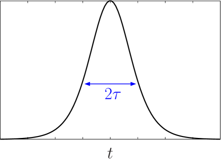
Figure 4: The temporal profile of the Sauter electrical field given in eq. (123).

The temporal profile of this field is shown in the figure 4. Since the electrical field of eq. (123) vanishes exponentially at $t\to\pm\infty$, a proper particle definition is available without any ambiguity at asymptotic times. Under the influence of this electrical field, the Dirac equation is analytically solvable [51], and one can compute the spectrum in closed form:

$$\frac{(2\pi)^{3}}{V}\;\frac{dN}{d^{3}{\bm{p}}}=\frac{\sinh\left[\pi(\lambda+\mu-\nu)\right]\sinh\left[\pi(\lambda-\mu+\nu)\right]}{\sinh\left(2\pi\mu\right)\sinh\left(2\pi\nu\right)}\;,$$ (124)

where we have defined

$$\mu\equiv\frac{\tau}{2}\sqrt{m^{2}+p_{\perp}^{2}+(p_{z}-2eE\tau)^{2}}\;,$$ (125)

$$\nu\equiv\frac{\tau}{2}\sqrt{m^{2}+p_{\perp}^{2}+p_{z}^{2}}\;,$$ (126)

$$\lambda\equiv eE\tau^{2}\;.$$ (127)

Note that ${\bm{p}}$ in these equations is the physical kinetic momentum, while in some works the spectrum is given in terms of a gauge-dependent canonical momentum.

In the figure 5, the spectrum of eq. (124) is plotted as a function of $p_{z}$, for a fixed transverse mass $\sqrt{{(m^{2}+p_{\perp}^{2})}/eE}=0.1$, and for various values of $\tau$. The spectrum has a width of order $2eE\tau$ in the $p_{z}$ direction. This can be understood as follows: particles are produced with a nearly zero momentum because the spatially homogeneous electrical field carries no momentum. After being produced, they are accelerated by the electrical field following the classical equation of motion $p_{z}=\int^{t}eE_{z}(t^{\prime})dt^{\prime}\simeq eEt$. Since the particle production and the acceleration mostly happen in the time interval $t\in[-\tau,+\tau]$, most of the particles are distributed in the range $p_{z}\in[0,2eE\tau]$.

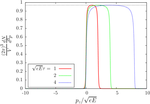
Figure 5: The spectrum (124) as a function of $p_{z}$ for various values of $\tau$. The transverse mass is fixed to $m_{\perp}/\sqrt{eE}=0.1$. A thin black horizontal line denotes $\exp(-{\pi m_{\perp}^{2}}/{(eE)})$.

The figure 6 shows the $p_{z}$-spectrum for $\sqrt{eE}\tau=4$, and for various values of the transverse mass $m_{\perp}\equiv\sqrt{m^{2}+p_{\perp}^{2}}$. The factor $\exp(-{\pi m_{\perp}^{2}}/{(eE)})$ is also indicated by thin black lines, which shows that the peak value of the spectrum agrees well with this exponential factor. In this range of parameters, the exponential $m_{\perp}$-dependence of the spectrum indicates that the particle production is dominated by the non-perturbative Schwinger effect. As we will discuss in the section 7.1, there is another range of parameters where the perturbative particle production is the dominant one.

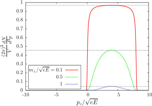
Figure 6: The spectrum (124) as a function of $p_{z}$ for various values of $m_{\perp}$. The pulse duration is fixed to $\sqrt{eE}\tau=4$. Thin black horizontal lines denote $\exp(-{\pi m_{\perp}^{2}}/{(eE)})$.

4.2 Quantum kinetic equation

In the previous subsection, we have shown that the particle spectrum can be expressed in terms of the Bogoliubov coefficients, which can be computed by solving the Dirac equation for the mode functions. When the electrical field is uniform, it is possible to derive equations that directly describe the evolution of the Bogoliubov coefficient [59]. Furthermore, if the direction of the electrical field is time-independent, one can derive an equation for the distribution function, which is called quantum kinetic equation [60, 61, 62].

Let us derive first the equations for the Bogoliubov coefficients in the presence of an uniform and time-dependent gauge field (113), whose direction may vary in time. The Bogoliubov coefficients are given by eqs. (118) and (119). Note that the momentum ${\bm{p}}$ appearing in these equations is the kinetic momentum, which is related to the canonical momentum ${\bm{q}}$ by

$${\bm{p}}={\bm{q}}-e{\bm{A}}\;.$$ (128)

Under the influence of a spatially uniform gauge field such as (113), the canonical momentum is a constant of motion, while the kinetic momentum depends on time due to the acceleration by the electrical field. When we take the time derivative of the Bogoliubov coefficients, the kinetic momentum ${\bm{p}}$ must be regarded as a time dependent quantity such that $\frac{\partial{\bm{p}}}{\partial t}=e{\bm{E}}$. In order to simplify the notations, let us treat the Bogoliubov coefficients as a $2\times 2$ matrix whose indices are the spin indexes $(s,s^{\prime})$. By taking the time derivative of the Bogoliubov coefficients given in eqs. (118) and (119), one can derive

$$\frac{d\alpha(t;{\bm{p}})}{dt}=i\,\left[\epsilon(t)+S(t)\right]\;\alpha(t;{\bm{p}})-e^{2iE_{\bm{p}}t}\;P(t)\;\beta^{*}(t;{\bm{p}})\;,$$ (129)

and

$$\frac{d\beta(t;{\bm{p}})}{dt}=i\,\left[\epsilon(t)+S(t)\right]\;\beta(t;{\bm{p}})+e^{2iE_{\bm{p}}t}\;P(t)\;\alpha^{*}(t;{\bm{p}})\;,$$ (130)

where we have defined

$$\epsilon(t)\equiv\frac{e{\bm{E}}\!\cdot\!{\bm{p}}}{E_{\bm{p}}}\;t\;,$$ (131)

$$P(t)\equiv\frac{eE_{z}E_{\bm{p}}^{2}-(e{\bm{E}}\!\cdot\!{\bm{p}})\,p_{z}}{2E_{\bm{p}}^{2}m_{\perp}}\;{\bm{1}}+i\,\frac{eE_{x}p_{y}-eE_{y}p_{x}}{2E_{\bm{p}}m_{\perp}}\;{\bm{\sigma}}^{3}+i\,\frac{m}{2E_{\bm{p}}m_{\perp}}(eE_{x}\,{\bm{\sigma}}^{2}+eE_{y}\,{\bm{\sigma}}^{1})\;,$$ (132)

and

$$S(t)\equiv\frac{m(eE_{x}\,{\bm{\sigma}}^{2}+eE_{y}\,{\bm{\sigma}}^{1})}{2E_{\bm{p}}(E_{\bm{p}}-p_{z})}+\frac{(eE_{x}p_{y}-eE_{y}p_{x})\,{\bm{\sigma}}^{3}}{2E_{\bm{p}}(E_{\bm{p}}-p_{z})}\;.$$ (133)

(The ${\bm{\sigma}}^{i}$ are the Pauli matrices.) The matrix $S(t)$ represents the precession of the spin in the electrical field, while the matrix $P(t)$ describes the rate of mixing between the coefficients $\alpha$ and $\beta$, which is closely related to the rate of pair production. The detailed form of $P(t)$ and $S(t)$ depends on the choice of a spin basis. Here we have used the free spinors whose spin basis diagonalizes the interaction with a uniform electrical field along the $z$-direction. If instead we use spinors whose spin basis is given by the eigenstates of ${\bm{\sigma}}^{3}$ in the rest frame, the form of these equations becomes essentially equivalent to those in ref. [59]. Of course, spin-averaged observables do not depend on the choice of the spin basis.

Let us now restrict ourselves to the case where the direction of the electrical field is fixed to be the $z$-direction, and derive the kinetic equation for the distribution function. In this case, the matrices $P(t)$ and $S(t)$ receive important simplifications, namely $P(t)$ is proportional to the unit matrix and $S(t)=0$. Consequently the Bogoliubov coefficients are also proportional to the unit matrix. By taking the time derivative of the distribution function (occupation number) defined by

$$f_{\bm{p}}(t)\equiv\frac{(2\pi)^{3}}{V}\;\frac{1}{2}\sum_{s}\frac{dN_{s}}{d^{3}{\bm{p}}}=\left|\beta(t,{\bm{p}})\right|^{2}\;,$$ (134)

one obtains

$$\frac{d\,f_{\bm{p}}(t)}{dt}=\frac{eE_{z}m_{\perp}}{E_{\bm{p}}^{2}}\;{\rm Re}\,(g_{\bm{p}}(t))\;,$$ (135)

where we have introduced the anomalous distribution:

$$g_{\bm{p}}(t)\equiv e^{-2iE_{\bm{p}}t}\;\alpha(t,{\bm{p}})\beta(t,{\bm{p}})\;.$$ (136)

Eq. (135) must be supplemented by an equation for the anomalous distribution,

$$\frac{d\,g_{\bm{p}}(t)}{dt}=-2iE_{\bm{p}}\;g_{\bm{p}}(t)+\frac{eE_{z}m_{\perp}}{2E_{\bm{p}}}\;\left[1-2\,f_{\bm{p}}(t)\right]\;.$$ (137)

The latter equation admits the following formal solution

$$g_{\bm{p}}(t)=\int^{t}dt^{\prime}\;\frac{eE_{z}(t^{\prime})m_{\perp}}{2E_{\bm{p}}^{2}(t^{\prime})}\;\left[1-2\,f_{\bm{p}}(t^{\prime})\right]\;e^{-i(\theta(t)-\theta(t^{\prime}))}\;,$$ (138)

where we denote

$$\theta(t)\equiv 2\int^{t}d\tau\;E_{\bm{p}}(\tau)\;.$$ (139)

The factor $1-2\,f_{\bm{p}}(t^{\prime})$ encodes the effect of Pauli blocking. By substituting eq. (138) into eq. (135), we obtain a closed equation for the distribution function itself,

$$\frac{d\,f_{\bm{p}}(t)}{dt}=\frac{eE_{z}(t)m_{\perp}}{2E_{\bm{p}}^{2}(t)}\int^{t}dt^{\prime}\;\frac{eE_{z}(t^{\prime})m_{\perp}}{E_{\bm{p}}^{2}(t^{\prime})}\;\left[1-2\,f_{\bm{p}}(t^{\prime})\right]\,\cos\left(\theta(t)-\theta(t^{\prime})\right)\;.$$ (140)

This equation is called quantum kinetic equation [60, 61, 62]. From its derivation, it should be obvious that this formalism is equivalent to solving the Dirac equation for the mode functions, as long as the background electrical field is uniform and its direction is fixed. For practical purposes in numerical calculations, it is easier to solve eqs. (135) and (137) as associated equations rather than eq. (140) which is non-local in time. The non-locality in time of eq. (140), obtained after eliminating $g_{\bm{p}}(t)$ to get a closed equation for $f_{\bm{p}}(t)$, is reminiscent of the quantum nature of the process under consideration. Similar equations to eqs. (135) and (137) for the particle production by parametric resonance in a $\phi^{4}$ scalar theory can be found in ref. [63]. In this seemingly unrelated problem, the large zero mode of the field acts as a time dependent background field for the non-zero modes. Because of this analogy, this problem is amenable to a treatment which is very similar to that of the Schwinger mechanism.

4.3 Wigner formalism

The Wigner formalism is another approach which has been applied to studies of particle production by the Schwinger mechanism [64, 65, 66, 67, 68, 69]. This approach shares the same spirit as the quantum kinetic approach in the sense that equations for one-particle distributions are obtained instead of an equation for the elementary fields, though it is more general than the quantum kinetic approach as is applicable to inhomogeneous background fields. Under the influence of inhomogeneous backgrounds, the momentum distribution function is not a well-defined quantity. Instead one can consider the Wigner function defined by

$$\mathcal{W}(t;{\bm{x}},{\bm{p}})\equiv-\frac{1}{2}\!\int\!d^{3}{\bm{s}}\,e^{-i{\bm{p}}\cdot{\bm{s}}}\;\big{<}0{}_{\rm in}\big{|}e^{-ie\int_{-1/2}^{1/2}d\lambda\,{\bm{A}}({\bm{x}}+\lambda{\bm{s}})\cdot{\bm{s}}}\,\left[\hat{\psi}(t,{\bm{x}}+{\bm{s}}/2),\overline{\hat{\psi}}(t,{\bm{x}}-{\bm{s}}/2)\right]\big{|}0{}_{\rm in}\big{>}\;.$$ (141)

A Wilson line factor is inserted between the two field operators in order to preserve the invariance under space-dependent gauge transformations (the temporal gauge condition $A^{0}=0$ is assumed). Here, we take a straight segment to connect the two points. As already mentioned earlier, if the background is not a pure-gauge potential (i.e. if there are non-zero electrical or magnetic fields), the Wilson line depends on the path one chooses. Therefore, one should keep in mind that a certain amount of arbitrariness is present here (but nothing worse than our earlier attempts to define a particle spectrum in a non-pure gauge background).

Note that since the uncertainty principle does not allow the simultaneous measurement of the position and momentum of a particle, the Wigner distribution $\mathcal{W}(t;{\bm{x}},{\bm{p}})$ is not a proper probability distribution. But its integrals over ${\bm{x}}$ or ${\bm{p}}$ are probability distributions in ${\bm{p}}$ or ${\bm{x}}$, respectively. In fact, even the positivity of the Wigner function is not guaranteed. However, it is generally the case that the support in phase-space of the negative values of $\mathcal{W}$ is of order $\hbar$. After a coarse graining of phase-space into cells of size $\hbar$ or more, these negative regions usually disappear and a probabilistic interpretation becomes plausible.

From the Dirac equation for the fermion field operator, one can derive an evolution equation for the Wigner distribution. If the gauge field is a quantum field operator, the equation is not closed and it depends on higher order correlation functions. Since here we regard the gauge field as a classical background field, a closed equation can be derived:

$$D_{t}\mathcal{W}=-\frac{1}{2}{\bm{D}}_{\bm{x}}\!\cdot\!\left[\gamma^{0}{\bm{\gamma}},\mathcal{W}\right]-im\left[\gamma^{0},\mathcal{W}\right]-i{\bm{P}}\!\cdot\!\left\{\gamma^{0}{\bm{\gamma}},\mathcal{W}\right\}\;,$$ (142)

where $D_{t}$, ${\bm{D}}_{\bm{x}}$, and ${\bm{P}}$ are non-local operators defined by

$$D_{t}\equiv\partial_{t}+e\int_{-1/2}^{1/2}d\lambda\;{\bm{E}}(t,{\bm{x}}+i\lambda\nabla_{\bm{p}})\!\cdot\!\nabla_{\bm{p}}\;,$$ (143)

$${\bm{D}}_{\bm{x}}\equiv\nabla_{\bm{x}}+e\int_{-1/2}^{1/2}d\lambda\;{\bm{B}}(t,{\bm{x}}+i\lambda\nabla_{\bm{p}})\times\nabla_{\bm{p}}\;,$$ (144)

$${\bm{P}}\equiv{\bm{p}}-ie\int_{-1/2}^{1/2}d\lambda\;\lambda\;{\bm{B}}(t,{\bm{x}}+i\lambda\nabla_{\bm{p}})\times\nabla_{\bm{p}}\;.$$ (145)

Since eq. (142) is derived from the Dirac equation (80) without any approximation, this approach is equivalent to directly solving the Dirac equation (e.g. via the mode function method). An advantage of this approach over the mode function method is that eq. (142) makes gauge invariance more manifest because it depends on the electric and magnetic fields but not on the gauge field (but keep in mind the caveat mentioned in the paragraph following eq. (141)). Although eq. (142) is valid for arbitrary space-dependent electromagnetic fields, the numerical implementation of the non-local operators is difficult to achieve. Effects of a small spatial inhomogeneity have been studied with a derivative expansion in ref. [66]. When the electric field is uniform with a fixed direction and the magnetic field is absent, eq. (142) can be reduced to the quantum kinetic equation (140) [66].

5 Numerical methods on the lattice

5.1 Real-time lattice numerical computations

As discussed in the section 4.1, any observable may in principle be computed once we have obtained the mode functions $\psi_{{\bm{p}},s}^{\pm}(x)$ by solving the Dirac equation. This method is applicable to completely general space and time dependent background fields. Although we have mainly discussed the momentum spectrum of the produced particles in the previous sections, other observables like the charged current and the energy-momentum tensor can also be expressed in terms of the mode functions. For example, the vacuum expectation value of a fermion bilinear operator $\hat{\psi}^{\dagger}(x){\bm{M}}\hat{\psi}(y)$, where ${\bm{M}}$ is a matrix in the spinor and coordinate spaces, can be represented in terms of the mode functions as

$$\big{<}0{}_{\rm in}\big{|}\hat{\psi}^{\dagger}(x){\bm{M}}\hat{\psi}(y)\big{|}0{}_{\rm in}\big{>}=\sum_{s}\int\frac{d^{3}{\bm{p}}}{(2\pi)^{3}2E_{\bm{p}}}\;\psi_{{\bm{p}},s}^{\text{in}-\,\dagger}(x)\,{\bm{M}}\,\psi_{{\bm{p}},s}^{\text{in}-}(y)\;.$$ (146)

Also the momentum spectrum (109) can be expressed in this form. In the following, we will omit the index ‘in’, since the out-mode functions do not appear.

Our problem is thus reduced to solving the Dirac equation for the mode functions with the initial condition (85). For general space and time dependent background fields, it is impossible to solve the Dirac equation analytically, and we therefore need to resort to numerical computations. In this subsection, we briefly explain a possible lattice setup for this numerical implementation in SU($N_{c}$) gauge theory [70, 71]. We assume the temporal gauge condition $A^{0}=0$, and treat the time variable $t$ as a continuum variable. We divide the 3-dimensional volume, that we take of size of $L_{x}\times L_{y}\times L_{z}$, into $N_{x}\times N_{y}\times N_{z}$ lattice sites. The space coordinates are labeled by integers $n_{i}$ $(i=x,y,z)$ as follows

$$(x,y,z)=(n_{x}a_{x},n_{y}a_{y},n_{z}a_{z})\;,$$ (147)

where the numbers $a_{i}=L_{i}/N_{i}$ are the lattice spacings. It is common practice to use periodic boundary condition (in space) for the fields.

On the lattice, it is more convenient to consider the link variables

$$\mathcal{U}_{i}(x)\equiv e^{ia_{i}gA_{i}(x)}\;,$$ (148)

that are Wilson lines spanning one elementary edge of the lattice, as the fundamental variables, instead of the gauge fields $A_{i}(x)$. After the gauge fixing by the temporal gauge condition, there is a residual invariance under gauge transformations that depend only on the spatial coordinates. It is highly desirable to preserve exactly this residual invariance through the discretization. Under such a gauge transformation, the fermion fields and the link variables are transformed as

$$\psi(t,{\bm{x}})\longrightarrow\Omega({\bm{x}})\;\psi(t,{\bm{x}})\;,$$ (149)

and

$$\mathcal{U}_{i}(t,{\bm{x}})\longrightarrow\Omega({\bm{x}})\;\mathcal{U}_{i}(t,{\bm{x}})\;\Omega^{\dagger}({\bm{x}}+\hat{i})\;.$$ (150)

Therefore, a natural definition for the covariant derivative applied to the fermion field reads

$$D_{i}\psi(x)\equiv\frac{1}{2a_{i}}\left[\mathcal{U}_{i}(x)\;\psi(x+\hat{i})-\mathcal{U}_{i}^{\dagger}(x-\hat{i})\;\psi(x-\hat{i})\right]\;,$$ (151)

where we have used a centered difference in order to preserve the unitarity of the theory. This covariant derivative transforms as expected under the residual gauge transformations. With this definition, the Dirac equation on the lattice reads

$$\left[i\gamma^{0}\partial_{0}+i\gamma^{i}D_{i}-m\right]\psi(x)=0\;.$$ (152)

If we regard the background gauge fields as generated from some given sources, we need to solve the Yang-Mills equations on the lattice in addition to the Dirac equation. The lattice Yang-Mills equation can be derived from the lattice Hamiltonian for the SU($N_{c}$) gauge fields,

$$\mathcal{H}_{\text{gauge}}=\sum_{i=1}^{3}{\rm tr}\,\big{(}E_{i}E_{i}\big{)}+\frac{N_{c}}{g^{2}}\underset{(j\neq i)}{\sum_{j=1}^{3}}\frac{1}{a_{i}^{2}a_{j}^{2}}\left\{1-\frac{1}{N_{c}}{\rm Re}\,\left[{\rm tr}\,\big{(}\mathcal{U}_{i,j}(x)\big{)}\right]\right\}\;,$$ (153)

where the $E_{i}(x)$ are the electrical fields, and the variables $\mathcal{U}_{ij}(x)$, called plaquettes, are defined by

$$\mathcal{U}_{i,j}(x)\equiv U_{i}(x)\,U_{j}(x+\hat{i})\,U_{i}^{\dagger}(x+\hat{j})\,U_{j}^{\dagger}(x)\;.$$ (154)

(Plaquettes are Wilson loops spanning an elementary square on the lattice.) The Hamilton equations then read

$$\partial_{t}\,\mathcal{U}_{i}(x)=iga_{i}\,E_{i}(x)\;\mathcal{U}_{i}(x)\;,$$ (155)

and

$$\partial_{t}\,E_{i}(x)=-\frac{1}{g\,a_{i}}\underset{(j\neq i)}{\sum_{j=1}^{3}}\frac{1}{a_{j}^{2}}\;{\rm Im}\,\left[\,\mathcal{U}_{i,j}(x)+\mathcal{U}_{i,-j}(x)\right]-\text{(trace)}\;,$$ (156)

where

$$\mathcal{U}_{i,-j}(x)\equiv\mathcal{U}_{i}(x)\,\mathcal{U}_{j}^{\dagger}(x+\hat{i}-\hat{j})\,\mathcal{U}_{i}^{\dagger}(x-\hat{j})\,\mathcal{U}_{j}(x-\hat{j})$$ (157)

and where, for an element $X$ of the fundamental representation of the SU($N_{c}$) algebra, the notation “$X-$(trace)” means

$$X-\text{(trace)}=X-\frac{1}{N_{c}}\,{\rm tr}\,\big{(}X\big{)}\;.$$ (158)

For a U(1) theory such as QED, the $-$(trace) term must of course be ignored.

Because we employ the centered difference in eq. (151), the lattice momentum for the fermion fields suffers from the problem of doublers. In $d$-dimensional momentum space, there is a $2^{d}$-fold degeneracy. If the background field is spatially homogeneous, it does not carry any nonzero momenta. Therefore, fermions in different momentum modes do not interact with each other, and thus all these degenerated modes remain independent. In this case, we can simply eliminate the effect of the doublers by dividing expectation values by the number of degenerated modes, as long as all the degenerated modes contribute to the expectation value equally. However, when the background gauge field is inhomogeneous, it carries nonzero momenta that cause interactions between fermions in different momentum modes. In this case, a non-trivial mixing happens between degenerate doubler modes, and the fermionic observables may be contaminated by the doublers. One way to suppress the doubler modes is to add the Wilson term to the Dirac equation, which now reads

$$\left(i\gamma^{0}\partial_{0}+i\gamma^{i}D_{i}-m\right)\psi(x)+\frac{r}{2}\sum_{i=1}^{3}\frac{1}{a_{i}}\left[\mathcal{U}_{i}(x)\,\psi(x+\hat{i})-2\psi(x)+\mathcal{U}_{i}^{\dagger}(x-\hat{i})\,\psi(x-\hat{i})\right]=0\;,$$ (159)

where $r$ is a positive parameter. Thanks to the addition of the Wilson term, the doubler modes acquire a heavy mass of the order of the lattice ultraviolet cutoff $1/a$, and therefore they decouple from the dynamics when $a\to 0$. Note that the numerical results presented in the subsections 5.3 and 7.2 are computed without the Wilson term since the background gauge fields considered there are uniform.

5.2 Statistical sampling method

5.2.1 Formulation

In the previous subsection, we have presented a lattice formulation of the Dirac and Yang-Mills equations. Each mode function $\psi_{{\bm{p}},s}^{\pm}(x)$ obeys the Dirac equation

$$\left[i\gamma^{0}\partial_{0}+i\gamma^{i}D_{i}-m\right]\psi_{{\bm{p}},s}^{\pm}(x)=0\;.$$ (160)

This equation must be solved for each momentum modes (and other quantum numbers as well). Therefore, the numerical cost to solve the equation is proportional to $N_{\text{latt}}^{2}N_{t}$, where $N_{\text{latt}}\equiv N_{x}N_{y}N_{z}$ is the number of lattice sites and $N_{t}$ is the number of time steps. This cost has a very unfavorable scaling with the size of the lattice, especially in 3 dimensional space. If the system has some spatial symmetry, this rather expensive cost can be reduced. For instance, if the system is completely uniform, the ${\bm{x}}$-dependence of the mode functions is analytically known to be $e^{i{\bm{p}}\cdot{\bm{x}}}$. In this case, we do not need to treat the space-dependence of the field numerically, and thus the cost is reduced to $N_{\text{latt}}N_{t}$.

In the absence of any such symmetries, a way to reduce the numerical cost is to replace the exhaustive listing of the momentum modes by a Monte Carlo sampling method, which is applicable to any space and time dependent background. However, instead of picking randomly a subset of the set of momenta, one can exploit the linearity of the Dirac equation and use random spinors that are linear superpositions (with random coefficients) of all the momentum modes [72, 49]. This approach provides a better sampling of the entire momentum space.

Let us introduce a stochastic field which is a linear superposition of the mode functions with random number coefficients:

$$\psi_{c}^{-}(x)=\frac{1}{\sqrt{V}}\sum_{{\bm{k}},s}\frac{1}{\sqrt{2E_{\bm{k}}}}\;c_{{\bm{k}},s}\;\psi_{{\bm{k}},s}^{-}(x)\;,$$ (161)

where the random numbers are Gaussian distributed with zero mean value and the following variance:

$$\langle c_{{\bm{k}},s}c_{{\bm{k}}^{\prime},s^{\prime}}^{*}\rangle_{\text{ens}}=\delta_{{\bm{k}},{\bm{k}}^{\prime}}\delta_{s,s^{\prime}}\;.$$ (162)

$\langle\cdots\rangle_{\text{ens}}$ denotes the ensemble average over these random numbers. Using this stochastic field, we can express the expectation value of a bilinear operator (146) as follows:

$$\big{<}0{}_{\rm in}\big{|}\hat{\psi}^{\dagger}(x)\,{\bm{M}}\,\hat{\psi}(y)\big{|}0{}_{\rm in}\big{>}=\langle\psi_{c}^{-\,\dagger}(x)\,{\bm{M}}\,\psi_{c}^{-}(y)\rangle_{\text{ens}}\;.$$ (163)

Because the Dirac equation is linear, the stochastic fields (161) obey the same Dirac equation as the mode functions. Therefore, expectation values at time $t$ can be computed by the following procedure:

• At an initial time $t=t_{0}$, draw random numbers following the variance (162), and compute a stochastic field (161) by using the initial value for the mode functions $\psi_{{\bm{p}},s}^{-}(t_{0},{\bm{x}})$. In most practical cases, the mode functions at $t_{0}$ are known analytically.

• Solve the Dirac equation for the stochastic field until the time $t$, and compute the contribution of this field to the observable.

• Repeat the steps i and ii in to perform the ensemble average until satisfactory statistical errors are reached.

The numerical cost of the step i is proportional to $N_{\text{latt}}^{2}$ since the sum over the momentum modes must be done at each spatial coordinate. This cost scales unfavorably with $N_{\text{latt}}$. However, this must be computed only at the initial time. The cost for the time evolution is lower than that of the direct mode function method, since it is proportional to $N_{\text{latt}}N_{t}$ for each configuration of the stochastic field. If we compute $N_{\text{conf}}$ configurations for the stochastic field, the total cost is roughly proportional to $(N_{\text{latt}}^{2}+N_{\text{latt}}N_{t})N_{\text{conf}}$. This cost is lower than that of the direct mode function method provided that

$$N_{\text{conf}}\ll N_{\text{latt}}\quad\text{and}\quad N_{\text{conf}}\ll N_{t}\;,$$

both of which are easily satisfied in practice.

5.2.2 Statistical errors

Eq. (163) is exact only if the number of configurations $N_{\text{conf}}$ is infinite. In practice, we have to use a finite $N_{\text{conf}}$, which implies nonzero statistical errors. In this subsection, we describe a method to evaluate the statistical errors [49]. We consider the following vacuum expectation:

$$\big{<}0{}_{\rm in}\big{|}\hat{\mathcal{O}}\big{|}0{}_{\rm in}\big{>}\equiv\sum_{X,f}\big{<}0{}_{\rm in}\big{|}\hat{\psi}^{\dagger}(x)\,{\bm{M}}\,\hat{\psi}(y)\big{|}0{}_{\rm in}\big{>}\;,$$ (164)

where the sum over $X$ denotes possible summation over $x$ and $y$ coordinates (for instance in a Fourier transform to compute a spectrum), and the sum over $f$ is over some other quantum numbers that the matrix ${\bm{M}}$ may carry. For instance, in the case of the momentum spectrum (109), the matrix ${\bm{M}}$ is

$${\bm{M}}_{\text{spec}}=\frac{1}{(2\pi)^{3}2E_{\bm{p}}}\;u({\bm{p}},s)u^{\dagger}({\bm{p}},s)\;U^{\dagger}(t,{\bm{x}})\,U(t,{\bm{y}})\;e^{-i{\bm{p}}\cdot({\bm{x}}-{\bm{y}})}\;,$$ (165)

and $X$ stands for $\{{\bm{x}},{\bm{y}}\}$. If we compute the spin-averaged spectrum, $f$ would be the final spin $s$.

With a finite number $N_{\text{conf}}$ of configurations, the statistical evaluation of the expectation value (164) can be expressed as

$$\mathcal{O}_{N_{\text{conf}}}=\frac{1}{V}\sum_{X,f}\sum_{J,J^{\prime}}\frac{1}{2\sqrt{E_{J}E_{J^{\prime}}}}\;C_{N_{\text{conf}}}(J,J^{\prime})\;\psi_{J}^{-\,\dagger}(x)\,{\bm{M}}\,\psi_{J^{\prime}}^{-}(y)\;\;,$$ (166)

where $J$ is a shorthand notation for $({\bm{k}},s)$. The coefficient $C_{N_{\text{conf}}}$ contains the average over $N_{\text{conf}}$ samples of the Gaussian random numbers $c_{J}^{(n)}$:

$$C_{N_{\text{conf}}}(J,J^{\prime})\equiv\frac{1}{N_{\text{conf}}}\sum_{n=1}^{N_{\text{conf}}}c_{J}^{(n)*}c_{J^{\prime}}^{(n)}\;.$$ (167)

$C_{N_{\text{conf}}}$ itself is a random number, whose fluctuations determine the statistical error of the evaluation (166). From the variance of the random coefficients $c^{(n)}_{J}$, we obtain immediately the following mean value for $C_{N_{\text{conf}}}(J,J^{\prime})$

$$\langle C_{N_{\text{conf}}}(J,J^{\prime})\rangle=\delta_{J,J^{\prime}}\;.$$ (168)

Furthermore, if we assume for simplicity that the $c_{J}^{(n)}$ are Gaussian distributed (with no correlations if $n\not=n^{\prime}$), we obtain the following variance

$$\langle C_{N_{\text{conf}}}(J,J^{\prime})C_{N_{\text{conf}}}(K,K^{\prime})\rangle-\langle C_{N_{\text{conf}}}(J,J^{\prime})\rangle\langle C_{N_{\text{conf}}}(K,K^{\prime})\rangle=\frac{1}{N_{\text{conf}}}\delta_{J,K^{\prime}}\delta_{K,J^{\prime}}\;,$$ (169)

which decreases as one increases the number of configurations. By using this equation, we can compute the variance of the statistical evaluation (166) by

$$\begin{split}\langle\mathcal{O}_{N_{\text{conf}}}^{2}\rangle-\langle\mathcal{O}_{N_{\text{conf}}}\rangle^{2}=\frac{1}{N_{\text{conf}}}\frac{1}{V^{2}}\sum_{J,J^{\prime}}\frac{1}{4E_{J}E_{J^{\prime}}}\;\Big{|}\sum_{X,f}\psi_{J}^{-\,\dagger}(x)\,{\bm{M}}\,\psi_{J^{\prime}}^{-}(y)\Big{|}^{2}\;.\end{split}$$ (170)

The square root of the right hand side provides an estimate of the statistical error. We can compute it by the statistical method in the following procedure:

• Prepare two stochastic fields

  $$\psi_{1,2}^{-}(x)=\frac{1}{\sqrt{V}}\sum_{J}\frac{1}{\sqrt{2E_{J}}}\;c_{J}^{(1,2)}\,\psi_{J}^{-}(x)\;,$$ (171)

  with uncorrelated random numbers $c_{J}^{(1)}$ and $c_{J}^{(2)}$.

• Evolve these two stochastic fields by solving their Dirac equation.

• Compute

  $$\Big{|}\sum_{X,f}\psi_{1}^{-\,\dagger}(x)\,{\bm{M}}\,\psi_{2}^{-}(y)\Big{|}^{2}\;.$$ (172)

• Repeat the steps i-iii in order to average over the random numbers $c_{J}^{(1)}$ and $c_{J}^{(2)}$. Because this is merely for an error estimate, one does not need a large number of samples.

• At the last step, take the square root and divide the result by $\sqrt{N_{\text{conf}}}$.

Since the summand of the sum over $X,f$ in eq. (170) is generally a complex number, phase cancellations may happen in the summation over $X$ and $f$, making the statistical error smaller. For example, the transverse spectrum, which is obtained by summing over $f\equiv(p_{z},s)$, should contain smaller statistical error compared with the full momentum spectrum that depends on $p_{z}$ and ${\bm{p}}_{\perp}$.

5.2.3 Relation to the low-cost fermion method

In real-time lattice simulations for fermion fields, another method called the low-cost fermion method [73] has been used in several works [74, 75, 76, 77]. In the low-cost fermion method, instead of using one stochastic field (161), one employs two kinds of stochastic fields called “male” and “female” fields:

$$\psi_{\text{M}}(x) \equiv\frac{1}{\sqrt{2V}}\sum_{{\bm{k}},s}\frac{1}{\sqrt{2E_{\bm{k}}}}\;\left[c_{{\bm{k}},s}\,\psi_{{\bm{k}},s}^{+}(x)+d_{{\bm{k}},s}\,\psi_{{\bm{k}},s}^{-}(x)\right]\;,$$ (173)

$$\psi_{\text{F}}(x) \equiv\frac{1}{\sqrt{2V}}\sum_{{\bm{k}},s}\frac{1}{\sqrt{2E_{\bm{k}}}}\;\left[c_{{\bm{k}},s}\,\psi_{{\bm{k}},s}^{+}(x)-d_{{\bm{k}},s}\,\psi_{{\bm{k}},s}^{-}(x)\right]\;,$$ (174)

where $c_{{\bm{k}},s}$ and $d_{{\bm{k}},s}$ are independent random numbers which have the same variance as (162). Combining these two fields, one can obtain the vacuum expectation value of a symmetrized bilinear operator by an ensemble average as follows:

$$\begin{split}\big{<}0{}_{\rm in}\big{|}\frac{1}{2}\left[\hat{\psi}^{\dagger}(x),{\bm{M}}\,\hat{\psi}(y)\right]\big{|}0{}_{\rm in}\big{>}&=\frac{1}{2V}\sum_{{\bm{k}},s}\frac{1}{2E_{\bm{k}}}\;\left[\psi_{{\bm{k}},s}^{-\,\dagger}(x)\,{\bm{M}}\,\psi_{{\bm{k}},s}^{-}(y)-\psi_{{\bm{k}},s}^{+\,\dagger}(x)\,{\bm{M}}\,\psi_{{\bm{k}},s}^{+}(y)\right]\\ &=-\big{<}\psi_{\text{M}}^{\dagger}(x)\,{\bm{M}}\,\psi_{\text{F}}(y)\big{>}_{\text{ens}}\;.\end{split}$$ (175)

The two kinds of fields are necessary in order to obtain the minus sign in front of the second term in the right hand side of the first line, which originates from the anti-commutation relation for the fermionic operators. For bosonic fields, one would need only one kind of stochastic field [72].

By using the completeness relation

$$\frac{1}{V}\sum_{{\bm{k}},s}\frac{1}{2E_{\bm{k}}}\;\left[\psi_{{\bm{k}},s}^{+}(t,{\bm{x}})\psi_{{\bm{k}},s}^{+\,\dagger}(t,{\bm{y}})+\psi_{{\bm{k}},s}^{-}(t,{\bm{x}})\psi_{{\bm{k}},s}^{-\,\dagger}(t,{\bm{y}})\right]=V\,\delta_{{\bm{x}},{\bm{y}}}\,\mbox{1}\mbox{l}$$ (176)

(1l is the unit matrix in the spinor space), we can relate the quantities evaluated in the simple statistical method (163) and that in the low-cost fermion method (175) by

$$\big{<}\psi_{c}^{-\,\dagger}(x)\,{\bm{M}}\,\psi_{c}^{-}(y)\big{>}_{\text{ens}}=-\big{<}\psi_{\text{M}}^{\dagger}(x)\,{\bm{M}}\,\psi_{\text{F}}(y)\big{>}_{\text{ens}}+\frac{V}{2}\;\text{tr}\,\left({\bm{M}}\,\delta_{{\bm{x}},{\bm{y}}}\right)\;.$$ (177)

Therefore, the two methods provide the same result for the vacuum expectation value up to a zero-point vacuum contribution. However, the method (163) has an advantage over the low-cost fermion method: it leads to smaller statistical errors for the evaluation of the spectrum if the value of the spectrum is much smaller than one. In the statistical method (163), the spectrum is directly obtained by the statistical ensemble. On the other hand, in the low-cost fermion method (175), one gets instead a direct access to $\frac{1}{2}-f_{\bm{p}}$ ($f_{\bm{p}}$ being the fermion occupation number), and the zero-point occupation number 1/2 must be subtracted. Because this vacuum 1/2 also contains statistical errors, the low-cost fermion method suffers from relatively larger statistical errors when the occupation number is much smaller than 1/2.

5.3 Numerical example

To demonstrate the efficiency of the statistical method, we use it in order to compute the momentum spectrum of particles produced in the Sauter electrical field (123). For this background field, one can use the analytic expression (124) to monitor the accuracy of the numerical evaluation. In the figure 7, the $p_{z}$-spectrum computed by the statistical method based on eq. (161) is compared with the analytical result. The lattice parameters used for this computation are $N_{x}=N_{y}=48$, $N_{z}=128$, $\sqrt{eE}\,a_{x}=\sqrt{eE}\,a_{y}=0.42$, $\sqrt{eE}\,a_{z}=0.16$, and $N_{\text{conf}}=256$. The statistical errors evaluated by the formula (170) are indicated by error bars. As shown in this plot, the evaluation by the statistical method is in good agreement with the exact results.

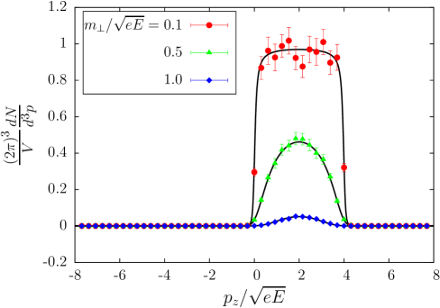
Figure 7: Comparison of the spectrum computed by the statistical method and the analytic result (black lines) in the Sauter electrical field with $\sqrt{eE}\tau=2$. This plot shows the $p_{z}$-spectra for fixed values of $m_{\perp}$. The lattice parameters are $N_{z}=128$, $\sqrt{eE}a_{z}=0.16$, and $N_{\text{conf}}=256$.

In the figure 8, the spectrum computed by the statistical method (161) is compared to the result of the low-cost fermion method (175). Firstly, we see that both methods agree well with the exact result. As we have pointed out in the section 5.2.3, the statistical errors for the single-field stochastic method are smaller than those of the male-female method in the region where the spectrum is smaller than 1/2. This difference becomes crucial when we compute the particle production in the weak field (or high momentum) regime such that $eE<m_{\perp}^{2}$. In such weak fields, the occupation number of produced particle is much smaller than one. In order to resolve these small occupation numbers, we need to ensure that the statistical errors are smaller than the occupation number itself. This is easily attainable if we use the single stochastic field method. In the figure 9, we display the spectrum computed by the single stochastic field method in a weak field $eE=0.25\,m^{2}$, $\sqrt{eE}\,\tau=25.5$. The lattice parameters are $N_{z}=256$, $ma_{z}=0.048$, and $N_{\text{conf}}=48$. The occupation number of the order of $10^{-6}$ that one obtains with these parameters is accurately reproduced within statistical errors. If one had used the male-female method, an extremely large number of configurations of the order of $10^{12}$ would have been necessary in order to achieve a similar statistical accuracy, because large statistical errors arise from the vacuum $1/2$.

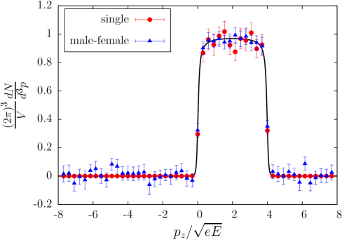
Figure 8: Comparison of the two statistical methods; one using the single kind of stochastic field (161) and the other using the male-female fields (175). $\sqrt{eE}\,\tau=2$ and $m_{\perp}/\sqrt{eE}=0.1$. The lattice parameters are the same as those in the figure 7.

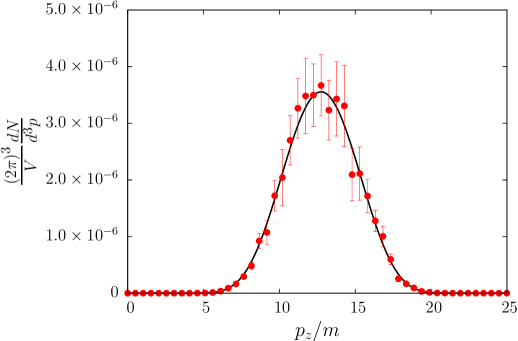
Figure 9: Comparison of the spectra computed by the statistical method and the analytic result (black line) in a weak field regime, $eE=0.25\,m^{2}$, $\sqrt{eE}\,\tau=25.5$. The lattice parameters are $N_{z}=256$, $ma_{z}=0.048$, and $N_{\text{conf}}=48$.

5.4 Back reaction

In the previous subsection, we have shown the momentum spectra of particles produced in a gauge field whose evolution is controlled by a given external current. At the level of accuracy at which this calculation was done, the total energy of the system (the electromagnetic field and the produced particles) is not conserved. In order to conserve the total energy, we must take into account the back reaction of the produced particles on the gauge field. When a particle-antiparticle pair is produced, the gauge field is weakened because it looses the energy that the pair takes away and eventually decays [78, 79]. In other words, when a particle-antiparticle pair is produced, the background gauge field is screened by the produced charges. This screening effect is crucial for the description of string breaking in the color flux tube model [80, 81, 82]. In addition to static charges, the screening can also be caused by moving charges (conduction current) [7]. These effects can be taken into account if the gauge field is coupled to a current induced the by produced particles:

$$\partial_{\mu}F^{\mu\nu}(x)=\langle\hat{J}^{\nu}(x)\rangle\;,$$ (178)

where $\hat{J}^{\nu}(x)$ is charged current operator, and $\langle\cdots\rangle$ denotes the quantum expectation value by an initial state. In the case of the lattice formulation, the current must be added to the right hand side of eq. (156).

The description of the back reaction by eq. (178) can be justified in the mean field approximation based on the large-$N_{f}$ expansion [83], or by the classical-statistical approximation for strong gauge fields [77]. Numerical computations including the back reaction problem have been conducted in several studies [84, 85, 86, 87, 62, 88, 89, 90, 91, 57, 92, 93, 77].

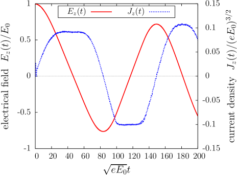
Figure 10: The time evolution of the electrical field $E_{z}(t)$ scaled by its initial value $E_{0}$ (solid line, left axis), and the induced charge current $J_{z}(t)$ divided by $(eE_{0})^{3/2}$ (dotted line, right axis). The parameters are $e=0.3$, $m/\sqrt{eE_{0}}=0.1$, $N_{x}=N_{y}=48$, $N_{z}=512$, $\sqrt{eE_{0}}\,a_{x}=\sqrt{eE_{0}}\,a_{y}=0.62$, $\sqrt{eE_{0}}\,a_{z}=0.029$.

As an illustration of the effects of back reaction, we show numerical results obtained in real-time lattice computations. We have solved (the lattice version of) the Maxwell equation (178) with a uniform electrical field, $E_{z}(0)=E_{0}$, as initial condition. For the fermionic sector, the mode functions are directly computed by solving the Dirac equation, and the charge current appearing in the right hand side of eq. (178) is calculated at every time step. The parameters used in the computation are $e=0.3$, $m/\sqrt{eE_{0}}=0.1$, $N_{x}=N_{y}=48$, $N_{z}=512$, $\sqrt{eE_{0}}\,a_{x}=\sqrt{eE_{0}}\,a_{y}=0.62$, $\sqrt{eE_{0}}\,a_{z}=0.029$. In the figure 10, the time evolution of the electrical field $E_{z}(t)$ and the induced current density $J_{z}(t)$ are shown. As particles are produced and accelerated by the electrical field, a positive charge current is induced, causing the reduction of the electrical field strength through the Maxwell equation (178). At some point ($\sqrt{eE_{0}}\,t\simeq 45$), the field strength vanishes. However, since particles are already accelerated to high momenta, the decrease of the electrical field does not stop and its direction is flipped. Then, the particles start to be accelerated in the opposite direction. The repeat of such processes results in plasma oscillations. Thanks to the back reaction, the total energy is indeed conserved (see the figure 11).

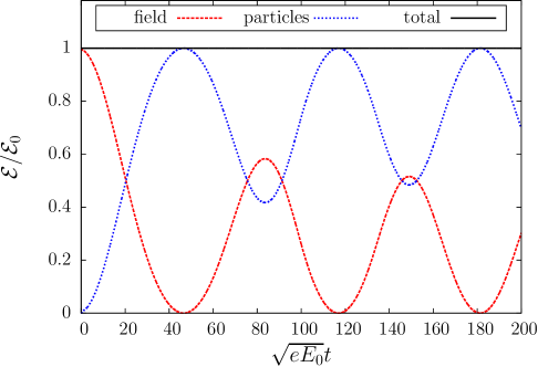
Figure 11: The time dependence of the energy density divided by $\mathcal{E}_{0}=\frac{1}{2}E_{0}^{2}$. The energy density of the electrical field and that of produced particles are individually plotted as well as total energy density.

The $p_{z}$-spectrum of produced particles is shown in the figure 12. In the top figure, the spectrum at early times before the first minimum of the electrical field happens is plotted. In this time range, the behavior of the spectrum is very similar to that obtained in the Sauter electrical field, that we have shown in the section 4.1.3: Particles are produced with a nearly zero longitudinal momentum and then accelerated by the electrical field. Their occupation number is given by $\exp(-\pi m_{\perp}^{2}/(eE))$.

After the direction of the electrical field is flipped, non-trivial quantum interference phenomena occur. Because the direction of the electrical field is negative from $\sqrt{eE_{0}}\,t\sim 60$ to $\sim 100$, the produced particles are accelerated in the negative $z$ direction, and thus the $p_{z}$-spectrum is shifted towards the negative momentum region. While doing this, they cross the zero momentum point $p_{z}=0$, where particles are still being produced by the electrical field (for a spatially homogeneous field, the particles are created at nearly zero momentum). Pauli blocking and interferences with the pre-existing particles lead to a spectrum that displays distinct features in the region $p_{z}<0$: (i) its magnitude is significantly smaller than $\exp(-\pi m_{\perp}^{2}/(eE))$ and (ii) it shows rapid oscillation in $p_{z}$ (see ref. [92]). Because of this interference phenomenon that repeats with each oscillation of the field, the spectrum at $\sqrt{eE_{0}}\,t=200$ is not smooth, in contrast to the spectrum at early times shown in the top figure. Even though this system is closed and the equations of motion are symmetric under time-reversal, an apparent irreversibility of the energy flow from coherent fields to fluctuating quantum modes emerges [94]. In the figure 11, we can indeed see that the oscillation amplitude of the electrical field is slightly decreasing in time.

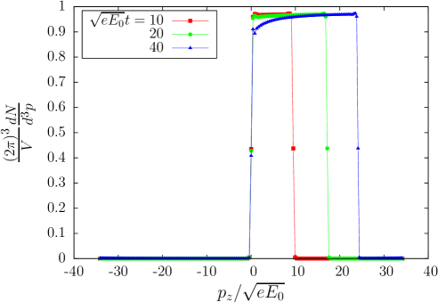
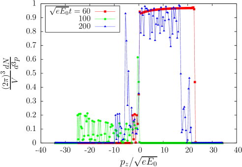
Figure 12: Plots of the $p_{z}$-spectrum with fixed transverse momentum $p_{\perp}=0$ with back reaction taken into account. The spectrum at several times is plotted (Top: early times, Bottom: later times). The parameters are the same as those in the figure 10.

6 Worldline formalism

Up to this point, our discussion of the Schwinger mechanism was following a fairly standard quantum field theoretical approach based on diagrammatic expansions and field equations of motion. The non-perturbative nature of the phenomenon resulted in the necessity of summing infinite sets of Feynman graphs, the sum of which may be re-expressed in terms of solutions of some partial differential equations (classical field equations of motion at Leading Order, or the equation of motion for the mode functions over a background field at one-loop).

In the past ten years, a radically different approach –the worldline formalism– has been applied to the study of the Schwinger mechanism. The worldline formalism first emerged from ideas around the limit of infinite string tension in string theory [95, 96, 97] but its potential for performing efficiently 1-loop calculations in quantum field theories was soon realized. This formalism was later establish of purely field theoretical grounds in ref. [98], in an approach reminiscent of Schwinger’s proper time method. Reviews on this formalism can be found in refs. [99, 100]. Its main application, of direct interest to us in this review, if the calculation of 1-loop effective actions in a background field [101, 102, 103, 104], with special emphasis on pair creation in refs. [105, 106], but is has also been used in studies of the Casimir effect [107, 108].

Although the result for the Schwinger mechanism should not depend on the method used to obtain it, the worldline formalism offers very interesting new insights about the space-time development of the particle production process, and provides completely novel numerical approaches to these calculations. In this section, we will present several aspects of the worldline approach by returning to the simple example of scalar QED in an external field for illustration purposes.

6.1 Worldline formalism for pair production

As we have discussed in the section 2, the vacuum to vacuum transition amplitude can be written as an exponential,

$$\big{<}0_{\rm out}\big{|}0{}_{\rm in}\big{>}=e^{i\,{\cal V}}\;,$$ (179)

where $i\,{\cal V}$ is the sum of all the connected vacuum diagrams. The possibility of particle production is intimately related to the imaginary part of ${\cal V}$, since the total probability of producing particles reads

$$\sum_{n=1}^{\infty}P_{n}=1-P_{0}=1-e^{-2\,{\rm Im}\,{\cal V}}\;.$$ (180)

In scalar QED, the graphs made of one scalar loop embedded in a background electromagnetic field lead to the following contribution to ${\cal V}$,

$${\cal V}_{\rm 1\ loop}=\ln\,{\rm det}\,\left(g_{\mu\nu}D^{\mu}D^{\nu}+m^{2}\right)\;,$$ (181)

where $D^{\mu}$ is the covariant derivative in the background field and $g_{\mu\nu}$ is Minkowski’s metric tensor. For technical reasons related to the definition of the worldline formalism, we should introduce the Euclidean analogue of this quantity,

$${\cal V}_{{}_{E},\rm 1\ loop}\equiv\ln\,{\rm det}\,\left(-D^{i}D^{i}+m^{2}\right)={\rm Tr}\,\ln\left(-D^{i}D^{i}+m^{2}\right)\;,$$ (182)

where the index $i$ runs over the values $1,2,3,4$ (4 being the Euclidean time). The worldline formalism can be derived from several points of view. A simple starting point is Schwinger’s proper time representation of inverse propagators,

$$\left(-D^{i}D^{i}+m^{2}\right)^{-1}=\int_{0}^{\infty}{d\tau}\;\exp\left(-\tau\big{(}-D^{i}D^{i}+m^{2}\big{)}\right)\;,$$ (183)

that leads to the following formula for the logarithm

$$\ln\left(-D^{i}D^{i}+m^{2}\right)=-\int_{0}^{\infty}\frac{d\tau}{\tau}\;\exp\left(-\tau\big{(}-D^{i}D^{i}+m^{2}\big{)}\right)\;,$$ (184)

up to some irrelevant integration constant. Using standard manipulations, the trace of the exponential can then be rewritten as a path integral over closed loops in Euclidean space-time:

$${\cal V}_{{}_{E},\rm 1\ loop}=-\int_{0}^{\infty}\frac{d\tau}{\tau}\;e^{-m^{2}\tau}\;\int\limits_{x^{i}(0)=x^{i}(\tau)}\big{[}{\cal D}x^{i}(\tau^{\prime})\big{]}\;\exp\Big{(}-\int_{0}^{\tau}d\tau^{\prime}\;\big{(}\frac{\dot{x}^{i}\dot{x}^{i}}{4}+ie\,\dot{x}^{i}A^{i}(x)\big{)}\Big{)}\;.$$ (185)

This formula involves a double integration: a path integral over all the worldlines $x^{i}(\tau^{\prime})$, i.e. closed paths in Euclidean space-time parameterized by the fictitious time $\tau^{\prime}\in[0,\tau]$, and an ordinary integral over the length $\tau$ of these paths. The dot denotes a derivative with respect to the fictitious time. The sum over all the worldlines can be viewed as a materialization of the quantum fluctuations in space-time, and the prefactor $\exp(-m^{2}\tau)$ suppresses the very long worldlines that explore regions of space-time that are much larger than the Compton wavelength of the particles (making obvious the role of the mass as an infrared regulator). In contrast, the ultraviolet properties of the theory under consideration are controlled by the short worldlines, i.e. the limit $\tau\to 0$. Note that going to Euclidean space-time was necessary in order to obtain convergent integrals in eq. (185). In the vacuum, i.e. when there is no background field, one can use the following standard result in $d$ space-time dimensions,

$$\int\limits_{x^{i}(0)=x^{i}(\tau)}\big{[}{\cal D}x^{i}(\tau^{\prime})\big{]}\;\exp\Big{(}-\int_{0}^{\tau}d\tau^{\prime}\;\frac{\dot{x}^{i}\dot{x}^{i}}{4}\Big{)}=\frac{1}{(4\pi\tau)^{d/2}}\mathrel{\mathop{\kern 0.0pt=}\limits_{d=4}}\frac{1}{(4\pi\tau)^{2}}\;.$$ (186)

In eq. (185), the path integral can be factored into an integral over the barycenter $X^{i}$ of the worldline and the position $r^{i}(\tau^{\prime})$ about this barycenter,

$$x^{i}(\tau^{\prime})\equiv X^{i}+r^{i}(\tau^{\prime})\quad,\qquad\int_{0}^{\tau}d\tau^{\prime}\;r^{i}(\tau^{\prime})=0\;.$$ (187)

After this separation, all the information about the background field contained in eq. (185) comes via a Wilson line,

$$W_{{}_{X}}\big{[}r(\tau^{\prime})\big{]}\equiv\exp\Big{(}-ie\int_{0}^{\tau}d\tau^{\prime}\;\dot{r}^{i}(\tau^{\prime})A^{i}(X+r(\tau^{\prime}))\Big{)}\;,$$ (188)

averaged over all closed loop of length $\tau$,

$$\left<W_{{}_{X}}\right>_{\tau}\equiv\frac{\int\limits_{r^{i}(0)=r^{i}(\tau)}\big{[}{\cal D}r^{i}(\tau^{\prime})\big{]}\;W_{{}_{X}}\big{[}r(\tau^{\prime})\big{]}\;\exp\Big{(}-\int_{0}^{\tau}d\tau^{\prime}\;\frac{\dot{r}^{i}\dot{r}^{i}}{4}\Big{)}}{\int\limits_{x^{i}(0)=x^{i}(\tau)}\big{[}{\cal D}x^{i}(\tau^{\prime})\big{]}\;\exp\Big{(}-\int_{0}^{\tau}d\tau^{\prime}\;\frac{\dot{x}^{i}\dot{x}^{i}}{4}\Big{)}}\;.$$ (189)

In this path average, the exponential containing the integral of the squared velocity tends to suppress the long paths. Therefore, the average is dominated by an ensemble of loops (sometimes called a loop cloud) localized around the barycenter $X^{i}$, and $\left<W_{{}_{X}}\right>_{\tau}$ encapsulates the local properties of the quantum field theory in the vicinity of $X^{i}$ (roughly up to a distance of order $\tau^{1/2}$). In terms of this averaged Wilson loop, the 1-loop Euclidean connected vacuum amplitude reads

$${\cal V}_{{}_{E},\rm 1\ loop}=-\frac{1}{(4\pi)^{2}}\int d^{4}X\int_{0}^{\infty}\frac{d\tau}{\tau^{3}}\;e^{-m^{2}\tau}\;\left<W_{{}_{X}}\right>_{\tau}\;.$$ (190)

(In this formula, the prefactor and power of $\tau$ in the measure assume 4 spacetime dimensions.) Note that this expression should in principle be supplemented by some 1-loop counterterms determined by the renormalization conditions of the parameters of the bare Lagrangian. The imaginary part of ${\cal V}_{{}_{E},\rm 1\ loop}$ comes from poles located at real values of the fictitious time $\tau$, and can be written as

$${\rm Im}\,\left({\cal V}_{{}_{E},\rm 1\ loop}\right)=\frac{\pi}{(4\pi)^{2}}\int d^{4}X\;{\rm Re}\sum_{{\rm poles\ }\tau_{n}}\frac{e^{-m^{2}\tau_{n}}}{\tau_{n}^{3}}\;{\rm Res}\,\left(\left<W_{{}_{X}}\right>_{\tau_{n}},\tau_{n}\right)\;.$$ (191)

6.2 Constant electrical field

It is instructive to reconsider first the well known case of a constant electrical field $E$. Since one can choose a gauge potential which is linear in the coordinates $X^{i},r^{i}$, the path integral that gives the average Wilson loop is Gaussian and can therefore be performed in closed form, leading to

$$\left<W_{{}_{X}}\right>_{\tau}=\frac{eE\tau}{\sin(eE\tau)}\;.$$ (192)

This expression has an infinite series of single poles along the positive real axis, located at $\tau_{n}=n\pi/(eE)$ ($n=1,2,3,\cdots$), that give the following expression for the imaginary part:

$${\rm Im}\,\left({\cal V}_{{}_{E},\rm 1\ loop}\right)=\frac{V_{4}}{16\pi^{3}}(eE)^{2}\sum_{n=1}^{\infty}\frac{(-1)^{n-1}}{n^{2}}\,e^{-n\pi m^{2}/(eE)}\;.$$ (193)

In this formula, $V_{4}$ is the volume in space-time over which the integration over the barycenter $X^{i}$ is carried out. This formula is identical to the standard result for the vacuum survival probability $P_{0}=\exp(-2\,{\rm Im}\,{\cal V})$, that we have already recalled in eq. (78). By comparing the origin of the term of index $n$ in the subsection 3.4 and in the present derivation in the worldline formalism, one sees that the Bose-Einstein correlations (i.e. higher orders in the occupation number) are encoded in the poles $\tau_{n}$ that are more distant from $\tau=0$, while the first pole $\tau_{1}$ only contains information about the uncorrelated part of the spectrum. This observation gives some substance to the intuitive image that quantum fluctuations and correlations are encoded in the fact that the worldlines explore an extended region around the base point $X^{i}$. From this correspondence, we see that increasingly intricate (the index $n$ is the number of correlated particles) quantum correlations come from worldlines that explore larger and larger portions of space-time.

6.3 Numerical approaches

The worldline formalism can be implemented numerically [109, 110] in order to study situations, such as inhomogeneous background fields, for which no analytical solution is readily available.

Let us first present a simple algorithm specific to the case of a constant and uniform background field. Although this algorithm cannot be readily generalized to inhomogeneous background fields, its discussion is useful in order to illustrate the difficulties awaiting us in the general case. For an electrical field $E$ in the $z$ direction, we can choose a gauge in which the Euclidean gauge potential reads

$$A^{i}=(0,0,0,-iEx^{3})\;,$$ (194)

and the Wilson loop reads

$$W_{{}_{X}}[r(\tau^{\prime})]=e^{-eE{\cal A}}\;,\quad\mbox{where we denote }{\cal A}\equiv\int_{0}^{\tau}d\tau^{\prime}\;\dot{r}_{4}(\tau^{\prime})r_{3}(\tau^{\prime})\;.$$ (195)

(Since the loop is closed, there is no term in $X_{3}$ left in the exponential.) The quantity ${\cal A}$ is the projected area of the loop on the plane $34$ in Euclidean space-time. Indeed, by Stokes’ theorem, the abelian Wilson loop can be rewritten as the integral of ${\cal F}_{\mu\nu}d\sigma^{\mu\nu}$ over a surface whose boundary is the loop under consideration, where ${\cal F}_{\mu\nu}$ is the strength of the background field and $d\sigma^{\mu\nu}$ is the measure on this surface. Note that ${\cal A}$ is an algebraic area, i.e. it is weighted by the winding number of the loop (and consequently it can also be negative). Since the probability distribution of the worldlines is Gaussian in $\dot{r}$ (see eq. (189)), it is easy to perform the path integral to obtain the probability distribution for the area ${\cal A}$,

$${\cal P}_{\tau}({\cal A})=\frac{\pi}{4\tau}\,\frac{1}{\cosh^{2}\left(\frac{\pi{\cal A}}{2\tau}\right)}\;.$$ (196)

Thus, for a given $\tau$, the typical worldlines have an area that reaches values up to ${\cal A}\sim\tau$. It is therefore natural to rescale the area ${\cal A}$ by a factor $\tau$ by defining ${\cal I}\equiv\tau{\cal A}$ (this can be done by rescaling the coordinates about the barycenter, $r^{i}$ by $r^{i}\equiv\sqrt{\tau}\,y^{i}$). Introducing also a rescaled imaginary fictitious time $s\equiv-i\tau/eE$, we have

$${\cal V}_{{}_{E},\rm 1\ loop}=\left(\frac{eE}{4\pi}\right)^{2}\int d^{4}X\int_{0}^{\infty}\frac{ds}{s^{3}}\;e^{-i(m^{2}/(eE))s}\;\left<e^{-is{\cal I}}\right>\;.$$ (197)

After this rearrangement of the formula, all the dependence on the external field is contained in the quantity $m^{2}/(eE)$, while the factor $\big{<}e^{-is{\cal I}}\big{>}$ is an (background field-independent) average over the rescaled worldlines that can be calculated once for all as a function of $s$. A Fourier transform of this quantity then gives the imaginary part of the effective action for all values of $m^{2}/(eE)$, at the expense of a very small computational cost. The main difficulty of this algorithm is at small field strength (i.e. $m^{2}/(eE)\gg 1$), for which the effective action probes the $s$ dependence of $\big{<}e^{-is{\cal I}}\big{>}$ at small values of $s$. This region is dominated by large worldlines, with $|{\cal I}|\gtrsim m^{2}/(eE)$. If the worldline average is obtained by an unbiased Monte-Carlo sampling over the ensemble of loops, very few large loops will be probed, thereby severely limiting the accuracy for weak fields $eE\ll m^{2}$. In the figure 13, we show a comparison of the exact 1-loop result and the result of such a numerical calculation. One can clearly see the increase of the Monte-Carlo statistical errors at small values of $eE/m^{2}$.

Figure 13: Comparison of the exact 1-loop result and the result of a numerical worldline computation based on the Fourier transform method. From ref. [111].

In order to try to evade this limitation, let us return to the real valued fictitious time $\tau$. Of course, using the probability distribution (196) and eq. (195) leads easily to the analytical result of eq. (192). However, in view of applications to more general situations, let us assume that we want to perform this integral numerically. Thus, we need to worry about its domain of convergence. The probability distribution of the area ${\cal A}$ decreases as $\exp(-\pi|{\cal A}|/\tau)$ for large areas, and is weighted by the Wilson loop given in eq. (195). Convergence is therefore guaranteed only for $|\tau|<\pi/(eE)$. This result is of course not surprising: the domain of convergence cannot extend beyond the first pole $\tau_{1}$ of the integral. For larger values of $\tau$, the integral over ${\cal A}$ needs to be obtained by an analytic continuation, but this is possible only if the probability ${\cal P}_{\tau}({\cal A})$ is known analytically. Unfortunately, in the case of an inhomogeneous background field, such an analytical knowledge is not available. It is still possible to parameterize the Wilson loop as

$$W_{{}_{X}}[r(\tau^{\prime})]=e^{-eE(X)\tau{\cal I}}\;,$$ (198)

provided that we generalize the definition of ${\cal I}$ as follows

$${\cal I}\equiv\frac{i}{\tau E(X)}\int_{0}^{\tau}d\tau^{\prime}\;\dot{r}^{i}(\tau^{\prime})\,A^{i}(X+r(\tau^{\prime}))\;.$$ (199)

Note that ${\cal A}\equiv\tau{\cal I}$ is no longer simply related to the geometrical area of the worldline when the background field is not homogeneous. The probability distribution of ${\cal I}$ now depends on the base point $X$ and the details of the background field around this point. In order to obtain an approximate analytical expression for the distribution of ${\cal I}$, it is possible to make an ansatz that generalizes eq. (196),

$${\cal P}_{{}_{X}}({\cal I})=N\,\frac{1}{\cosh^{2\nu}\left(\frac{\pi\,\alpha{\cal I}}{2}\right)}\;,$$ (200)

where $\alpha$ and $\nu$ are $X$-dependent modifications of the width and shape of the distribution (the prefactor $N$ is not independent, since it is fixed by normalization). These parameters can be fitted from a large enough ensemble of loops generated by Monte-Carlo. Once these parameters have been determined, the integral over $I$ can be done analytically,

$$\int_{-\infty}^{+\infty}d{\cal I}\;{\cal P}_{{}_{X}}({\cal I})\;e^{-eE(X)\tau{\cal I}}=N\,\frac{4^{\nu}}{\pi\alpha}\,\frac{\Gamma(\nu+\tfrac{eE(X)\tau}{\pi\alpha})\Gamma(\nu-\tfrac{eE(X)\tau}{\pi\alpha})}{\Gamma(2\nu)}\;.$$ (201)

This expression provides the answer for all values of the background field and all real fictitious times, thus solving the analytical continuation problem that one would face when doing the integral over ${\cal I}$ by Monte-Carlo. The poles that are responsible for the imaginary part of the effective action are given by the second gamma function in the numerator,

$$\tau_{n}=\frac{\pi\alpha(n+\nu)}{eE(X)}\;,\quad\mbox{with residue\ \ }{\rm Res}\,\left(\big{<}W_{{}_{X}}\big{>},\tau_{n}\right)=N\frac{4^{\nu}}{\pi\alpha}\frac{\Gamma(2\nu+n)}{\Gamma(2\nu)}\left.\frac{(-1)^{n}}{l!\frac{d}{d\tau}(\nu-\frac{eE(X)\tau}{\pi\alpha})}\right|_{\tau_{n}}.$$ (202)

This algorithm has been applied in ref. [111] to the following $x^{1}$ dependent Sauter potential,

$$A^{0}=-a\,\tanh(kx^{1})\;,\qquad E^{1}=\frac{ak}{\cosh^{2}(kx^{1})}\;,$$ (203)

whose known 1-loop analytical results serve as a reference for checking the accuracy of the numerical approach. The parameter $k$ can be varied in order to test the algorithm at various spatial scales.

Figure 14: Comparison of the exact 1-loop result for a Sauter potential of eq. (203) and the result of a numerical worldline computation based on the Ansatz of eq. (200). From ref. [111].

The results of this test are shown in the figure 14, in which one displays the imaginary part of the effective action normalized to the approximation of a locally constant field (i.e. where one uses the result for a constant field with the local value $E(X)$), as a function of the wavenumber $k$. The dashed curve is the analytical result by Nikishov. One sees that, while the locally constant field approximation quickly breaks down (the ratio starts deviating from one at very small values of $k/m$), the worldline numerical approach remains in good quantitative agreement with the exact result up to rather large values of $k/m$. Note that the limit $k/m\to 1$, where the wavelength of the external field equals the Compton wavelength of the charged particles, is hard to cope with because it requires the $e^{+}e^{-}$ pair to become extremely delocalized in order to reach an energy sufficient to become on-shell (when $k=m$, the particle yield is known to vanish with the Sauter background field). Consequently, this limit is dominated by large worldlines, whose sampling is difficult. Although imperfect, the ansatz of eq. (200) manages to capture the main behavior in this limit.

6.4 Lattice worldline formalism

The algorithms described in the previous section do not require any discretization of space-time, which is arguably the most natural setup if the background field is known analytically.

In this subsection, we present an alternate formulation of the worldline formalism where the (Euclidean) space-time is first discretized on a cubic lattice [112, 113, 114, 115]. Although it has not yet been used to evaluate tunneling phenomena such as the Schwinger mechanism, such a lattice version of the worldline formalism seems promising when the background itself is obtained as the result of a lattice computation. Let us call $a$ the lattice spacing (for simplicity, we assume that the lattice has identical lattice spacings in all directions, but it is easy to depart from this restriction).

On the lattice, it is more convenient to replace the representation of eq. (183) for the inverse propagator by the following discrete formula,

$$\frac{2\tilde{d}}{a^{2}}\left(-D^{i}D^{i}+m^{2}\right)^{-1}=\sum_{n=0}^{\infty}\left(1-\frac{a^{2}\big{(}-D^{i}D^{i}+m^{2}\big{)}}{2\tilde{d}}\right)^{n}\;,$$ (204)

where we have defined $\tilde{d}\equiv d+\tfrac{1}{2}m^{2}a^{a}$. Note that this is an exact formula. Likewise, the logarithm can be written as

$$\ln\left(\frac{a^{2}}{2\tilde{d}}\,\big{(}-D^{i}D^{i}+m^{2}\big{)}\right)=-\sum_{n=1}^{\infty}\frac{1}{n}\,\left(1-\frac{a^{2}\big{(}-D^{i}D^{i}+m^{2}\big{)}}{2\tilde{d}}\right)^{n}\;.$$ (205)

The trace that must be applied to the logarithm of the propagator is best calculated in position space, as a sum over all the lattice sites,

$${\rm Tr}\,{\cal O}=\sum_{{\rm sites\ }{\bm{x}}}\big{<}{\bm{x}}\big{|}{\cal O}\big{|}{\bm{x}}\big{>}\;.$$ (206)

Let us define a probability distribution $P_{0}$ on the lattice, localized at ${\bm{y}}={\bm{x}}$, i.e. $P_{0}({\bm{y}},{\bm{x}})\equiv\delta_{{\bm{x}},{\bm{y}}}$. From $P_{0}$, we can define a sequence of distributions $P_{n}$ defined iteratively by

$$P_{n+1}({\bm{y}},{\bm{x}})=\sum_{{\rm sites\ }{\bm{z}}}\left(1-\frac{a^{2}\big{(}-D^{i}D^{i}+m^{2}\big{)}}{2\tilde{d}}\right)_{{\bm{y}},{\bm{z}}}\,P_{n}({\bm{z}},{\bm{x}})\;.$$ (207)

In terms of these $P_{n}$, the trace of the logarithm of the inverse propagator reads

$${\rm Tr}\,\ln\left(\frac{a^{2}}{2\tilde{d}}\,\big{(}-D^{i}D^{i}+m^{2}\big{)}\right)=-\sum_{n=1}^{\infty}\frac{1}{n}\sum_{{\rm sites\ }{\bm{x}}}P_{n}({\bm{x}},{\bm{x}})\;.$$ (208)

On the lattice, the covariant derivatives have a simple expression as finite differences weighted by link variables that encode the background gauge potential. For instance, for the direction $x^{1}$:

$$[-D_{1}^{2}f]_{i}=\frac{2f_{i}-U_{1,i}f_{i+1}-U_{1,i-1}^{-1}f_{i-1}}{a^{2}}\;,$$ (209)

where $U_{1,i}$ is the link variable in the direction $x^{1}$ from the point $i$ to the point $i+1$ (therefore, $U_{1,i-1}^{-1}$ can be viewed as a Wilson line oriented in the opposite direction, from the point $i$ to the point $i-1$). Using this definition, one obtains the following explicit formula for $P_{n+1}$ in terms of $P_{n}$:

$$P_{n+1}(i\cdots,{\bm{x}})=\frac{1}{2\tilde{d}}\Big{[}U_{1,i\cdots}P_{n}(i+1\cdots,{\bm{x}})+U^{-1}_{1,i-1\cdots}P_{n}(i-1\cdots,{\bm{x}})+\cdots\Big{]}\;,$$ (210)

where only the first coordinate has been written explicitly. Thus, $P_{n+1}({\bm{y}},{\bm{x}})$ is obtained from the values of $P_{n}({\bm{y}}^{\prime},{\bm{x}})$ on the nearest neighbors ${\bm{y}}^{\prime}$ of the point ${\bm{y}}$, with weights determined by the link variables that start at the point ${\bm{y}}$ (divided by $2\tilde{d}$). From this formula, one obtains a simple geometrical interpretation of $P_{n}({\bm{y}},{\bm{x}})$:

$$P_{n}({\bm{y}},{\bm{x}})=\frac{1}{(2\tilde{d})^{n}}\sum_{\gamma\in\Gamma_{n}({\bm{y}},{\bm{x}})}\prod_{\ell\in\gamma}U_{\ell}\;,$$ (211)

where $\Gamma_{n}({\bm{y}},{\bm{x}})$ is the set of all the paths of length $n$ on the lattice that start at the point ${\bm{x}}$ and end at the point ${\bm{y}}$, and $\prod_{\ell\in\gamma}U_{\ell}$ is the product of all the link variables encountered along the path $\gamma$. Therefore, one arrives at the following expression for the trace of the logarithm of the inverse lattice propagator:

$${\rm Tr}\,\ln\big{(}-D^{i}D^{i}+m^{2}\big{)}=\mbox{const}-\sum_{n=0}^{\infty}\frac{1}{n}\,\frac{1}{(2\tilde{d})^{n}}\;\sum_{{\rm sites\ }{\bm{x}}}\;\sum_{\gamma\in\Gamma_{n}({\bm{x}},{\bm{x}})}\prod_{\ell\in\gamma}U_{\ell}\;.$$ (212)

The sum is over all the closed paths on the lattice, and the products of the link variables along such a path forms a Wilson loop, which is the discrete analogue of the Wilson loop encountered in the continuous version of the worldline formalism exposed earlier in this section. A few of these closed paths are shown in the illustration of the figure 15.

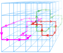
Figure 15: Illustration of the lattice worldline formalism. The gray dot indicates the base point ${\bm{x}}$.

Note that the number of hops $n$ must be even for closed paths on a cubic lattice, $n=2m$. The total number of paths of length $n$ on a $d$-dimensional lattice is $(2d)^{n}$. The mass introduces an exponential suppression of the weight of long paths in the sum over the length $n$ in eq. (212), since we can bound the summand by $(d/\tilde{d})^{n}=(1+\tfrac{m^{2}a^{2}}{2d})^{-n}$. The number of closed paths of length $n=2m$ is given by the following formula

$$\sum_{\gamma\in\Gamma_{2m}({\bm{x}},{\bm{x}})}1=\sum_{n_{1}+\cdots+n_{d}=m}\frac{(2m)!}{n_{1}!^{2}\cdots n_{d}!^{2}}\;,$$ (213)

and although it is considerably smaller than the total number of paths, it grows too quickly for an exhaustive enumeration of all the closed paths to reach the cutoff imposed by the mass. In refs. [112, 113, 114], it was proposed to depart from an exhaustive listing of the loops, and to use instead a statistical sampling that spans a much larger range of lengths. The ensemble of loops needs to be generated only once for a given set of lattice parameters, and can be reused for any background field on this lattice. Note however that, it may be advantageous to choose the ensemble of loops according to the physical length scale relevant for the problem under consideration (which in turn depends on the strength of the background field).

6.5 Worldline instanton approximation

Let us finally discuss a semi-classical approximation of the worldline expression of the 1-loop effective action [105, 106, 122, 123, 124, 125], which bears some resemblance with instantons in the fictitious time. For this reason, these semi-classical solutions are called worldline instantons. The starting point is the worldline representation of eq. (185) for the 1-loop effective action. By defining $\tau^{\prime}\equiv\tau u$ and $m^{2}\tau=s$, we can firstly rewrite it as

$${\cal V}_{{}_{E},\rm 1\ loop}=-\int_{0}^{\infty}\frac{ds}{s}\;e^{-s}\;\int\limits_{x^{i}(0)=x^{i}(1)}\big{[}{\cal D}x^{i}(u)\big{]}\;\exp\Big{(}-\Big{(}\frac{m^{2}}{4s}\int_{0}^{1}du\;\frac{\dot{x}^{2}}{4}+ie\int_{0}^{1}du\;\dot{x}^{i}A^{i}(x)\Big{)}\Big{)}\;,$$ (214)

where the path integration is now over closed loops of period 1. Since the rescaled fictitious time does not appear any longer as the integration bound inside the exponential, the integral over $s$ can be performed in closed form, yielding a Bessel function:

$${\cal V}_{{}_{E},\rm 1\ loop}=-2\int\limits_{x^{i}(0)=x^{i}(1)}\big{[}{\cal D}x^{i}(u)\big{]}\;K_{0}\left(\sqrt{m\int_{0}^{1}du\;\dot{x}^{2}}\right)\;\exp\Big{(}-ie\int_{0}^{1}du\;\dot{x}^{i}A^{i}(x)\Big{)}\;.$$ (215)

In the regime where

$$m^{2}\int_{0}^{1}du\,\dot{x}^{2}\gg 1\;,$$ (216)

whose physical significance will be clarified later, it is possible to replace the Bessel function by the first term of its asymptotic expansion,

$$K_{0}(z)\mathrel{\mathop{\kern 0.0pt\approx}\limits_{z\gg 1}}\sqrt{\frac{\pi}{2}}\;\frac{e^{-z}}{\sqrt{z}}\;.$$ (217)

This approximation leads to

$${\cal V}_{{}_{E},\rm 1\ loop} \approx -\sqrt{\frac{2\pi}{m}}\int\limits_{x^{i}(0)=x^{i}(1)}\big{[}{\cal D}x^{i}(u)\big{]}\;\left({\int_{0}^{1}du\;\dot{x}^{2}}\right)^{-1/4}$$ (218)

$$\qquad\qquad\times\,\exp\Big{(}-\Big{(}m\sqrt{\int_{0}^{1}du\;\dot{x}^{2}}+ie\int_{0}^{1}du\;\dot{x}^{i}A^{i}(x)\Big{)}\Big{)}\;.$$

The remaining path integral can be approximated by a stationary phase approximation, if we define the action

$${\cal S}\equiv m\sqrt{\int_{0}^{1}du\;\dot{x}^{2}}+ie\int_{0}^{1}du\;\dot{x}^{i}A^{i}(x)\;.$$ (219)

The stationarity condition is fulfilled for a closed path $x^{i}(u)$ that satisfies

$$m\frac{\ddot{x}^{i}}{\sqrt{\int_{0}^{1}du\;\dot{x}^{2}}}=ieF^{ij}\dot{x}^{j}\;,$$ (220)

where $F^{ij}$ is the strength of the background field. Since $F^{ij}$ must be evaluated at the point $x(u)$, this equation is a very non-trivial set of ordinary differential equations. By contracting eq. (220) with $\dot{x}^{i}$, the right hand side vanishes thanks to the antisymmetry of $F^{ij}$ and we therefore learn that

$$\dot{x}^{i}\dot{x}^{i}=\mbox{const}\equiv v^{2}\;.$$ (221)

The condition of eq. (216) is thus equivalent to $mv\gg 1$. For each solution of the stationarity condition (220), the corresponding extremal value of the action gives a contribution to the imaginary part of the effective action

$${\rm Im}\,{\cal V}_{{}_{E},\rm 1\ loop}\sim e^{-{\cal S}_{\rm extremum}}\;.$$ (222)

Note that a more complicated calculation, involving the calculation of the determinant of the Gaussian fluctuations around these stationary solutions, is required in order to determine the prefactor in front of the exponential.

In order to illustrate this method, let us consider the case of a spatially dependent Sauter field

$$E(x^{3})\equiv\frac{E}{\cosh^{2}(kx^{3})}\;,$$ (223)

that can be derived from the following gauge potential

$$A^{4}=-i\,\frac{E}{k}\,\tanh(kx^{3})\;.$$ (224)

The equations of motion for the stationary solutions are

$$\dot{x}^{3}=v\sqrt{1-\gamma^{-2}\tanh^{2}(kx^{3})}\;,\qquad\dot{x}^{4}=-\gamma^{-1}v\,\tanh(kx^{3})\;,$$ (225)

where $\gamma\equiv mk/(eE)$. There is a countable infinity of closed paths that satisfy these equations can be parameterized by

$$x^{3}(u) = \frac{m}{eE}\,\frac{1}{\gamma}\,{\rm arcsinh}\,\left(\frac{\gamma}{\sqrt{1-\gamma^{2}}}\,\sin(2\pi n\,u)\right)$$

$$x^{4}(u) = \frac{m}{eE}\,\frac{1}{\gamma\sqrt{1-\gamma^{2}}}\,{\rm arcsin}\,(\gamma\,\cos(2\pi n\,u))\;,$$ (226)

where $n$ is a strictly positive integer and $u\in[0,1]$. The index $n$ corresponds to how many times the closed path is traveled by the instanton solution.

In the limit of an extended field, $\gamma\to 0$, these closed paths become circular (one could have checked directly that the closed paths that extremalize the action in the case of a constant and homogeneous electrical field are indeed circles). In contrast, when $\gamma$ increases, these orbits become more and more elongated in the $x^{4}$ direction (see the figure 16) and they become infinitely large when $\gamma$ reaches unity (because of the prefactor $1/\sqrt{1-\gamma^{2}}$ in the second of eqs. (226)).

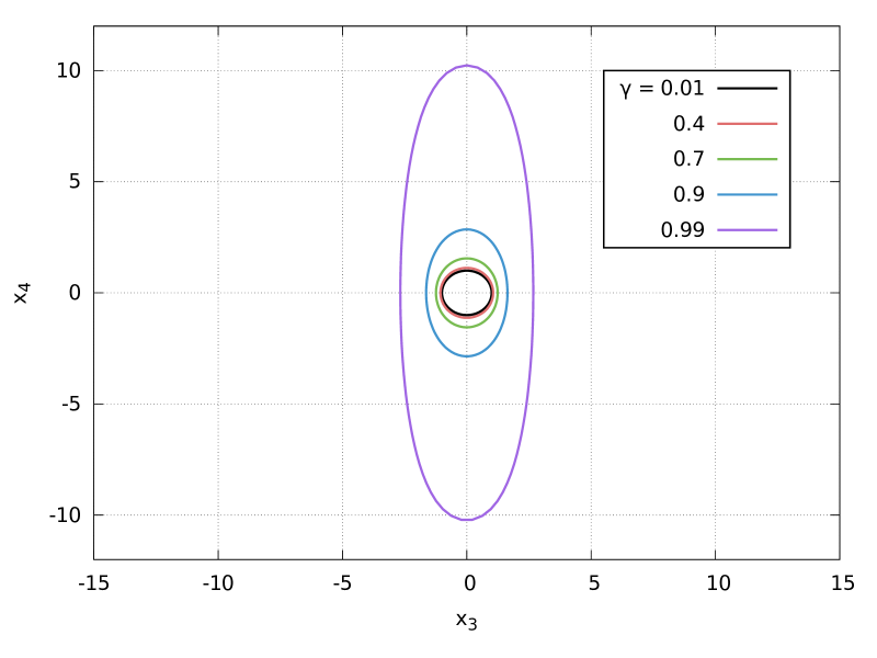
Figure 16: Closed paths in the $(x_{3},x_{4})$ plane of the instanton solutions in the case of an $x_{3}$-dependent Sauter electrical field, for various values of the parameter $\gamma\equiv mk/(eE)$. $\gamma=0$ corresponds to a circle of radius 1, and the closed paths become more and more elongated in the $x_{4}$ direction as $\gamma$ increases.

In this limit, the value of the stationary action becomes infinite, and the rate of particle production goes to zero. This result was of course known from the exact solution to particle production problem in the Sauter field. Physically, it reflects the fact that a field must exist over a spatial domain as large as one Compton wavelength in order to be able to produce particles. This simple academic example is an illustration of a more general phenomenon, namely that spatial inhomogeneities tend to decrease particle production (this reduction can become total when the field becomes incoherent over scales comparable to the Compton wavelength).

7 Dynamically assisted Schwinger mechanism

7.1 Comparison of perturbative and non-perturbative particle production

As indicated by the form of the factor $\exp(-{\pi m^{2}}/{(eE)})$, the Schwinger mechanism in a constant field is completely nonperturbative, even in a weak field regime $eE\ll m^{2}$. This is because the field is time-independent, and therefore no process initiated by a finite number of photons can produce the energy of a pair. If the electrical field has a time dependence, a perturbative component can also contribute particle production [117]. The transition between the perturbative regime and the non-perturbative regime can be characterized by the following dimensionless parameter,

$$\gamma\equiv\frac{m}{eE\tau}\;,$$ (227)

where $\tau$ is a characteristic time-scale of the time-dependence of the electrical field. This parameter has first been introduced by Keldysh in the context of the ionization of atoms [126], and is therefore called Keldysh parameter. In this subsection, by using an analytically solvable time-dependent field, we explicitly show how the transition between the perturbative and the nonperturbative regimes happens [51, 127].

Firstly, let us consider the distribution function obtained in a perturbative expansion up to the first order in a general background field. Since the distribution function is expressed by the mode function $\psi_{{\bm{p}},s}^{-}(x)$, we need to find the perturbative solution of the equation for the mode function,

$$\left[i\gamma^{\mu}D_{\mu}-m\right]\psi_{{\bm{p}},s}^{-}(x)=0\;.$$ (228)

It can be easily obtained from the Green’s formula

$$\psi(x)=\int_{y^{0}=t_{0}}d^{3}{\bm{y}}\;D_{R}^{0}(x,y)\;\gamma^{0}\,\psi(y)-ie\int_{y^{0}>t_{0}}d^{4}y\;D_{R}^{0}(x,y)\;\raise 0.6458pt\hbox{$/$}\kern-7.29996pt\hbox{$A$}(y)\,\psi(y)\;,$$ (229)

where $D_{R}^{0}(x,y)$ is the free retarded fermion propagator:

$$D_{R}^{0}(x,y)=\int\frac{d^{4}q}{(2\pi)^{4}}\frac{i(\raise 0.43057pt\hbox{$/$}\kern-5.29999pt\hbox{$q$}+m)}{q^{2}-m^{2}+iq^{0}\epsilon}e^{-iq\cdot(x-y)}\;.$$ (230)

By taking the limit of $t_{0}\to-\infty$ and using the boundary condition (85), one can see that the first term in the right hand side of eq. (229) is simply the free spinor, propagated from $t_{0}$ to $t$. Therefore, the Green’s formula also reads

$$\psi_{{\bm{p}},s}^{-}(x)=\psi_{{\bm{p}},s}^{\text{free}-}(x)-ie\int d^{4}y\;D_{R}^{0}(x,y)\;\raise 0.6458pt\hbox{$/$}\kern-7.29996pt\hbox{$A$}(y)\,\psi_{{\bm{p}},s}^{-}(y)\;.$$ (231)

This equation has an iterative solution

$$\psi_{{\bm{p}},s}^{-}(x)=\sum_{n=0}^{\infty}\psi_{{\bm{p}},s}^{(n)-}(x)\;,$$ (232)

where

$$\psi_{{\bm{p}},s}^{(n)-}(x)=(-ie)^{n}\int d^{4}y_{1}\cdots\int d^{4}y_{n}\;D_{R}^{0}(x,y_{1})\;\raise 0.6458pt\hbox{$/$}\kern-7.29996pt\hbox{$A$}(y_{1})\cdots D_{R}^{0}(y_{n-1},y_{n})\;\raise 0.6458pt\hbox{$/$}\kern-7.29996pt\hbox{$A$}(y_{n})\,\psi_{{\bm{p}},s}^{\text{free}-}(y_{n})\;.$$ (233)

This formula describes the correction to the spinor due to $n$ scatterings off the external field.

From the iterative solution (232), we can easily obtain the spectrum (108) at the first non-zero order in $e$. At this order, the gauge rotation factor $U(x)$ has no effect (it alters the spectrum only in higher orders). Therefore the spin-averaged spectrum at the lowest-order reads

$$\frac{dN^{(1)}}{d^{3}{\bm{p}}} = \frac{e^{2}}{(2\pi)^{3}2E_{\bm{p}}}\frac{1}{2}\sum_{s,s^{\prime}}\int\frac{d^{3}{\bm{p}}^{\prime}}{(2\pi)^{3}2E_{{\bm{p}}^{\prime}}}$$ (234)

$$\times\,\lim_{x^{0}\to+\infty}\Big{|}\bar{u}({\bm{p}},s)\int\frac{dq^{0}}{2\pi}\;\frac{e^{-iq^{0}x^{0}}}{q^{0}-E_{\bm{p}}+i\epsilon}\,\tilde{\raise 0.6458pt\hbox{$/$}\kern-7.29996pt\hbox{$A$}}(q^{0}+E_{{\bm{p}}^{\prime}},{\bm{p}}+{\bm{p}}^{\prime})v({\bm{p}}^{\prime},s^{\prime})\Big{|}^{2}\;,$$

where we have introduced

$$\tilde{A}^{\mu}(p)\equiv\int d^{4}x\;A^{\mu}(x)\;e^{ip\cdot x}\;.$$ (235)

This equation corresponds to computing the following 1-loop diagram:

If the Fourier-transformed gauge field $\tilde{A}(q^{0}+E_{{\bm{p}}^{\prime}},{\bm{p}}+{\bm{p}}^{\prime})$ contains no pole in the $q^{0}$-plane and is bounded when ${\rm Im}\,(q^{0})\to-\infty$, the $q^{0}$-integration can be performed by the theorem of residues by picking the pole of the prefactor $(q_{0}-E_{p}+i\epsilon)^{-1}$ (note that the exponential factor forces us to close the contour in lower half of the $q_{0}$ plane). After summing over the initial and final spin states, we have

$$\begin{split}\frac{dN^{(1)}}{d^{3}{\bm{p}}}&=\frac{2e^{2}}{(2\pi)^{3}2E_{\bm{p}}}\int\frac{d^{3}{\bm{p}}^{\prime}}{(2\pi)^{3}2E_{{\bm{p}}^{\prime}}}\;\left[p^{\mu}p^{\prime\,\nu}+p^{\nu}p^{\prime\,\mu}-(p\!\cdot\!p^{\prime}+m^{2})g^{\mu\nu}\right]\\ &\hskip 10.0pt\times\tilde{A}_{\mu}(E_{\bm{p}}+E_{{\bm{p}}^{\prime}},{\bm{p}}+{\bm{p}}^{\prime})\tilde{A}_{\nu}^{*}(E_{\bm{p}}+E_{{\bm{p}}^{\prime}},{\bm{p}}+{\bm{p}}^{\prime})\;,\end{split}$$ (236)

which is gauge invariant.

As an example, let us consider a sinusoidal time-dependent electrical field, $E_{z}(t)=E\,\cos(\omega t)$, for which the occupation number of the produced electrons is

$$\frac{(2\pi)^{3}}{V}\frac{dN^{(1)}}{d^{3}{\bm{p}}}=\frac{e^{2}E^{2}}{16E_{\bm{p}}^{2}}\;\left[1-\left(\frac{p_{z}}{E_{\bm{p}}}\right)^{2}\right]\;2\pi\delta(\omega-2E_{\bm{p}})\,T\;,$$ (237)

where $T\equiv 2\pi\delta(0)$ stands for the time duration of the electrical field. The proportionality of the result to this time $T$ is nothing but a manifestation of Fermi’s golden rule. This lowest-order spectrum corresponds to the process $\gamma\to e^{+}e^{-}$, where a single photon decays into an electron-positron pair. From the delta function, we see that this production mechanism is possible only if the frequency $\omega$ is above the threshold $2m$, as expected from energy momentum conservation.

To compare the lowest-order perturbative result with the non-perturbative all-order result, we use the Sauter-type pulsed field of eq. (123), which can be obtained from the gauge potential

$$A^{3}(t)=E\,\tau\tanh\left(\frac{t}{\tau}\right)\;.$$ (238)

The photons that make up this electrical field typically carry an energy $\omega\sim\tau^{-1}$. In this gauge field background, the lowest-order perturbative spectrum reads

$$\frac{(2\pi)^{3}}{V}\frac{dN^{(1)}}{d^{3}{\bm{p}}}=e^{2}E^{2}\;\left[1-\left(\frac{p_{z}}{E_{\bm{p}}}\right)^{2}\right]\;\frac{\pi^{2}\tau^{4}}{\sinh^{2}(\pi E_{\bm{p}}\tau)}\;.$$ (239)

Because the gauge field (238) has a continuous spectrum in Fourier space, the perturbative production does not display any threshold behavior. Unlike with the sinusoidal electrical field, the particle production happens for any value of the pulse characteristic timescale $\tau$. However, the particle production is most efficient if the photon energy is near the energy of the produced pair, $2E_{\bm{p}}$. Indeed, as a function of $\tau$, the spectrum has a peak around $E_{\bm{p}}\tau\simeq 0.61$.

The exact result for the spectrum in the same background, that includes the interaction with the background gauge field to all orders, is given by eq. (124). When changing the pulse duration $\tau$, this spectrum has a clear transition between the perturbative regime and the non-perturbative regime [127]. Since we have three dimensionful quantities, $m$, $eE$, and $\tau$, the system is governed by two dimensionless parameters,

$$\gamma\equiv\frac{m}{eE\tau}\;,\qquad\lambda\equiv eE\tau^{2}\;.$$ (240)

Taking the limit $\tau\to+\infty$ (limit of constant electrical field) while keeping $m$ and $eE$ constant corresponds to $\gamma\ll 1$ and $\lambda\gg 1$. One can confirm that the exact spectrum (124) goes to the spectrum due to a constant electrical field in this limit:

$$\frac{(2\pi)^{3}}{V}\frac{dN}{d^{3}{\bm{p}}}\qquad\xrightarrow[\gamma\ll 1,\ \lambda\gg 1]{}\qquad\exp\left(-\frac{\pi m_{\perp}^{2}}{eE}\right)\;.$$ (241)

At the other extreme, let us consider the short pulse limit, $\tau\to+\infty$, while keeping $m$ and $eE$ fixed. In terms of the dimensionless parameters $\gamma$ and $\lambda$, this limit corresponds to $\gamma\gg 1$ and $\lambda\ll 1$. Note that taking the limit $eE\to 0$ while keeping $m$ and $\tau$ fixed would also provide the same behavior of $\gamma$ and $\lambda$. Therefore, we expect that the lowest-order perturbative result (239) is recovered by this limit. Indeed, one can confirm that

$$\frac{(2\pi)^{3}}{V}\frac{dN}{d^{3}{\bm{p}}}\qquad\xrightarrow[\gamma\gg 1,\ \lambda\ll 1]{}\qquad e^{2}E^{2}\left[1-\left(\frac{p_{z}}{E_{\bm{p}}}\right)^{2}\right]\frac{\pi^{2}\tau^{4}}{\sinh^{2}(\pi E_{\bm{p}}\tau)}\;.$$ (242)

In order to illustrate this behavior, we plot the exact result (124) and the lowest-order result (239) for several values of the Keldysh parameter in the figure 17. The $p_{z}$-distributions at $p_{\perp}=0$ are shown in this plot. For large enough Keldysh parameter ($\gamma\gtrsim 20$), the two results show a good agreement. Conversely, as $\gamma$ gets smaller, the discrepancy becomes larger.

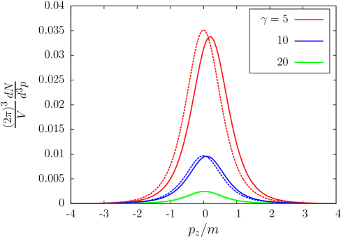
Figure 17: $p_{z}$-dependence of the spectrum at $p_{\perp}=0$. The all-order exact result (124) (solid lines) and the lowest-order perturbative result (239) (dashed lines) are compared for several values of the Keldysh parameter $\gamma$. The ratio $eE/m^{2}=1$ is fixed. For $\gamma=20$, the two lines are almost undistinguishable.

The transition between the perturbative regime and the non-perturbative regime is further illustrated in the figure 18. The maximum values of the momentum spectra (located at ${\bm{p}}=0$ for the perturbative spectrum, and at ${\bm{p}}=(0,0,eE\tau)$ for the all-order one) are compared as a function of $m\tau$, for several values of $eE/m^{2}$. The constant field Schwinger result $\exp(-{\pi m^{2}}/{(eE)})$ is also indicated by thin black lines for reference. The top figure shows the subcritical case $eE/m^{2}<1$, and the bottom figure shows the supercritical case $eE/m^{2}>1$. For small $\tau$ (large $\gamma$), the all-order result and the lowest-order one agree well. For large $\tau$ (small $\gamma$), the all-order result converges to the constant field Schwinger result, while the perturbative computation breaks down.

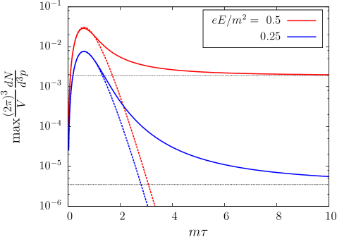
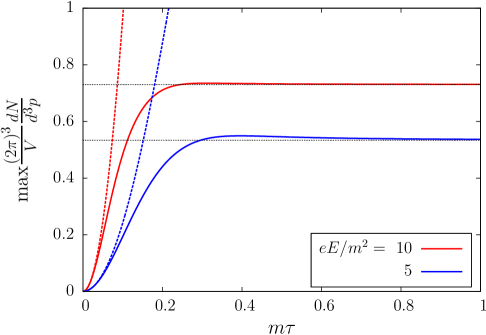
Figure 18: Plots of the maximum value of the momentum spectrum as a function of $m\tau$ for several values of $eE/m^{2}$. Top: subcritical field strength $eE/m^{2}<1$. Bottom: supercritical field strength $eE/m^{2}>1$. The all-order exact result (124) (solid lines) and the lowest-order perturbative result (239) (dashed lines) are compared. The constant field Schwinger result $\exp(-{\pi m^{2}}/(eE))$ is plotted as thin black lines.

What is remarkable in the left plot (subcritical case) is that the spectrum can be several orders of magnitude larger than the constant field Schwinger result in the regime $m\tau\sim 1$. This means that, in subcritical electrical fields, $eE/m^{2}<1$, a time-dependence of the electrical field dramatically amplifies the particle production, especially if the typical energy carried by the time-dependent electrical field is near the perturbative threshold $2m$.

7.2 Lattice numerical results

In the previous subsection, we have observed that the particle production in a time-dependent electrical field can be described by the lowest order perturbative calculation if the time-dependence is fast enough, such that $\gamma\gg 1$ and $\lambda\ll 1$. An important observation was that the particle production by the perturbative process $\gamma\to e^{+}e^{-}$ is much stronger than the non-perturbative Schwinger result if the field is subcritical $eE<m^{2}$ and the typical frequency of the time-dependent electrical field is near the threshold energy $2m$.

However, if the particle production is a purely perturbative process, it is not much interesting since perturbative processes are well understood theoretically and have been verified experimentally in many circumstances. Our main interest in this review is the particle production in the non-perturbative regime. As we shall see, a similar enhancement mechanism is realized also in the non-perturbative regime if the electrical field is a superposition of a slowly varying and strong (but still subcritical) field and a fast and weak field [128]. This phenomenon, called dynamically assisted Schwinger mechanism, has been the subject of many recent studies [129, 130, 131, 132, 133, 134, 135, 136], since it opens up the possibility that the non-perturbative electron-positron pair production may be observed more easily than expected in experiments [137, 138].

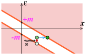
Figure 19: Schematic illustration of the dynamically assisted Schwinger mechanism.

To be specific, we consider a superposition of two Sauter time-dependent electrical fields

$$E_{z}(t)=\frac{E_{1}}{\cosh^{2}\big{(}\frac{t}{\tau_{1}}\big{)}}+\frac{E_{2}}{\cosh^{2}\big{(}\frac{t}{\tau_{2}}\big{)}}\;,$$ (243)

where $E_{1}\gg E_{2}$ and $\tau_{1}\gg\tau_{2}$ so that the first term represents a strong and slow field, while the second is a fast and weak field. In terms of the Keldysh parameter, these parameters are chosen so that $\gamma_{1}=\frac{m}{eE_{1}\tau_{1}}\ll 1$ and $\gamma_{2}=\frac{m}{eE_{2}\tau_{2}}\gg 1$. Therefore, the first pulse causes only non-perturbative particle production, while the second field can produce particles perturbatively. By superposing these two fields that have very different scales, an interplay between the non-perturbative and the perturbative physics occurs, leading to an important enhancement of the particle production.

Before presenting numerical evidence of this effect, let us qualitatively explain the mechanism at play. This is illustrated in the figure 19 (to be compared with the figure 1). In the standard Schwinger effect, a hole excitation must tunnel through the gap that separates the Dirac sea from the band of positive energy states, and there is therefore an exponential suppression in the length of this gap. As cartooned in the figure 19, a photon from the short weak field $E_{2}$ can slightly raise the energy of a hole excitation. But this effect alone is too weak to reach the positive energy band and produce an on-shell electron-positron pair. However, once it has been brought to this slightly higher energy, the hole excitation also has a shorter length to tunnel through in order to reach the positive energy band by quantum tunneling. Since the tunneling probability is exponentially sensitive to this length, even a moderate change in the length can produce an important increase in the yield. This is the essence of the dynamically assisted Schwinger mechanism.

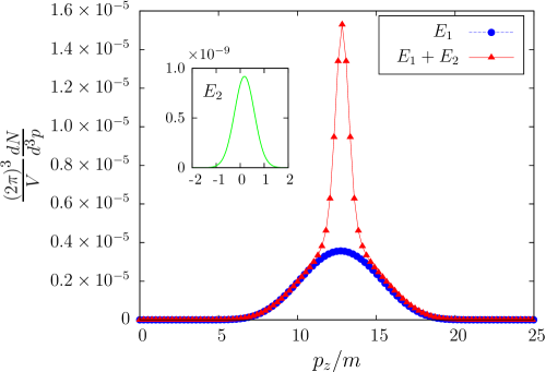
Figure 20: The momentum spectrum of electrons produced by the field (243) with the parameters $eE_{1}=0.25\,m_{e}^{2}$, $\tau_{1}=10^{-4}\ \text{eV}^{-1}$ and $eE_{2}=0.025\,m_{e}^{2}$, $\tau_{2}=7\times 10^{-6}\ \text{eV}^{-1}$. $p_{z}$-dependence at $p_{\perp}=0$ is shown. The curve labeled $E_{1}+E_{2}$ shows the particle spectrum resulting from the sum of the two fields, while the curves labeled $E_{1}$ and $E_{2}$ show the particle spectrum that results from the two fields considered separately.

Following ref. [132], we show the momentum spectra of particles produced in the electrical field (243). While the quantum kinetic approach was used in ref. [132], we present the same results computed by real-time lattice calculations in the mode function method. In the figure 20, the momentum spectrum with the parameters $eE_{1}=0.25\,m_{e}^{2}$, $\tau_{1}=10^{-4}\ \text{eV}^{-1}=510/m_{e}$ and $eE_{2}=0.025\,m_{e}^{2}$, $\tau_{2}=7\times 10^{-6}\ \text{eV}^{-1}=3.57/m_{e}$ is plotted. The Keldysh parameters for each pulse are $\gamma_{1}\simeq 0.078$, and $\gamma_{2}\simeq 11.2$, respectively. Therefore, the first pulse is in the non-perturbative regime, while the second is in the perturbative regime. For comparison, the spectrum produced by the strong and slow pulse (curve labeled $E_{1}$) alone and that by the single weak and fast pulse (curve labeled $E_{2}$) alone are also shown. Although the single pulse $E_{2}$ is extremely weak and the spectrum it produces by itself is several orders of magnitude smaller than the spectrum produced by the pulse $E_{1}$, superposing this weak and fast fields causes a dramatic enhancement of the production yield, by a factor around $4$.

In the lowest-order perturbative production studied in the previous subsection, the particle production is the most intense when the typical energy carried by photons constituting the electrical field is near to the threshold value $2m$. In the case of the single Sauter-type pulse, the particle yield by the lowest-order production takes maximum value when $m\tau\simeq 0.61$. Also in the case of the dynamically assisted Schwinger mechanism in the double pulse (243), the maximum enhancement occurs when the typical energy carried by the weak pulse is near to $2m$. In Fig. 21, the $p_{z}$-spectra are plotted for several values of $m_{e}\tau_{2}$. Other parameters are fixed to $eE_{1}=0.25\,m_{e}^{2}$, $m_{e}\tau_{1}=510$, and $eE_{2}=0.025\,m_{e}^{2}$. Within this parameter set, the enhancement is the most prominent at $m_{e}\tau_{2}\simeq 0.61$. Of course, the degree of the enhancement largely depends not only on $\tau_{2}$ but also on other parameters and the profile of the electrical field as well. Optimization of the field profile to gain the maximum particle yield has been investigated in refs. [139, 140, 141].

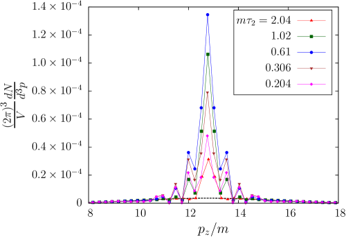
Figure 21: The momentum spectrum of electrons produced by the field (243) for several values of $m_{e}\tau_{2}$. The other parameters are fixed to $eE_{1}=0.25\,m_{e}^{2}$, $m_{e}\tau_{1}=510$ and $eE_{2}=0.025\,m_{e}^{2}$. The result with the single pulse $E_{1}$ is plotted as a black dashed line for comparison. The lattice parameters are the same as those in the figure 20.

8 Summary and conclusions

In this review, we have covered some of the recent works related to the study of the Schwinger mechanism. Our main motivation in this review has been to present methods that have been designed in order to cope with more general backgrounds than those for which exact analytical solutions exist, allowing (numerical) studies of pair production in backgrounds with arbitrary space-time dependences (for smooth enough dependences, one may instead use a derivative expansion of the effective action [143, 144]).

Two main classes of methods have been discussed in this review. The first one, that follows more conventional techniques of quantum field theory, is based on the possibility of expressing any one-loop amplitude in a background field in terms of mode functions. Loosely speaking, such one-loop amplitudes can be generated by small Gaussian fluctuations around a given background, and are therefore fully determined by the knowledge of a basis of small field perturbations about this background. This approach has a number of variants, that differ in the formulation but share common origins and are rigorously equivalent. The method of Bogoliubov transformations is directly connected to the mode functions by the fact that the Bogoliubov coefficients are obtained from the decomposition of the mode functions in Fourier modes. For spatially homogeneous electrical fields, it is possible to express the time evolution directly at the level of the Bogoliubov coefficients themselves, via quantum kinetic equations. These can be formulated either as two local in time equations for a pair of coupled distributions, one of which is the usual occupation number and the other is an anomalous distribution, or as a single equation, non-local in time, for the occupation number. When the background field is inhomogeneous, quantum kinetic equations can be generalized into an equation for the Wigner distribution of the system (i.e. the Wigner transform of the density operator).

The second family of methods that we have discussed in this review revolves around the worldline formalism, a formulation in which one-loop amplitudes in a background field are expressed as a path integration over all the closed paths in Euclidean space-time, parameterized by a extra fictitious time. Although it was originally derived from ideas in string theory, this representation has also some connections with Schwinger’s proper time formulation for propagators. For a constant and homogeneous background, this approach leads easily to the well known analytical one-loop answer. In other cases, such as the Sauter background electrical field, one can obtain approximations valid in the weak field regime by finding extrema of a 5-dimensional action, called worldline instantons due to their resemblance with ordinary instanton solutions. For even more general backgrounds, numerical methods have been developed, in which one samples statistically the ensemble of worldlines. Although completely equivalent to more conventional methods, the worldline formalism emphasizes the space-time development of the production process, and brings some useful intuition over the relevant phenomena (e.g. the fact that in weak fields large worldlines play a very important role).

Besides these developments in the technical tools available for theoretical studies of the Schwinger mechanism, a number of works have focused on finding the type of external fields that may maximize the yield of produced particles, following the simple observation that the superposition of two fields results in a particle spectrum which is not simply the sum of the spectra that these two fields would produce individually (because the Schwinger mechanism is highly non-linear in the field). A simple yet spectacular such effect is the dynamically assisted Schwinger mechanism, obtained by superimposing a slow but intense field with a fast and much weaker field, both of which are much lower than the critical field. Intuitively, the short pulse raises the energy of a hole excitation, thereby shortening the tunneling length it has to overcome in order to be produced on-shell and considerably enhancing the yield. These phenomena could be used in order to greatly facilitate the experimental production of pairs by the Schwinger mechanism.

Let us finish this section by listing several topics related to the Schwinger mechanism that were not discussed in any detail in this review. Firstly, all the discussion of pair production by external fields in electrodynamics can be carried through to strong interactions in quantum chromodynamics. The most direct extension obviously concerns quark production in a chromo-electrical field [145, 146, 92, 147, 148], but the Schwinger mechanism can also be relevant for gluon production [149, 54, 150, 151, 152]. In heavy-ion collisions at high energies, the system is approximately boost-invariant in the longitudinal beam direction. The Schwinger mechanism in such a boost invariant expanding geometry has been studied in refs. [87, 153]. In this review, we have only considered the case where the system is initially in the vacuum state. This can be generalized to situations where the system is initially non-empty, such as a thermal system [154, 155, 56, 156, 157, 158], where quantum statistical effects will alter the production rate of particles by the external field. In QCD, it has also been argued that the Schwinger mechanism may lead to the dynamical generation of a gluon mass, that could explain some features of the Landau gauge propagators and verticein the soft sector [159].

Besides the production of elementary particles by external fields in vacuum, the Schwinger mechanism can also lead to the production of quasi-particle excitations in more exotic materials such as graphene [160, 161, 162, 163, 164], where it may be easier to achieve experimentally. The possibility of using ultracold atoms in an optical lattice as a simulator for the Schwinger mechanism was considered in ref. [165].

Among the theoretical tools used to study the Schwinger mechanism, let us mention a proposal to use stochastic quantization in ref. [166], and some of the many works where holographic (e.g. based on the AdS/CFT correspondence) setups were considered in order to investigate particle production by external fields in the strong coupling regime [167, 168, 169, 170, 171, 172, 173, 174, 175, 176]. Let us also finally mention another recent review on the Schwinger mechanism more focused on the backreaction and applications in astrophysics [177], as well as some works on the closely related question of pair creation in a curved space-time [178, 179, 180, 181, 182, 183].

References

- [1] J. S. Schwinger, “On gauge invariance and vacuum polarization,” Phys. Rev. 82 (1951) 664–679.
- [2] F. Sauter, “Uber das Verhalten eines Elektrons im homogenen elektrischen Feld nach der relativistischen Theorie Diracs,” Z. Phys. 69 (1931) 742–764.
- [3] W. Heisenberg and H. Euler, “Consequences of Dirac’s theory of positrons,” Z. Phys. 98 (1936) 714–732, arXiv:physics/0605038 [physics].
- [4] C. Itzykson and J. B. Zuber, Quantum Field Theory. 1980. http://dx.doi.org/10.1063/1.2916419.
- [5] T. S. Biro, H. B. Nielsen, and J. Knoll, “Color Rope Model for Extreme Relativistic Heavy Ion Collisions,” Nucl. Phys. B245 (1984) 449–468.
- [6] K. Kajantie and T. Matsui, “Decay of Strong Color Electric Field and Thermalization in Ultrarelativistic Nucleus-Nucleus Collisions,” Phys. Lett. B164 (1985) 373.
- [7] G. Gatoff, A. K. Kerman, and T. Matsui, “The Flux Tube Model for Ultrarelativistic Heavy Ion Collisions: Electrohydrodynamics of a Quark Gluon Plasma,” Phys. Rev. D36 (1987) 114.
- [8] D. Kharzeev, E. Levin, and K. Tuchin, “Multi-particle production and thermalization in high-energy QCD,” Phys. Rev. C75 (2007) 044903, arXiv:hep-ph/0602063 [hep-ph].
- [9] B. Andersson, G. Gustafson, G. Ingelman, and T. Sjostrand, “Parton Fragmentation and String Dynamics,” Phys. Rept. 97 (1983) 31–145.
- [10] L. D. McLerran and R. Venugopalan, “Computing quark and gluon distribution functions for very large nuclei,” Phys. Rev. D49 (1994) 2233–2241, arXiv:hep-ph/9309289 [hep-ph].
- [11] L. D. McLerran and R. Venugopalan, “Gluon distribution functions for very large nuclei at small transverse momentum,” Phys. Rev. D49 (1994) 3352–3355, arXiv:hep-ph/9311205 [hep-ph].
- [12] F. Gelis and R. Venugopalan, “Particle production in field theories coupled to strong external sources,” Nucl. Phys. A776 (2006) 135–171, arXiv:hep-ph/0601209 [hep-ph].
- [13] F. Gelis and R. Venugopalan, “Particle production in field theories coupled to strong external sources. II. Generating functions,” Nucl. Phys. A779 (2006) 177–196, arXiv:hep-ph/0605246 [hep-ph].
- [14] R. E. Cutkosky, “Singularities and discontinuities of Feynman amplitudes,” J. Math. Phys. 1 (1960) 429–433.
- [15] G. ’t Hooft and M. J. G. Veltman, “Diagrammar,” NATO Sci. Ser. B 4 (1974) 177–322.
- [16] J. S. Schwinger, “Brownian motion of a quantum oscillator,” J. Math. Phys. 2 (1961) 407–432.
- [17] L. V. Keldysh, “Diagram technique for nonequilibrium processes,” Zh. Eksp. Teor. Fiz. 47 (1964) 1515–1527. [Sov. Phys. JETP20,1018(1965)].
- [18] E. Iancu, A. Leonidov, and L. D. McLerran, “Nonlinear gluon evolution in the color glass condensate. 1.,” Nucl. Phys. A692 (2001) 583–645, arXiv:hep-ph/0011241 [hep-ph].
- [19] E. Ferreiro, E. Iancu, A. Leonidov, and L. McLerran, “Nonlinear gluon evolution in the color glass condensate. 2.,” Nucl. Phys. A703 (2002) 489–538, arXiv:hep-ph/0109115 [hep-ph].
- [20] E. Iancu, A. Leonidov, and L. McLerran, “The Color glass condensate: An Introduction,” in QCD perspectives on hot and dense matter. Proceedings, NATO Advanced Study Institute, Summer School, Cargese, France, August 6-18, 2001, pp. 73–145. 2002. arXiv:hep-ph/0202270 [hep-ph]. http://alice.cern.ch/format/showfull?sysnb=2297268.
- [21] E. Iancu and R. Venugopalan, “The Color glass condensate and high-energy scattering in QCD,” in In *Hwa, R.C. (ed.) et al.: Quark gluon plasma* 249-3363. 2003. arXiv:hep-ph/0303204 [hep-ph].
- [22] H. Weigert, “Evolution at small x(bj): The Color glass condensate,” Prog. Part. Nucl. Phys. 55 (2005) 461–565, arXiv:hep-ph/0501087 [hep-ph].
- [23] F. Gelis, T. Lappi, and R. Venugopalan, “High energy scattering in Quantum Chromodynamics,” Int. J. Mod. Phys. E16 (2007) 2595–2637, arXiv:0708.0047 [hep-ph].
- [24] F. Gelis, E. Iancu, J. Jalilian-Marian, and R. Venugopalan, “The Color Glass Condensate,” Ann. Rev. Nucl. Part. Sci. 60 (2010) 463–489, arXiv:1002.0333 [hep-ph].
- [25] F. Gelis, “Color Glass Condensate and Glasma,” Int. J. Mod. Phys. A28 (2013) 1330001, arXiv:1211.3327 [hep-ph].
- [26] A. Kovner, L. D. McLerran, and H. Weigert, “Gluon production from nonAbelian Weizsacker-Williams fields in nucleus-nucleus collisions,” Phys. Rev. D52 (1995) 6231–6237, arXiv:hep-ph/9502289 [hep-ph].
- [27] Y. V. Kovchegov and D. H. Rischke, “Classical gluon radiation in ultrarelativistic nucleus-nucleus collisions,” Phys. Rev. C56 (1997) 1084–1094, arXiv:hep-ph/9704201 [hep-ph].
- [28] A. Krasnitz and R. Venugopalan, “Nonperturbative computation of gluon minijet production in nuclear collisions at very high-energies,” Nucl. Phys. B557 (1999) 237, arXiv:hep-ph/9809433 [hep-ph].
- [29] A. Krasnitz and R. Venugopalan, “The Initial energy density of gluons produced in very high-energy nuclear collisions,” Phys. Rev. Lett. 84 (2000) 4309–4312, arXiv:hep-ph/9909203 [hep-ph].
- [30] A. Krasnitz, Y. Nara, and R. Venugopalan, “Coherent gluon production in very high-energy heavy ion collisions,” Phys. Rev. Lett. 87 (2001) 192302, arXiv:hep-ph/0108092 [hep-ph].
- [31] T. Lappi, “Production of gluons in the classical field model for heavy ion collisions,” Phys. Rev. C67 (2003) 054903, arXiv:hep-ph/0303076 [hep-ph].
- [32] T. Lappi and L. McLerran, “Some features of the glasma,” Nucl. Phys. A772 (2006) 200–212, arXiv:hep-ph/0602189 [hep-ph].
- [33] F. Gelis, T. Lappi, and L. McLerran, “Glittering Glasmas,” Nucl. Phys. A828 (2009) 149–160, arXiv:0905.3234 [hep-ph].
- [34] B. Schenke, P. Tribedy, and R. Venugopalan, “Fluctuating Glasma initial conditions and flow in heavy ion collisions,” Phys. Rev. Lett. 108 (2012) 252301, arXiv:1202.6646 [nucl-th].
- [35] F. Gelis, T. Lappi, and R. Venugopalan, “High energy factorization in nucleus-nucleus collisions. II. Multigluon correlations,” Phys. Rev. D78 (2008) 054020, arXiv:0807.1306 [hep-ph].
- [36] F. Gelis, T. Lappi, and R. Venugopalan, “High energy factorization in nucleus-nucleus collisions. 3. Long range rapidity correlations,” Phys. Rev. D79 (2009) 094017, arXiv:0810.4829 [hep-ph].
- [37] S. A. Voloshin, “Transverse radial expansion in nuclear collisions and two particle correlations,” Phys. Lett. B632 (2006) 490–494, arXiv:nucl-th/0312065 [nucl-th].
- [38] E. V. Shuryak, “On the origin of the ’Ridge’ phenomenon induced by jets in heavy ion collisions,” Phys. Rev. C76 (2007) 047901, arXiv:0706.3531 [nucl-th].
- [39] PHENIX Collaboration, A. Adare et al., “Dihadron azimuthal correlations in Au+Au collisions at s(NN)**(1/2) = 200-GeV,” Phys. Rev. C78 (2008) 014901, arXiv:0801.4545 [nucl-ex].
- [40] PHOBOS Collaboration, B. Alver et al., “System size dependence of cluster properties from two-particle angular correlations in Cu+Cu and Au+Au collisions at s(NN)**(1/2) = 200-GeV,” Phys. Rev. C81 (2010) 024904, arXiv:0812.1172 [nucl-ex].
- [41] STAR Collaboration, B. I. Abelev et al., “Long range rapidity correlations and jet production in high energy nuclear collisions,” Phys. Rev. C80 (2009) 064912, arXiv:0909.0191 [nucl-ex].
- [42] PHOBOS Collaboration, B. Alver et al., “High transverse momentum triggered correlations over a large pseudorapidity acceptance in Au+Au collisions at s(NN)**1/2 = 200 GeV,” Phys. Rev. Lett. 104 (2010) 062301, arXiv:0903.2811 [nucl-ex].
- [43] A. Dumitru, F. Gelis, L. McLerran, and R. Venugopalan, “Glasma flux tubes and the near side ridge phenomenon at RHIC,” Nucl. Phys. A810 (2008) 91–108, arXiv:0804.3858 [hep-ph].
- [44] B. Alver and G. Roland, “Collision geometry fluctuations and triangular flow in heavy-ion collisions,” Phys. Rev. C81 (2010) 054905, arXiv:1003.0194 [nucl-th]. [Erratum: Phys. Rev.C82,039903(2010)].
- [45] B. H. Alver, C. Gombeaud, M. Luzum, and J.-Y. Ollitrault, “Triangular flow in hydrodynamics and transport theory,” Phys. Rev. C82 (2010) 034913, arXiv:1007.5469 [nucl-th].
- [46] F. Gelis, T. Lappi, and R. Venugopalan, “High energy factorization in nucleus-nucleus collisions,” Phys. Rev. D78 (2008) 054019, arXiv:0804.2630 [hep-ph].
- [47] F. Gelis, K. Kajantie, and T. Lappi, “Quark-antiquark production from classical fields in heavy ion collisions: 1+1 dimensions,” Phys. Rev. C71 (2005) 024904, arXiv:hep-ph/0409058 [hep-ph].
- [48] F. Gelis, K. Kajantie, and T. Lappi, “Chemical thermalization in relativistic heavy ion collisions,” Phys. Rev. Lett. 96 (2006) 032304, arXiv:hep-ph/0508229 [hep-ph].
- [49] F. Gelis and N. Tanji, “Quark production in heavy ion collisions I. Formalism and boost invariant fermionic light-cone mode functions,” arXiv:1506.03327 [hep-ph].
- [50] K. Fukushima, F. Gelis, and T. Lappi, “Multiparticle correlations in the Schwinger mechanism,” Nucl. Phys. A831 (2009) 184–214, arXiv:0907.4793 [hep-ph].
- [51] N. B. Narozhnyi and A. I. Nikishov, “The Simplist processes in the pair creating electric field,” Yad. Fiz. 11 (1970) 1072. [Sov. J. Nucl. Phys.11,596(1970)].
- [52] D. M. Gitman, “Processes of Arbitrary Order in Quantum Electrodynamics with a Pair Creating External Field,” J. Phys. A10 (1977) 2007–2020.
- [53] M. Soffel, B. Muller, and W. Greiner, “Stability and decay of the Dirac vacuum in external gauge fields,” Phys. Rept. 85 (1982) 51–122.
- [54] J. Ambjorn and R. J. Hughes, “Canonical Quantization in Nonabelian Background Fields. 1.,” Annals Phys. 145 (1983) 340.
- [55] S. P. Gavrilov and D. M. Gitman, “Vacuum instability in external fields,” Phys. Rev. D53 (1996) 7162–7175, arXiv:hep-th/9603152 [hep-th].
- [56] S. P. Gavrilov, D. M. Gitman, and J. L. Tomazelli, “Density matrix of a quantum field in a particle-creating background,” Nucl. Phys. B795 (2008) 645–677, arXiv:hep-th/0612064 [hep-th].
- [57] N. Tanji, “Dynamical view of pair creation in uniform electric and magnetic fields,” Annals Phys. 324 (2009) 1691–1736, arXiv:0810.4429 [hep-ph].
- [58] F. Sauter, “Zum kleinschen paradoxon,” Z. Phys. 73 no. 7, (1932) 547–552.
- [59] V. Popov and M. Marinov, “ pair production in an alternating electric-field,” Sov. J. Nucl. Phys. 16 no. 4, (1973) 449–456.
- [60] S. A. Smolyansky, G. Ropke, S. M. Schmidt, D. Blaschke, V. D. Toneev, and A. V. Prozorkevich, “Dynamical derivation of a quantum kinetic equation for particle production in the Schwinger mechanism,” arXiv:hep-ph/9712377 [hep-ph].
- [61] S. M. Schmidt, D. Blaschke, G. Ropke, S. A. Smolyansky, A. V. Prozorkevich, and V. D. Toneev, “A Quantum kinetic equation for particle production in the Schwinger mechanism,” Int. J. Mod. Phys. E7 (1998) 709–722, arXiv:hep-ph/9809227 [hep-ph].
- [62] Y. Kluger, E. Mottola, and J. M. Eisenberg, “The Quantum Vlasov equation and its Markov limit,” Phys. Rev. D58 (1998) 125015, arXiv:hep-ph/9803372 [hep-ph].
- [63] R. Micha and I. I. Tkachev, “Turbulent thermalization,” Phys. Rev. D70 (2004) 043538, arXiv:hep-ph/0403101 [hep-ph].
- [64] I. Bialynicki-Birula, P. Gornicki, and J. Rafelski, “Phase space structure of the Dirac vacuum,” Phys. Rev. D44 (1991) 1825–1835.
- [65] P. Levai and V. Skokov, “Nonperturbative enhancement of heavy quark-pair production in a strong SU(2) color field,” Phys. Rev. D82 (2010) 074014, arXiv:0909.2323 [hep-ph].
- [66] F. Hebenstreit, R. Alkofer, and H. Gies, “Schwinger pair production in space and time-dependent electric fields: Relating the Wigner formalism to quantum kinetic theory,” Phys. Rev. D82 (2010) 105026, arXiv:1007.1099 [hep-ph].
- [67] F. Hebenstreit, A. Ilderton, M. Marklund, and J. Zamanian, “Strong field effects in laser pulses: the Wigner formalism,” Phys. Rev. D83 (2011) 065007, arXiv:1011.1923 [hep-ph].
- [68] F. Hebenstreit, R. Alkofer, and H. Gies, “Particle self-bunching in the Schwinger effect in spacetime-dependent electric fields,” Phys. Rev. Lett. 107 (2011) 180403, arXiv:1106.6175 [hep-ph].
- [69] D. Berényi, S. Varró, V. V. Skokov, and P. Lévai, “Pair production at the edge of the QED flux tube,” Phys. Lett. B749 (2015) 210–214, arXiv:1401.0039 [hep-ph].
- [70] G. Aarts and J. Smit, “Real time dynamics with fermions on a lattice,” Nucl. Phys. B555 (1999) 355–394, arXiv:hep-ph/9812413 [hep-ph].
- [71] G. Aarts and J. Smit, “Particle production and effective thermalization in inhomogeneous mean field theory,” Phys. Rev. D61 (2000) 025002, arXiv:hep-ph/9906538 [hep-ph].
- [72] F. Gelis and N. Tanji, “Formulation of the Schwinger mechanism in classical statistical field theory,” Phys. Rev. D87 no. 12, (2013) 125035, arXiv:1303.4633 [hep-ph].
- [73] S. Borsanyi and M. Hindmarsh, “Low-cost fermions in classical field simulations,” Phys.Rev. D79 (2009) 065010, arXiv:0809.4711 [hep-ph].
- [74] P. M. Saffin and A. Tranberg, “Real-time Fermions for Baryogenesis Simulations,” JHEP 1107 (2011) 066, arXiv:1105.5546 [hep-ph].
- [75] P. M. Saffin and A. Tranberg, “Dynamical simulations of electroweak baryogenesis with fermions,” JHEP 1202 (2012) 102, arXiv:1111.7136 [hep-ph].
- [76] J. Berges, D. Gelfand, and D. Sexty, “Amplified Fermion Production from Overpopulated Bose Fields,” Phys.Rev. D89 no. 2, (2014) 025001, arXiv:1308.2180 [hep-ph].
- [77] V. Kasper, F. Hebenstreit, and J. Berges, “Fermion production from real-time lattice gauge theory in the classical-statistical regime,” Phys.Rev. D90 no. 2, (2014) 025016, arXiv:1403.4849 [hep-ph].
- [78] S. P. Gavrilov and D. M. Gitman, “One-loop energy-momentum tensor in QED with electric-like background,” Phys. Rev. D78 (2008) 045017, arXiv:0709.1828 [hep-th].
- [79] S. P. Gavrilov and D. M. Gitman, “Consistency restrictions on maximal electric field strength in QFT,” Phys. Rev. Lett. 101 (2008) 130403, arXiv:0805.2391 [hep-th].
- [80] A. Casher, J. B. Kogut, and L. Susskind, “Vacuum polarization and the absence of free quarks,” Phys. Rev. D10 (1974) 732–745.
- [81] N. K. Glendenning and T. Matsui, “Creation of anti-Q Q pair in a chromoelectric flux tube,” Phys. Rev. D28 (1983) 2890–2891.
- [82] F. Hebenstreit, J. Berges, and D. Gelfand, “Real-time dynamics of string breaking,” Phys. Rev. Lett. 111 (2013) 201601, arXiv:1307.4619.
- [83] F. Cooper and E. Mottola, “Quantum Back Reaction in Scalar QED as an Initial Value Problem,” Phys. Rev. D40 (1989) 456.
- [84] Y. Kluger, J. M. Eisenberg, B. Svetitsky, F. Cooper, and E. Mottola, “Pair production in a strong electric field,” Phys. Rev. Lett. 67 (1991) 2427–2430.
- [85] Y. Kluger, J. M. Eisenberg, B. Svetitsky, F. Cooper, and E. Mottola, “Fermion pair production in a strong electric field,” Phys. Rev. D45 (1992) 4659–4671.
- [86] Y. Kluger, J. M. Eisenberg, and B. Svetitsky, “Pair production in a strong electric field: An Initial value problem in quantum field theory,” Int. J. Mod. Phys. E2 (1993) 333–380, arXiv:hep-ph/0311293 [hep-ph].
- [87] F. Cooper, J. M. Eisenberg, Y. Kluger, E. Mottola, and B. Svetitsky, “Particle production in the central rapidity region,” Phys. Rev. D48 (1993) 190–208, arXiv:hep-ph/9212206 [hep-ph].
- [88] J. F. Dawson, B. Mihaila, and F. Cooper, “Fermion particle production in semi-classical Boltzmann-Vlasov transport theory,” Phys. Rev. D80 (2009) 014011, arXiv:0906.2225 [hep-ph].
- [89] M. Asakawa and T. Matsui, “Dilepton production from a nonequilibrium quark - gluon plasma in ultrarelativistic nucleus-nucleus collisions,” Phys. Rev. D43 (1991) 2871–2891.
- [90] D. V. Vinnik, A. V. Prozorkevich, S. A. Smolyansky, V. D. Toneev, M. B. Hecht, C. D. Roberts, and S. M. Schmidt, “Plasma production and thermalization in a strong field,” Eur. Phys. J. C22 (2001) 341–349, arXiv:nucl-th/0103073 [nucl-th].
- [91] J. C. R. Bloch, V. A. Mizerny, A. V. Prozorkevich, C. D. Roberts, S. M. Schmidt, S. A. Smolyansky, and D. V. Vinnik, “Pair creation: Back reactions and damping,” Phys. Rev. D60 (1999) 116011, arXiv:nucl-th/9907027 [nucl-th].
- [92] N. Tanji, “Quark pair creation in color electric fields and effects of magnetic fields,” Annals Phys. 325 (2010) 2018–2040, arXiv:1002.3143 [hep-ph].
- [93] F. Hebenstreit, J. Berges, and D. Gelfand, “Simulating fermion production in 1+1 dimensional QED,” Phys. Rev. D87 no. 10, (2013) 105006, arXiv:1302.5537 [hep-ph].
- [94] S. Habib, Y. Kluger, E. Mottola, and J. P. Paz, “Dissipation and decoherence in mean field theory,” Phys. Rev. Lett. 76 (1996) 4660–4663, arXiv:hep-ph/9509413 [hep-ph].
- [95] R. R. Metsaev and A. A. Tseytlin, “On loop corrections to string theory effective actions,” Nucl. Phys. B298 (1988) 109.
- [96] Z. Bern and D. A. Kosower, “A New Approach to One Loop Calculations in Gauge Theories,” Phys. Rev. D38 (1988) 1888.
- [97] Z. Bern and D. A. Kosower, “Efficient calculation of one loop QCD amplitudes,” Phys. Rev. Lett. 66 (1991) 1669–1672.
- [98] M. J. Strassler, “Field theory without Feynman diagrams: One loop effective actions,” Nucl. Phys. B385 (1992) 145–184, arXiv:hep-ph/9205205 [hep-ph].
- [99] C. Schubert, “An Introduction to the worldline technique for quantum field theory calculations,” Acta Phys. Polon. B27 (1996) 3965–4001, arXiv:hep-th/9610108 [hep-th].
- [100] C. Schubert, “Perturbative quantum field theory in the string inspired formalism,” Phys. Rept. 355 (2001) 73–234, arXiv:hep-th/0101036 [hep-th].
- [101] M. Reuter, M. G. Schmidt, and C. Schubert, “Constant external fields in gauge theory and the spin 0, 1/2, 1 path integrals,” Annals Phys. 259 (1997) 313–365, arXiv:hep-th/9610191 [hep-th].
- [102] M. G. Schmidt and C. Schubert, “On the calculation of effective actions by string methods,” Phys. Lett. B318 (1993) 438–446, arXiv:hep-th/9309055 [hep-th].
- [103] M. G. Schmidt and C. Schubert, “Multiloop calculations in the string inspired formalism: The Single spinor loop in QED,” Phys. Rev. D53 (1996) 2150–2159, arXiv:hep-th/9410100 [hep-th].
- [104] H. Gies, J. Sanchez-Guillen, and R. A. Vazquez, “Quantum effective actions from nonperturbative worldline dynamics,” JHEP 08 (2005) 067, arXiv:hep-th/0505275 [hep-th].
- [105] G. V. Dunne and C. Schubert, “Worldline instantons and pair production in inhomogeneous fields,” Phys. Rev. D72 (2005) 105004, arXiv:hep-th/0507174 [hep-th].
- [106] G. V. Dunne, Q.-h. Wang, H. Gies, and C. Schubert, “Worldline instantons. II. The Fluctuation prefactor,” Phys. Rev. D73 (2006) 065028, arXiv:hep-th/0602176 [hep-th].
- [107] H. Gies, K. Langfeld, and L. Moyaerts, “Casimir effect on the worldline,” JHEP 06 (2003) 018, arXiv:hep-th/0303264 [hep-th].
- [108] H. Gies and K. Klingmuller, “Worldline algorithms for Casimir configurations,” Phys. Rev. D74 (2006) 045002, arXiv:quant-ph/0605141 [quant-ph].
- [109] H. Gies and K. Langfeld, “Quantum diffusion of magnetic fields in a numerical worldline approach,” Nucl. Phys. B613 (2001) 353–365, arXiv:hep-ph/0102185 [hep-ph].
- [110] H. Gies and K. Langfeld, “Loops and loop clouds: A Numerical approach to the worldline formalism in QED,” Int. J. Mod. Phys. A17 (2002) 966–978, arXiv:hep-ph/0112198 [hep-ph].
- [111] H. Gies and K. Klingmuller, “Pair production in inhomogeneous fields,” Phys. Rev. D72 (2005) 065001, arXiv:hep-ph/0505099 [hep-ph].
- [112] M. G. Schmidt and I.-O. Stamatescu, “Determinant calculations with random walk worldline loops,” arXiv:hep-lat/0201002 [hep-lat].
- [113] M. G. Schmidt and I.-O. Stamatescu, “Determinant calculations using random walk worldline loops,” Nucl. Phys. Proc. Suppl. 119 (2003) 1030–1032, arXiv:hep-lat/0209120 [hep-lat]. [,1030(2002)].
- [114] M. G. Schmidt and I. Stamatescu, “Matter determinants in background fields using random walk world line loops on the lattice,” Mod. Phys. Lett. A18 (2003) 1499–1515.
- [115] T. Epelbaum, F. Gelis, and B. Wu, “From lattice Quantum Electrodynamics to the distribution of the algebraic areas enclosed by random walks on ,” arXiv:1504.00314 [math-ph].
- [116] J. A. Mingo and A. Nica, “On the distribution of the area enclosed by a random walk onz2,” Journal of Combinatorial Theory, Series A 84 no. 1, (1998) 55 – 86. http://www.sciencedirect.com/science/article/pii/S0097316598928795.
- [117] E. Brezin and C. Itzykson, “Pair production in vacuum by an alternating field,” Phys. Rev. D2 (1970) 1191–1199.
- [118] V. Popov, “Pair production in a variable external field (quasiclassical approximation),” Sov. Phys. JETP 34 (1972) 709.
- [119] H. Kleinert, R. Ruffini, and S.-S. Xue, “Electron-Positron Pair Production in Space- or Time-Dependent Electric Fields,” Phys. Rev. D78 (2008) 025011, arXiv:0807.0909 [hep-th].
- [120] E. Strobel and S.-S. Xue, “Semiclassical pair production rate for time-dependent electrical fields with more than one component: WKB-approach and world-line instantons,” Nucl. Phys. B886 (2014) 1153–1176, arXiv:1312.3261 [hep-th].
- [121] E. Strobel and S.-S. Xue, “Semiclassical pair production rate for rotating electric fields,” Phys. Rev. D91 (2015) 045016, arXiv:1412.2628 [hep-th].
- [122] G. V. Dunne and C. Schubert, “Pair creation in inhomogeneous fields from worldline instantons,” AIP Conf. Proc. 857 (2006) 240–248, arXiv:hep-ph/0604089 [hep-ph].
- [123] G. V. Dunne and Q.-h. Wang, “Multidimensional Worldline Instantons,” Phys. Rev. D74 (2006) 065015, arXiv:hep-th/0608020 [hep-th].
- [124] C. K. Dumlu and G. V. Dunne, “Complex Worldline Instantons and Quantum Interference in Vacuum Pair Production,” Phys. Rev. D84 (2011) 125023, arXiv:1110.1657 [hep-th].
- [125] A. Ilderton, G. Torgrimsson, and J. Wardh, “Pair production from residues of complex worldline instantons,” Phys. Rev. D92 no. 2, (2015) 025009, arXiv:1503.08828 [hep-th].
- [126] L. Keldysh, “Ionization in the field of a strong electromagnetic wave,” Sov. Phys. JETP 20 no. 5, (1965) 1307–1314.
- [127] H. Taya, H. Fujii, and K. Itakura, “Finite pulse effects on pair creation from strong electric fields,” Phys. Rev. D90 no. 1, (2014) 014039, arXiv:1405.6182 [hep-ph].
- [128] R. Schutzhold, H. Gies, and G. Dunne, “Dynamically assisted Schwinger mechanism,” Phys. Rev. Lett. 101 (2008) 130404, arXiv:0807.0754 [hep-th].
- [129] A. Di Piazza, E. Lotstedt, A. I. Milstein, and C. H. Keitel, “Barrier control in tunneling e+ - e- photoproduction,” Phys. Rev. Lett. 103 (2009) 170403, arXiv:0906.0726 [hep-ph].
- [130] G. V. Dunne, H. Gies, and R. Schutzhold, “Catalysis of Schwinger Vacuum Pair Production,” Phys. Rev. D80 (2009) 111301, arXiv:0908.0948 [hep-ph].
- [131] A. Monin and M. B. Voloshin, “Semiclassical Calculation of Photon-Stimulated Schwinger Pair Creation,” Phys. Rev. D81 (2010) 085014, arXiv:1001.3354 [hep-th].
- [132] M. Orthaber, F. Hebenstreit, and R. Alkofer, “Momentum Spectra for Dynamically Assisted Schwinger Pair Production,” Phys. Lett. B698 (2011) 80–85, arXiv:1102.2182 [hep-ph].
- [133] C. Fey and R. Schutzhold, “Momentum dependence in the dynamically assisted Sauter-Schwinger effect,” Phys. Rev. D85 (2012) 025004, arXiv:1110.5499 [hep-th].
- [134] M. J. A. Jansen and C. Müller, “Strongly enhanced pair production in combined high- and low-frequency laser fields,” Phys. Rev. A88 no. 5, (2013) 052125, arXiv:1309.1069 [hep-ph].
- [135] S. Augustin and C. Müller, “Nonperturbative Bethe?Heitler pair creation in combined high- and low-frequency laser fields,” Phys. Lett. B737 (2014) 114–119, arXiv:1406.6263 [hep-ph].
- [136] A. Otto, D. Seipt, D. Blaschke, B. Kämpfer, and S. A. Smolyansky, “Lifting shell structures in the dynamically assisted Schwinger effect in periodic fields,” Phys. Lett. B740 (2015) 335–340, arXiv:1412.0890 [hep-ph].
- [137] A. Di Piazza, C. Muller, K. Z. Hatsagortsyan, and C. H. Keitel, “Extremely high-intensity laser interactions with fundamental quantum systems,” Rev. Mod. Phys. 84 (2012) 1177, arXiv:1111.3886 [hep-ph].
- [138] A. Otto, D. Seipt, D. Blaschke, S. A. Smolyansky, and B. Kämpfer, “Dynamical Schwinger process in a bifrequent electric field of finite duration: survey on amplification,” Phys. Rev. D91 no. 10, (2015) 105018, arXiv:1503.08675 [hep-ph].
- [139] C. Kohlfurst, M. Mitter, G. von Winckel, F. Hebenstreit, and R. Alkofer, “Optimizing the pulse shape for Schwinger pair production,” Phys. Rev. D88 (2013) 045028, arXiv:1212.1385 [hep-ph].
- [140] Z. L. Li, D. Lu, B. S. Xie, L. B. Fu, J. Liu, and B. F. Shen, “Enhanced pair production in strong fields by multiple-slit interference effect with dynamically assisted Schwinger mechanism,” Phys. Rev. D89 no. 9, (2014) 093011.
- [141] F. Hebenstreit and F. Fillion-Gourdeau, “Optimization of Schwinger pair production in colliding laser pulses,” Phys. Lett. B739 (2014) 189–195, arXiv:1409.7943 [hep-ph].
- [142] Y.-Z. Chu and T. Vachaspati, “Capacitor Discharge and Vacuum Resistance in Massless QED2,” Phys. Rev. D81 (2010) 085020, arXiv:1001.2559 [hep-th].
- [143] V. P. Gusynin and I. A. Shovkovy, “Derivative expansion of the effective action for QED in (2+1)-dimensions and (3+1)-dimensions,” J. Math. Phys. 40 (1999) 5406–5439, arXiv:hep-th/9804143 [hep-th].
- [144] V. P. Gusynin and I. A. Shovkovy, “Derivative expansion for the one loop effective Lagrangian in QED,” Can. J. Phys. 74 (1996) 282–289, arXiv:hep-ph/9509383 [hep-ph].
- [145] P. H. Cox and A. Yildiz, “Q anti-Q pair creation: a field theory approach,” Phys. Rev. D32 (1985) 819–820.
- [146] G. C. Nayak, “Non-perturbative quark-antiquark production from a constant chromo-electric field via the Schwinger mechanism,” Phys. Rev. D72 (2005) 125010, arXiv:hep-ph/0510052 [hep-ph].
- [147] A. Iwazaki, “Quark Pair Production in Expanding Glasma,” Phys. Rev. C85 (2012) 034909, arXiv:1109.1339 [hep-ph].
- [148] M. Gyulassy and A. Iwazaki, “Quark and gluon pair production in SU(N) covariant constant fields,” Phys. Lett. B165 (1985) 157–161.
- [149] A. Yildiz and P. H. Cox, “Vacuum Behavior in Quantum Chromodynamics,” Phys. Rev. D21 (1980) 1095.
- [150] G. C. Nayak and P. van Nieuwenhuizen, “Soft-gluon production due to a gluon loop in a constant chromo-electric background field,” Phys. Rev. D71 (2005) 125001, arXiv:hep-ph/0504070 [hep-ph].
- [151] N. Tanji and K. Itakura, “Schwinger mechanism enhanced by the Nielsen–Olesen instability,” Phys. Lett. B713 (2014) 117–121, arXiv:1111.6772 [hep-ph].
- [152] A. Iwazaki, “Anomalous Gluon Production and Condensation in Glasma,” Phys. Rev. C87 no. 2, (2013) 024903, arXiv:1208.5320 [hep-ph].
- [153] N. Tanji, “Pair creation in boost-invariantly expanding electric fields and two-particle correlations,” Phys. Rev. D83 (2011) 045011, arXiv:1010.4516 [hep-ph].
- [154] H. Gies, “QED effective action at finite temperature: Two loop dominance,” Phys. Rev. D61 (2000) 085021, arXiv:hep-ph/9909500 [hep-ph].
- [155] J. Hallin and P. Liljenberg, “Fermionic and bosonic pair creation in an external electric field at finite temperature using the functional Schrodinger representation,” Phys. Rev. D52 (1995) 1150–1164, arXiv:hep-th/9412188 [hep-th].
- [156] S. P. Kim and H. K. Lee, “Schwinger pair production at finite temperature in scalar QED,” Phys. Rev. D76 (2007) 125002, arXiv:0706.2216 [hep-th].
- [157] S. P. Kim, H. K. Lee, and Y. Yoon, “Schwinger Pair Production at Finite Temperature in QED,” Phys. Rev. D79 (2009) 045024, arXiv:0811.0349 [hep-th].
- [158] H. Kleinert and S.-S. Xue, “Electron-positron pair productions in classical electric field and electromagnetic wave,” Annals Phys. 333 (2013) 104–126, arXiv:1207.0401 [physics.plasm-ph].
- [159] A. C. Aguilar, D. Ibanez, V. Mathieu, and J. Papavassiliou, “Massless bound-state excitations and the Schwinger mechanism in QCD,” Phys. Rev. D85 (2012) 014018, arXiv:1110.2633 [hep-ph].
- [160] D. Allor, T. D. Cohen, and D. A. McGady, “The Schwinger mechanism and graphene,” Phys. Rev. D78 (2008) 096009, arXiv:0708.1471 [cond-mat.mes-hall].
- [161] M. A. Zubkov, “Schwinger pair creation in multilayer graphene,” Pisma Zh. Eksp. Teor. Fiz. 95 (2012) 540, arXiv:1204.0138 [hep-ph].
- [162] S. P. Gavrilov, D. M. Gitman, and N. Yokomizo, “Dirac fermions in strong electric field and quantum transport in graphene,” Phys. Rev. D86 (2012) 125022, arXiv:1207.1749 [hep-th].
- [163] G. L. Klimchitskaya and V. M. Mostepanenko, “Creation of quasiparticles in graphene by a time-dependent electric field,” Phys. Rev. D87 no. 12, (2013) 125011, arXiv:1305.5700 [hep-th].
- [164] F. Fillion-Gourdeau and S. MacLean, “Time-dependent pair creation and the Schwinger mechanism in graphene,” Phys. Rev. B92 no. 3, (2015) 035401.
- [165] V. Kasper, F. Hebenstreit, M. Oberthaler, and J. Berges, “Schwinger pair production with ultracold atoms,” arXiv:1506.01238 [cond-mat.quant-gas].
- [166] K. Fukushima and T. Hayata, “Schwinger Mechanism with Stochastic Quantization,” Phys. Lett. B735 (2014) 371–375, arXiv:1403.4177 [hep-th].
- [167] G. W. Semenoff and K. Zarembo, “Holographic Schwinger Effect,” Phys. Rev. Lett. 107 (2011) 171601, arXiv:1109.2920 [hep-th].
- [168] J. Ambjorn and Y. Makeenko, “Remarks on Holographic Wilson Loops and the Schwinger Effect,” Phys. Rev. D85 (2012) 061901, arXiv:1112.5606 [hep-th].
- [169] S. Bolognesi, F. Kiefer, and E. Rabinovici, “Comments on Critical Electric and Magnetic Fields from Holography,” JHEP 01 (2013) 174, arXiv:1210.4170 [hep-th].
- [170] Y. Sato and K. Yoshida, “Holographic description of the Schwinger effect in electric and magnetic fields,” JHEP 04 (2013) 111, arXiv:1303.0112 [hep-th].
- [171] Y. Sato and K. Yoshida, “Potential Analysis in Holographic Schwinger Effect,” JHEP 08 (2013) 002, arXiv:1304.7917 [hep-th].
- [172] J. Sonner, “Holographic Schwinger Effect and the Geometry of Entanglement,” Phys. Rev. Lett. 111 no. 21, (2013) 211603, arXiv:1307.6850 [hep-th].
- [173] K. Hashimoto and T. Oka, “Vacuum Instability in Electric Fields via AdS/CFT: Euler-Heisenberg Lagrangian and Planckian Thermalization,” JHEP 10 (2013) 116, arXiv:1307.7423.
- [174] D. D. Dietrich, “Worldline holographic Schwinger effect,” Phys. Rev. D90 no. 4, (2014) 045024, arXiv:1405.0487 [hep-ph].
- [175] K. Hashimoto, T. Oka, and A. Sonoda, “Electromagnetic instability in holographic QCD,” JHEP 06 (2015) 001, arXiv:1412.4254 [hep-th].
- [176] D. Kawai, Y. Sato, and K. Yoshida, “A holographic description of the Schwinger effect in a confining gauge theory,” Int. J. Mod. Phys. A30 no. 11, (2015) 1530026, arXiv:1504.00459 [hep-th].
- [177] R. Ruffini, G. Vereshchagin, and S.-S. Xue, “Electron-positron pairs in physics and astrophysics: from heavy nuclei to black holes,” Phys. Rept. 487 (2010) 1–140, arXiv:0910.0974 [astro-ph.HE].
- [178] S. P. Kim and D. N. Page, “Schwinger Pair Production in dS(2) and AdS(2),” Phys. Rev. D78 (2008) 103517, arXiv:0803.2555 [hep-th].
- [179] J. Garriga, S. Kanno, M. Sasaki, J. Soda, and A. Vilenkin, “Observer dependence of bubble nucleation and Schwinger pair production,” JCAP 1212 (2012) 006, arXiv:1208.1335 [hep-th].
- [180] M. B. Frob, J. Garriga, S. Kanno, M. Sasaki, J. Soda, T. Tanaka, and A. Vilenkin, “Schwinger effect in de Sitter space,” JCAP 1404 (2014) 009, arXiv:1401.4137 [hep-th].
- [181] S. P. Kim, “Geometric Origin of Pair Production by Electric Field in de Sitter Space,” Grav. Cosmol. 20 (2014) 193–196, arXiv:1404.3787 [gr-qc].
- [182] R.-G. Cai and S. P. Kim, “One-Loop Effective Action and Schwinger Effect in (Anti-) de Sitter Space,” JHEP 09 (2014) 072, arXiv:1407.4569 [hep-th].
- [183] W. Fischler, P. H. Nguyen, J. F. Pedraza, and W. Tangarife, “Holographic Schwinger effect in de Sitter space,” Phys. Rev. D91 no. 8, (2015) 086015, arXiv:1411.1787 [hep-th].