Erasing the Milky Way: new cleaning technique applied to GBT intensity mapping data

Abstract

We present the first application of a new foreground removal pipeline to the current leading HI intensity mapping dataset, obtained by the Green Bank Telescope (GBT). We study the 15hr and 1hr field data of the GBT observations previously presented in Masui et al. (2013) and Switzer et al. (2013), covering about 41 square degrees at $0.6<z<1.0$, for which cross-correlations may be measured with the galaxy distribution of the WiggleZ Dark Energy Survey. In the presented pipeline, we subtract the Galactic foreground continuum and the point source contamination using an independent component analysis technique (fastica), and develop a Fourier-based optimal estimator to compute the temperature power spectrum of the intensity maps and cross-correlation with the galaxy survey data. We show that fastica is a reliable tool to subtract diffuse and point-source emission through the non-Gaussian nature of their probability distributions. The temperature power spectra of the intensity maps is dominated by instrumental noise on small scales which fastica, as a conservative subtraction technique of non-Gaussian signals, can not mitigate. However, we determine similar GBT-WiggleZ cross-correlation measurements to those obtained by the Singular Value Decomposition (SVD) method, and confirm that foreground subtraction with fastica is robust against 21cm signal loss, as seen by the converged amplitude of these cross-correlation measurements. We conclude that SVD and fastica are complementary methods to investigate the foregrounds and noise systematics present in intensity mapping datasets.

1 Introduction

Cosmological observations aim to map the largest possible volume of the Universe in order to develop a better understanding of the formation and evolution of large-scale structure. The clustering of galaxies traces both major unknown ingredients of the standard model of cosmology: the dark matter distribution, and thus the laws of gravity, in addition to the time-dependent expansion of the Universe driven by dark energy. Historically optical galaxy surveys, such as Sloan Digital Sky Survey (Tegmark et al., 2004) or the WiggleZ Dark Energy Survey (Drinkwater et al., 2010), have been used to map large-scale structure by cataloguing the angular positions and redshifts of galaxies. While achieving major scientific discoveries such as the detection of the Baryon Acoustic Oscillations (BAO) (Eisenstein et al., 2005; Percival et al., 2007, 2010), this approach is affected by, for instance, selection effects and redshift inaccuracies for photometric surveys, and low survey speed for spectroscopic observations.

Recent advances in radio interferometry, both instrumental and algorithmic, have created excellent prospects for forthcoming radio surveys to efficiently map large-scale structure. In addition to the traditional galaxy surveys which find sources above a flux threshold in radio data cubes, a new observational method called intensity mapping has been formulated as described by e.g. Battye et al. (2004); Vujanovic et al. (2009); Peterson & Suarez (2012); Bull et al. (2015). This technique exploits the low angular resolution of radio telescopes by efficiently mapping the integrated spectral line emission with a beam small enough to resolve the BAO scale. The neutral hydrogen line (HI) at 21cmis an excellent tracer of the galaxy distribution and not prone to line confusion (Gong et al., 2011). Intensity mapping has also been envisaged using different spectral lines such as the rotational CO lines (Lidz et al., 2011) or the Lyman-alpha line (Pullen et al., 2014).

In comparison with galaxy surveys, intensity mapping has the advantage of measuring the entire HI flux in the observed frequency channel. This implies that there are no observational selection effects, which allows access to a wide redshift range, and the integrated luminosity function is probed rather than the most luminous objects. The challenges of intensity mapping are the demands on instrumental stability and the high Galactic foregrounds which dominate the targeted frequency ranges.

The challenge of Galactic foreground subtraction has been extensively addressed in the framework of Cosmic Microwave Background (CMB) observations, see Planck Collaboration X, (2015) and Planck Collaboration XXV, (2015) for the latest results. The foregrounds for intensity mapping have fewer existing observational constraints than the microwave sky, however, the data contains more line-of-sight information as it extends over a wider frequency interval. Most foreground separation methods utilise the power-law dependence of the foregrounds in the frequency direction, where the techniques can be divided into parametric methods (Ansari et al., 2008; Shaw et al., 2014, 2015; Zhang et al., 2016) and blind methods (Wolz et al., 2014; Switzer et al., 2015; Olivari et al., 2016). In this work, we perform foreground subtraction using an Independent Component Analysis (fastica, Hyvärinen 1999) motivated by its previous successful applications to CMB simulations (Maino et al., 2002), epoch of reionization studies (Chapman et al., 2012) and intensity mapping simulations (Wolz et al., 2014).

After promising theoretical predictions of intensity mapping surveys (Wyithe et al., 2008; Chang et al., 2008), the Green Bank Telescope (GBT) team has pioneered the realisation of an experiment and data analysis as shown by Chang et al. (2010), Masui et al. (2013) (MA13 hereafter) and Switzer et al. (2013) (SW13 hereafter). The foreground removal presented by SW13 is based on a singular value decomposition (SVD) where the highest eigenvalues assumed to contain the foregrounds are subtracted from the data. MA13 show the detection of the intensity mapping signal in cross-correlation with the WiggleZ Dark Energy Survey, which is used by SW13 in combination with the auto-power spectrum to constrain the amplitude of the correlation as $\Omega_{\rm HI}b_{\rm HI}=[0.62\pm 0.23]\times 10^{-3}$, where $\Omega_{\rm HI}$ is the neutral hydrogen energy density and $b_{\rm HI}$ is the HI bias parameter.

In this work, we apply our foreground removal and power spectrum estimator pipeline to the GBT datasets and demonstrate how fastica can reliably subtract foregrounds, in addition to providing insight into the signal properties.

This paper is structured as follows: Sec.2 briefly outlines the data specifications of the GBT observations and the WiggleZ Dark Energy Survey. Sec.3 describes the Fourier-based power spectrum estimator for the auto- and cross-correlations. Sec.4 presents a detailed analysis of the component separation and the data properties as revealed by this analysis. In Sec.5, the intensity mapping power spectrum and the cross-correlation with WiggleZ are determined and compared with the previous GBT results. We conclude in Sec.6.

2 Observations

2.1 Green Bank Telescope Intensity Maps

A detailed description of the observing strategy of the GBT intensity maps can be found in MA13, and we provide a short summary. The intensity maps we analyze consist of a $4.5\times 2.4\deg$ “15hr deep field” centered at RA=14h31m28.5s and Dec=$2\deg 0^{\prime}$, which was observed with 105h integration time, and a $7.0\times 4.3\deg$ “1hr wide field” centered at RA=0h52m0s and Dec=$0\deg 9^{\prime}$, which was observed with 85h integration time. Each of the fields was observed in 4 sub-datasets $\{\rm A,B,C,D\}$ which have similar integration time and sky coverage. The subset maps were taken at different times, such that the thermal noise of the instrument is independent in each map.

The data were obtained in the frequency range 700-900 MHz, i.e. $0.58<z<1$ for the redshifted 21cm line, divided into 4096 channels across the bandwidth. The data was rebinned into frequency bands of width 0.78 MHz, equivalent to $3.8h^{-1}{\rm Mpc}$ comoving width along the line of sight at the band center. The total calibration uncertainty is 9%. The map-making conventions of the GBT team follow the CMB description given by Tegmark (1997). The angular pixels have dimension $0.0627\times 0.0627\deg$ and the maps consist of $78\times 43$ pixels for the 15hr field and $161\times 83$ pixels for the 1hr field. The telescope beam has a co-moving width of approximately $9.6h^{-1}{\rm Mpc}$ at the band center, corresponding to the Full-With at Half-Maximum (FWHM) $\theta_{\rm FWHM}=0.28\deg$ of the symmetric, two-dimensional Gaussian shaped telescope beam. In the analysis presented by MA13 and SW13, the data is convolved to a common angular resolution $\theta_{\rm FWHM}=0.44\deg$ to mitigate the effects of polarization leakage. In this work we instead process the unconvolved data with a frequency-dependent resolution spanning $0.25<\theta_{\rm FWHM}<0.31\deg$ across the observed range. The telescope beam can be well-approximated by a Gaussian with standard deviation $\theta_{\rm FWHM}/2$.

2.2 WiggleZ Dark Energy Survey

The WiggleZ Dark Energy Survey (Drinkwater et al., 2010) is a large-scale galaxy redshift survey of bright emission-line galaxies over the redshift range $z<1$, with median redshift $z\approx 0.6$ and galaxy bias factor $b\sim 1$. The survey was carried out at the Anglo-Australian Telescope between August 2006 and January 2011. In total $\sim 200{,}000$ redshifts were obtained, covering $\sim 1000$ deg² of equatorial sky divided into seven well-separated regions. The two GBT fields analyzed in this study have nearly complete angular and redshift overlap with two of these WiggleZ regions, and the two datasets are therefore well-suited for cross-correlation analysis. Following the cut to the redshift range $0.58<z<1$, a total of 6731 WiggleZ galaxies are used in this analysis. The WiggleZ selection function within each region, which is used to produce the optimal weighting for our power spectrum analysis, was determined using the methods described by Blake et al. (2010), averaging over a large number of random realizations matching the angular completeness and redshift distribution of the sample.

3 Power spectrum measurement

3.1 Optimally-weighted power spectrum estimator

The sky area and redshift interval of the GBT intensity mapping data allows us to apply a “flat-sky approximation” where we map the angular and redshift pixels into a cuboid in comoving space using a fiducial cosmology. Our description in this section follows the conventions of Blake et al. (2010) and Blake et al. (2013), and recasts the analysis in terms of temperature power spectra of intensity maps with a weighting scheme dictated by the noise properties of the observations.

We consider the intensity maps as overtemperatures in units of mK measured as a discrete function of position, $\delta(\vec{x}_{i})=T(\vec{x}_{i})-\bar{T}$, where $\bar{T}$ is the mean temperature of each frequency slice. The pixel dimensions of the data are $(N_{x},M_{y},K_{z})$, where $N_{x}$ and $M_{y}$ define the angular grid given by the map-making process and $K_{z}$ is the total number of frequency bins. The total number of pixels is $N_{pix}=N_{x}\cdot M_{y}\cdot K_{z}$. The data cuboid has co-moving physical dimensions $L_{x}\times L_{y}$ on the sky, and radial dimension $L_{z}$, where we neglect the slow variation of co-moving pixel size with frequency such that each cell has volume $V_{\rm cell}=\frac{L_{x}\cdot L_{y}\cdot L_{z}}{N_{x}M_{y}K_{z}}$. We use a fiducial cosmological model given by Planck Collaboration XIII (2015) with parameters $\vec{\theta}=(h=0.678,\Omega_{\rm m}=0.308,\Omega_{\rm b}=0.0486,n_{\rm s}=0.968,\sigma_{8}=0.816,w=-1.0)$.

The Fourier-transformed temperature field is a function of wavevector $\vec{k}_{l}$. The resolution of the measurements in each direction of Fourier-space is given by $\Delta k_{x}=2\pi/L_{x}$, $\Delta k_{y}=2\pi/L_{y}$ and $\Delta k_{z}=2\pi/L_{z}$. The upper bound on $\vec{k}_{l}$, which refers to the smallest scale in real space which can be measured in our grid, is determined by the Nyquist frequency in each direction $k_{\rm{Nyq},x}=\pi\cdot N_{x}/L_{x}$, $k_{\rm{Nyq},y}=\pi\cdot M_{y}/L_{y}$ and $k_{\rm{Nyq},z}=\pi\cdot K_{z}/L_{z}$. The Fourier amplitudes for each mode are calculated via

$$\tilde{\delta}(\vec{k}_{l})=\sum_{j=1}^{N_{pix}}\delta(\vec{x}_{j})w(\vec{x}_{j})\exp{(i\vec{k}_{l}\cdot\vec{x}_{j})}.$$ (1)

The temperature of each pixel is multiplied by a weighting function $w(\vec{x}_{j})$, which we normalise such that $\sum_{i=1}^{N_{pix}}w(\vec{x}_{i})=1$ in the estimators given below.

In the case of noise-dominated intensity mapping data, the weighting function is directly related to the noise in each pixel. We consider a simple inverse-variance weighting using this noise map. Under the assumption that the noise is uncorrelated between pixels, the estimate of the power spectrum for each Fourier amplitude in volume units is

$$P_{\rm{est}}(\vec{k}_{l})=\frac{V_{\rm cell}|\tilde{\delta}(\vec{k}_{l})|^{2}}{\sum_{j=1}^{N_{pix}}w^{2}(\vec{x}_{j})}$$ (2)

In our analysis, we estimate the cross-power spectrum of every pair of different sub-dataset maps, in order to suppress the additive thermal noise correction term. The cross-power spectrum for two intensity mapping datasets $A$ and $B$ is

$$P^{AB}_{\rm{est}}(\vec{k}_{l})=\frac{V_{\rm cell}\mathrm{Re}\{\tilde{\delta}^{A}(\vec{k}_{l})\cdot\tilde{\delta}^{B}(\vec{k}_{l})^{*}\}}{\sum_{j=1}^{N_{pix}}w^{A}(\vec{x}_{j})\cdot w^{B}(\vec{x}_{j})}$$ (3)

We bin amplitudes of Fourier modes $\vec{k}$ according to the value of $k=|\vec{k}|$.

The above equation for the cross-correlation between two intensity mapping datasets can be recast for the cross-correlation with galaxy survey data, $P^{\rm X}_{\rm{est}}(\vec{k}_{l})$, where the overdensity is defined as the number of galaxies per voxel $N_{i}$ divided by the mean galaxy density at this position of the cube $\bar{N}(\vec{x}_{i})$, $\delta_{\rm g}(\vec{x}_{i})=N_{i}/\bar{N}(\vec{x}_{i})$. The optimal weighting function $w_{\rm g}(\vec{x}_{i})=1/(1+W(\vec{x}_{i})\times\bar{N}P_{0})$ is computed via the selection function $W(\vec{x}_{i})$ given by (Blake et al., 2010) with $P_{0}=10^{3}h^{-3}\rm{Mpc}^{3}$.

We also correct the power spectrum estimate for the effect of the telescope beam by dividing the measured power spectrum $\hat{P}(\vec{k}_{i})$ by the discretized, Fourier-transformed beam $\tilde{B}(\vec{k}_{i})$. The beam $B(\vec{x}_{j})$ is constructed as a spatial, 2-dimensional Gaussian discretized on the grid such that it only acts on modes perpendicular to the line-of-sight.

The thermal noise contributes to errors in the cross-power spectrum measurements. For noise-dominated data, the cosmic variance contribution can be neglected. Under the assumption that the noise has similar properties in each dataset, we can estimate the error in the intensity mapping cross-correlation as (compare e.g. White et al. 2009)

$$\sigma(P^{AB}_{\rm{est}}(k_{i}))=P_{\rm noise}(k_{i})/\sqrt{2\cdot N(k_{i})}$$ (4)

where the noise power spectrum $P_{\rm noise}$ is scaled by $\sqrt{2}$ since two independent maps are correlated, and $N(k_{l})$ is the number of independent measured modes per bin. There are various approaches for estimating $P_{\rm noise}$, which we discuss further in Sec. 5.

The error in the galaxy-temperature cross-power spectrum can be estimated using the galaxy power spectrum $P^{\rm g}_{\rm{est}}$ and the intensity mapping power spectrum $P^{AB}_{\rm{est}}$

$$\sigma(P^{\rm X}_{\rm{est}}(k_{i}))=\sqrt{\frac{1}{2\cdot N(k_{i})}}\sqrt{P^{\rm X}_{\rm{est}}(k_{i})^{2}+P^{\rm g}_{\rm{est}}(k_{i})P^{AB}_{\rm{est}}(k_{i})}$$ (5)

In this work we present all power spectra in the dimensionless form

$$\Delta^{2}(k_{i})=\frac{k_{i}^{3}}{2\pi^{2}}P(k_{i}).$$ (6)

3.2 Theoretical prediction

We compare the measured power spectra of the intensity maps to a theoretical prediction $P_{\rm th}(k)$, generated from the linear CAMB (Lewis et al. 2000) power spectrum scaled by the growth function for $z=0.8$. The weighting scheme alters the shape of the power spectrum. In order to account for this effect, we convolve the theoretical prediction with the weighting function via

$$\hat{P}_{\rm th}(\vec{k}_{j})=\frac{\sum_{i}P_{\rm th}(\vec{k}_{i}^{\prime})\mathrm{Re}\{\tilde{w}_{A}(\vec{k}_{j}-\vec{k}_{i}^{\prime})\tilde{w}_{B}(\vec{k}_{j}-\vec{k}_{i}^{\prime})^{*}\}}{\sum_{j=1}^{N_{pix}}w^{A}(\vec{x}_{j})w^{B}(\vec{x}_{j})}.$$ (7)

For this computation we grid the 1-dimensional $P_{\rm th}(k)$ in 3D Fourier space in the same fashion as the intensity maps, hence discretizing the modes as $P_{\rm th}(\vec{k}_{j})$.

The estimated power spectrum of the intensity maps relates to the theory as $P_{\rm{est}}=b_{\rm HI}^{2}\bar{T}_{\rm HI}^{2}P_{\rm th}$. We use Equ. 1 in MA13 as a model for the mean HI temperature, which predicts $\bar{T}_{\rm HI}=0.29\rm{mK}\times\Omega_{\rm HI}/10^{-3}$ in our fiducial cosmology. The factor $b_{\rm HI}\Omega_{\rm HI}$ is chosen following MA13 as $0.43\times 10^{-3}$. We note that this is a lower limit, because of the unknown cross-correlation coefficient $r$ between HI and galaxy overdensity. The cross-correlation $P^{\rm X}_{\rm{est}}=b_{\rm HI}b_{\rm opt}\Omega_{\rm HI}rP_{\rm th}$ depends additionally on the optical galaxy bias, which is assumed to be $b^{2}_{\rm opt}=1.48$ according to the measurements in Blake et al. (2010).

4 Foreground removal and systematics analysis

4.1 Fastica application

We apply fastica to the intensity mapping data cube in order to remove the foregrounds. We refer the reader to Wolz et al. (2014) for a more detailed description of the method, and provide a brief summary here. The methodology solves the linear problem

$$\boldsymbol{x}=\mathbf{A}\boldsymbol{s}+\epsilon=\sum_{i=1}^{N_{\rm{IC}}}\boldsymbol{a_{i}}s_{i}+\epsilon,$$ (8)

where $\boldsymbol{x}$ is the input data, $\mathbf{A}$ is a mixing matrix, $\boldsymbol{s}$ represents the $N_{\rm IC}$ independent component amplitudes (ICs), and $\epsilon$ is the residual. The ICs can be interpreted as maps with the same spatial dimension as the intensity maps. The amplitude of each IC as a function of frequency is given by the mixing modes $\boldsymbol{a_{i}}$. Fastica identifies components with strong spectral correlation and incorporates them into the ICs by using the Central Limit theorem, such that the non-Gaussianity of the probability density function of each IC is maximized. This implies that fastica neglects Gaussian-distributed components, such that the contributions represented by $\mathbf{A}\boldsymbol{s}$ include non-Gaussian foregrounds (and potentially non-Gaussian HI signal and noise). The residual $\epsilon$ is the foreground-subtracted data cube, which ideally contains Gaussian 21cm signal and noise, but in principle can also include residual foregrounds.

The number of ICs ($N_{\rm IC}$) used in the component separation is a free parameter and can not be determined by fastica itself. In the following sub-sections we carefully examine the foreground-subtracted data for different numbers of ICs, ensuring that the results do not sensitively depend on this choice.

4.2 Foreground point source removal

The data maps contain prominent signals from extra-Galactic point sources which contribute emission at all frequencies. Fastica models the spatial structure of the foregrounds as well as their frequency dependence. Fig. 1 presents the maps of the ICs for the sub-dataset A of the 15hr-field, where an analysis with 2, 6 and 10 ICs is shown. The first column displays the IC maps determined by an analysis of the full field. In these maps, the IC model is dominated by features at the edges of the fields driven by high instrumental noise in these regions, due to the poor observational coverage of the edges of the fields. The IC maps do not optimally model the point source structure and diffuse foregrounds because of this high noise contamination. By masking out those regions, as seen in the second column of Fig. 1, the ICs instead contain the spatial structure of the point sources of extra-Galactic foregrounds. We observe similar behaviour of the ICs for the remaining datasets and the 1hr-field analysis, hence we will use the masked data cubes for our analysis.

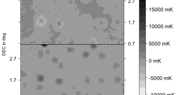
(a) 2 ICs

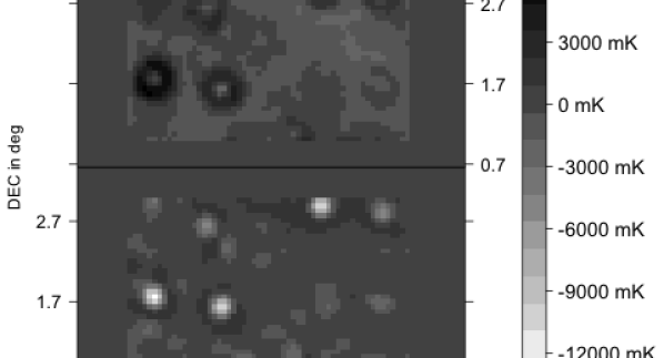
(b) 2 ICs; masked

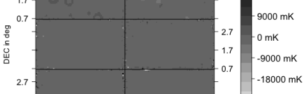
(c) 6 ICs

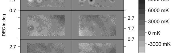
(d) 6 ICs; masked

(e) 10 ICs

(f) 10 ICs; masked

Figure 1: The maps of the independent components identified for sub-dataset A of the 15hr-field, assuming different numbers of ICs. The first column shows the results when analyzing the full field, and the second column displays a masked analysis in which the noise-dominated edges are disregarded.

Furthermore, we examine the residual maps for point source contamination at all frequencies. This can be checked most accurately by summing the residual maps over all frequencies. The instrumental noise and cosmological signal are expected to be close to Gaussian-distributed hence to show no spatial structure when averaging over many frequencies, see e.g. Tegmark & de Oliveira-Costa (1998); Baccigalupi et al. (2000). In Fig. 2, the frequency-combined residual map of the sub-dataset A of the 15hr-field is shown for different numbers of ICs. The analysis of the full field is shown in the first column, and the masked field in the second column. The results from the full maps demonstrate again how the high noise at the edges of the field is not fully modelled by fastica. For the masked analysis with two ICs, as seen in panel (b), the frequency-combined maps contain point-source residuals. These residuals fade out with increasing number of ICs, until they are clearly removed for 10 ICs in panel (f). These tests evidence how fastica is able to model and subtract the strong point sources from the intensity maps using $N_{\rm IC}\geq 6$.

The 1hr-field contains fewer strong point sources, but the observations suffer from inhomogeneous noise properties due to shorter integration times. Although fastica can not effectively model systematic effects with near-Gaussian distributions, the individual sub-datasets exhibit different noise imprints such that their effect on the cross-correlation between the maps should be diminished.

(a) 2 ICs

(b) 2 ICs; masked

(c) 6 ICs

(d) 6 ICs; masked

(e) 10 ICs

(f) 10 ICs; masked

Figure 2: The sum of the temperature residual maps of sub-dataset A of the 15hr-field over all frequency channels. The residual maps after the foreground removal with fastica should only contain noise and 21cm signal. The first and second columns show the sum over the full field, and the analysis in which the edges of the fields are masked, respectively.

4.3 Calibration or instrumental resonance

Some frequency channels of the GBT telescope are sensitive to telescope resonance or RFI. In addition, the calibration of the telescope is a source of error in the amplitude of the measurements. In Fig. 3 the mixing modes $\boldsymbol{a_{i}}$, which give the mixing amplitude per frequency channel, are plotted for an analysis of one dataset of the 15hr-field with 2, 6 and 10 ICs as a function of frequency bin, where bin 0 refers to $f=900\rm MHz$, i.e. $z=0.58$. In a perfect foreground subtraction scenario, each line should represent the flat spectral index of a foreground component. However, instrumental effects such as calibration errors, varying thermal noise, frequency-dependent polarization errors and telescope resonances disturb the flat spectra and allow identification of corrupted data. Around the frequencies 798 MHz and 817 MHz, two known telescope resonances corrupt the measurements and are flagged during the map-making. These channels can be seen as the spikes in panels (a), (b) and (c) of Fig. 3, where we performed fastica on the full data set. After removal of both the contaminated frequency channels and the first few frequency bins which show anomalies due to calibration uncertainties, the resulting mixing modes are shown in panels (d), (e) and (f). One mixing mode spectrum for 2 ICs exhibits two features at high frequency bins which points to a further irregularity in the data due to instrumental effects. In panels (e) and (f), using 6 and 10 ICs, we observe that some modes show high fluctuations around a flat spectrum. These large-amplitude oscillations are due to fastica modelling dominant noise features as ICs. Again, excluding the noisy edges of the field solves this issue, producing the results shown in panels (g), (h) and (i), in which the mixing modes are relatively flat and featureless. We are therefore confident that fastica predominately identifies frequency-dependent foreground components in this case, and we utilize the masked 15hr field with $58\times 33$ pixels in the remainder of this work.

The analysis of the 1hr field exhibits similar improvements when masking the edges, although more fluctuations in the mixing modes are obtained as fastica attempts to model the strong noise features present in these observations. Our default mask of the 1hr-field results in $121\times 53$ pixels.

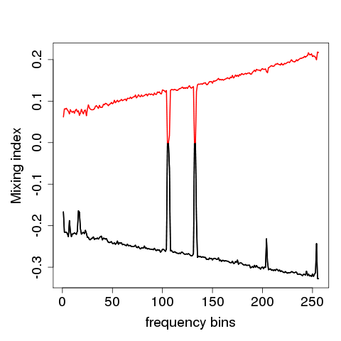
(a) res.; 2 ICs

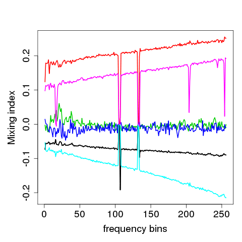
(b) res.; 6 ICs

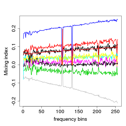
(c) res.; 10 ICs

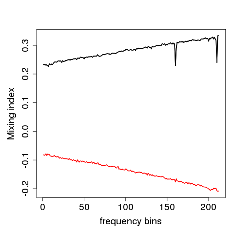
(d) no res.; 2 ICs

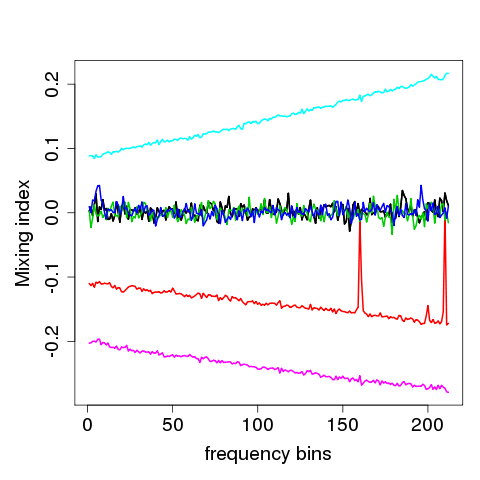
(e) no res.; 6 ICs

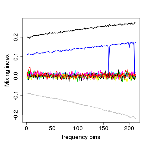
(f) no res.; 10 ICs

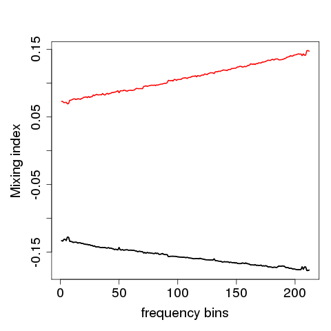
(g) no res.; masked; 2 ICs

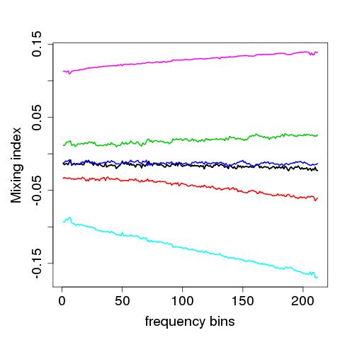
(h) no res.; masked; 6 ICs

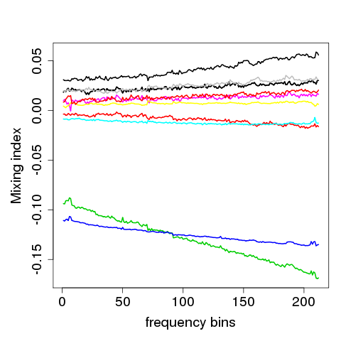
(i) no res.; masked; 10 ICs

Figure 3: The mixing matrix $\mathbf{A}$ as a function of frequency for an analysis of sub-dataset A of the 15hr-field. The three columns show analyses using 2, 6 and 10 ICs, respectively. The first row results from an analysis of the full field. For the analysis shown in the second row, the frequency channels contaminated by instrument resonance, and the first few frequency channels, have been removed. In the third row, the-noise dominated edges of each map are also masked out, which produces a smoothly-varying variation of the mixing matrix with frequency, as expected in a successful foreground subtraction.

4.4 Noise properties

In Fig. 4 we show the standard deviation of the residual maps along the line of sight. For noise-dominated data we expect the standard deviation to be much higher than the amplitude of the sum of all pixels, as can be seen when comparing the standard deviation values with Fig. 2. The structure of the standard deviation maps additionally shows how the noise varies with spatial position. For sub-dataset A of the 15hr-field in Fig. 4, this structure is stable when increasing $N_{\rm IC}$ from 2 to 6 and 10. This suggests that the leakage of noise into the reconstructed Galactic foregrounds is low, and confirms the Gaussian nature of the instrumental noise.

The noise levels of the residuals of the 1hr-field maps are less stable than the 15hr-field with increasing number of ICs, and are dominated by single features with irregular distribution over the map due to the differing observational depth of the pixels. fastica can incorporate some of the strong features as ICs, partially removing the noise systematics. We note that the noise structure of each sub-dataset differs, which prevents contamination of the cross-correlation.

(a) 2 ICs

(b) 6 ICs

(c) 10 ICs

Figure 4: The standard deviation of the temperature residual maps across the frequency channels for sub-dataset A of the 15hr-field, for analyses using 2, 6 and 10 ICs. The standard deviation is unaffected by the number of ICs chosen.

We can access more information about the structure of the data by measuring the 2D power spectra of maps corresponding to individual frequency channels. Following the formalism of Sec. 3, Fourier-transformed temperature maps are calculated as $\tilde{T}_{A}(\vec{k}_{l})=\sum_{j=1}^{N_{pix}}T_{A}(\vec{x}_{j})\exp{(i\vec{k}_{l}\cdot\vec{x}_{j})}$, and the 2D power spectrum is defined as $P_{2D}(\vec{k}_{l})=\mathrm{Re}\{\tilde{T}_{A}(\vec{k}_{l})\tilde{T}_{B}(\vec{k}_{l})^{*}\}$. The noise power spectrum of a frequency map can be estimated via two measures:

• A jack-knife test: the difference of two sub-datasets should only contain thermal noise, since the astrophysical signal remains unchanged with time. We obtain an estimate of the noise power spectrum of one map by calculating the power spectrum of the difference map and dividing it by two. The difference maps also encode systematic errors between the sub-datasets.

• Auto-correlation: the power spectrum of each sub-dataset after the foreground removal should be a proxy for the noise, if it dominates the HI signal.

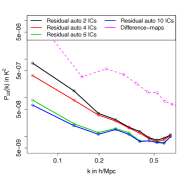
(a) $\nu=838\rm MHz$

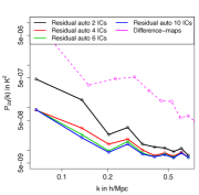
(b) $\nu=806\rm MHz$

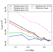
(c) $\nu=775\rm MHz$

Figure 5: 2D auto-power spectra of the residual maps of the 15hr-field for different ICs (solid lines), in comparison to the difference-map power spectrum of the original maps (dashed lines). Each power spectrum is an average of all possible combinations of sub-datasets. These power spectra are a noise approximation of the maps before and after the foreground removal.

(a) Sub-dataset (A - B)

(b) Sub-dataset (A - C)

(c) Sub-dataset (B - C)

Figure 6: The difference maps of the 15hr-field observations for frequency $\nu=869\rm MHz$. The difference maps exhibit spatial structure due to systematic errors in the sub-datasets.

In Fig. 5 we show a few examples of the 2D power spectra of the difference maps and the auto-correlations of the 15hr-field, where we averaged over all possible combinations of sub-datasets. It can be seen that the difference-map correlations contain more power than the auto-correlations. This can be explained in terms of the spatial structure of the difference maps, shown in Fig. 6. The difference maps show a clear structure at the position of the point sources, produced by instrumental effects which correlate with the amplitude of signal such as calibration errors, pointing offsets and thermal noise. The amplitude of this systematic contribution does not depend on frequency. fastica models the point sources in each sub-dataset independently, hence can remove these systematic effects. The analysis of the 1hr-field shows similar behaviour.

4.5 Residual-foreground correlation

We can also evaluate the foreground removal by considering the 2D cross-power spectra between different frequency maps. In the following plots, we show two kinds of correlations:

• The cross-correlation of the residual maps from different sub-datasets. This cross-correlation should be driven by the cosmological signal, since the noise is uncorrelated between sub-datasets. However, it could also be produced by residual foreground contamination.

• The cross-correlation of the residuals and the reconstructed foreground maps. Such a signal could be produced if the foregrounds are insufficiently modelled and contaminate the residuals, or if the ICs contain instrumental noise or cosmological signal.

In Fig. 7 we display examples of these 2D power spectra, analyzing the full field in the first column and the masked field in the second column, for a series of stacks of 20 frequency channels. Since the maps are dominated by thermal noise, the noise decreases as $1/\sqrt{N}$ when adding $N$ frequency channels.

The amplitudes of the cross-correlations are proportional to the product of mean temperatures of the two input maps. In order to compare the cross-correlation of foreground and residuals to the correlation of residual maps we need to normalize the amplitude, for which we use the standard deviations of the respective maps.

In the first column, the figures show the results of the flawed fastica decomposition which insufficiently removes the point sources of the foregrounds, as seen in the stacked maps in Fig. 2. The solid lines show a similar behaviour for different number of ICs and frequencies, indicating a correlation between foregrounds and residuals. In the second column the masked results, which are clean of point source contamination, are shown. The cross-correlation of foreground and residuals are relatively random-distributed and are an indication that the data is dominated by statistical noise not systematic foregrounds. The dashed lines in all figures are the residual correlation between all combinations of sub-datasets. These converge for increasing number of ICs, confirming the results of the successful foreground removal of previous tests and demonstrating that our results do not sensitively depend on the number of ICs chosen. The cross-correlation of the residuals and foregrounds of the 1hr-field show similar behaviour.

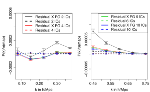
(a) Frequency bins 80-99; no mask

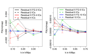
(b) Frequency bins 80-99; edges masked

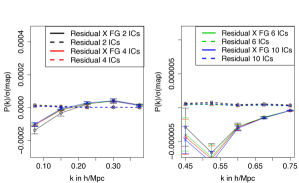
(c) Frequency bins 140-159; no mask

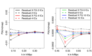
(d) Frequency bins 140-159; edges masked

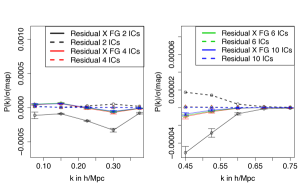
(e) Frequency bins 220-239; no mask

(f) Frequency bins 220-239; edges masked

Figure 7: The 2D cross-power spectra between reconstructed foregrounds and residuals of the 15hr-field, marked as the solid lines for different numbers of ICs with different colors. The dashed lines represent the residual power spectrum between sub-datasets. Each panel shows the 2D power spectrum with different scales for large and small wavenumbers $k$. The correlations in each row are estimated over three frequency ranges, each containing 20 frequency bins. The first column of 2 panels is for a full-field analysis, and the second column shows results for the masked field.

5 3D Power Spectrum Results

5.1 Auto-Correlations

In this section we present the results of the 3D power spectrum estimation from the GBT intensity maps. We consider three different strategies for estimating errors in the power spectrum measurements, and compare these in Fig. 8:

• We use the auto-correlations of the residual maps as a proxy for the noise power spectrum in Eq. 4 (solid error bar).

• We use the power spectrum of the difference of the maps, divided by 2, as a proxy for the noise power spectrum in Eq. 4 (dashed error bar).

• We calculate the standard deviation of the 6 sub-dataset cross-power spectra used in the analysis, and divide it by $\sqrt{6}$ to produce an error in the mean (dotted error bar).

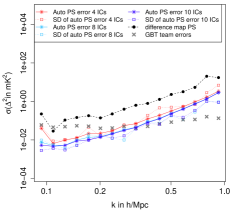
(a) 15hr-field

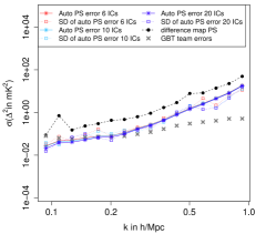
(b) 1hr-field

Figure 8: Different estimates of the error in the 3D power spectrum measurement are shown for different numbers of ICs, for the 15hr-field and 1hr-field. The black dashed line is the error estimate based on the difference maps. The solid coloured line shows the error based on the auto-correlations of the sub-dataset, and the dotted coloured line represents the standard deviation of the cross-power spectrum measurements between the sub-datasets. The error estimates of the SW13 analysis are marked by grey crosses.

The error based on the noise estimate from the difference maps (black dashed line) is higher than the other two error estimates. We believe that this provides an upper limit on the error in the measurements since it includes systematic effects correlated with the foregrounds, which fastica partially subtracts from the data. The noise estimate from the auto-correlation gives a better approximation to the errors in the foreground-subtracted measurements.

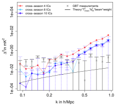
(a) 15hr-field

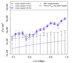
(b) 1hr-field

Figure 9: The 3D intensity mapping cross-power spectrum between sub-datasets of the 15hr field data (left-hand panel) and 1hr field (right-hand panel), showing the different error estimates from Fig. 8 using the respective line styles. The measurements from SW13 are marked by grey crosses. The black line shows the theoretical model power spectrum convolved with the window functions assuming $\Omega_{\rm HI}b_{\rm HI}=0.43\cdot 10^{-3}$.

In Fig. 9, we present the intensity mapping power spectrum estimates for different numbers of ICs used for the foreground subtraction, in comparison with the results published by SW13, which are marked by grey symbols. The estimates are the average of all possible combinations of the cross-power spectra between the 4 sub-datasets, showing the different error estimates from Fig. 8 with their respective line styles. The power spectra have all been corrected for the telescope beam, using a constant beam model with $\theta_{\rm FWHM}=0.44\deg$ for the SW13 data points, and a frequency-dependent beam for the fastica measurements.

The power spectra converge with increasing number of ICs, showing that fastica is a robust method to remove the non-Gaussian foregrounds. In Fig. 9(a), we see that our measured power spectra in both fields are in reasonable agreement with the results of SW13 on large scales with $k<0.2h\rm{Mpc}^{-1}$, but diverge for smaller scales. The power spectrum amplitude of the 1hr-field is higher than the 15hr field, due to some residual foregrounds and significant instrumental systematics in the 1hr-field maps. The GBT measurements are corrected for signal loss by an anisotropic transfer function $T(k_{\perp},k_{\parallel})$, as described by Switzer et al. (2015). The power spectrum of the fastica-cleaned data does not require any corrections by a transfer function since the signal loss is negligible, as shown by Wolz et al. (2014).

The high amplitude of the intensity mapping power spectra measured by fastica on smaller scales is driven by its conservative approach to foreground subtraction. This is in contrast to the SVD method, which removes modes with high amplitudes regardless of their statistical properties. This comparison shows that fastica provides a robust upper limit on the foreground removal, while SVD could provide a lower limit on the removable foreground modes. Both methods have been shown to perform well in a simulated environment (Alonso et al., 2015). However, in the presence of high instrumental noise and systematics, the foreground removal methodology can lead to significant differences. fastica succeeds in removing resolved point sources and diffuse frequency-dependent foregrounds dominating on large scales. However, it is not equipped to mitigate systematics on smaller scales dominated by thermal noise. The SVD approach removes modes on all scales, but is prone to HI signal loss. We believe that the application of both methods is a useful approach when investigating foregrounds and systematics of intensity mapping data.

In general, the auto-correlations of the 15hr and 1hr fields are high compared to the theoretical prediction. This discrepancy could be explained in several ways. Systematics leftover from the foreground subtraction could boost the amplitude of the power spectrum, and additional power could be added to the 21cm signal by fluctuations introduced by polarization leakage. Finally, a different predicted amplitude could be produced by changing the value of $\Omega_{\rm HI}b_{\rm HI}$.

5.2 Cross-Correlation with WiggleZ

The cross-power spectra of the intensity maps with the WiggleZ galaxy survey for both fields is shown in Fig. 10, for a range of different numbers of ICs. The errors in this figure are given by the standard deviation of the estimates between the sub-datasets, and the empty symbols mark negative correlations. The cross-power spectra converge with increasing number of ICs for both fields, verifying that fastica does not subtract 21cmsignal from the data.

In Fig. 11 we show the cross-correlation for both the 15hr and 1hr fields, using 10 and 20 ICs respectively, in comparison with the results of MA13, which are marked with blue and green shaded areas. Two measurement errors are shown: the standard deviation of the estimates between the sub-datasets (as the solid lines) and the theoretical expectation computed using Equ. 5 (as the dashed lines), which respectively provide an upper and lower limit of the measurement errors. Negative cross-correlations are again indicated by empty symbols. Fig.11(a) demonstrates that our estimates generally agree with the previous findings.

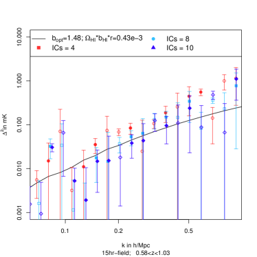
(a) 15hr-field

(b) 1hr-field

Figure 10: The 3D cross-power spectrum of the GBT intensity maps and WiggleZ galaxies, for foreground subtraction with different numbers of ICs. Results are shown for the 15hr-field in the left panel and the 1hr-field in the right panel. The black lines are the theoretical model convolved with the respective window functions assuming $\Omega_{\rm HI}b_{\rm HI}=0.43\cdot 10^{-3}$.

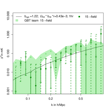
(a) 10 ICs; 15hr-field

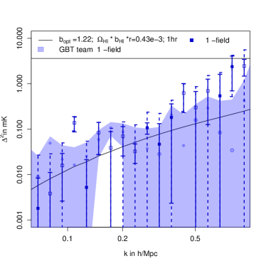
(b) 20 ICs; 1hr-field

Figure 11: The 3D cross-power spectrum of the GBT intensity maps and WiggleZ galaxies, for the 15hr field (using foreground subtraction with 10 ICs) in the left-hand panel, and for the 1hr field (using 20 ICs) in the right-hand panel. The results of MA13 are marked by the shaded areas. The black lines are the theoretical model convolved with the respective window functions assuming $\Omega_{\rm HI}b_{\rm HI}=0.43\cdot 10^{-3}$. The solid error bars are given by the standard deviation between sub-datasets and the dashed error bars using Equ. 5.

6 Conclusions

In this study we present a thorough analysis of two intensity-mapping fields observed by the GBT, previously analysed by Masui et al. (2013) and Switzer et al. (2013). Our pipeline includes a Fourier-based, weighted power spectrum estimator for auto-correlations and cross-correlations with galaxy surveys. We remove the diffuse Galactic foregrounds and point source contamination with fastica, which separates components based on a measure of their non-Gaussianity. The subtraction fidelity and systematic errors are investigated for analyses with different numbers of ICs, showing that the residual maps converge and the results are not dependent on this choice. We explore different masking of the maps to reduce strong noise contamination at the edges of the fields. We confirm that fastica is well-suited for subtracting the Galactic and non-Galactic foregrounds from intensity mapping data since, by construction, it does not remove Gaussian 21cm signal but can not prevent from removing the possibly non-Gaussian 21cm signal.

The auto-correlation of the residual intensity maps from fastica has a higher amplitude than the previous measurements by MA13 and SW13. This is because fastica is a conservative foreground removal technique compared to the SVD method. Both techniques measure auto-correlation power significantly above our current best guess of the cosmological signal, indicating severe systematic contamination in the current datasets. The cross-power spectrum between the intensity map and the WiggleZ galaxy survey converges with increasing number of ICs, and is in reasonable agreement with the measurements of MA13.

We conclude that SVD and fastica serve as complementary tools for exploring the systematics and quality of foreground removal in noise-dominated intensity mapping datasets. In future work, we are planning to combine both techniques in order to exploit their individual advantages in the data reduction.

References

- Alonso et al. (2015) Alonso D., Bull P., Ferreira P. G., Santos M. G., 2015, MNRAS, 447, 400
- Ansari et al. (2008) Ansari R., Le Goff J. ., Magneville C., Moniez M., Palanque-Delabrouille N., Rich J., Ruhlmann-Kleider V., Yèche C., 2008, ArXiv e-prints 0807.3614
- Baccigalupi et al. (2000) Baccigalupi C., Bedini L., Burigana C., De Zotti G., Farusi A., Maino D., Maris M., Perrotta F., Salerno E., Toffolatti L., Tonazzini A., 2000, MNRAS, 318, 769
- Battye et al. (2004) Battye R. A., Davies R. D., Weller J., 2004, MNRAS, 355, 1339
- Blake et al. (2013) Blake C., Baldry I. K., Bland-Hawthorn J., Christodoulou L., Colless M., Conselice C., Driver S. P., Hopkins A. M., Liske J., Loveday J., Norberg P., Peacock J. A., Poole G. B., Robotham A. S. G., 2013, MNRAS, 436, 3089
- Blake et al. (2010) Blake C., Brough S., Colless M., Couch W., Croom S., Davis T., Drinkwater M. J., Forster K., Glazebrook K., Jelliffe B., et al., 2010, MNRAS, 406, 803
- Bull et al. (2015) Bull P., Ferreira P. G., Patel P., Santos M. G., 2015, ApJ, 803, 21
- Chang et al. (2010) Chang T.-C., Pen U.-L., Bandura K., Peterson J. B., 2010, Nature, 466, 463
- Chang et al. (2008) Chang T.-C., Pen U.-L., Peterson J. B., McDonald P., 2008, Phys.Rev.Lett., 100, 091303
- Chapman et al. (2012) Chapman E., Abdalla F. B., Harker G., Jelic V., Labropoulos P., et al., 2012, MNRAS, 423, 2518
- Drinkwater et al. (2010) Drinkwater M. J., Jurek R. J., Blake C., Woods D., Pimbblet K. A., Glazebrook K., Sharp R., Pracy M. B., Brough S., Colless M., et al., 2010, MNRAS, 401, 1429
- Eisenstein et al. (2005) Eisenstein D. J., et al., 2005, ApJ, 633, 560
- Gong et al. (2011) Gong Y., Chen X., Silva M., Cooray A., Santos M. G., 2011, ApJ, 740, L20
- Hyvärinen (1999) Hyvärinen A., 1999, IEEE Transactions on Neural Networks, 10, 626
- Lewis et al. (2000) Lewis A., Challinor A., Lasenby A., 2000, Astrophys. J., 538, 473
- Lidz et al. (2011) Lidz A., Furlanetto S. R., Oh S. P., Aguirre J., Chang T.-C., Doré O., Pritchard J. R., 2011, ApJ, 741, 70
- Maino et al. (2002) Maino D., Farusi A., Baccigalupi C., Perrotta F., Banday A. J., Bedini L., Burigana C., De Zotti G., Górski K. M., Salerno E., 2002, MNRAS, 334, 53
- Masui et al. (2013) Masui K. W., Switzer E. R., Banavar N. andBandura K., Blake C., Calin L.-M., Chang T.-C., Chen X., Li Y.-C., Liao Y.-W., Natarajan A., Pen U.-L., Peterson J. B., Shaw J. R., Voytek T. C., 2013, ApJ, 763, L20
- Olivari et al. (2016) Olivari L. C., Remazeilles M., Dickinson C., 2016, MNRAS, 456
- Percival et al. (2007) Percival W. J., Cole S., Eisenstein D. J., Nichol R. C., Peacock J. A., et al., 2007, MNRAS, 381, 1053
- Percival et al. (2010) Percival W. J., Reid B. A., Eisenstein D. J., Bahcall N. A., Budavari T., Frieman J. A., Fukugita M., Gunn J. E., Ivezić Ž., Knapp G. R., Kron R. G., Loveday J., Lupton R. H., 2010, MNRAS, 401, 2148
- Peterson & Suarez (2012) Peterson J. B., Suarez E., 2012, ArXiv e-prints 1206.0143
- Planck Collaboration X, (2015) Planck Collaboration X, 2015, ArXiv e-prints 1502.01588
- Planck Collaboration XIII (2015) Planck Collaboration XIII 2015, ArXiv e-prints 1502.01589
- Planck Collaboration XXV, (2015) Planck Collaboration XXV, 2015, ArXiv e-prints 1506.06660
- Pullen et al. (2014) Pullen A. R., Doré O., Bock J., 2014, ApJ, 786, 111
- Shaw et al. (2014) Shaw J. R., Sigurdson K., Pen U.-L., Stebbins A., Sitwell M., 2014, ApJ, 781, 57
- Shaw et al. (2015) Shaw J. R., Sigurdson K., Sitwell M., Stebbins A., Pen U.-L., 2015, Phys. Rev. D, 91, 083514
- Switzer et al. (2015) Switzer E. R., Chang T.-C., Masui K. W., Pen U.-L., Voytek T. C., 2015, ApJ, 815, 51
- Switzer et al. (2013) Switzer E. R., Masui K. W., Bandura K., Calin L.-M., Chang T.-C., Chen X.-L., Li Y.-C., Liao Y.-W., Natarajan A., Pen U.-L., Peterson J. B., Shaw J. R., Voytek T. C., 2013, MNRAS, 434, L46
- Tegmark (1997) Tegmark M., 1997, ApJ, 480, L87
- Tegmark & de Oliveira-Costa (1998) Tegmark M., de Oliveira-Costa A., 1998, ApJ, 500, L83
- Tegmark et al. (2004) Tegmark M., et al., 2004, Astrophys. J., 606, 702
- Vujanovic et al. (2009) Vujanovic G., Staveley-Smith L., Pen U.-L., Chang T.-C., Peterson J., 2009, ATNF Proposal, p. 2491
- White et al. (2009) White M., Song Y.-S., Percival W. J., 2009, MNRAS, 397, 1348
- Wolz et al. (2014) Wolz L., Abdalla F. B., Blake C., Shaw J. R., Chapman E., Rawlings S., 2014, Mon. Not. Roy. Astron. Soc., 441, 3271
- Wyithe et al. (2008) Wyithe J. S. B., Loeb A., Geil P. M., 2008, MNRAS, 383, 1195
- Zhang et al. (2016) Zhang L., Bunn E. F., Karakci A., Korotkov A., Sutter P. M., Timbie P. T., Tucker G. S., Wandelt B. D., 2016, ApJS, 222, 3