Introduction to low-momentum effective interactions with
Brown-Rho scaling and three-nucleon forces

Abstract

Model-space effective interactions $V_{eff}$ derived from free-space nucleon-nucleon interactions $V_{NN}$ are reviewed. We employ a double decimation approach: first we extract a low-momentum interaction $V_{low-k}$ from $V_{NN}$ using a $T$-matrix equivalence decimation method. Then $V_{eff}$ is obtained from $V_{low-k}$ by way of a folded-diagram effective interaction method. For decimation momentum $\Lambda\simeq 2fm^{-1}$, the $V_{low-k}$ interactions derived from different realistic $V_{NN}$ models are nearly model independent, and so are the resulting shell-model effective interactions. For nucleons in a low-density nuclear medium like valence nucleons near the nuclear surface, such effective interactions derived from free-space $V_{NN}$ are satisfactory in reproducing experimental nuclear properties. But it is not so for nucleons in a nuclear medium with density near or beyond nuclear matter saturation density. In this case it may be necessary to include the effects from Brown-Rho (BR) scaling of hadrons and/or three-nucleon forces $V_{3N}$, effectively changing the free-space $V_{NN}$ into a density-dependent one. The density-dependent effects from BR scaling and $V_{3N}$ are compared with those from empirical Skyrme effective interactions.

1 Introduction

In treating nuclear many-body problems, one can often reduce the “full” many-body problem to a much smaller and more manageable problem, referred to as a model-space problem. In so doing, an important step is to determine the model-space effective interaction $V_{eff}$. In this paper, we would like to present an introductory and pedagogical review of this topic, especially the derivation of $V_{eff}$ from realistic meson-exchange nucleon-nucleon interactions.

Many-body problems are difficult as we are all aware of. They are particularly so, when A, the number of particles in the system, is large. In fact a many-body problem with A=3 is already a very hard problem. In the real world, A is usually much larger. For example, A=18 when the nucleus ${}^{18}O$ is treated as an 18-nucleon problem. It becomes an A=54 problem if it is treated as composed of 54 quarks. So the complexity of the problem depends largely on how we look at the problem, or, more precisely, it depends on what is our “model space” within which we are making our observations.

Let us consider the nucleus ${}^{18}O$ as an example; it is a system of 18 nucleons. The nuclear shell model has been the most successful model for nuclear structure. This model is in fact a model-space approach. The wave functions $\Psi_{n}$ of this nucleus consists of, in principle, shell-model wave functions $|2p0h\rangle$, $|3p1h\rangle$, …. and $|18p16h\rangle$; $p$ and $h$ denoting particles and holes with respect to a closed ${}^{16}O$ core. The dimension of this full shell-model space is practically “infinite”. For actual calculations, some truncation or renormalization of the full-space problem is indispensible. To describe the low-energy properties of this nucleus, it may not be necessary to consider all these wave-function components; it may be sufficient to include just some low-energy parts of them. This is actually the approach commonly used in the shell-model description of ${}^{18}O$, where this nucleus is treated as composed of two valence neutrons in the 0d1s shell outside a closed ${}^{16}O$ core. Denoting this restricted model space as P, the Hamiltonian for this nucleus is $P(H_{0}+V_{eff})P$ where $V_{eff}$ is the effective interaction and $H_{0}$ denotes the single-particle (sp) Hamiltonian.

Nucleus	Experimental	Calculated
${}^{41}Ca$	8.36	8.38
${}^{42}Ca$	19.83	19.86
${}^{43}Ca$	27.75	27.78
${}^{44}Ca$	38.89	38.80
${}^{45}Ca$	46.31	46.26
${}^{46}Ca$	56.72	56.82
${}^{47}Ca$		63.81
${}^{48}Ca$	73.95	73.93

Table 1: Binding energies of Ca isotopes in MeV given by Talmi’s $(0f_{7/2})^{n}$ model.[1]

In such model-space approaches, an important step is to employ some empirically determined effective interactions $V_{eff}$. And indeed such approaches have been very successful. To illustrate this, let us consider the pioneering work of Talmi [1] on the calcium isotopes ${}^{41}Ca-{{}^{48}Ca}$. In this work these isotopes were treated as composed of $n$ valence neutrons in the $0f_{7/2}$ shell outside an inert ${}^{40}Ca$ core. In other words, a restricted model space of $(0f_{7/2})^{n}$ is employed. For this model space, $V_{eff}$ can be expressed in terms of three parameters. In fact the ground-state energies are given by a very simple formula

$$\langle(0f_{7/2})^{n}|H_{eff}|(0f_{7/2})^{n}\rangle=nC+\frac{n(n-1)}{2}\alpha+[\frac{1}{2}n]\beta$$ (1)

where $[\frac{1}{2}n]$ is the step function equal to $\frac{n}{2}$ if $n$=even, and $\frac{n-1}{2}$ if $n$= odd. The parameters $C$, $\alpha$ and $\beta$ can be determined by fitting the experimental energies. The optimum values, in MeV, are determined as

$$C=8.38\pm 0.05,~{}~{}\alpha=-0.21\pm 0.01,~{}~{}\beta=3.33\pm 0.12.$$

The binding energies given by these parameters are compared with experiments in Table 1. As seen the agreement is astonishingly excellent. The term $C$ is just the neutron sp energy which can be extracted from the experimental binding energies of ${}^{41}Ca$ and ${}^{40}Ca$. We note that the optimum value of $C$ is practically the same as the experimental sp energy (8.38 vs 8.36). $C$ is actually not a parameter; it is the experimental sp energy. Thus in this model space approach, there are only two parameters, $\alpha$ and $\beta$, which characterize the effective interaction $V_{eff}$. The above example strongly indicates the success of the model-space approach: by confining the nucleons to a small (manageable) space and treating $V_{eff}$ as composed of adjustable parameters, experimental results can indeed be quite satisfactorily reproduced.

Figure 1: Comparison of the ${}^{1}S_{0}-{{}^{1}S_{0}}$ diagonal momentum-space matrix elements $V(k,k)$ of Paris [6], CD-Bonn [8], Argonne [9], Nijmegen [10] and Idaho [11] potentials.

Figure 2: Same as Fig. 1 except for the ${}^{3}S_{1}-{{}^{3}S_{1}}$ channel.

A challenging task is to see if we can derive microscopically the empirical $V_{eff}$ from an underlying nucleon-nucleon (NN) interaction. Since the early works of Brown and Kuo [2, 3], this question has been rather extensively studied (see e.g. Refs. [4, 5] and references quoted therein). In microscopic nuclear structure calculations starting from $V_{NN}$, a well-known ambiguity has been the choice of NN potential. There are a number of successful models for $V_{NN}$, such as the Paris [6], Bonn [7], CD-Bonn [8], Argonne V18 [9], Nijmegen [10] and the chiral Idaho [11] potentials. A common feature of these potentials is that they all reproduce the empirical deuteron properties and low-energy phase shifts very accurately. But, as illustrated in Figs. 1 and 2, these potentials are in fact significantly different from each other in the momentum representation. This has been a situation of much concern. Certainly we would like to have a “unique” NN potential (like the Coulomb potential between two electric charges). As seen, the above potentials are not ‘unique’. Which of them is the ‘right’ NN interaction? We shall make an effort addressing this question.

The present paper is organized as follows. In section II we shall describe in some detail a $\hat{Q}$-box folded-diagram expansion for the model-space effective interaction $V_{eff}$ for valence nuclei such as ${}^{18}O$ and ${}^{19}O$ confined within a model space $P$. In this formalism the effective Hamiltonian is of the form $PH_{eff}P=P(H_{0}^{expt}+V_{eff})P$ where the sp Hamiltonian $H_{0}^{expt}$ is obtained from the experimental energies of nuclei with one valence nucleon such as ${}^{17}O$. The general structure of this formalism is compared with the Talmi approach described earlier. Methods for summing up the folded-diagram series for degenerate and non-degenerate, such as two-major-shell, model spaces are discussed, and with them the present framework can be used to calculate the model-space $V_{eff}$ from input nucleon-nucleon interactions.

In section III we shall review a $T$-matrix equivalence approach for deriving the low-momentum NN interaction $V_{low-k}$ by integrating, or decimating, out the high-momentum modes of the input interaction. Momentum space matrix elements of $V_{low-k}$ calculated from different $V_{NN}$ potentials are compared. The counter terms generated by the above decimation are discussed. The $V_{low-k}$ interaction so constructed is non-Hermitian and transformation methods for making it Hermitian are described. In section IV we shall describe Brown-Rho (BR) scaling, three-nucleon forces, and the density-dependent effects generated by them. Applications to nuclear structure, nuclear matter and neutron stars will be reported. A summary and discussion will be presented in section V.

2 Folded-diagram expansion for effective interactions $V_{eff}$

In this section we shall describe some details of the folded-diagram expansion for the shell-model effective interaction $V_{eff}$ [12, 13]. Let us first discuss a similarity between this expansion and that for the ground-state energy of a closed-shell (or filled Fermi-sea) system such as ${}^{16}O$ (or nuclear matter). Consider the nuclear matter case, whose true and unperturbed ground-state energies are denoted by $E_{0}$ and $W_{0}$ respectively. The ground-state energy shift $\Delta E_{0}=E_{0}-W_{0}$ is given by the Goldstone linked-diagram expansion [12, 13, 14], namely the sum of all the linked diagrams, as shown in Fig. 3. Here diagram (a) is the lowest order such diagram (usually referred to as the Hartree-Fock interaction diagram). Diagram (b) is a particle-particle ladder diagram having repeated interactions between a pair of particle lines. Diagram (c) is a ring diagram (see e.g., Ref. [15, 16]) with both particle-particle and hole-hole interactions.

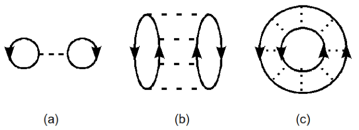
Figure 3: Sample diagrams contained in the Goldstone linked diagram expansion for the ground-state energy shift $\Delta E_{0}$. Each dashed line represents a nuclear interaction vertex.

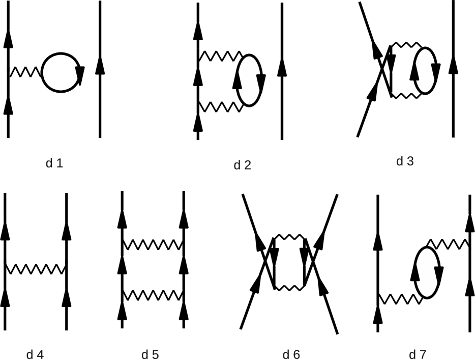
Figure 4: Low-order diagrams belonging to the $\hat{Q}$-box for ${}^{18}O$. Note that the intermediate states between two successive vertices must be outside the chosen model space as discussed later.

The Goldstone expansion provides a framework for calculating, for example, the ground-state energy of ${}^{16}O$. What would then be the corresponding framework for calculating the low-lying $0^{+}$ states of ${}^{18}O$? It is here the folded-diagram expansion comes in. This expansion provides a framework for such and similar calculations. It is a generalization of the Goldstone expansion to systems with valence particles confined to a multi-dimensional model space. Consider again ${}^{18}O$ as an example. This nucleus has two valence neutrons, and as shown in Fig. 4 the diagrams of its effective interaction all have two valence lines in their initial and final states. (Note that the initial and final states of the Goldstone diagrams as shown in Fig. 3 are both vacuum.) In a shell-model calculation of the low-lying $0^{+}$ states of ${}^{18}O$, one usually treats it as two valence neutrons confined in the $0d1s$ shell with an effective Hamiltonian $H_{eff}=H_{0}+V_{eff}$. In this case the $V_{eff}$ for the valence neutrons is a matrix of dimension three. One obtains both the ground- and excited-state energies of the system by solving a matrix equation involving $V_{eff}$. (In the Goldstone expansion, the ground-state energy is given by the sum of all the linked diagrams.) The purpose of the folded-diagram expansion [12, 13] is to provide a microscopic framework to derive such $V_{eff}$ from an underlying $V_{NN}$ potential.

The nuclear many-body Schroedinger equation may be written as

$$H\Psi_{n}(1,2,..A) = E_{n}(1,2,..A)\Psi_{n}(1,2,...A);$$

$$H = T+V_{NN}$$ (2)

where $T$ denotes the kinetic energy. To define a convenient sp basis, we introduce an auxiliary potential $U$ and rewrite $H$ as

$$H=H_{0}+H_{1};~{}H_{0}=T+U,~{}H_{1}=V_{NN}-U.$$ (3)

The choice of $U$ is very important, and in principle we can use any $U$ of our choice. However, an optimized choice is to have a $U$ such that $H_{1}$ becomes “small”. In this way $H_{1}$ may be treated as a perturbation. We denote the sp wave functions and energies defined by $H_{0}$ as $\phi$ and $\epsilon$, namely $H_{0}\phi_{n}=\epsilon_{n}\phi_{n}$.

The many-body problem as specified by Eq. (2) is in general very difficult. It has a large number of solutions. In fact we may not need to know all of them; perhaps only a few of them are of physical interest and we should just calculate these few solutions. Thus we aim at the reduction of Eq. (2) to a model-space equation of the form

$$PH_{eff}P\Psi_{m}=E_{m}P\Psi_{m};~{}m=1,\cdots,d$$ (4)

where $P$ is the model-space projection operator defined by

$$P=\sum_{n=1,d}|\Phi_{n}\rangle\langle\Phi_{n}|.$$ (5)

Here $\Phi$ is a Slater determinant composed of the sp wave functions $\phi$. The above equation reproduces only $d$ solutions of Eq. (2). Furthermore, it does not give the complete wave function. It gives only the projection of the whole wave function onto the model space ($P$) of one’s choice.

The main idea behind Eq. (4) is to have a smaller, and hopefully more manageable, many-body problem than the original problem of Eq. (2). This approach is useful if the effective Hamiltonian can be obtained without too much difficulty. Hence the question now is how to derive $H_{eff}$, or how to derive the effective interaction $V_{eff}$ which is related to $H_{eff}$ by

$$H_{eff}=H_{0}+V_{eff}.$$ (6)

There are various ways to obtain $H_{eff}$ or $V_{eff}$. Let us first describe briefly the Feshbach [17] formulation of the model-space effective Hamiltonian. In matrix form Eq. (2) is written as

$$\left(\begin{array}[]{cc}PHP&PHQ\\ QHP&QHQ\end{array}\right)\left(\begin{array}[]{c}P\Psi\\ Q\Psi\end{array}\right)=E\left(\begin{array}[]{c}P\Psi\\ Q\Psi\end{array}\right)$$ (13)

where $Q$ is the complement of $P$, namely $Q=1-P$. We can readily eliminate $Q\Psi$, obtaining a $P$-space equation

$$H_{eff}(E_{n})P\Psi_{n}=E_{n}P\Psi_{n}$$ (14)

with

$$H_{eff}(E_{n})=PHP+PHQ\frac{1}{E_{n}-QHQ}QHP.$$ (15)

This is an interesting result. We see that now we only need to deal with an equation which is entirely contained in the $P$ space. However, a significant drawback here is that the effective Hamiltonian is dependent on the eigenvalue $E_{n}$. In other words, we need to use different effective interactions for different eigenstates. This feature is clearly not convenient or desirable.

The folded-diagram method has been developed with the purpose of providing an energy-independent (namely independent of the energy eigenvalue $E_{n}$) model-space effective interaction. There have been several studies of the folded-diagram method [12, 13, 18, 19, 20, 21]. Among them, the time-dependent formulation of Kuo, Lee and Ratcliff (KLR) [12, 13] is particularly suitable for shell-model calculations. It provides a formal framework for reducing the full-space many-body problem, as shown by Eq. (2), to a model-space one of the form

$$PH_{eff}P\Psi_{m} = (E_{m}-E_{0}^{core})P\Psi_{m};$$

$$PH_{eff}P = P[H_{0}^{expt}+V_{eff}]P$$ (16)

where $m=1,...,d$; $d$ being the dimension of the model space. Note that this equation calculates the energy difference between neighboring nuclei. For example, $E_{m}$ is the energy of ${}^{19}O$ and $E_{0}^{core}$ is the ground-state energy of ${}^{16}O$. In addition, $H_{0}^{expt}$ is the sp energy part which is extracted from experimental energy differences between neighboring nuclei such as ${}^{17}O$ and ${}^{16}O$. The above $H_{eff}$ is of the same form as the one commonly used in shell-model calculations (such as the calculation of the $Ca$ isotopes mentioned earlier), except that here $V_{eff}$ is derived from the nucleon-nucleon interaction $V_{NN}$ whereas in empirical shell-model calculations it is determined empirically by fitting experimental data. The folded-diagram method has been applied to a wide range of nuclear structure calculations using realistic NN interactions [4, 5, 22].

In deriving $V_{eff}$ microscopically, we shall employ the time evolution operator $U(t,t^{\prime})=exp[-iH(t-t^{\prime})]$ in the complex-time limit, namely

$$\lim_{t^{\prime}\rightarrow-\infty(\epsilon)}\equiv\lim_{\epsilon\rightarrow 0^{+}}\lim_{t^{\prime}\rightarrow-\infty(1-i\epsilon)}$$ (17)

In this limit it can be shown that we can construct, starting from a model-space parent state $\rho_{i}$, the lowest eigenstate $\Psi_{i}$ of the true Hamiltonian with $\langle\rho_{i}|\Psi_{i}\rangle\neq 0$, namely

$$\lim_{t^{\prime}\rightarrow-\infty(\epsilon)}\frac{U(0,t^{\prime})|\rho_{i}\rangle}{\langle\rho_{i}|U(0,t^{\prime})|\rho_{i}\rangle}=\frac{|\Psi_{i}\rangle}{\langle\rho_{i}|\Psi_{i}\rangle},$$ (18)

where the parent state is a linear combination of the model-space basis vectors $\Phi_{k}$,

$$|\rho_{\lambda}\rangle=\sum_{k=1,d}C_{\lambda,k}|\Phi_{k}\rangle,$$ (19)

$d$ being the dimension of the model space. When $P\Psi_{\lambda}$ for $\lambda=1,...,d$ are linearly independent, the $C_{\lambda,k}$ coefficients can satisfy

$$\langle\rho_{\lambda}|\Psi_{\mu}\rangle=\langle\rho_{\lambda}|P\Psi_{\mu}\rangle=0,$$ (20)

for $\lambda\neq\mu;~{}\lambda,\mu=1,...,d$. Then we have

$$H\frac{U(0,t^{\prime})|\rho_{\lambda}\rangle}{\langle\rho_{\lambda}|U(0,t^{\prime})|\rho_{\lambda}\rangle}=E_{\lambda}\frac{U(0,t^{\prime})|\rho_{\lambda}\rangle}{\langle\rho_{\lambda}|U(0,t^{\prime})|\rho_{\lambda}\rangle},$$ (21)

where $\lambda=1,...,d$ with the complex-time limit $t^{\prime}\rightarrow-\infty(\epsilon)$ understood.

Eq. (15) is the basic equation for deriving the model-space effective interaction $V_{eff}$ using a folded-diagram factorization procedure, which has been given in detail in [12, 13]. Here we shall just outline some basic features of the procedure such as “what is a folded diagram”.

In the interaction representation, we have

$$U(t,t^{{}^{\prime}}) = 1+\sum_{n=1}^{\infty}(-i)^{n}\int_{t^{{}^{\prime}}}^{t}dt_{1}\int_{t^{{}^{\prime}}}^{t_{1}}dt_{2}\cdots$$ (22)

$$\int_{t^{{}^{\prime}}}^{t_{n-1}}dt_{n}H_{1}(t_{1})H_{1}(t_{2})\cdots H_{1}(t_{n}).$$

Consider the wave function generated by the operation $U(0,-\infty)|\Phi_{\alpha\beta}\rangle$ where $|\Phi_{\alpha\beta}\rangle$ is a two-particle state defined by $a^{+}_{\alpha}a^{+}_{\beta}|0\rangle$. Here the $a^{+}$’s are the sp creation operators and $|0\rangle$ is the vacuum state. As indicated in Fig. 5, diagram (A) is a term generated in this operation, where particles $\alpha,\beta$ have one interaction at time $t_{2}$, go into intermediate states $\gamma,\delta$, have one more interaction at $t_{1}$, and finally end up in state $\Phi_{ij}$. We use the notation that“railed” fermion lines denote passive sp states, namely those outside the model space $P$, and the bare fermion lines denote active sp states which are inside $P$. Thus $\alpha,\beta,\gamma,\delta$ of the figure are within $P$ while $i$ and $j$ belong to $Q$.

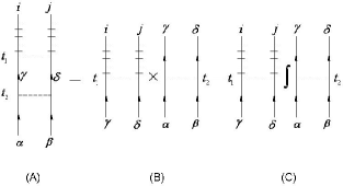
Figure 5: An example of folded-diagram factorization.

The concept of folding can be illustrated by the following factorization operation. The time integral contained in diagram (A) has the limits $0>t_{1}>t_{2}>-\infty$, i.e. $\int^{0}_{-\infty}dt_{1}\int^{t_{1}}_{-\infty}dt_{2}$. For (B), the integrations over $t_{1}$ and $t_{2}$ are independent, both from $-\infty$ to 0. Clearly (A) is not equal to (B). The folded diagram in this case is defined as the “error” introduced by the factorization of (A) into (B), namely diagram (C) is the folded diagram given by

$$(A)=(B)-(C).$$ (23)

In fact they have the values

$$(A)=|\Phi_{ij}\rangle\frac{V_{ij,\gamma\delta}V_{\gamma\delta,\alpha\beta}}{(\epsilon_{\alpha}+\epsilon_{\beta}-\epsilon_{i}-\epsilon_{j})(\epsilon_{\alpha}+\epsilon_{\beta}-\epsilon_{\gamma}-\epsilon_{\delta})},$$ (24)

$$(B)=|\Phi_{ij}\rangle\frac{V_{ij,\gamma\delta}V_{\gamma\delta,\alpha\beta}}{(\epsilon_{\gamma}+\epsilon_{\delta}-\epsilon_{i}-\epsilon_{j})(\epsilon_{\alpha}+\epsilon_{\beta}-\epsilon_{\gamma}-\epsilon_{\delta})},$$ (25)

$$(C)=|\Phi_{ij}\rangle\frac{V_{ij,\gamma\delta}V_{\gamma\delta,\alpha\beta}}{(\epsilon_{\gamma}+\epsilon_{\delta}-\epsilon_{i}-\epsilon_{j})(\epsilon_{\alpha}+\epsilon_{\beta}-\epsilon_{i}-\epsilon_{j})}.$$ (26)

When we have a degenerate model space, then $(\epsilon_{\alpha}+\epsilon_{\beta})=(\epsilon_{\gamma}+\epsilon_{\delta})$ and (A) and (B) both become divergent. It is of interest that the folded diagram (C) is still well defined in this case; (C) is a finite quantity extracted from two divergent ones.

Using the above folded-diagram factorization, one can obtain an energy-independent effective interaction given by [12, 13]

$$V_{eff} = \hat{Q}-\hat{Q}^{{}^{\prime}}\int\hat{Q}+\hat{Q}^{{}^{\prime}}\int\hat{Q}\int\hat{Q}$$ (27)

$$-\hat{Q}^{{}^{\prime}}\int\hat{Q}\int\hat{Q}\int\hat{Q}\cdots.$$

This is a well-known folded-diagram expansion for the model-space effective interaction [12, 13], which is energy-independent and valence-linked. For the case of a one-dimensional model space, the above expansion reduces to the well-known Goldstone linked-diagram expansion [12, 14]. The folded-diagram expansion is basically an extension of the Goldstone expansion to a multi-dimensional model space.

Let us now explain the various terms of Eq. (21). Each integral sign in the above denotes a “fold” [13]. For instance the last term in the equation is a three-fold term; it has three integral signs. $\hat{Q}$ represents a so-called $\hat{Q}$-box, which may be schematically written as

$$\hat{Q}(\omega)=[PVP+PVQ\frac{1}{\omega-QHQ}QVP]_{linked}.$$ (28)

(For convenience, we shall use $V$ in place of $V_{NN}$.) In fact the $\hat{Q}$-box is an irreducible vertex function where the intermediate states between any two vertices must belong to the $Q$ space. (Note that we use $Q$, without hat, to denote the $Q$-space projection operator.) It contains valence-linked diagrams only, as indicated by the subscript “linked”. The $\hat{Q}^{\prime}$-box of Eq. (21) is defined as ($\hat{Q}-PVP$). In Fig. 4 some low-order $\hat{Q}$-box diagrams for nuclei with two valence nucleons, such as ${}^{18}O$, are shown. Note that the intermediate state between two successive vertices must be in the $Q$-space. For example, in an sd-shell calculation of ${}^{18}O$ the intermediate state of diagram d5 of Fig. 4 must have at least one particle outside the sd-shell.

For a nucleus of $n$ valence nucleons, such as $n=3$ for ${}^{19}O$, the above $V_{eff}$ contains one-body (1b), two-body (2b),…and up to $n$-body ($n$b) terms [12], namely

$$V_{eff} = V_{eff}(1b)+V_{eff}(2b)+V_{eff}(3b)+\cdots$$ (29)

$$+V_{eff}(nb).$$

An important feature of this $V_{eff}$ is its “nucleus independence”. As an example, the $V_{eff}(2b)$ for nuclei ${}^{A}O$, $A=18,19,20,...$ are all the same according to the above folded-diagram method. This is a desirable feature, as it allows us to use the same two-body effective interaction derived for $A=18$ for all the other sd-shell nuclei. However the many-body forces for different nuclei are different. For example ${}^{19}O$ and ${}^{20}O$ have the same $V_{eff}(3b)$, but ${}^{20}O$ has in addition $V_{eff}(4b)$ while ${}^{19}O$ does not.

The above $V_{eff}$ allows us to use the experimental sp energies. To illustrate, let us consider the 0d1s-shell nuclei. The energies of ${}^{17}O$ is given by $(H_{0}+V_{eff}(1b))$ which corresponds to the experimental sp energies of ${}^{17}O$. Since $V_{eff}(1b)$ is the same for all the 0d1s-shell nuclei, we can use these sp energies for all of them. Thus the model-space secular equation is of the form shown in Eq. (10). Note, however, when experimental sp energies are employed, the effective interaction is at least two-body, namely $H_{eff}=H_{0}^{expt}+V_{eff}(nb);n\geq 2$. As indicated in Eq. (10), the energies given by $H_{eff}$ are $E_{m}-E_{0}^{core}$. This subtraction is because the diagrams contained in the folded-diagram expansion are all valenced-linked, unlinked core-excitation diagrams having been removed [12, 13].

We now come to the calculation of the folded-diagram expansion for the effective interaction. The expansion of Eq. (21) may be rewritten as

$$V_{eff}=F_{0}+F_{1}+F_{2}+F_{3}+F_{4}+\cdots,$$ (30)

where $F_{n}$ denotes all the diagrams with $n$ folds. If the model space is degenerate, i.e. $PH_{0}P=W_{0}$ is constant, then the various $F$ terms can be conveniently written as

$$F_{0} = \hat{Q}$$

$$F_{1} = \hat{Q_{1}}\hat{Q}$$

$$F_{2} = \hat{Q_{2}}\hat{Q}\hat{Q}+\hat{Q_{1}}\hat{Q}$$

$$F_{3} = \hat{Q_{3}}\hat{Q}\hat{Q}\hat{Q}+\hat{Q_{2}}\hat{Q_{1}}\hat{Q}\hat{Q}+\hat{Q_{2}}\hat{Q}\hat{Q_{1}}\hat{Q}$$

$$+\hat{Q_{1}}\hat{Q_{2}}\hat{Q}\hat{Q}+\hat{Q_{1}}\hat{Q_{1}}\hat{Q_{1}}\hat{Q}$$

$$\vdots$$ (31)

where the $\hat{Q}$-box derivatives are

$$\hat{Q}_{n}=\left.\frac{1}{n!}\frac{d^{n}\hat{Q}}{d\omega^{n}}\right|_{\omega=W_{0}}.$$ (32)

In an early calculation for the 0d1s shell [24], the above folded-diagram series was found to converge rather rapidly; the main contribution was from the once-folded term $F_{1}$, $F_{2}$ was much smaller and $F_{3}$ was negligible. However, it would be useful if the series can be summed to all orders.

Two iteration methods for numerically calculating the folded-diagram series to all orders have been developed. One is the Krenciglowa-Kuo (KK) iteration method [25]. This method employs a partial summation framework which has a clear diagrammatic struture, explicitly showing how the folded diagrams are generated and summed in each additional iteration. Another iteration method is the Lee-Suzuki method [26, 27], which has been widely employed in shell-model calculations [4, 5].

Let us outline the Lee-Suzuki method. We define the effective interaction given by the $n$th iteration as $R_{n}$, and the initial condition is chosen as

$$R_{1}=\hat{Q}(\omega=W_{0}),$$ (33)

where $\hat{Q}$ is the irreducible vertex function of Eq. (22). We consider a degenerate model space with $PH_{0}P=W_{0}$. The effective interaction for the second iteration is

$$R_{2}=\frac{1}{1-\frac{d\hat{Q}}{d\omega}\mid_{\omega=W_{0}}}\times\left[H_{0}-W_{0}+\hat{Q}(W_{0})\right],$$ (34)

and for the $n$th iteration we have

$$R_{n} = \frac{1}{1-\hat{Q}_{1}-\sum_{m=2}^{n-1}\hat{Q}_{m}\prod_{k=n-m+1}^{n-1}R_{k}}$$ (35)

$$\times\left[H_{0}-W_{0}+\hat{Q}(W_{0})\right],$$

where $\hat{Q}_{m}$ is the energy derivative of the $\hat{Q}$-box as given by Eq. (26). The Lee-Suzuki method is convenient for calculations, and it usually converges after 3 or 4 iterations.

A difference between the Krenciglowa-Kuo and Lee-Suzuki iteration methods may be pointed out. Recall that for a model space of dimension $d$, $PH_{eff}P$ reproduces only $d$ eigenstates of the full-space $H$. The question is then which $d$ states of $H$ are reproduced by $H_{eff}$. It is of interest that the Lee-Suzuki method reproduces the $d$ lowest (in energy) states of $H$ [26, 27] while the states reproduced by the Krenciglowa-Kuo method are those with the largest $P$-space overlaps [25].

The above methods were originally both formulated for the case of a degenerate $P$-space, namely $PH_{0}P$ is degenerate. Iteration methods for calculating the effective interaction with non-degenerate $PH_{0}P$ have also been developed [28, 29, 30, 31]. The method described in [29] is a simple iteration method, which is outlined below. We denote the effective interaction for the ith iteration as $V_{eff}^{(i)}$ with the corresponding eigenvalues $E$ and eigenfunctions $\chi$ given by

$$[PH_{0}P+V_{eff}^{(i)}]\chi_{m}^{(i)}=E_{m}^{(i)}\chi_{m}^{(i)}.$$ (36)

Here $\chi_{m}$ is the $P$-space projection of the full-space eigenfunction $\Psi_{m}$, namely $\chi_{m}=P\Psi_{m}$. The effective interaction for the next iteration is then

$$V_{eff}^{(i+1)} = \sum_{m}[PH_{0}P+\hat{Q}(E_{m}^{(i)})]|\chi_{m}^{(i)}\rangle\langle\tilde{\chi}_{m}^{(i)}|$$ (37)

$$-PH_{0}P,$$

where the bi-orthogonal states are defined by

$$\langle\tilde{\chi}_{m}|\chi_{m^{\prime}}\rangle=\delta_{m,m^{\prime}}.$$ (38)

Note that in the above $PH_{0}P$ is non-degenerate. The converged eigenvalue $E_{m}$ and eigenfunction $\chi_{m}$ satisfy the $P$-space self-consistent condition

$$(E_{m}(\omega)-H_{0})\chi_{m}=\hat{Q}(\omega)\chi_{m};\,\,\omega=E_{m}(\omega).$$ (39)

To start the iteration, we may use

$$V_{eff}^{(1)}=\hat{Q}(\omega_{0}),$$ (40)

where $\omega_{0}$ is a starting energy chosen to be close to $PH_{0}P$. The converged effective interaction is given by $V_{eff}=V_{eff}^{(n+1)}=V_{eff}^{(n)}$. When convergent, the resultant $V_{eff}$ is independent of $\omega_{0}$, as it is the states with maximum $P$-space overlaps which are selected by this method [25, 29].

For exotic nuclei, we may need to employ a model space consisting of two major shells. An example is the oxygen isotopes with large neutron excess. In this case we may need to use a two-major-shell model space consisting of the $0d1s0f1p$ shells. There is a subtle singularity difficulty associated with such multi-shell effective interactions.

Figure 6: Low-lying states of ${}^{134}Sn$ calculated with the folded-diagram $V_{eff}$ using the $V_{lowk}$ intraction. See section III for further explanations.

Consider the core-polarization diagram d7 of Fig. 4. Let us label its initial state by $(a,b)$, final state by $(c,d)$ and intermediate state by $(c,p,h,b)$. Here $p$ and $h$ denote respectively the particle and hole lines of the diagram. The energy denominator for this diagram is $\Delta=(\epsilon_{a}-\epsilon_{c})-(\epsilon_{p}-\epsilon_{h})$, $\epsilon$ being the single-particle energy. This $\Delta$ may be equal to zero, causing the $\hat{Q}$-box to be singular. For example this happens for $(a,b)=(0f,0f),~{}(c,d)=(0d,0d),~{}p=0d,~{}h=0p$ when a harmonic oscillator $H_{0}$ is used. This singularity is not convenient for the calculation of $V_{eff}$. It is remarkable and interesting that these potential divergences can be circumvented by the recently proposed $Z$-box method [31, 32, 33]. In this method, a vertex function $\hat{Z}$-box is employed. It is related to the $\hat{Q}$-box by

$$\hat{Z}(\omega)=\frac{1}{1-\hat{Q}_{1}(\omega)}[\hat{Q}(\omega)-\hat{Q}_{1}(\omega)P(\omega-H_{0})P],$$ (41)

where $\hat{Q}_{1}$ is the first-order derivative of the $\hat{Q}$-box. The $\hat{Z}$-box considered by Okamoto et al. [32] is for degenerate model spaces ($PH_{0}P=W_{0}$), while we consider here a more general case with non-degenerate $PH_{0}P$. An important property of the above $\hat{Z}$-box is that it is finite when the $\hat{Q}$-box is singular (has poles). Note that $\hat{Z}(\omega)$ satisfies

$$\hat{Z}(\omega)\chi_{m}=\hat{Q}(\omega)\chi_{m}~{}{\rm at}~{}\omega=E_{m}(\omega).$$ (42)

Thus the converged $V_{eff}$ given by the $\hat{Z}$-box is the same as by the $\hat{Q}$-box. In principle, we may use either for its calculation. But the $\hat{Z}$-box is more convenient for the calculation, especially for the multi-shell non-degenerate case where the $\hat{Z}$-box is a well-behaved function while the $\hat{Q}$-box may have singularities [31].

Figure 7: Same as Fig. 6 but for ${}^{132}Te$.

Let us now give a partial summary of what we have done. The formulations presented so far may seem complicated. But the main point is fairly simple. Namely we have shown that a general many-body problem specified by Hamiltonian $H$ can be formally reduced to a model-space problem consisting of a small number of quasi-particles confined in a small model space with effective Hamiltonian $PH_{eff}P$. This Hamiltonian is given by ($H_{0}$ + $V_{eff}$) where $V_{eff}$ is the quasi-particle effective interaction which can be calculated from the above folded-diagram series. Iterative methods for summing up this series for both degenerate and non-degenerate model spaces have been formulated, as described earlier. This $V_{eff}$ method has been successfully applied to shell-model nuclear structure calculations [4, 5].

Figure 8: Same as Fig.6 but for ${}^{136}Te$.

In the following section we shall discuss the low-momentum NN interaction $V_{low-k}$ [34, 35, 36, 37, 38, 39, 40, 41, 42, 43] which will be employed in evaluating the above folded-diagram $V_{eff}$ for shell-model calculations. This approach has indeed been rather successful. As a preview, we display some sample results [5] in Figs. 6-8.

3 Low-momentum NN interaction

In microscopic nuclear structure calculations starting from a fundamental nucleon-nucleon (NN) potential $V_{NN}$, a well-known ambiguity has been the choice of the NN potential. There are a number of successful models for $V_{NN}$, such as the CD-Bonn [8], Argonne V18 [9], Nijmegen [10] and Idaho [11] potentials. A common feature of these potentials is that they all reproduce the empirical deuteron properties and low-energy phase shifts very accurately. But, as illustrated in Figs. 1-2 which show the momentum-space matrix elements, these potentials are in fact quite different from each other. This has been a situation of much concern: certainly we would like to have a “unique” NN potential. If there does exist one unique NN potential, then one is confronted with the difficult question in deciding which, if any, of the existing potential models is the correct one. In the past several years, there have been extensive studies of the so-called low-momentum NN potential $V_{low-k}$ [34, 35, 36, 37, 38, 39, 40, 41, 42, 43]. In the following, we shall discuss this development in some detail.

The potential $V_{low-k}$ is based on the renormalization group (RG) and effective field theory (EFT) approaches [44, 45, 46, 47, 48, 49]. A central theme of the RG-EFT approaches is that in probing physics in the infrared region, it is generally adequate to employ a low-energy (or low-momentum) effective theory. One starts with a chosen underlying theory, in the present case one of the high-precision nucleon-nucleon potential models. There are states of both high and low energy in the theory. Then by a decimation procedure where the high-energy modes are integrated out, one obtains an effective field theory for the low-energy modes. How to carry out this integration is of course an important step. Here the methods of the renormalization group come in. For low-energy physics, one usually employs a model space below a cut-off momentum $\Lambda$, which is typically several hundred MeV. All fields with momentum greater than $\Lambda$ are integrated (or decimated) out, and in this way we obtain an EFT for momentum within $\Lambda$.

It is tempting to apply the above RG-EFT idea to realistic NN potentials. These models all have a built-in strong short-range repulsion, as is well known. As a result, they all have strong high-momentum components. We are quite certain about the physics of the long-range (or low-momentum) part of $V_{NN}$. After all, at the largest distances the nucleon-nucleon potential is essentially just one-pion exchange. However, we are less certain about the very short-range (or high-momentum) part; in most models it is put in by hand phenomenologically. Thus the high-momentum modes of $V_{NN}$ are model dependent. In line with the above RG-EFT approach, it seems to be both of interest and desirable to just “integrate out” the short-range or the high-momentum part of the NN potential, thereby obtaining a low-momentum effective potential $V_{low-k}$. In so doing we are indeed trying to weed out the most uncertain parts of the NN potential. In the following, let us first describe our method for carrying out the above integration. The $V_{low-k}$ derived from different NN potentials will be compared. We shall show that for a specific cut-off momentum $\Lambda$ the $V_{low-k}$ derived from different NN potential models are nearly identical to each other. In addition, it is a smooth potential and appears to be suitable for directly computing shell-model effective interactions.

III.A. $T$-matrix equivalence approach

We now discuss how to calculate $V_{low-k}$. In integrating out the high-momentum parts mentioned earlier, an important requirement is that certain low-energy physics of $V_{NN}$ is exactly preserved by $V_{low-k}$. For the two-nucleon problem, there is one bound state, namely the deuteron. Thus one must require the deuteron properties given by $V_{NN}$ to be preserved by $V_{low-k}$. In nuclear effective-interaction theory, there are several well developed model-space reduction methods. One of them is the Kuo-Lee-Ratcliff (KLR) folded-diagram method [12, 13], which was originally formulated for discrete (bound state) problems. We have discussed this method in detail earlier in section II.

For the two-nucleon problem, we want the effective interaction $V_{low-k}$ to preserve also the low-energy scattering phase shifts, in addition to the deuteron binding energy. Thus we need an effective interaction for scattering (unbound) problems. A convenient framework for this purpose is a $T$-matrix equivalence approach as described below.

We use a continuum model space specified by $k\leq\Lambda$, namely

$$P=\int_{0}^{\Lambda}d\vec{k}\;|\vec{k}\rangle\langle\vec{k}|,$$ (43)

where $k$ is the two-nucleon relative momentum and $\Lambda$ is the cut-off momentum which is also known as the decimation momentum. Its typical value is about 2 $fm^{-1}$ as we shall discuss later. Our purpose is to look for an effective interaction $PV_{eff}P$, with $P$ defined above, which preserves certain properties of the full-space interaction $V_{NN}$ for both bound and unbound states. This effective interaction will be referred to as $V_{low-k}$.

We start from the full-space half-on-shell $T$-matrix

$$T(k^{\prime},k,\omega)=V_{NN}(k^{\prime},k)$$ (44)

$$+{\cal P}\int_{0}^{\infty}q^{2}dqV_{NN}(k^{\prime},q)\frac{1}{\omega-H_{0}(q)}T(q,k,\omega),$$

where $\omega=\varepsilon_{k}$. This is the $T$-matrix for the two-nucleon problem with Hamiltonian $H=H_{0}+V_{NN}$ and $H_{0}$ represents the relative kinetic energy with its eigenvalue denoted by $\varepsilon_{k}$. The symbol ${\cal P}$ denotes the principle value integration.

We then define a $P$-space low-momentum $T$-matrix by

$$T_{low-k}(p^{\prime},p,\omega)=V_{low-k}(p^{\prime},p)$$ (45)

$$+{\cal P}\int_{0}^{\Lambda}q^{2}dqV_{low-k}(p^{\prime},q)\frac{1}{\omega-H_{0}(q)}T_{low-k}(q,p,\omega),$$

where $\omega=\varepsilon_{p}$, $(p^{\prime},p)\leq\Lambda$, and the integration is from 0 to $\Lambda$. We require the equivalence condition

$$T(p^{\prime},p,\varepsilon_{p})=T_{low-k}(p^{\prime},p,\varepsilon_{p});~{}p^{\prime},p\leq\Lambda.$$ (46)

The above equations define the effective low-momentum interaction; it is required to preserve the low-momentum ($\leq\Lambda$) half-on-shell $T$-matrix. Since phase shifts are given by the fully-on-shell $T$-matrix $T(p,p,\varepsilon_{p})$, low-energy phase shifts given by the above $V_{low-k}$ are clearly the same as those of $V_{NN}$.

In the following, let us show that a solution of the above equations may be found by way of a folded-diagram method [34, 13, 12]. The $T$-matrix of Eq. (37) can be written as

$$\langle k^{\prime}|(V+V\frac{1}{e(\varepsilon_{k})}V+V\frac{1}{e(\varepsilon_{k})}V\frac{1}{e(\varepsilon_{k})}V+\cdots)|k\rangle,$$

where $e(\omega)\equiv(\omega-H_{o})$. (For simplicity, we have used $V$ to denote $V_{NN}$.) Note that the intermediate states (represented by 1 in the numerator) cover the entire space. In other words, we have $1=P+Q$ where $P$ denotes the model space (momentum $\leq\Lambda$) and $Q$ its complement. Expanding it out in terms of $P$ and $Q$ and defining a $\hat{Q}$-box as

$$\langle k^{\prime}|\hat{Q}(\omega)|k\rangle$$ (47)

$$=\langle k^{\prime}|[V+V\frac{Q}{e(\omega)}V+V\frac{Q}{e(\omega)}V\frac{Q}{e(\omega)}V+\cdot\cdot\cdot]|k\rangle,$$

one readily sees that the $P$-space portion of the $T$-matrix can be regrouped as a $\hat{Q}$-box series, namely

$$\langle p^{\prime}|T(\omega)|p\rangle=\langle p^{\prime}|[\hat{Q}(\omega)+\hat{Q}(\omega)\frac{P}{e(\omega)}\hat{Q}(\omega)$$ (48)

$$+\hat{Q}(\omega)\frac{P}{e(\omega)}\hat{Q}(\omega)\frac{P}{e(\omega)}\hat{Q}(\omega)+\cdot\cdot\cdot]|p\rangle,$$

where $\omega=\varepsilon_{p}$. Note that the intermediate states of each $\hat{Q}$-box all belong to the Q-space. Denoting each $\hat{Q}$ by a circle, the above $T$-matrix is given by the sum of all the terms in the left column of Fig. 9 (namely $T=A+B+C+\cdots$).

Figure 9: Expansion of $T$-matrix in terms of $\hat{Q}$-box (represented by a circle). Each integral sign represents a fold

All the $\hat{Q}$-boxes in the above equation have the same energy variable, namely $\varepsilon_{p}$. Let us introduce a folded-diagram factorization [12]: We factorize the two-$\hat{Q}$-box term as

$$\langle p^{\prime}|\hat{Q}(\varepsilon_{p})\frac{P}{e(\varepsilon_{p})}\hat{Q}(\varepsilon_{p})|p\rangle=$$ (49)

$$\sum_{p^{\prime\prime}}\langle p^{\prime}|\hat{Q}(\varepsilon_{p}^{\prime\prime})|p^{\prime\prime}\rangle\langle p^{\prime\prime}|\frac{P}{e(\varepsilon_{p})}\hat{Q}(\varepsilon_{p})|p\rangle-\langle p^{\prime}|\hat{Q}^{\prime}\int\hat{Q}|p\rangle,$$

where the last term is the once-folded two-$\hat{Q}$-box term. The folded term is simply the difference between the original and factorized two-$\hat{Q}$-box terms. Schematically the above factorization is written as

$$\hat{Q}\frac{P}{e}\hat{Q}=\hat{Q}\times\hat{Q}-\hat{Q}^{\prime}\int\hat{Q}.$$ (50)

Diagrammatically, this equation is represented by the second equation of Fig. 9, where (B) represents the lhs two-$\hat{Q}$-box term, (B1) the factorized two-$\hat{Q}$-box term and (B2) the corresponding folded term. A subtle difference between the vertex functions $\hat{Q}$ and $\hat{Q}^{\prime}$ may be pointed out. $\hat{Q}$ has diagrams with one, two, three,… $V$ vertices. Those with one $V$ vertex are energy independent, and for them there is no folded-diagram correction. Thus $\hat{Q}^{\prime}$ is the same as $\hat{Q}$ except with its diagrams first order in $V$ removed. This relation remains the same for higher order folded diagrams.

Similarly we can factorize the three-$\hat{Q}$-box term as

$$\hat{Q}\frac{P}{e}\hat{Q}\frac{P}{e}\hat{Q} = \hat{Q}\times\hat{Q}\frac{P}{e}\hat{Q}-[\hat{Q}^{\prime}\int\hat{Q}]\times\hat{Q}$$ (51)

$$+\hat{Q}^{\prime}\int\hat{Q}\int\hat{Q},$$

where the last term is a twice-folded three-$\hat{Q}$-box term. Diagrammatically this equation is represented by the third equation of Fig. 9, where (C) denotes the lhs three-$\hat{Q}$-box term while the corresponding factorized, factorized and once-folded, and twice-folded terms are represented respectively by diagrams (C1), (C2) and (C3).

The folded-diagram factorization for the four-$\hat{Q}$-box term of $T$ can be carried out in a similar way. And this four $\hat{Q}$-box term of $T$ is factorized into four terms (D1) to (D4). (These terms are not shown in Fig. 9, but their structure is closely similar to the three-$\hat{Q}$-box factorization. For example, (D4) is of the form -$\hat{Q}\int\hat{Q}\int\hat{Q}\int\hat{Q}$.) Continuing this procedure, a simple structure becomes transparent. The sum of the diagrams (A), (B2), (C3), (D4),… of Fig. 9 is just the effective interaction

$$V_{low-k} = \hat{Q}-\hat{Q^{\prime}}\int\hat{Q}+\hat{Q^{\prime}}\int\hat{Q}\int\hat{Q}$$ (52)

$$-\hat{Q^{\prime}}\int\hat{Q}\int\hat{Q}\int\hat{Q}+\cdots$$

The sum of the diagrams (B1), (C2), (D3), … is just $V_{low-k}\frac{1}{e}\hat{Q}$. Since $T$ is the sum of the diagrams (A), (B), (C), (D), … it is readily seen that by regrouping the diagrams of Fig. 9 we have the $T$-matrix equation $T=V_{low-k}+V_{low-k}\frac{1}{e}T$. Namely the $V_{low-k}$ given by the above equation is a solution of Eqs. (30-32).

Note that this is just the KLR folded-diagram effective interaction [12, 13] as given earlier in Eq. (21). The KLR method was originally formulated for bound-state problems. We now see that it is also applicable to scattering problems; it preserves the half-on-shell $T$-matrix. This implies the preservation of not only the low-energy phase shifts (which are given by the fully-on-shell $T$-matrix) but also the low-momentum components of the scattering wave functions.

We have shown above that certain low-energy physical quantities given by the full-momentum potential $V_{NN}$ are preserved by the low-momentum potential $V_{low-k}$. This preservation is an important point, and it should be numerically checked, to see for instance if the deuteron binding energy and low-energy phase shifts given by $V_{NN}$ are indeed reproduced by $V_{low-k}$. We have checked the deuteron binding energy $BE_{d}$ given by $V_{low-k}$. For a range of $\Lambda$, such as $0.5fm^{-1}\leq\Lambda\leq 3fm^{-1}$, $BE_{d}$ given by $V_{low-k}$ agrees very accurately (to 4 places after the decimal point) with that given by $V_{NN}$. We have also checked the phase shifts and the $T$-matrix $T(p^{\prime},p,\omega=p^{2})$ with $(p^{\prime},p)\leq\Lambda$; very good agreement between these quantities given by $V_{NN}$ and $V_{low-k}$ were obtained.

An important question in our approach is the choice of the momentum cut-off $\Lambda$. Phase shifts are given by the fully-on-shell $T$-matrix, $T(p,p,\varepsilon_{p})$. Hence for a chosen $\Lambda$, $V_{low-k}$ can only produce phase shifts up to $E_{lab}=2\hbar^{2}\Lambda^{2}/M$, $M$ being the nucleon mass. Realistic NN potentials are constructed to fit empirical phase shifts up to $E_{lab}\approx 350$ MeV [8]. It is reasonable then to require our $V_{low-k}$ to reproduce phase shifts also up to this energy. Thus one should use $\Lambda$ in the vicinity of 2 $fm^{-1}$.

Figure 10: Comparison of ${}^{1}S_{0}-{{}^{1}S_{0}}$ diagonal momentum-space matrix elements $V_{low-k}(k,k)$ of Paris [6], CD-Bonn [8], Argonne [9], Nijmegen [10] and Idaho [11] potentials.

In Figs. 10-11, we compare some $V_{low-k}(k,k)$ matrix elements calculated from several $V_{NN}$ potentials. A decimation momentum of $\Lambda=2.0fm^{-1}$ is used in the $V_{low-k}$ calculation. It is seen that the matrix elements given by the various potentials are nearly identical, in sharp contrast to Figs. 1-2 where the corresponding $V_{NN}(k,k)$ matrix elements are vastly different. This is an interesting result, suggesting that the $V_{low-k}$ interactions derived for different realistic $V_{NN}$ potentials are nearly uinique [40]. Note that these $V_{NN}$ potentials all reproduce the low-energy two-nucleon experimental data (deuteron binding energy and NN phase shifts up to $E_{lab}\simeq 350$ MeV) very well.

Figure 11: Same as Fig. 10 but for the ${}^{3}S_{1}-{{}^{3}S_{1}}$ channel.

Extensive shell-model calculations based on $V_{low-k}$ have been carried out with rather encouraging results (see e.g., Ref. [5]). To illustrate, we compare in Figs. 7-9 the calculated spectra with the experimental ones for three nuclei ${}^{134}Sn$, ${}^{132}Te$ and ${}^{136}Te$. The $V_{low-k}$ obtained from the CD-Bonn potential [8] using a decimation momentum $\Lambda=2.0fm^{-1}$ has been employed [5]. As seen the calculated spectra agree with the experimental ones rather satisfactorily.

For many years, the Brueckner $G$-matrix interaction was employed in nuclear calculations using realistic NN interactions [4]. Both $G$-matrix and $V_{low-k}$ transform, or tame, the NN interactions with strong repulsive cores into smooth interactions without such cores, the latter being much simpler for calculations than the former. A difference between these two interactions may be mentioned. The $G$-matrix interaction is energy dependent while the $V_{low-k}$ is not. This makes the latter more convenient in applications [5, 50, 51, 52].

III.B. Counter terms

A main point of the RG-EFT theory is that low-energy physics is not sensitive to fields beyond a cut-off scale $\Lambda$. Thus for treating low-energy physics, one just integrates out the fields beyond a cut-off scale $\Lambda$, thereby obtaining a low-energy effective field theory. In RG-EFT, this integrating out, or decimation, generates an infinite series of counter terms [47] which are simple power series in momentum. This is a very useful and interesting result. When we derive our low-momentum interaction, the high-momentum modes of the input interaction are integrated out. Does this decimation also generate a series of counter terms? If so, what are the counter terms so generated? Holt, Kuo, Brown and Bogner [42] have studied this question, and we would like to review their results here.

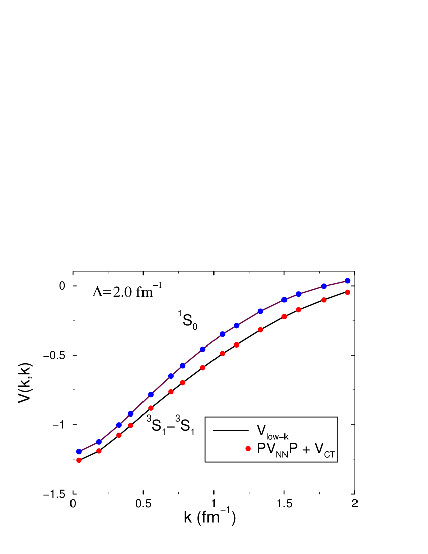
Figure 12: Comparison of $V_{low-k}$ with $PV_{NN}P$ plus counter terms for ${}^{1}S_{0}$ and ${}^{3}S_{1}$ channels.

Similar to the usual counter term approach, we assume that the difference between $V_{low-k}$ and $V_{NN}$ can be accounted for by a series of counter terms. Specifically, we consider

$$V_{low-k}(q,q^{\prime}) \simeq V_{NN}(q,q^{\prime})$$ (53)

$$+V_{counter}(q,q^{\prime});~{}(q,q^{\prime})\leq\Lambda,$$

where $V_{NN}$ is the free-space NN potential from which $V_{low-k}$ is derived and the counter term potential is given as a power series

$$V_{counter}(q,q^{\prime})=$$

$$C_{0}+C_{2}q^{2}+C_{2}^{\prime}q^{\prime 2}+C_{4}(q^{4}+q^{\prime 4})+C_{4}^{\prime}q^{2}q^{\prime 2}$$

$$+C_{6}(q^{6}+q^{\prime 6})+C_{6}^{\prime}q^{4}q^{\prime 2}+C^{\prime\prime}_{6}q^{2}q^{\prime 4}+....$$ (54)

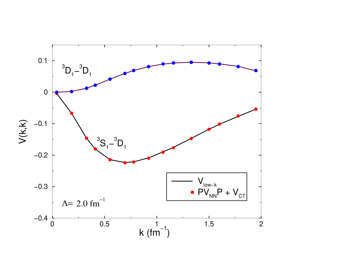
Figure 13: Same as Fig. 12 but for ${}^{3}D_{1}$ and ${}^{3}S_{1}-^{3}D_{1}$ channels.

The counter term coefficients are determined using standard fitting techniques so that the right hand side of Eq. (48) provides a best fit to the left hand side of the same equation. We perform this fitting over all partial wave channels, and find consistently good agreement. In Fig. 12 we compare some ${}^{1}S_{0}$ and ${}^{3}S_{1}$ matrix elements of $(PV_{NN}P+V_{CT})$ with those of $V_{low-k}$ for momenta below the cutoff $\Lambda$. Here $P$ denotes the projection operator for states with momentum less than $\Lambda$. A similar comparison for ${}^{3}D_{1}$ and ${}^{3}S_{1}-{{}^{3}D_{1}}$ channels is displayed in Fig. 13. The agreement is indeed very good, and also for phase shifts as illustrated in Fig. 14.

Now let us examine the counter terms themselves. In Table 2, we list some of the counter term coefficients, using CD-Bonn as our bare potential. In the table we list only the counter terms for the ${}^{1}S_{0}$ and ${}^{3}S_{1}-{{}^{3}D_{1}}$ partial waves; we have found that the counter terms for all the other waves are much smaller. This tells us an interesting result, namely, except for the above two channels, $V_{low-k}$ is very similar to $V_{NN}$ alone. We also point out that the coefficients $C_{6}$ are found to be very small, indicating that the above power series expansion converges rapidly. In the last row of the table, we list the rms deviations between $V_{low-k}$ and $PV_{NN}P+V_{counter}$; the fit is indeed very good.

As shown in the table, the counter terms are all rather small except for $C_{0}$ and $C_{2}$ of the $S$ waves. This is consistent with the RG-EFT approach where the counter term potential is given as a delta function plus its derivatives [47].

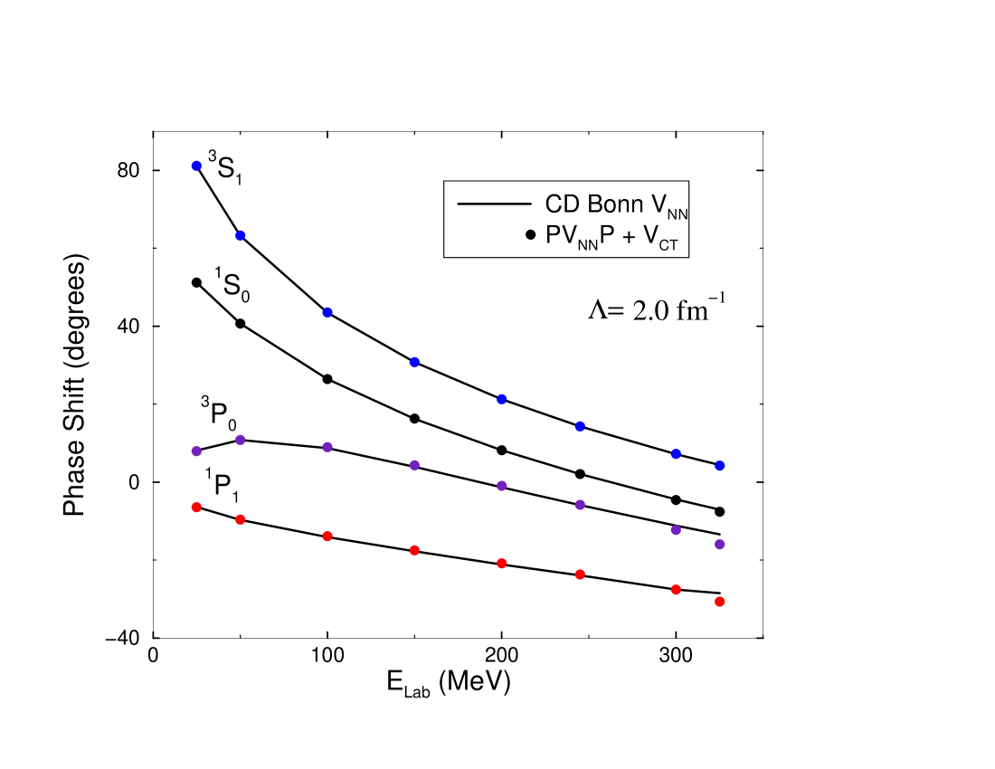
Figure 14: Comparison of phase shifts calculated from $V_{low-k}$ with those from $PV_{NN}P$ plus counter terms.

Comparing counter term coefficients for different $V_{bare}$ potentials can illustrate key differences between those potentials. For example, we have found that the ${}^{1}S_{0}$ $C_{0}$ coefficients for the CD-Bonn [8], Nijmegen [10], Argonne [9] and Paris [6] NN potentials are respectively -0.158, -0.570, -0.753 and -1.162. Similarly, the ${}^{3}S_{1}$ $C_{0}$ coefficients for these potentials are respectively -0.467, -1.082, -1.148 and -2.224. That the $C_{0}$ coefficients for these potentials are significantly different is a reflection that the short-range repulsions built into these potentials are different. For instance, the Paris potential effectively has a very strong short-range repulsion and consequently its $C_{0}$ is much larger than the $C_{0}$ of the others. The short-range repulsion contained in $NN$ potentials is uncertain and model dependent. Further study is needed for its understanding.

Table 2: Coefficients of the counter terms for $V_{low-k}$ obtained from the CD-Bonn potential using $\Lambda=2fm^{-1}$. The unit for the combined quantity $C_{n}k^{n}$ is $fm$, with momentum $k$ in units of $fm^{-1}$.

	${}^{1}S_{0}$	${}^{3}S_{1}$	${}^{3}S_{1}-^{3}D_{1}$	${}^{3}D_{1}$
$C_{0}$	-0.1580	-0.4646	0	0
$C_{2}$	-0.0131	0.0581	-0.0017	-0.0005
$C_{2}^{\prime}$	-0.0131	0.0581	0.0301	-0.0005
$C_{4}$	0.0004	-0.0011	-0.0013	0.0006
$C_{4}^{\prime}$	-0.0011	-0.0113	-0.0047	-0.0018
$C_{6}$	-0.0004	-0.0004	0.0006	-0.0001
$C_{6}^{\prime}$	-0.0005	0.0005	-0.0001	-0.0001
$C_{6}^{\prime\prime}$	-0.0005	0.0005	-0.0003	-0.0001
$\Delta_{rms}$	0.0002	0.0003	0.0028	0.0003

As shown in the Table, the $C$ coefficients for the          ${}^{3}S_{1}-{{}^{3}D_{1}}$ channel are all very small. Thus the counter term for the NN tensor force is nearly vanishing and consequently $V_{low-k}(tensor)\simeq V_{NN}(tensor)$. It appears that the tensor force is exempted from renormalization. It should be of interest to further study this possible exemption property of the tensor force.

III.C. Hermitian low-momentum interactions It should be pointed out that the low-momentum NN interaction given by the above folded-diagram expansion is not Hermitian. This is not a desirable feature, and one would like to have an interaction which is Hermitian. Methods for deriving Hermitian effective interactions have been developed by Okubo [53] and Andreozzi [54]. A general framework for constructing Hermitian effective interactions was recently studied by Holt, Kuo and Brown [43]. In this section, we shall discuss their method for derivation of Hermitian effective interactions. As we shall see shortly, one can in fact construct a family of Hermitian low-momentum NN interactions that are phase-shift equivalent.

Let us denote the folded-diagram low-momentum NN interaction as $V_{LS}$. (Recall that we have used the Lee-Suzuki (LS) method for its derivation.) $V_{LS}$ preserves the half-on-shell $T$-matrix $T(k^{\prime},k,k^{2})$ for $(k^{\prime},k)\leq\Lambda$. If we relax this half-on-shell constraint, we can obtain low-momentum NN interactions which are Hermitian. (Note the Hermitian potentials discussed below all preserve the fully on-shell $T$-matrix and are phase-shift equivalent [43].)

The model-space secular equation for $V_{LS}$ is

$$P(H_{0}+V_{LS})P\chi_{m}=E_{m}\chi_{m},$$ (55)

where $\{E_{m}\}$ is a subset of the eigenvalues $\{E_{n}\}$ of the full-space Schroedinger equation $(H_{0}+V)\Psi_{n}=E_{n}\Psi_{n}$. $\chi_{m}$ is the $P$-space projection of the full-space wave function $\Psi_{m}$, namely $\chi_{m}=P\Psi_{m}$. The above effective interaction may be rewritten in terms of a wave operator $\omega$, namely

$$PV_{LS}P=Pe^{-\omega}(H_{0}+V)e^{\omega}P-PH_{0}P,$$ (56)

where $\omega$ possesses the usual properties: $\omega=Q\omega P;\chi_{m}=e^{-\omega}\Psi_{m};\omega\chi_{m}=Q\Psi_{m}.$ Here $Q$ is the complement of $P$, $P+Q=1$.

While the full-space eigenvectors $\Psi_{n}$ are orthogonal to each other, the model-space eigenvectors $\chi_{m}$ are clearly not so and consequently the effective interaction $V_{LS}$ is not Hermitian. We now make a $Z$ transformation such that

$$Z\chi_{m} = v_{m};$$

$$\langle v_{m}\mid v_{m^{\prime}}\rangle = \delta_{mm^{\prime}};~{}m,m^{\prime}=1,d,$$ (57)

where $d$ is the dimension of the model space. This transformation reorients the vectors $\chi_{m}$ such that they become orthonormal to each other. We assume that $\chi_{m}$’s ($m=1,...,d$) are linearly independent so that $Z^{-1}$ exists, otherwise the above transformation is not possible. Since $v_{m}$ and $Z$ exist entirely within the model space, we can write $v_{m}=Pv_{m}$ and $Z=PZP$.

Using Eq. (52), we transform Eq. (50) into

$$Z(H_{0}+V_{LS})Z^{-1}v_{m}=E_{m}v_{m},$$ (58)

which implies

$$Z(H_{0}+V_{LS})Z^{-1}=\sum_{m\epsilon P}E_{m}|v_{m}\rangle\langle v_{m}|.$$ (59)

Since $E_{m}$ is real (it is an eigenvalue of $(H_{0}+V)$ which is Hermitian) and the vectors $v_{m}$ are orthonormal to each other, $Z(H_{0}+V_{LS})Z^{-1}$ is clearly Hermitian. The non-Hermitian secular equation, Eq. (12), is now transformed into a Hermitian model-space eigenvalue problem

$$P(H_{0}+V_{herm})Pv_{m}=E_{m}v_{m}$$ (60)

with the Hermitian effective interaction

$$V_{herm}=Z(H_{0}+V_{LS})Z^{-1}-PH_{0}P,$$ (61)

or equivalently

$$V_{herm}=Ze^{-\omega}(H_{0}+V)e^{\omega}Z^{-1}-PH_{0}P.$$ (62)

To calculate $V_{herm}$, we must first have the $Z$ transformation. Since there are certainly many ways to construct $Z$, this generates a family of Hermitian effective interactions, all originating from $V_{LS}$. For example, we can construct $Z$ using the familiar Schmidt orthogonalization procedure, namely:

$$v_{1} = Z_{11}\chi_{1}$$

$$v_{2} = Z_{21}\chi_{1}+Z_{22}\chi_{2}$$

$$v_{3} = Z_{31}\chi_{1}+Z_{32}\chi_{2}+Z_{33}\chi_{3}$$

$$v_{4} = ......,$$ (63)

with the matrix elements $Z_{ij}$ determined from Eq. (52). We denote the Hermitian effective interaction using this $Z$ transformation as $V_{schm}$. Clearly there is more than one such Schmidt procedure. For instance, we can use $v_{2}$ as the starting point, which gives $v_{2}=Z_{22}\chi_{2}$, $v_{3}=Z_{31}\chi_{1}+Z_{32}\chi_{2}$, and so forth. This freedom in choosing the orthogonalization procedure actually gives us many ways to generate a Hermitian interaction, and this is our family of Hermitian interactions produced from $V_{LS}$.

We now show how some well-known Hermitization transformations relate to (and in fact, are special cases of) ours. We first look at the Okubo transformation [53]. From the properties of the wave operator $\omega$, we have

$$\langle\chi_{m}|(1+\omega^{+}\omega)|\chi_{m^{\prime}}\rangle=\delta_{mm^{\prime}}.$$ (64)

It follows that an analytic choice for the $Z$ transformation is

$$Z=P(1+\omega^{+}\omega)^{1/2}P.$$ (65)

This leads to the Hermitian effective interaction

$$V_{okb-1}=P(1+\omega^{+}\omega)^{1/2}P(H_{0}+V_{LS})P(1+\omega^{+}\omega)^{-1/2}P$$

$$\hskip 22.76228pt-PH_{0}P.$$ (66)

It is easily seen that the above is equal to the Okubo Hermitian effective interaction

$$V_{okb}=P(1+\omega^{+}\omega)^{-1/2}(1+\omega^{+})(H_{0}+V)$$

$$\times(1+\omega)(1+\omega^{+}\omega)^{-1/2}P-PH_{0}P,$$ (67)

giving us an alternative expression, Eq. (62), for the Okubo interaction.

There is another interesting choice for the transformation $Z$. As pointed out by Andreozzi [54], the positive definite operator $P(1+\omega^{+}\omega)P$ can be decomposed into two Cholesky matrices, namely

$$P(1+\omega^{+}\omega)P=PLL^{T}P,$$ (68)

where $L$ is a lower triangle Cholesky matrix, $L^{T}$ being its transpose. Since $L$ is real and it is within the $P$-space, we have

$$Z=L^{T}$$ (69)

and the corresponding Hermitian effective interaction from Eq. (56) is

$$V_{cho}=PL^{T}P(H_{0}+V_{LS})P(L^{-1})^{T}P-PH_{0}P.$$ (70)

This is the Hermitian effective interaction of Andreozzi [54].

The Hermitian effective interaction of Suzuki and Okamoto [28, 55] is of the form

$$V_{suzu}=Pe^{-G}(H_{0}+V)e^{G}P-PH_{0}P$$ (71)

with $G=tanh^{-1}(\omega-\omega^{\dagger})$ and $G^{\dagger}=-G$. It has been shown that this interaction is the same as the Okubo interaction [55]. In terms of the $Z$ transformation, it is readily seen that the operator $e^{-G}$ is equal to $Ze^{-\omega}$ with $Z$ given by Eq. (52). Thus, these three well-known Hermitian effective interactions indeed belong to our family. The family of Hermitian potentials are all phase-shift equivalent to $V_{LS}$ [43].

Using a solvable matrix model, one finds that the above Hermitian effective interactions $V_{schm},V_{okb}$ and $V_{cho}$ can be quite different [43] from each other and from $V_{LS}$, especially when $V_{LS}$ is largely non-Hermitian. For the $V_{NN}$ case, it is fortunate that the $V_{low-k}$ coresponding to $V_{LS}$ is only slightly non-Hermitian. As a result, the Hermitian low-momentum NN inteactions corresponding to $V_{schm},V_{okb}$ and $V_{cho}$ are all quite similar to each other and to $V_{LS}$. Thus in applications it is the $V_{low-k}$ corresponding to $V_{LS}$ which is commonly used [5, 43].

4 Brown-Rho scaling and three-nucleon force

As indicated by Figs. 6-8, the $V_{low-k}$ interactions derived from free-space $V_{NN}$ have worked well in shell-model calculations involving mainly valence nucleons. But for infinite symmetric nuclear matter, such free-space two-nucleon interactions alone are unable to reproduce simultaneously the empirical saturation energy and density ($E_{0}/A\simeq-16$ MeV and $n_{0}=0.16$ fm^-3) [15, 16, 56, 57]. To illustrate, we display in Fig. 15 results from a recent nuclear matter calculation [57] using a non-pertubative ring-diagram resummation method that will be outlined later. There the lowest curve (C) is obtained with the free-space BonnS potential [58]. As seen this curve descends rapidly with density, showing no sign of reaching a local minimum at the saturation energy and density. In the present section we outline how this over-binding problem may be overcome by using density-dependent effective interactions generated by the Brown-Rho scaling mechanism [57, 59, 60, 61, 62, 63] or the inclusion of three-nucleon potential $V_{3N}$ [56, 64, 65, 70]. (The symbol $V_{NN}$ will be used to denote the two-nucleon potential.)

Figure 15: Comparison of the EoS for symmetric nuclear matter calculated with and without the new-BR scaling. Transition densities of $n_{1/2}=2.0n_{0}$ (solid square) and $1.5n_{0}$ (open square) are employed. See text for more explanations.

Realistic nucleon-nucleon potentials are mediated by the exchange of mesons such as the $\pi$, $\rho$, $\omega$ and $\sigma$ mesons. In constructing these potentials the meson-nucleon coupling constants (and in some cases their masses) are adjusted to fit the ‘free-space’ NN scattering data. Mesons in a nuclear medium, however, can have properties (masses and couplings) that are different from those in free space, as the former are ‘dressed’ or ‘renormalized’ by their interactions with the medium. Thus, the NN potential in a medium of density $n$, usually denoted by $V_{NN}(n)$, should be different from that in free space.

The well-known Brown-Rho (BR) scaling mechanism [59, 60, 61, 62, 63] provides a schematic framework for deriving such density-dependent interactions. A main result is the universal scaling relation for nucleon and meson masses:

$$\frac{m^{*}_{N}}{m_{N}}\simeq\frac{m^{*}_{\sigma}}{m_{\sigma}}\simeq\frac{m^{*}_{\rho}}{m_{\rho}}\simeq\frac{m^{*}_{\omega}}{m_{\omega}}\simeq\Phi_{BR}(n),$$

$$\Phi_{BR}(n)=1-C\frac{n}{n_{0}},$$ (72)

where $m^{*}$ and $m$ denote respectively the in-medium and in-vacuum masses, and the parameter $C$ has the value $0.15-0.20$. This scaling naturally renders $V_{NN}$ a density-dependent interaction $V_{NN}(n)$. As we shall describe later, it is remarkable that the above simple scaling law, derived in the context of chiral symmetry restoration in dense matter, would have important consequences for traditional nuclear structure physics.

We have carried out several studies on the effects of BR scaling on finite nuclei, nuclear matter and neutron stars [15, 16, 22, 71, 72]. Let us just briefly describe a few of them. For convenience in implementing BR scaling, we have employed the BonnA and/or BonnS one-boson-exchange potentials [7, 58] whose parameters for $\rho$, $\omega$ and $\sigma$ mesons are scaled with the density (in our calculations the meson masses and cut-off parameters are equally scaled). Note that $\pi$ is protected by chiral symmetry and is not scaled. That we scale $\rho$ but not $\pi$ has an important consequence for the tensor force, which plays an important role in the famous Gamow-Teller (GT) matrix element for the ${}^{14}C\rightarrow$ ${}^{14}N$ $\beta$-decay [22]. The tensor force from $\pi$- and $\rho$-meson exchange are of opposite signs. A lowering of only $m_{\rho}$, but not $m_{\pi}$, can significantly suppress the net tensor force strength and thus largely diminish the GT matrix element. In addition, the scaling of the $\omega$ meson introduces additional short-distance repulsion into the nucleon-nucleon interaction, which was found to also contribute to the suppression [23]. With BR-scaling we were able to satisfactorily account for the anomalously-long $T_{1/2}\sim 5730$-yr lifetime of this decay [22].

It may be noted that the BR scaling as given in Eq. (65) is a linear scaling, and it may be suitable for low densities near $n_{0}$ only ($\Phi_{BR}(n)$ of Eq. (67) may become negative for large $n$). For high densities, we need a different scaling such as the new-BR scaling [74]. Before describing this scaling, let us first describe briefly a $V_{low-k}$ ring-diagram formalism [15, 16, 72, 74] on which our nuclear-matter calculations with the new-BR scaling are based.

In this ring-diagram formalism [15, 16, 72, 74] the nuclear-matter ground-state energy is given by the all-order sum of the particle-particle hole-hole ($pphh$) ring diagrams as shown in Fig. 3. The ground-state energy of asymmetric nuclear matter is expressed as $E(n,\alpha)=E^{free}(n,\alpha)+\Delta E(n,\alpha)$ where $E^{free}$ denotes the energy for the non-interacting system and $\Delta E$ is the energy shift due to the NN interaction. We include in general three types of ring diagrams, the proton-proton, neutron-neutron and proton-neutron ones. The proton and neutron Fermi momenta are, respectively, $k_{Fp}=(3\pi^{2}n_{p})^{1/3}$ and $k_{Fn}=(3\pi^{2}n_{n})^{1/3}$, where $n_{p}$ and $n_{n}$ denote respectively the proton and neutron density. The isospin asymmetry parameter is $\alpha\equiv(n_{n}-n_{p})/(n_{n}+n_{p})$. With such ring diagrams summed to all orders, we have

$$\Delta E(n,\alpha) = \int_{0}^{1}d\lambda\sum_{m}\sum_{ijkl<\Lambda}Y_{m}(ij,\lambda)Y_{m}^{*}(kl,\lambda)$$ (73)

$$\times\langle ij|V_{\rm low-k}|kl\rangle,$$

where $\lambda$ is a strength parameter, integrated from 0 to 1. The transition amplitudes $Y$ are obtained from a $pphh$ RPA equation [15, 16, 57]. These $Y$ amplitudes represent

$$Y_{m}(\alpha,\beta)=\langle\Psi_{0}|a_{\alpha}^{\dagger}a_{\beta}^{\dagger}|\Psi_{m}\rangle,$$

$$~{}(\alpha,\beta)=(h,h^{\prime})~{}or~{}(p,p^{\prime}),$$ (74)

where $\Psi_{0}$ and $\Psi_{m}$ are respectively the ground state and $m$th excited state of nuclear matter with two additional particles or holes. $Y_{m}(p,p^{\prime})$ is a measure of the particle-particle excitations in the ground state. Setting $Y_{m}(p,p^{\prime})$=0 means the ground state is taken to be the closed Fermi sea, and the above ring-diagram method reduces to the usual HF method where only the first-order ring diagram (diagram (a) of Fig. 3) is included for the energy shift. In this case, the above energy shift becomes $\Delta E(n,\alpha)_{HF}=\frac{1}{2}\sum n_{i}n_{j}\langle ij|V_{\rm low-k}|ij\rangle$ where $n_{k}$=(1,0) if $k(\leq,>)k_{Fp}$ for protons and $n_{k}$=(1,0) if $k(\leq,>)k_{Fn}$ for neutrons.

The above $V_{low-k}$ ring-diagram framework has been applied to symmetric and asymmetric nuclear matter [15, 16] and to the nuclear symmetry energy [72]. This framework has also been tested by applying it to dilute cold neutron matter in the limit that the ${}^{1}S_{0}$ scattering length of the underlying interaction approaches infinity [75, 76]. This limit – which is a conformal fixed point – is usually referred to as the unitary limit. For many-body systems at this limit, the ratio $\xi\equiv E_{0}/E_{0}^{free}$ is expected to be a universal constant of value $\sim 0.44$. ($E_{0}$ and $E_{0}^{free}$ are, respectively, the interacting and non-interacting ground-state energies of the many-body system.) The above ring-diagram method has been used to calculate neutron matter using several very different unitarity potentials (a unitarity CDBonn potential obtained by tuning its meson parameters, and several square-well unitarity potentials) [75, 76]. The $\xi$ ratios given by our calculations for all these different unitarity potentials are all close to 0.44, in good agreement with the Quantum-Monte-Carlo results (see [76] and references quoted therein). In fact our ring-diagram results for $\xi$ are significantly better than those given by HF and BHF (Brueckner HF) [75, 76]. The above unitary calculations have provided satisfactory results, supporting the reliability of our $V_{low-k}$ ring-diagram framework for calculating the nuclear matter EoS.

We now describe the new-BR scaling [74] on which the results shown in Fig. 15 are based. The idea behind this scaling is that when a large number of skyrmions as baryons are put on an FCC (face-centered-cubic) crystal to simulate dense matter, the skyrmion matter undergoes a transition to a matter consisting of half-skyrmions [77] in BCC (body-centered-cubic) configuration at a density that we shall denote as $n_{1/2}$. This density is difficult to pin down precisely but it is more or less independent of the mass of the dilaton scalar, the only low-energy degree of freedom that is not well-known in free space. The density at which this occurs has been estimated to lie typically between 1.3 and 2 times normal nuclear matter density $n_{0}$  [78]. In our model, nuclear matter is separated into two regions I and II respectively for densities $n\leq n_{1/2}$ and $n>n_{1/2}$. As inferred by our model, they have different scaling functions

$$\Phi_{i}(n)=\frac{1}{1+C_{i}\frac{n}{n_{0}}},~{}~{}i=I,II.$$ (75)

It has been found that both the BR and new-BR scalings are important for nuclear-matter saturation [15, 16, 71, 74]. The EoS shown by (A) and (B) of Fig. 15 are obtained with the new-BR scaling with $n_{1/2}=1.5n_{0}$ and 2.0$n_{0}$ respectively. Both give an energy per nucleon $E_{0}/A=-15$ MeV, saturation density $k_{F}=1.30fm^{-1}$ and compression modulus $K$=208 MeV, all in satisfactory agreement with the empirical values [74]. We believe that this scaling works well for low densities of $n<\sim 1.5n_{0}$.

As described in [74], we employ in our new-BR scaling calculations the BonnS potential [58] with scaling parameters $C_{\rho}$=0.13, $C_{\sigma}$=0.121, $C_{\omega}$=0.139 , $C_{N}$=0.13 and $C_{g,\rho}=C_{g,\omega}$=0 for region I, where $C_{g}$ is the associated scaling of the meson-nucleon coupling constant. For region II the scaling parameters are $C_{\rho}$=0.13, $C_{\sigma}$=0.121, $C_{\omega}$=0.139 , $C_{g,\rho}$=0.13, $C_{g,\omega}$=0 and $m^{*}_{N}/m_{N}=y(n)$=0.77 for (A) and 0.78 for (B). Note that this scaling has some special features: In region I the coupling constants $g_{\rho N}$ and $g_{\omega N}$ are not scaled, while in region II only the coupling constant $g_{\rho N}$ is scaled. Also in region II the nucleon mass is a density-independent constant as given earlier. Note that our choices for the $C$ parameters are consistent with the Ericson scaling which is based on a scaling relation for the quark condensate $\frac{<\bar{q}q>^{*}}{<\bar{q}q>}$ [79]. According to this scaling, at low densities one should have $C\simeq D/3$ with $D=0.35\pm 0.06$.

Figure 16: Comparison of our calculated $p(n)$ for neutron matter (upper panel) and symmetric nuclear matter (lower panel) with the empirical constraints of Danielewicz et al. [80]. For neutron matter, the stiff and soft constraints are denoted respectively by the upper and lower box.

¿From heavy-ion collision experiments, Danielewicz et al. [80] have obtained constraints for the pressure-density EoS $p(n)$ of nuclear matter up to densities $\sim 4.5n_{0}$. To test this new-BR scaling in the high-density region, the pressure EoS $p(n)$ up to the above densities has been calculated. [74] The results are presented in Fig. 16 where the calculated $p(n)$ for neutron matter (upper panel) and symmetric nuclear matter (lower panel) are compared with the Danielewicz constraints [80]. For neutron matter, there are two constraints, one for stiff EoS (upper box) and the other for soft EoS (lower box). The EoSs calculated with parameters A and B are denoted by solid- and open-square respectively. As seen, the results are in satisfactory agreements with the empirical constraints of [80].

Also based on such experiments, there has been much progress in determining the nuclear symmetry energy $E_{sym}$ up to densities as high as $\sim 5n_{0}$ [81, 82, 83]. Thus an application of the new-BR scaling to the calculation of $E_{sym}$ would provide an important test for this scaling in the region with $n>n_{1/2}$. As displayed in Fig. 17, the symmetry energies calculated from the new-BR EoS [74] are in good agreement with the experimental constraints of Li et al. [81, 82] and Tsang et al. [83]. As seen, there are two constraints from Li, one for stiff EoS and the other for soft EoS. The calculated results are close to the stiff constraint at high denities, but slightly lower than both at low densities.

The EoS at high densities ($n\simeq 5-10n_{0}$) is important for neutron-star properties. Thus an application of the new-BR scaling to neutron star structure would provide a further test. As shown in Fig. 18, the maximum mass of pure-neutron stars calculated from the new-BR EoS is about $2.4M_{\odot}$, slightly larger than the maximum mass $M\sim 2M_{\odot}$ observed in nature [74, 84, 85]. The central density of the neutron star is $\sim 5n_{0}$. At densities as high as this central density, how to scale the hadrons with the medium is an interesting question and should be further studied. We note that the above scaling is only ‘inferred’ by the Skyrmion-half-Skyrmion model [74]. Although the initial results obtained with this model are promising, further studies of this model should be useful and of interest.

Figure 17: Comparison of our calculated nuclear symmetry energies with the empirical upper (expt-Li1) and lower (expt-Li2) constraints of Li et al. [81] and the empirical results of Tsang et al. (expt-Tsang) [83].

Figure 18: Mass-radius relations of neutron stars calculated with new-BR scalings using $n_{1/2}$ = 2.0 (A) and 1.5$n_{0}$ (B). The maximum neutron-star mass and its radius for these two cases are respectively {$M_{\rm max}=2.39M_{\odot}$ and $R=10.90$ km} and { $M_{\rm max}=2.38M_{\odot}$ and $R=10.89$ km}.

For densities near $n_{0}$, the BR scaling of Eq. (67) and new-BR scaling of Eq. (70) are practically the same, both rendering the NN interaction into a density-dependent one. This density dependence has played an important role in describing nuclear properties such as nuclear-matter saturation. [86] It is of interest that this importance was already recognized in the well-known Skyrme effective interaction [87] of the form

$$V_{skyrme}=V_{sky}(\vec{r}_{1}-\vec{r}_{2})+t_{3}\delta(\vec{r}_{1}-\vec{r}_{2})\delta(\vec{r}_{2}-\vec{r}_{3}),$$ (76)

where $V_{sky}$ is a zero-range two-body interaction. The second term is a zero-range three-body interaction, and by integrating out one participating nucleon over the Fermi sea it becomes a density-dependent two-body force $D_{sky}$, namely

$$V_{skyrme} = V_{sky}(\vec{r}_{1}-\vec{r}_{2})+D_{sky}(\vec{r}_{1}-\vec{r}_{2}),$$

$$D_{sky} = \frac{1}{6}(1+x_{3}P_{\sigma})t_{3}\delta(\vec{r}_{1}-\vec{r}_{2})n(\vec{r}_{av}),$$ (77)

where $\vec{r}_{av}\equiv(\vec{r}_{1}+\vec{r}_{2})/2$ and both $t_{3}$ and $x_{3}$ are strength parameters. In calculations with Skyrme interactions, the inclusion of $D_{sky}$ is essential for nuclear matter saturation.

As observed in Ref. [16] the combined potential given by the sum of the unscaled-$V_{NN}$ and $D_{sky}$, the Skyrme density-dependent interaction shown above, can give equally satisfactory nuclear matter saturation properties as the BR-scaled $V_{NN}$. (We use $V_{NN}$ to denote the two-nucleon interaction.) Similar equivalence is also noted for the new-BR scaling, as illustrated in Fig. 19. There a qualitative agreement is seen up to densities $\sim 4n_{0}$ between the EoS for symmetric nuclear matter calculated with a new-BR-scaled $V_{NN}$ and that with a combined interaction ($V_{NN}+D_{sky}$). (The parameters of $t_{3}=5000MeV~{}fm^{6}$ and $x_{3}$=0 are used for the $D_{sky}$ calculation of Fig. 19.)

We now come to the three-nucleon force $V_{3N}$. As we have just discussed, nuclear matter calculations with either BR or new-BR scaled $V_{NN}$ can satisfactorily describe nuclear matter saturation properties but not so with the unscaled $V_{NN}$. It is well known that there are many-nucleon forces $V_{3N}$ and beyond. Especially for nucleons in dense medium, the effects of such many-body forces are likely to be important. Can the calculations using $V_{NN}$ (unscaled) plus $V_{3N}$ also give satisfactory nuclear saturation properties?

Figure 19: Comparison of ring-diagram EoS for symmetric nuclear matter calculated with new-BR-scaled $V_{NN}$ (upper panel), $V_{NN}$+$\bar{V}_{3N}(414)$ (lower panel), and $V_{NN}+D_{sky}$. See text for further explanations.

In the following we shall study this question. The lowest-order (NNLO) chiral three-nucleon interaction $V_{3N}$ will be considered. This interaction is of the form $V_{3N}=V_{3N}^{2\pi}+V_{3N}^{1\pi}+V_{3N}^{ct}$ where

$$V_{3N}^{(2\pi)}=\sum_{i\neq j\neq k}\frac{g_{A}^{2}}{8f_{\pi}^{4}}\frac{\vec{\sigma}_{i}\cdot\vec{q}_{i}\,\vec{\sigma}_{j}\cdot\vec{q}_{j}}{(\vec{q_{i}}^{2}+m_{\pi}^{2})(\vec{q_{j}}^{2}+m_{\pi}^{2})}F_{ijk}^{\alpha\beta}\tau_{i}^{\alpha}\tau_{j}^{\beta},$$

$$V_{3N}^{(1\pi)}=-\sum_{i\neq j\neq k}\frac{g_{A}c_{D}}{8f_{\pi}^{4}\Lambda_{\chi}}\frac{\vec{\sigma}_{j}\cdot\vec{q}_{j}}{\vec{q_{j}}^{2}+m_{\pi}^{2}}\vec{\sigma}_{i}\cdot\vec{q}_{j}\,{\vec{\tau}}_{i}\cdot{\vec{\tau}}_{j},$$

$$V_{3N}^{(\rm ct)}=\sum_{i\neq j\neq k}\frac{c_{E}}{2f_{\pi}^{4}\Lambda_{\chi}}{\vec{\tau}}_{i}\cdot{\vec{\tau}}_{j},$$ (78)

where $g_{A}=1.29$, $f_{\pi}=92.4$ MeV, $\Lambda_{\chi}=700$ MeV, $m_{\pi}=138.04$ MeV, $\vec{q}_{i}=\vec{p_{i}}^{\prime}-\vec{p}_{i}$ is the difference between the final and initial momentum of nucleon $i$ and

$$F_{ijk}^{\alpha\beta} = \delta^{\alpha\beta}\left(-4c_{1}m_{\pi}^{2}+2c_{3}\vec{q}_{i}\cdot\vec{q}_{j}\right)$$ (79)

$$+c_{4}\epsilon^{\alpha\beta\gamma}\tau_{k}^{\gamma}\vec{\sigma}_{k}\cdot\left(\vec{q}_{i}\times\vec{q}_{j}\right).$$

The parameters $c_{1},c_{3},c_{4}$ are constrained by $\pi N$ scattering and can then be fitted within these uncertainties to peripheral nucleon-nucleon scattering phase shifts [88]. The parameters $c_{D}$ and $c_{E}$ must be determined by three-nucleon observables. Navratil et al. [89] fit to the binding energies of ${}^{3}H$ and ${}^{3}He$, which determined a curve of consistent $c_{D}$ and $c_{E}$ values. To uniquely determine $c_{D}$ and $c_{E}$, one can fit also the $\beta$-decay lifetime of ${}^{3}H$ [66, 67, 68]. Recently Coraggio et al. [69, 70] have carried out extensive nuclear matter calculations using a chiral $V_{NN}$ [11] and the above $V_{3N}$ with its $c_{D}$ and $c_{E}$ parameters determined also from the binding energies of three-nucleon systems and the lifetime of ${}^{3}H$.

The values of the ($c_{D}$, $c_{E}$) parameters so determined are $(-0.40,-0.07)$, $(-0.24,-0.11)$ and $(0.0,-0.18)$ respectively for variations in the resolution scale defined by the momentum-space cutoff $\Lambda=(414,450,500)$ MeV [70], where $\Lambda$ enters the regulating function

$$f(p^{\prime},p)=exp[-(p^{\prime}/\Lambda)^{2n}-(p/\Lambda)^{2n}]$$ (80)

that multiplies the nucleon-nucleon potential. In Eq. (80) $p^{\prime}$ and $p$ denote the relative momenta of the incoming and outgoing nucleons, and the regulator exponent $n$ for the above three values of $\Lambda$ are $n=(10,3,2)$ respectively. As shown above, the $c_{D}$ and $c_{E}$ parameters for $\Lambda=(414,450,500)$ MeV do not differ largely from each other. We shall denote the two- and three-nucleon potentials corresponding to a chosen $\Lambda$ as $V_{NN}(\Lambda)$ and $V_{3N}(\Lambda)$ respectively. In Refs. [69, 70] it was shown that low-momentum chiral potentials at the resolution scales $\Lambda=414$ and 450 MeV have perturbative properties similar to the renormalization-group evolved potential $V_{low-k}$. In the present work, we have employed only one of them, the $\Lambda$=414 set. We plan to carry out calculations using the other two $\Lambda$ choices in a future work.

By integrating out one participating nucleon over the Fermi sea, Holt, Kaiser and Weise [23, 73] have reduced $V_{3N}$ to a density-dependent two-body force $\bar{V}_{3N}$. Comparing with $V_{3N}$, $\bar{V}_{3N}$ is much more convenient for nuclear many-body calculations. Briefly speaking, they are related by

$$V_{3N}=\frac{1}{36}\sum\langle 123|V_{3N}|456\rangle a_{3}^{+}a_{2}^{+}a_{1}^{+}a_{4}a_{5}a_{6},$$

$$\bar{V}_{3N}=\frac{1}{4}\sum\langle 12|D_{2N}|45\rangle~{}a_{2}^{+}a_{1}^{+}a_{4}a_{5},$$

$$\langle ab|D_{2N}|cd\rangle=\sum_{h\leq k_{F}}\langle abh|V_{3N}|cdh\rangle.$$ (81)

It is seen that $\bar{V}_{3N}$ is a density ($k_{F}$) dependent two-body interaction. The basis states $|456\rangle$, $|45\rangle$, $\cdots$ in Eq. (78) are all anti-symmetrized and normalized. Note as well that there is a $n$-body counting factor $C(n)$ to be included in calculations: we have $C(n)$ = (1, 1/2, and 1/3) respectively for (2-, 1-, 0-) body vertices. Thus the vertex in (a) of Fig. 3 is ($V_{NN}+\bar{V}_{3N}/3$), and each vertex in (b) and (c) is ($V_{NN}+\bar{V}_{3N}$). In the 1-body diagram $d1$ of Fig. 4 the vertex is $(V_{NN}+\bar{V}_{3N}/2)$.

As an initial application, we have performed ring-diagram calculations of nuclear matter EoS and nuclear symmetry energy using the combined potential $V_{NN}(414)$ plus $\bar{V}_{3N}$ derived from $V_{3N}(414)$. The ring-diagram method used here is the same as used earlier for the new-BR calculations. The resulting EoS for symmetric nuclear matter is presented in Fig. 19 (lower panel), denoted by ‘$V_{NN}+V_{3N}(414)$’. This EoS has ground-state energy per nucleon $E_{0}/A=-16.4$ MeV, compression modulus $K=198$ MeV and saturation density $k_{F}=1.36fm^{-1}$, all in satisfactory agreement with the empirical values. Our EoS calculated with $V_{3N}(414)$ has worked well in the low-density region near $n_{0}$. In this region, this EoS and the new-BR one shown in the upper panel of the figure agree well with each other, indicating that the new-BR-scaled $V_{NN}$ and the combined potential $(V_{NN}(414)+V_{3N}(414))$ can both describe nuclear matter at low density near $n_{0}$ satisfactorily. But for densities beyond $\sim 2n_{0}$, the EoS given by these two potentials have significant differences as shown by Fig. 19. In the lower panel of Fig. 19, we also present the EoS given by the combined potential ($V_{NN}(414)+D_{sky}$) where $D_{sky}$ is the same Skyrme-type density-dependent interaction used in the upper panel of the figure. The same ring-diagram method is used for both EoS. As seen, this EoS and the one from ($V_{NN}(414)+V_{3N}(414)$) are in good agreement for densities lower than $\sim 2n_{0}$, indicating that for such low densities the effect of $V_{3N}$ can be well reproduced by $D_{sky}$. But at higher densities, the $D_{sky}$ EoS is significantly lower. To have better agreement between the two, we may need to use a $D_{sky}$ with different $t_{3}$ and $x_{3}$ parameters. This possibility is being studied by us and some recent work in this direction can be found in Refs. [91, 92].

Medium modifications to the nucleon-nucleon interaction resulting from Brown-Rho scaling or three-nucleon forces have also succeeded in explaining the very long lifetime ($T_{1/2}\sim 5730$ yrs) of the ${}^{14}C\rightarrow$ ${}^{14}N$ $\beta$-decay. The expected lifetime is only several hours, and in order to achieve the empirical lifetime a precise cancellation in the Gamow-Teller matrix element to the order of one part in a thousand is required. Calculations using $V_{NN}$ (unscaled) find only a small suppression [93] of the transition, and it is only with the inclusion of medium modifications that it has been possible to explain the long lifetime [22, 23, 94].

Based on the above $(V_{NN}(414)+V_{3N}(414))$ EoS we have also calculated the nuclear symmetry energy $E_{sym}$ using a method as described in Ref. [72]. Lattimer and Lim [90] have studied the constraints on $E_{sym}$ and $L$ (defined as $3u(dE_{sym}/du),~{}u\equiv n/n_{0}$). At density $n=n_{0}$ their constraints are $29.0\leq E_{sym}/MeV\leq 32.7$ and $40.5\leq L/MeV\leq 61.9$. At $n=n_{0}$, our results are $E_{sym}=31.06$ MeV and $L=47$ MeV, both in good agreement with the Lattimer-Lim constraints. At densities higher than $\sim 2n_{0}$, our calculated $E_{sym}$ exhibits, however, a supersoft behavior (namely it decreases with density after reaching a maximum near $2n_{0}$). As discussed in Refs. [81, 82, 95, 96, 97], predictions of $E_{sym}$ at high densities are rather diverse, depending on the nucleon-nucleon interactions employed. Further studies of $E_{sym}$ at densities beyond $\sim 2n_{0}$ are certainly needed and of interest.

5 Summary and discussion

As illustrated by the pioneering work of Talmi [1], nuclear shell-model calculations in small model spaces can describe empirical nuclear properties highly successfully. An important ingredient in such calculations is the use of empirically determined effective interactions. It is of interest to see if such interactions can be derived microscopically from an underlying NN interaction and how. This question has been widely studied in past years. In this paper several developments related to this question have been discussed.

First we reviewed the $\hat{Q}$-box folded-diagram theory, with which the full-space nuclear Hamiltonian can be reduced to a model-space effective one of the form $PH_{eff}P=P(H_{0}^{expt}+V_{eff})P$. Here $H_{0}^{expt}$ is the sp Hamiltonian extracted from experimental sp energies, and the effective interaction is given by a folded-diagram expansion in terms of the irreducible vertex function $\hat{Q}$-box. Methods for summing up this series for both degenerate and non-degenerate model spaces are discussed. To calculate $V_{eff}$, a first step is to calculate the $\hat{Q}$-box, which is composed of irreducible valence-linked diagrams, from the input NN interactions.

We have reviewed the low-momentum interaction $V_{low-k}$ which has been commonly used in the $V_{eff}$ calculations. This interaction has been obtained from realistic $V_{NN}$ by integrating out their high-momentum components beyond a decimation scale $\Lambda$ using a renormalization-group procedure. The resulting $V_{low-k}$ interaction is a smooth potential (without strong repulsive core) which is convenient for calculations. Furthermore such interactions derived from different $V_{NN}$ models are nearly the same, for $\Lambda$ less than $\sim 2fm^{-1}$, leading to a nearly unique low-momentum interaction. As indicated by the few sample calculations presented earlier, shell-model calculations using the effective interaction derived from $V_{low-k}$ have indeed worked rather successfully in describing low-energy experimental data.

Turning to nuclear systems at densities near and above $n_{0}$, a long standing problem has been that calculations with the two-nucleon potential $V_{NN}$ alone are unable to give satisfactory saturation properties. We have demonstrated that this shortcoming can be amended by including either the new-BR scaling or $V_{3N}(414)$. As illustrated in Fig. 19, the EoS from new-BR ($n_{1/2}=2n_{0}$) and ($V_{NN}+V_{3N}(414)$) are close to each other for densities below $\sim 2n_{0}$. Both can reproduce the empirical nuclear saturation properties well. In our EoS calculations we have employed a ring-diagram method where the particle-particle hole-hole ring diagrams are summed to all orders. The symmetry energy at densities near $n_{0}$ can also be well reproduced by the above two approaches. There may be some underlying equivalence between new-BR scaling and $V_{3N}$ at low densities, and its further study will be interesting as well as useful.

A similar equivalence is observed concerning the famous Gamow-Teller (GT) matrix element for the ${}^{14}C\rightarrow$ ${}^{14}N$ $\beta$-decay, which has an anomalously long half-life of $\sim 5730$yrs. The use of the BR-scaled $V_{NN}$ has been crucial in highlighting the important role played by medium effects not normally included in many-body perturbation theory calculations with free-space two-body interactions. These medium effects can be recast in the language of three-body forces, which have been equally successful in describing the transition.

But at densities higher than $\sim 2n_{0}$, the nuclear-matter EoS given by these two approaches are significantly different, as indicated by Fig. 19. At such high densities, the symmetry energies given by them are also very different. Studies of these differences and their impact on neutron star properties, such as the mass-radius relationship and maximum mass, will be of interest.

We have compared the new-BR and $V_{3N}$ EoSs with the EoS given by (unscaled-$V_{NN}$ + $D_{sky}$). It is observed that all three are in good qualitative agreement in the density region below $\sim 2n_{0}$. That the density-dependent effects on symmetric nuclear matter near $n_{0}$ from the new-BR scaling and from $V_{3N}$ may be well reproduced by an empirical density-dependent force of the Skyrme type is an interesting result, indicating that the empirical Skyrme force may have a microscopic connection with the new-BR scaling and/or $V_{3N}$.

Acknowledgement We would like to acknowledge the inspiration Aage Bohr and Ben Mottelson have been to our field over the decades, as well as to us personally. Two of us (TTSK and EO) cherish vivid memories from our visits to Copenhagen during the golden years of nuclear physics. We are grateful to Mannque Rho, Ruprecht Machleidt and Luigi Coraggio for many helpful discussions. This work was supported in part by the Department of Energy under Grant No. DE-FG02-88ER40388 and DE-FG02-97ER-41014.

References

- [1] A. de-Shalit and I. Talmi, Nuclear Shell Theory (Academic Press, New York and London, 1963).
- [2] G. E. Brown and T. T. S. Kuo, Nucl. Phys. A92, 481 (1967).
- [3] T. T. S. Kuo and G. E. Brown, Nucl. Phys. 85, 40 (1966).
- [4] M. Hjorth-Jensen, T. T. S. Kuo and E. Osnes, Rev. Mod. Phys. 261, 205 (1995).
- [5] L. Coraggio, A. Covello, A. Gargano, N. Itaco and T. T. S. Kuo, Prog. Part. Nucl. Phys. 62, 135 (2009).
- [6] M. Lacombe et al., Phys. Rev. C 21, 861 (1980).
- [7] R. Machleidt, Adv. Nucl. Phys. 19, 189 (1989).
- [8] R. Machleidt, Phys. Rev. C 63, 024001 (2001).
- [9] R. B. Wiringa, V. G. J. Stoks and R. Schiavilla, Phys. Rev. C 51, 38 (1995).
- [10] V. G. J. Stoks and R. A. M. Klomp, C. P. F. Terheggen and J. J. de Swart, Phys. Rev. C 49, 2950 (1994).
- [11] D. R. Entem, R. Machleidt and H. Witala, Phys. Rev. C 65, 064005 (2002).
- [12] T. T. S. Kuo and E. Osnes, Lecture Notes in Physics Vol.364 (Springer-Verlag 1990) p.1.
- [13] T. T. S. Kuo, S. Y. Lee and K. F. Ratcliff, Nucl. Phys. A176, 65 (1971).
- [14] J. Goldstone, Proc. Roy. Soc. (London) A293, 267 (1957).
- [15] L. W. Siu, J. W. Holt, T. T. S. Kuo and G. E. Brown, Phys. Rev. C 79, 054004 (2009).
- [16] H. Dong, T. T. S. Kuo and R. Machleidt, Phys. Rev. C 80, 065803 (2009).
- [17] H. Feshbach, Ann. Rev. Nucl. Sci. 8, 49 (1958).
- [18] M. Morita, Prog. Theor. Phys. 29, 351 (1963).
- [19] B. H. Brandow, Rev. Mod. Phys. 39, 771 (1967).
- [20] M. B. Johnson and M. Baranger, Ann. Phys. (N.Y.) 62, 172 (1971).
- [21] I. Lindgren, J. Phys. B7, 2441 (1974).
- [22] J. W. Holt, G. E. Brown, T. T. S. Kuo, J. D. Holt and R. Machleidt, Phys. Rev. Lett. 100, 062501 (2008).
- [23] J. W. Holt, N. Kaiser and W. Weise, Phys. Rev. C 79, 054331 (2009).
- [24] J. Shurpin, T. T. S. Kuo and D. Strottman, Nucl. Phys. A408, 310 (1983).
- [25] E. M. Krenciglowa and T. T. S. Kuo, Nucl. Phys. A235, 171 (1974).
- [26] S. Y. Lee and K. Suzuki, Phys. Lett. B91, 173 (1980).
- [27] K. Suzuki and S. Y. Lee, Prog. Theor. Phys. 64, 2091 (1980).
- [28] K. Suzuki, R. Okamoto, P. J. Ellis and T. T. S. Kuo, Nucl. Phys. A567 576 (1994).
- [29] T. T. S. Kuo, F. Krmpotic, K. Suzuki and R. Okamoto, Nucl. Phys. A582, 126 (1995).
- [30] N. Tsunoda, K. Takayanagi, M. Hjorth-Jensen and T. Otsuka, Phys. Rev. C 89, 024313 (2014).
- [31] H. Dong, T. T. S. Kuo and J. W. Holt, Nucl. Phys. A930, 1 (2014).
- [32] R. Okamoto, K. Suzuki, H. Kumagai and S. Fujii, J. Phys. Conf. Ser. 267, 012017 (2010).
- [33] K. Suzuki, R. Okamoto, H. Kumagai and S. Fujii, Phys. Rev. C 83, 024304 (2011).
- [34] S. Bogner, T. T. S. Kuo and L. Coraggio, Nucl. Phys. A684, 432c (2001).
- [35] S. Bogner, T. T. S. Kuo, L. Coraggio, A. Covello and N. Itaco, Phys. Rev. C 65, 051301(R) (2002).
- [36] T. T. S. Kuo, S. Bogner and L. Coraggio, Nucl. Phys. A704, 107c (2002).
- [37] L. Coraggio, A. Covello, A. Gargano, N. Itaco, T. T. S. Kuo, D. R. Entem and R. Machleidt, Phys. Rev. C 66, 021303(R) (2002).
- [38] L. Coraggio, A. Covello, A. Gargano, N. Itaco and T. T. S. Kuo, Phys. Rev. C 66, 064311 (2002).
- [39] L. Coraggio, N. Itaco, A. Covello, A. Gargano and T. T. S. Kuo, Phys. Rev. C 48, 034320 (2003).
- [40] S. K. Bogner, T. T. S. Kuo and A. Schwenk, Phys. Rep. 386, 1 (2003).
- [41] A. Schwenk, G. E. Brown and B. Friman, Nucl. Phys. A 703, 745 (2002).
- [42] J. D. Holt, T. T. S. Kuo, G. E. Brown and S. K. Bogner, Nucl. Phys. A733, 153 (2004).
- [43] J. D. Holt, T. T. S. Kuo and G. E. Brown, Phys. Rev. C 69, 034329 (2004).
- [44] S. Weinberg, Phys. Lett. B251, 288 (1990); Nucl. Phys. B363, 3 (1991).
- [45] D. B. Kaplan, “Effective Field Theories”, (1995) [nucl-th/9506035].
- [46] D.B. Kaplan, M. J. Savage and M. B. Wise, Phys. Lett. B424, 390 (1998).
- [47] P. Lepage, “How to Renormalize the Schroedinger Equation”, (1997) [nuc-th/9706029]
- [48] E. Epelbaum, W. Glöckle, and Ulf-G. Meissner, Nucl. Phys. A637, 107 (1998).
- [49] W. Haxton and C. L. Song, Phys. Rev. Lett. 84, 5484 (2000).
- [50] J. D. Holt, J. W. Holt, T. T. S. Kuo, G. E. Brown and S. K. Bogner, Phys. Rev. C 72, 041304 (2005).
- [51] S. K. Bogner, R. J. Furnstahl and A. Schwenk, Prog. Part. Nucl. Phys. 65, 94 (2010).
- [52] K. Hebeler, J. D. Holt, J. Menendez and A. Schwenk, Ann. Rev. Nucl. Part. Sci. 65, 457 (2015).
- [53] S. Okubo, Prog. Theor. Phys. 12, 603 (1954).
- [54] F. Andreozzi, Phys. Rev. C 54, 684 (1996).
- [55] K. Suzuki and R. Okamoto, Prog. Theo. Phys. 70, 439 (1983).
- [56] S. K. Bogner, A. Schwenk, R. J. Furnstahl and A. Nogga, Nucl. Phys. A763, 59 (2005).
- [57] H. Dong, T. T. S. Kuo, H. K. Lee, R. Machleidt, M. Rho, Phys. Rev. C 87, 054332 (2013).
- [58] R. Machleidt, “Computational Nuclear Physics 2–Nuclear Reactions” (Langanke, Maruhn, Koonin, eds., Springer NY 1993), Chap.1, p.1.
- [59] G. E. Brown and M. Rho, Phys. Rev. Lett. 66, 2720 (1991).
- [60] T. Hatsuda and S. H. Lee, Phys. Rev. C 46, R34 (1992).
- [61] G. E. Brown and M. Rho, Phys. Rep. 269, 333 (1996).
- [62] G. E. Brown and M. Rho, Phys. Rep. 363, 85 (2002).
- [63] G. E. Brown and M. Rho, Phys. Rep. 396, 1 (2004).
- [64] K. Hebeler, S. K. Bogner, R. J. Furnstahl, A. Nogga and A. Schwenk, Phys. Rev. C 83, 031301(R) (2011).
- [65] J. W. Holt, N. Kaiser and W. Weise, Nucl. Phys. A876, 61 (2012).
- [66] A. Gardestig and D.R. Phillips, Phys. Rev. Lett. 96, 232301 (2006).
- [67] D. Gazit, Phys. Lett. 666, 472 (2008).
- [68] L. E. Marcucci, A. Kievsky, A. Rosati, S. Schiavilla and M. Viviani, Phys. Rev. Lett. 108, 052502 (2012).
- [69] L. Coraggio, J. W. Holt, N. Itaco, R. Machleidt and F. Sammarruca, Phys. Rev. C 87, 014322 (2013).
- [70] L. Coraggio, J. W. Holt, N. Itaco, R. Machleidt, L. E. Marcucci and F. Sammarruca, Phys. Rev. C 89, 044321 (2014).
- [71] J. W. Holt, G. E. Brown, J. D. Holt and T. T. S. Kuo, Nucl. Phys. A785, 322 (2007).
- [72] H. Dong, T.T.S. Kuo and R. Machleidt, Phys. Rev. C 83, 054002 (2011).
- [73] J. W. Holt, N. Kaiser and W. Weise, Phys. Rev. C 81, 024002 (2010).
- [74] H. Dong, T. T. S. Kuo, H. K. Lee, R. Machleidt and M. Rho, Phys. Rev. C 87, 054332 (2013).
- [75] L. W. Siu, T. T. S. Kuo and R. Machleidt, Phys. Rev. C 77, 034001 (2008).
- [76] H. Dong, L. W. Siu, T. T. S. Kuo and R. Machleidt, Phys. Rev. C 81, 034003 (2010).
- [77] A. S. Goldhaber and N. S. Manton, Phys. Lett. B198, 231 (1987).
- [78] B. Y. Park, D. P. Min, M. Rho and V. Vento, Nucl. Phys. A 707, 381 (2002); H. J. Lee et al., Nucl. Phys. A 723, 427 (2003); M. Rho, arXiv:0711.3895 [nucl-th].
- [79] M. Ericson, Phys. Lett. B301, 11 (1993).
- [80] P. Danielewicz, R. Lacey, and W. A. Lynch, Science 298, 1592 (2002).
- [81] B. A. Li and L. W. Chen, Phys. Rev. C 72, 064611 (2005).
- [82] B. A. Li, L. W. Chen and C. M. Ko, Phys. Rep. 464, 113 (2008).
- [83] M. B. Tsang, Y. Zhang, P. Danielewicz, M. Famiano, Z. Li, W. G. Lynch and A. W. Steiner, Phys. Rev. Lett. 102, 122701 (2009).
- [84] P. B. Demorest et al., Nature 467, 1081 (2010).
- [85] J. Antoniadis et al., Science 340, 6131 (2013)
- [86] T. T. S. Kuo, J. Phys. Conf. Ser. 580, 012027 (2015).
- [87] P. Ring and P. Schuck, The Nuclear Many-Body Problem (Springer-Verlag, New York, 1980).
- [88] D. R. Entem and R. Machleidt, Phys. Rev. C 68, 041001 (2003).
- [89] P. Navratil, V. G. Gueorguiev, J. P. Vary, W. E. Ormand and A. Nogga, Phys. Rev. Lett. 99, 042501 (2007).
- [90] J. M. Lattimer and Y. Lim, Astrophys. J. 771, 51 (2013).
- [91] B. A. Brown and A. Schwenk, Phys. Rev. C 89 011307 (2014).
- [92] E. Rrapaj, A. Roggero and J. W. Holt, arXiv:1510.00444.
- [93] S. Aroua et al., Nucl. Phys. A720 71 (2003).
- [94] P. Maris, J. P. Vary, P. Navratil, W. E. Ormand, H. Nam and D. J. Dean, Phys. Rev. Lett. 106 202502 (2011).
- [95] B. A. Brown, Phys. Rev. Lett. 85, 5296 (2000).
- [96] Z. Xiao et al., Phys. Rev. Lett. 102, 062502 (2009),
- [97] B. A. Li, L. W. Chen, D. H. Wen, Z. Xiao, C. Xu, G. C. Yong and M. Zhang, Nucl. Phys. A834, 509c (2010).