Multiwavelength study of RX J2015.6$+$3711: a magnetic cataclysmic variable with a 2-hr spin period

Abstract

The X-ray source RX J2015.6$+$3711 was discovered by ROSAT in 1996 and recently proposed to be a cataclysmic variable (CV). Here we report on an XMM–Newton  observation of RX J2015.6$+$3711 performed in 2014, where we detected a coherent X-ray modulation at a period of $7196\pm 11$ s and discovered other significant ($>6\sigma$) small-amplitude periodicities which we interpret as the CV spin period and the sidebands of a possible $\sim$12 hr periodicity, respectively. The 0.3–10 keV spectrum can be described by a power law ($\Gamma=1.15\pm 0.04$) with a complex absorption pattern, a broad emission feature at $6.60\pm 0.01$ keV, and an unabsorbed flux of $(3.16\pm 0.05)\times 10^{-12}$ erg cm^-2 s^-1. We observed a significant spectral variability along the spin phase, which can be ascribed mainly to changes in the density of a partial absorber and the power law normalization. Archival X-ray observations carried out by the Chandra satellite, and two simultaneous X-ray and UV/optical pointings with Swift, revealed a gradual fading of the source in the soft X-rays over the last 13 years, and a rather stable X-ray–to–optical flux ratio ($F_{\mathrm{X}}/F_{\mathrm{V}}\approx 1.4-1.7$). Based on all these properties, we identify this source with a magnetic CV, most probably of the intermediate polar type. The 2 hr spin period makes RX J2015.6$+$3711  the second slowest rotator of the class, after RX J0524$+$4244 ("Paloma"; $P_{\rm spin}\sim 2.3$ hr). Although we cannot unambiguously establish the true orbital period with these observations, RX J2015.6$+$3711 appears to be a key system in the evolution of magnetic CVs.

1 Introduction

Cataclysmic variables (hereafter CVs) are interacting binary systems in which a white dwarf (WD) accretes matter from a late-type low mass main sequence star through Roche lobe overflow. Typical orbital periods of these systems are of a few hours (see Warner 1995 for a review). About 20–25% of the known CVs harbour WDs with magnetic field in the $10^{5}-10^{8}$ G range, and are called magnetic CVs (mCVs; Ferrario, de Martino & Gänsicke 2015). The mCVs are further classified as polars and intermediate polars (IPs) based on the strength of their magnetic field. The former systems are characterized by very high magnetic fields ($B\sim 10^{7}-10^{8}$ G) that are able to synchronise the WD spin with the orbital period to a very high degree ($P_{{\rm spin}}\simeq P_{\rm{orb}}$). The latter are believed to possess weaker fields ($B\lesssim 10^{7}$ G) because of the asynchronous rotation of the WD. They have in fact spin periods of a few hundreds of seconds and orbital periods of a few hours, with a spin–to–orbit period ratio P_spin/P_orb $\approx$ 0.05 - 0.15 (Norton, Wynn & Somerscales 2004).

RX J2015.6$+$3711 was discovered by the High Resolution Imager on board ROSAT in 1996 August, during a survey of the gamma-ray source 3EG J2016$+$3657 in the EGRET catalog (Halpern et al. 2001). It has optical and near-infrared magnitudes of $R\sim 17.5$, $J=15.54\pm 0.08$, $H=15.04\pm 0.11$ and $K=14.79\pm 0.15$ (see Halpern et al. 2001 and the Two-Micron All-Sky Survey catalog). RX J2015.6$+$3711 lies in the error box of the variable Fermi source 3FGL J2015.6$+$3709 (Acero et al. 2015) and within a crowded region of high-energy emitting sources. The blazar B2013$+$370 is only $\sim 1.6$ arcmin away and it is also compatible with the position of the Fermi source (Bassani et al. 2014). Furthermore, the supernova remnant CTB 87 is located at an angular separation of about 5.2 arcmin from the source (Matheson, Safi-Harb & Kothes 2013).

Table 1: Journal of the X-ray observations used in this work.

Satellite	Instrument	Obs. ID	Date	Exposurea	Modeb
				(ks)
Chandra	ACIS-S	1037	2001 Jul 08	17.8	TE FAINT (3.241 s)
Swift	XRT	00035639003	2006 Nov 17	7.4	PC (2.507 s)
Chandra	ACIS-I	11092	2010 Jan 16–17	69.3	TE VFAINT (3.241 s)
Swift	XRT	00041471002	2010 Aug 06–10	7.3	PC (2.507 s)
XMM–Newton	pn / MOS 1 / MOS 2	0744640101	2014 Dec 14–16	108.2 / 122.3 / 122.3	FF (73.4 ms) / FF (2.6 s) / FF (2.6 s)

• Deadtime corrected on-source time.

• TE: Timed Exposure, FAINT: Faint telemetry format, VFAINT: Very Faint telemetry format, FF: Full Frame, LW: Large Window, PC: Photon Counting; the temporal resolution is given in parentheses.

The spatial coincidence of RX J2015.6$+$3711 with the GeV source has opened the new possibility (Bassani et al. 2014) that it may belong to the class of the recently discovered transitional millisecond pulsars (TMPs). TMPs are neutron star low-mass X-ray binary systems (LMXBs) that are observed to switch between accretion and rotation-powered emission on timescales ranging from a few weeks to a few years (see e.g. Papitto et al. 2013). The possibility of RX J2015.6$+$3711 being such a system is not remote if one considers the cases of the sources PSR J1023$+$0038 and XSS J12270$-$4859. These were initially classified as mCVs (Thorstensen & Armstrong 2005; Masetti et al. 2006) and subsequently recognized to be gamma-ray emitters with a 0.1–10 GeV luminosity of a few $10^{33}$ erg s^-1, comparable to that in the X-rays (Stappers et al. 2014; de Martino et al. 2010, 2013). Multiwavelength observations over the last years led observers to identify these sources as TMPs (see Bogdanov et al. 2015 and references therein; de Martino et al. 2015 and references therein).

However, while this work was in preparation, Halpern & Thorstensen (2015) suggested that the source might be a mCV of the polar type, on the basis of the characteristics of its optical spectrum and the discovery of an energy dependent 2-hr X-ray modulation in archival Chandra  data, on which we report independently here in detail using also a long XMM–Newton  observation.

Here we attempt to better assess the nature of RX J2015.6$+$3711 through a detailed analysis of a recent XMM–Newton observation, and a reanalysis of archival Chandra and Swift observations. We describe the X-ray and UV/optical observations and present the results of our data analysis in Section 2 and 3. We discuss our results in Section 4. Conclusions follow in Section 5.

2 X-ray observations and data analysis

The field of RX J2015.6$+$3711 was observed multiple times by the X-ray imaging instruments on board the XMM–Newton, Chandra and Swift satellites. A summary of the observations used in our study is reported in Table 1.

2.1 XMM–Newton

A deep XMM–Newton observation (PI: Safi-Harb) was carried out using the European Photon Imaging Cameras (EPIC), starting on 2014 December 14 (see Table 1) and with CTB 87 placed at the aim point. The pn (Strüder et al. 2001) and the two MOS (Turner et al. 2001) CCD cameras were configured in full-frame window mode. The medium optical blocking filter was positioned in front of the cameras.

We processed the raw data files using the epproc (for pn data) and emproc (for MOS data) tasks of the XMM–Newton Science Analysis System (sas, version 14.0), with the most up to date calibration files available. The data were affected by strong soft-proton flares of solar origin. For the timing analysis we decided to dynamically subtract the scaled background in each bin of the source light curves binned at 10 s. For the spectral analysis we built the light curve of the entire field of view and discarded episodes of flaring background using intensity filters. This reduced the effective exposure time to approximately 77.8, 107.3 and 106.8 ks for the pn, MOS 1 and MOS 2, respectively.

The field of RX J2015.6$+$3711 observed by the pn camera is shown in Fig. 1. The image was created by selecting events with pattern=0, (flag & 0x2fa002c)=0 for the 0.3–0.5 keV range, pattern $\leq$4, (flag & 0x2fa002c)=0 for the 0.5–1.0 keV range and pattern$\leq$4, (flag & 0x2fa0024)=0 for the 1.0–10 keV range, to remove any traces of hot pixels and bad columns, and was also smoothed with a Gaussian filter with a kernel radius of 3 pixels (one EPIC-pn pixel corresponds to about 4.1 arcsec).

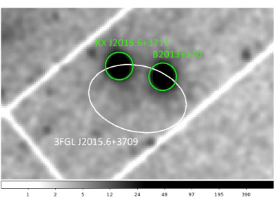
Figure 1: XMM–Newton EPIC-pn 0.3–10 keV image of the field around RX J2015.6$+$3711. The field size is about $12\times 7.5$ arcmin². North is up, east to the left. Both RX J2015.6$+$3711 and the blazar B2013$+$370 were located on CCD 5 and their positions are marked with green circles, each with a radius of 30 arcsec. The white ellipse is centered at $\rm RA=20^{h}15^{m}33\aas@@fstack{s}6$, $\rm Dec=+37^{\circ}10^{\prime}12\aas@@fstack{\prime\prime}2$ (J2000.0) and represents the position (at the 95% confidence level) of the source 3FGL J2015.6$+$3709 in the Fermi Large Area Telescope 4-year point source catalog (Acero et al. 2015; see also Kara et al. 2012). (See the online version of the article for the colour figure.)

We extracted the source photons from a circular region centered at the optical position of the source ($\rm RA=20^{h}15^{m}36\aas@@fstack{s}98$, $\rm Dec=+37^{\circ}11^{\prime}23\aas@@fstack{\prime\prime}2$ (J2000.0); see Halpern et al. 2001) and with a radius of 30 arcsec, to avoid contamination from the closeby blazar. The background was extracted from a similar region, far from the source location and on the same CCD (see Bassani et al. 2014 for an overview of the nearby X-ray emitting sources). We converted the photon arrival times to Solar System barycentre reference frame using the sas task barycen and restricted our analysis to photons having energies between 0.3 and 10 keV. We verified that data were not affected by pile-up through the epatplot script. The 0.3–10 keV average source net count rates are $(2.74\pm 0.02)\times 10^{-1}$, $(8.98\pm 0.09)\times 10^{-2}$ and $(8.83\pm 0.09)\times 10^{-2}$ counts s^-1 for the pn, MOS 1 and MOS 2, respectively.

We applied the standard filtering procedure in the extraction of the spectra, retaining only events optimally calibrated for spectral analysis (flag = 0) and with pattern $\leq 4(12)$ for the pn (MOS) data. We generated the corresponding redistribution matrices and ancillary response files with the rmfgen and arfgen tools, respectively, and grouped the background-subtracted spectra to have at least 100 counts in each spectral bin.

Figure 2: 0.3–10 keV background-subtracted and exposure-corrected light curve of RX J2015.6$+$3711 obtained with the XMM–Newton EPIC cameras with a binning time of 800 s.

2.1.1 Timing analysis

The 0.3–10 keV background-subtracted and exposure-corrected light curve of RX J2015.6$+$3711 is reported in Fig. 2. It was generated by combining the time series from the EPIC cameras during the periods when all three telescopes acquired data simultaneously, using the epiclccorr tool of sas and other tasks in the ftools package (Blackburn 1995). The light curve clearly shows a periodic modulation. We computed a Fourier transform of the pn light curve and found indeed a prominent peak at a frequency of $\sim 1.39\times 10^{-4}$ Hz (at a significance level of about 27$\sigma$, estimated taking into account the presence of the underlying white noise component and the number of independent Fourier frequencies examined in the power spectrum; see the left-hand panel of Fig. 3). A search for periodicities at millisecond periods was precluded owing to the temporal resolution of the pn camera in full frame readout mode, which implies a Nyquist limiting frequency of about 6.8 Hz. We show in the inset of Fig. 3 the Fourier power spectral density of RX J2015.6$+$3711, produced by calculating the power spectrum into 2405 s-long consecutive time intervals, averaging the 48 spectra so evaluated and rebinning geometrically the resulting spectrum with a factor 1.05. A closer inspection of the power spectrum around the frequency of the main peak revealed excess of power up to the second harmonic and also at frequencies of about $9.4\times 10^{-5}$, $1.20\times 10^{-4}$, $1.65\times 10^{-4}$ and $2.55\times 10^{-4}$ Hz (in all cases at a significance level larger than $6\sigma$; see the right-hand panel of Fig. 3). The power spectra filtered in different energy intervals show no evidence for significant peaks above $\sim 3$ keV.

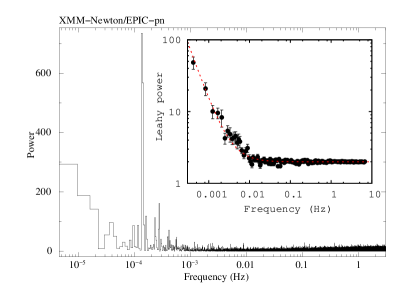
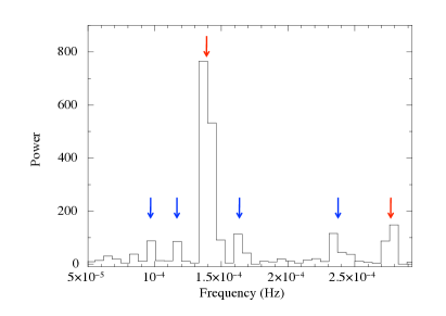
Figure 3: Left-hand panel: 0.3–10 keV power spectrum of RX J2015.6$+$3711 obtained from XMM–Newton EPIC-pn data. Inset: Fourier power spectral density of RX J2015.6$+$3711. The red dashed line represents the modeling of the white and red noise components, i.e. the sum of a constant and a power law function: $P(\nu)=K+C\nu^{-\beta}$, with $K=1.99(1)$ Hz^-1 and $\beta=1.59(8)$. Right-hand panel: 0.3–10 keV power spectrum of RX J2015.6$+$3711 restricted to the frequency range between $5\times 10^{-5}$ and $3\times 10^{-4}$ Hz. The main peak and that of the second harmonic are highlighted with red arrows, whereas the other significant power peaks are marked with blue arrows. All these peaks are detected at a significance level above $6\sigma$ (see the text). (See the online version of the article for the colour figure.)

To refine our period estimate for the main peak in the power spectrum, we performed an epoch-folding search of the light curve by binning the profile into 16 phase bins and searching with a period resolution of 13 s. We then fitted the peak in the $\chi^{2}$ versus trial period distribution as described by Leahy (1987) and derived a best period $P=7196\pm 11$ s (at the 90% confidence level), consistent within the errors with that reported (independently) by Halpern & Thorstensen (2015).

The pn light curve folded on $P$ is shown in the left-hand panel of Fig. 4. The profile is asymmetric and is characterized by a prominent peak in the phase interval $\sim 0.1-0.4$, followed by a minimum in the $0.6-0.9$ range. We also produced an energy versus phase image by binning the source counts into 100 phase bins and 100-eV wide energy channels and normalizing to the phase-averaged energy spectrum and pulse profile. A lack of counts is evident at energy $\lesssim 2$ keV and in the phase interval corresponding to the minimum of the profile (see again the left-hand panel of Fig. 4).

The profiles are approximately phase-aligned at different energies within statistical uncertainties, but their morphology changes as a function of energy (see the middle panel of Fig. 4). In particular we observe a secondary hump in the phase interval 0.8–1.1 in the softest band (0.3–1 keV), a feature that is nearly absent in the 1–2 keV interval. To assess the significance of the observed pulse shape variations as a function of energy, we compared the 0.3–1 keV and 1–2 keV folded profiles using a two-sided Kolmogorov–Smirnov test (Peacock 1983; Fasano & Franceschini 1987). The result shows that the difference between these energy ranges is highly significant: the probability that the two profiles do not come from the same underlying distribution is in fact $\sim 4\times 10^{-7}$, corresponding to a significance of $\sim 5.3\sigma$.

We also analyzed the temporal evolution of the pulse shape in the 0.3–10 keV energy band by dividing the entire duration of the pn observation into four consecutive time intervals, each of length 4$P$, and folding the corresponding light curves on $P$. As shown in the right-hand panel of Fig. 4, the shape of the profile clearly changes as time elapses.

We evaluated the pulsed fractions by fitting a constant plus two sinusoidal functions to the 32-bin folded light curves and considering the semi-amplitude measured from the fundamental frequency component (the sinusoidal periods were fixed to those of the fundamental and second harmonic components). The inclusion of higher harmonic components in the fits was not statistically needed, as determined by means of an $F$–test. The 0.3–10 keV pulsed fractions are $29\pm 1$, $29\pm 2$ and $30\pm 2$% for the pn, MOS 1 and MOS 2 data sets, respectively (uncertainties are reported at the 90% confidence level). The amplitude of the modulation decreases as the energy increases: for pn data we calculated pulsed fractions of $62\pm 4$, $44\pm 2$, $22\pm 3$, $17\pm 3$ and $9\pm 4$% in the 0.3–1, 1–2, 2–3, 3–5 and 5–10 keV energy ranges, respectively. The pulsed fraction is however consistent with the average value over the entire duration of the observation.

In Fig. 5 we show the 0.3–10 keV profiles folded at the best periods corresponding to the frequencies $1.20\times 10^{-4}$ and $1.65\times 10^{-4}$ Hz (i.e. $8332\pm 14$ s and $6052\pm 6$ s, respectively). The modulation amplitudes are $6\pm 1$ and $8\pm 1$%, respectively.

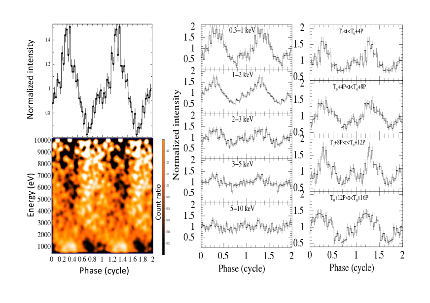
Figure 4: Left-hand panel, top: 0.3–10 keV background-subtracted and exposure-corrected light curve of RX J2015.6$+$3711 (from XMM–Newton/EPIC-pn data) folded on the period $P$=7196 s and sampled in 32 phase bins. Epoch T₀=57 005.6889669 MJD was used as reference. Left-hand panel, bottom: normalized energy versus phase image for the pn data of RX J2015.6$+$3711 (see the text for details). Middle panel: 32-bin pulse profiles in five different energy bands. Energy increases from top to bottom. Right-hand panel: 32-bin pulse profiles in four different time intervals (0.3–10 keV). Time increases from top to bottom. Two cycles are shown in all cases for better visualization. (See the online version of the article for the colour figure.)

Figure 5: 0.3–10 keV background-subtracted and exposure-corrected light curve of RX J2015.6$+$3711 folded on the periods $P$=8332 s (upper panel) and $P$=6054 s (lower panel), and sampled in 16 phase bins. Two cycles are shown for better visualization.

2.1.2 Phase-averaged spectral analysis

We fitted the spectra of the three EPIC cameras together in the 0.3–10 keV energy range using the xspec spectral fitting package (v. 12.9.0; Arnaud 1996). We adopted a set of different single-component models: a blackbody (bbodyrad in xspec notation), an optically-thin thermal bremsstrahlung, an accretion disk consisting of multiple blackbody components (diskpbb) and a power law (pegpwrlw). To describe the absorption by the interstellar medium, we used the Tuebingen-Boulder model (tbabs), with photoionization cross-sections from Verner et al. (1996) and solar chemical abundances from Wilms, Allen & McCray (2000). We included an overall normalization factor to account for calibration uncertainties among the three different X-ray detectors and tied up all the parameters across the three data sets. In the following we will quote all the uncertainties at a 90% confidence level for a single parameter of interest ($\Delta\chi^{2}=2.706$), unless otherwise specified.

A blackbody model is rejected by the data ($\chi^{2}_{\nu}=5.2$ for 368 degrees of freedom; dof hereafter). The bremsstrahlung model yields $\chi^{2}_{\nu}=1.54$ for 368 dof, with the temperature pegged to the highest allowed value of 200 keV. In the disk model, the temperature is allowed to have a radial dependence, $T(r)\propto r^{-p}$. Fixing $p$ to 0.75 (i.e., reproducing the standard geometrically thin and optically thick accretion disk of Shakura & Sunyaev 1973) gives $\chi^{2}_{\nu}=1.30$ for 368 dof. If we leave this parameter free to vary we obtain $\chi^{2}_{\nu}=1.18$ for 367 dof, with $p=0.68^{+0.01}_{-0.02}$. An $F$-test gives a chance probability of $\sim 1.1\times 10^{-9}$, corresponding to a 6.3$\sigma$ improvement. However, the inferred value for the temperature at the inner radius of the disk is $\gtrsim 5.9$ keV, which is quite implausible. We find instead $\chi^{2}_{\nu}=1.19$ for 368 dof for the power law model. However, structured residuals are clearly visible at energy $\lesssim 0.6$ keV and around 6.6 keV. The inclusion of a partial covering absorber (pcfabs), accounting for additional partial absorption, and a Gaussian feature (gauss) in emission, leads to an improvement in the shape of these residuals and to a more satisfactory modeling of the data (see Fig. 6). We obtain $\chi^{2}_{\nu}=0.97$ for 363 dof. The best-fitting parameters are listed in Table 2. The interstellar absorption column density, $\hbox{$N_{\rm H}$}_{,\rm{ISM}}\sim 2\times 10^{21}$ cm^-2, is about one order of magnitude lower than the total Galactic value in the direction of the source ($\sim 1.25\times 10^{22}$ cm^-2; Willingale et al. 2013), implying a closeby location of this source within our Galaxy. The nearby source CTB 87, believed to be at a distance of about 6.1 kpc, has a much higher $N_{\rm H}$ value of $1.4\times 10^{22}$ cm^-2 (Matheson et al. 2013), further supporting the closer distance of this source. The partial ($\approx 83$%) column density is larger than the interstellar column density by a factor of $\sim 3$ (see Table 2), suggesting that the majority of the contribution to the observed absorption is due to an absorber localized close to the source. The broad emission feature around 6.6 keV is suggestive of different contributions, in particular thermal and fluorescent iron lines. The 0.3–10 keV unabsorbed flux is ($3.16\pm 0.05$) $\times 10^{-12}$ erg cm^-2 s^-1.

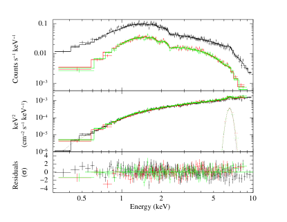
Figure 6: 0.3–10 keV average spectrum of RX J2015.6$+$3711 extracted from XMM–Newton EPIC data. The solid line represents the best-fitting model, i. e. the superposition of an absorbed power law and a Gaussian feature in emission. $E^{2}\times f(E)$ unfolded spectra (middle panel) and post-fit residuals in units of standard deviations (bottom panel) are also shown. Black, red and green colors refer to the pn, MOS 1 and MOS 2 data sets, respectively. (See the online version of the article for the colour figure.)

Table 2: Average spectral fit results for the XMM–Newton observation of RX J2015.6$+$3711. pn and MOSs spectra were fitted together to the tbabs*pcfabs*(pegpwrlw+gauss) model in the 0.3–10 keV energy range. Uncertainties are quoted at the 90% confidence level for a single parameter of interest.

Parameter	Value
$\hbox{$N_{\rm H}$}_{,\rm{ISM}}^{a}$ ($10^{21}$ cm-2)	$2\pm 1$
$\hbox{$N_{\rm H}$}_{,\rm{pcf}}$ ($10^{21}$ cm-2)	$6.1_{-0.7}^{+1.0}$
Covering fraction (%)	$83_{-16}^{+10}$
$\Gamma$	$1.15\pm 0.04$
Energy of line (keV)	$6.61\pm 0.09$
Width of line (keV)	$0.24_{-0.08}^{+0.11}$
Normalization of line ($10^{-6}$ cm-2 s-1)	$5.2_{-1.6}^{+1.9}$
Equivalent width (keV)	$0.18\pm 0.06$
Absorbed fluxb ($10^{-12}$ erg cm-2 s-1)	$2.75_{-0.03}^{+0.05}$
Unabsorbed fluxb ($10^{-12}$ erg cm-2 s-1)	$3.16\pm 0.05$
$\chi^{2}_{\nu}$ (dof)	0.97 (363)
Null hypothesis probability	$6.5\times 10^{-1}$

• The abundances are those of Wilms et al. (2000). The photoelectric absorption cross-sections are from Verner et al. (1996).

• In the 0.3–10 keV energy range.

2.1.3 Phase-resolved spectral analysis

The normalized energy versus phase image relative to the 7196-s periodicity hints at a phase-variable emission, possibly due to a varying absorption along the line of sight (see the left-hand panel of Fig. 4). To better investigate the variability of the X-ray emission along the phase, we computed an hardness ratio between the hard (2–10 keV) and soft (0.3–2 keV) counts along the cycle (see Fig. 7). We then carried out a phase-resolved spectroscopy accordingly, selecting the following four phase intervals: 0.1–0.4 (corresponding to the softest state, around the maximum of the modulation), 0.4–0.6, 0.6–0.9 (related to the hardest state, close to the minimum of the modulation) and 0.9–1.1.

We used all EPIC (pn + MOSs) data and fitted the spectra together to the best-fitting average model. We fixed the interstellar absorption column density, the power law photon index and the centroid and width of the Gaussian feature at the phase-averaged values, after having verified that the lower statistics in the phase-resolved spectra did not allow us to study possible differences for the values of the parameters of the Gaussian feature. We obtained an acceptable $\chi^{2}_{\nu}=1.01$ for 199 dof. Tying up the partial column density across the spectra yielded a significantly worse fit ($\chi^{2}_{\nu}=1.50$ for 202 dof). Therefore, as shown in Table 3, the variability of the X-ray emission along the phase cycle can be successfully ascribed to changes in both the density and spatial extension of the localized absorbing material, and the power law normalization. In particular, the partial column density is significantly larger at the minimum (about $1.2\times 10^{22}$ cm^-2) than at the maximum ($\sim 2.8\times 10^{21}$ cm^-2). Unabsorbed 0.3–10 keV fluxes are ($2.77\pm 0.10$) and ($3.62\pm 0.09$) $\times 10^{-12}$ erg cm^-2 s^-1, respectively (see Table 3). The phase-resolved spectra together with the best-fitting model are shown in the right-hand panel of Fig. 7 (only for pn data for plotting purpose).

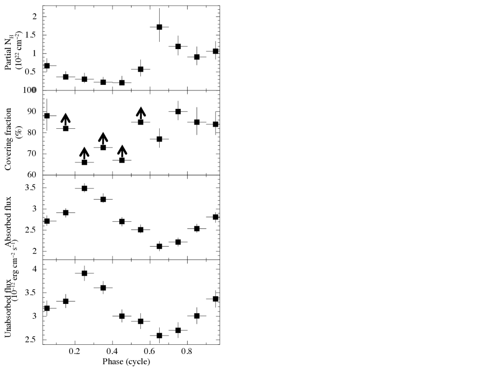
Figure 8: Evolution of the column density and covering fraction of the partial absorber and of the 0.3–10 keV fluxes as a function of the phase for the XMM–Newton observation of RX J2015.6$+$3711. The 10 pn spectra (each corresponding to a 0.1-wide phase interval) were fitted together to the tbabs*pcfabs*(pegpwrlw+gauss) model in the 0.3–10 keV energy range (see the text for details). Uncertainties and lower limits (indicated by arrows) are reported at a 90% confidence level for a single parameter of interest.

To better characterize the phase-dependence of the parameters, we repeated the analysis (only for pn data) by dividing the phase cycle into 10 equal intervals, each of width 0.1 in phase, and fitting the corresponding spectra together to the same model as above. We obtained $\chi^{2}_{\nu}=0.96$ for 404 dof. The evolution of the parameters and the fluxes along the cycle is shown in Fig. 8. An anti-correlation between the partial absorption column density and the X-ray intensity can be seen in the figure.

Table 3: Phase-resolved spectral fit results for the XMM–Newton observation of RX J2015.6$+$3711. pn and MOSs spectra were fitted together to the tbabs*pcfabs*(pegpwrlw+gauss) model in the 0.3–10 keV energy range. The interstellar absorption column density and the power law photon index were fixed at the phase-averaged values, resulting in $\chi^{2}_{\nu}=1.01$ for 199 dof (see the text). Uncertainties and lower limits are quoted at a 90% confidence level for a single parameter of interest.

Phase range	$\hbox{$N_{\rm H}$}_{,\rm{pcf}}$	Cvfa	Abs fluxb	Unabs fluxb
	($10^{21}$ cm-2)	(%)	($10^{-12}$ erg cm-2 s-1)
$0.1-0.4$ (max)	$2.8_{-0.4}^{+0.8}$	$\gtrsim 81$	$3.23_{-0.06}^{+0.07}$	$3.62\pm 0.09$
$0.4-0.6$	$3.2_{-0.6}^{+1.3}$	$\gtrsim 77$	$2.62_{-0.08}^{+0.09}$	$2.95_{-0.10}^{+0.11}$
$0.6-0.9$ (min)	$12.0\pm 0.2$	$84\pm 3$	$2.30_{-0.06}^{+0.07}$	$2.77\pm 0.10$
$0.9-1.1$	$8.2_{-0.1}^{+0.2}$	$86_{-4}^{+5}$	$2.78_{-0.09}^{+0.08}$	$3.27\pm 0.12$

• Covering fraction of the partial absorber.

• In the 0.3–10 keV energy range.

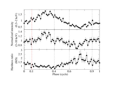
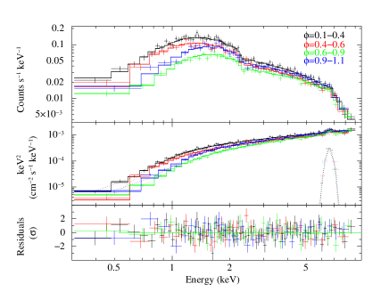
Figure 7: Left-hand panel: 64-bin pulse profile of RX J2015.6$+$3711 in two different energy intervals. The hardness ratio between the hard and soft bands is also plotted at the bottom. The red vertical dashed lines indicate the phase ranges used for the phase-resolved spectral analysis. Right-hand panel: phase-resolved spectra of RX J2015.6$+$3711 extracted from XMM–Newton EPIC-pn data. The solid lines represent the best-fitting model to the data (a power law plus a Gaussian feature in emission, both corrected for interstellar and local absorption). $E^{2}\times f(E)$ unfolded spectra (middle panel) and post-fit residuals in units of standard deviations (bottom panel) are also shown. (See the online version of the article for the colour figure).

2.2 Chandra

The Chandra satellite observed RX J2015.6$+$3711 twice, on 2001 Jul 8 and 2010 Jan 16–17 (see Table 1). The first observation (obs. ID 1037; PI: Garmire) was performed with the Advanced CCD Imaging Spectrometer spectroscopic CCD array (ACIS-S; Garmire et al. 2003) set in faint timed-exposure (TE) imaging mode. The total exposure was about 17.8 ks and the source was positioned on the back-illuminated S3 chip. The second observation (obs. ID 11092; PI: Safi-Harb) used instead the imaging CCD array (ACIS- I) operated in very faint TE mode and lasted about 69.3 ks. The source was positioned on the I3 chip.

We analyzed the data following the standard analysis threads with the Chandra Interactive Analysis of Observations software (ciao, v. 4.7; Fruscione et al. 2006) and the calibration files in the Chandra caldb (v. 4.6.9).

The source fell close to the edge of the CCD in the 2001 observation and was very far off-axis in that carried out in 2010 (for both these observations the aim point of the ACIS was indeed the supernova remnant CTB 87, which is located at an angular distance of $\sim 5.2$ arcmin from the nominal position of RX J2015.6$+$3711). Source photons were then collected from a circular region around the source position with a radius of 15 arcsec. Background was extracted from a nearby circle of the same size. We converted the photon arrival times to Solar System barycentre reference frame using the ciao tool axbary and restricted our analysis to photons having energies between 0.3 and 8 keV. The average source net count rates in this band are $(8.5\pm 0.2)\times 10^{-2}$ and $(1.23\pm 0.01)\times 10^{-1}$ counts s^-1 for the first and second observation, respectively.

We created the source and background spectra, the associated redistribution matrices and ancillary response files using the specextract script. We grouped the background-subtracted spectra to have at least 30 and 100 counts in each spectral bin for the first and second observation, respectively.

2.2.1 Timing analysis

Very recently, timing analysis of the longest Chandra observation (obs. ID 11092) unveiled the presence of the 2-hr periodicity observed in the XMM–Newton  data (Halpern & Thorstensen 2015). The energy-dependent light curves folded on this period closely resemble the profiles derived from the XMM–Newton observation (see e.g. Fig. 17 of Halpern & Thorstensen 2015), with a modulation amplitude that decreases as the energy increases. We confirmed this detection in the soft X-ray band (0.5–2 keV) and verified that, except for the harmonic, the other periodicities discovered in the XMM–Newton observation are not visible, likely due to the lower counting statistics in the Chandra data sets.

Our searches for periodicities in the data of the other observation (obs. ID 1037) were instead inconclusive. Only one power peak is visible and we note that it is coincident with the frequency of known artificial signal due to the source dithering off the chip at regular time intervals.

2.2.2 Spectral analysis

The values for the source net count rate translate into a pile-up fraction of about 10 and 15% for the first and the second observation, respectively, as estimated with pimms (v 4.8). We then accounted for possible spectral distortions using the model of Davis (2001), as implemented in xspec, and following the recommendations in ‘The Chandra ABC Guide to Pile-up’. We fitted the two spectra together in the 0.3-8 keV energy range with an absorbed power law model and all the parameters left free to vary. However, the column density was compatible between the two epochs at the 90% confidence level and thus was tied up. We obtained $\chi^{2}_{\nu}=1.21$ for 118 dof, with $N_{\rm H}$= $(6\pm 1)\times 10^{21}$ cm^-2. The spectrum was harder in 2001 ($\Gamma=0.6\pm 0.1$) than in 2010 ($\Gamma=0.95\pm 0.06$). The emission feature around 6.6 keV is not detected, likely due to the lower statistics compared to the XMM–Newton data sets. The addition of a Gaussian feature in emission with parameters fixed at the values derived from the XMM–Newton observation (see Table 2) yields upper limits for the equivalent width of 52 and 119 eV in 2001 and 2010, respectively (at a 90% confidence level). The 0.3–10 keV unabsorbed fluxes at the two epochs were $(9.0\pm 0.6)\times 10^{-12}$ and $(4.05\pm 0.09)\times 10^{-12}$ erg cm^-2 s^-1. The soft X-ray flux of RX J2015.6$+$3711 was thus larger in 2001 than in 2010 and 2014 (the epoch of the XMM–Newton observation) by a factor of $\sim 2.2$ and $\sim 2.8$, respectively.

2.3 Swift

Our analysis of Swift data is mainly aimed at comparing the simultaneous soft X-ray and ultraviolet/optical fluxes of RX J2015.6$+$3711 at different epochs. Therefore, we focus here on the two longest observations of the source (obs IDs: 00035639003, 00041471002; see Table 1). The X-ray Telescope (XRT; Burrows et al. 2005) was set in photon counting mode in both cases.

We processed the data with standard screening criteria and generated exposure maps with the task xrtpipeline (v. 0.13.1) from the ftools package. We selected events with grades 0–12 and extracted the source and background event files using xselect (v. 2.4). We accumulated the source counts from a circular region centered at the peak of the source point-spread function and with a radius of 20 pixels (one XRT pixel corresponds to about 2.36 arcsec). To estimate the background, we extracted the events within a circle of the same size sufficiently far from the blazar and other point sources.

We created the observation-specific ancillary response files (using exposure maps) with xrtmkarf, thereby correcting for the loss of counts due to hot columns and bad pixels and accounting for different extraction regions, vignetting and PSF corrections. We then assigned the redistribution matrices v012 and v014 available in the heasarc calibration database to the 2006 and 2010 data sets, respectively. We grouped the spectral channels to have at least 20 counts in each spectral bin and fitted in the 0.3 to 10 keV energy interval with an absorbed power law model. The inferred 0.3-10 keV unabsorbed fluxes are $\sim 6.9$ and $4.1\times 10^{-12}$ erg cm^-2 s^-1 in 2006 and 2010, respectively. This is in line with a fading trend of the source in about 10 yr.

3 UV/optical observations and data analysis

RX J2015.6$+$3711 was not positioned on the detectors of the XMM–Newton Optical/UV Monitor telescope (Mason et al. 2001) throughout the observation. We thus focused on the two observations by the Ultra-violet and Optical Telescope (UVOT; Roming et al. 2005) aboard Swift, which lasted about 7.0 and 7.2 ks, respectively, and were carried out in image mode. All the available filters were used in both cases (see Table 4), providing a wavelength coverage within the 1700–6000 Å range. We performed the analysis for each filter and on the stacked images. First, we ran the uvotdetect task and found the UV and optical counterpart of RX J2015.6$+$3711 at position $\rm RA=20^{h}15^{m}36\aas@@fstack{s}959$, $\rm Dec=+37^{\circ}11^{\prime}22\aas@@fstack{\prime\prime}70$ (J2000.0), which is compatible with the location reported by Halpern et al. (2001) within the errors. We then used the uvotsource command, which calculates detection significances, count rates corrected for coincidence losses and dead time of the detector, flux densities and magnitudes through aperture photometry within a circular region, and applies specific corrections due to the detector characteristics. We adopted an extraction radius of 5 and 3 arcsec for the UV and optical filters, respectively, and applied the corresponding aperture corrections. The derived values for the absorbed magnitudes at the two different epochs are listed in Table 4 (magnitudes are expressed in the Vega photometric system; see Poole et al. 2008 for more details and Breeveld et al. 2010, 2011 for the most updated zero-points and count rate-to-flux conversion factors). The source is brighter in all bandpasses in 2006 than in 2010, confirming the fading of the source also in the optical and UV.

To estimate the X-ray–to–optical flux ratio at the two different epochs of the Swift observations, we determined the unabsorbed 2–10 keV fluxes measured by the XRT and considered the values for the $V$-band magnitudes observed by the UVOT (central wavelength of 5468 Å and full-width at half-maximum of 769 Å). Adopting the value of the interstellar hydrogen column density derived from our model fit to the phase-averaged X-ray spectrum, and a conversion factor of $\hbox{$N_{\rm H}$}/A_{\rm V}$ of $(2.87\pm 0.12)\times 10^{21}$ cm^-2 mag^-1 (according to the relation of Foight et al. 2015), we estimated an optical extinction $A_{\rm V}=0.60\pm 0.12$ mag. We note that this value is lower than the integrated line-of-sight optical extinction at the position of the source, $A_{\rm V}\sim 5.0$ mag, computed according to the recalibration (Schlafly & Finkbeiner 2011) of the extinction maps from Schlegel, Finkbeiner & Davis (1998). Using the Vega magnitude-to-flux conversion, we inferred dereddened $V$-band fluxes for the source of $(4.6\pm 0.8)\times 10^{-12}$ erg cm^-2 s^-1 in 2006 and $(2.3\pm 0.4)\times 10^{-12}$ erg cm^-2 s^-1 in 2010. The X-ray–to–optical flux ratio is then $F_{\mathrm{X}}/F_{\mathrm{V}}=1.4\pm 0.2$ and $1.7\pm 0.2$, respectively (at the 1$\sigma$ confidence level), thus compatible between the two epochs.

Table 4: Swift UVOT observations of RX J2015.6$+$3711 at two different epochs. Magnitudes are in the Vega photometric system and are not corrected for interstellar extinction. Uncertainties are quoted at a 1$\sigma$ confidence level, whereas upper limits are given at a 3$\sigma$ confidence level.

Filter	Date	Exposure	Magnitude
		(s)	(mag)
$UVW2$	2006 Nov 17	2421	$19.76\pm 0.14$
	2010 Aug 6–10	944	$19.96\pm 0.25$
$UVM2$	2006 Nov 17	1567	$19.83\pm 0.21$
	2010 Aug 6–10	4940	$21.22\pm 0.36$
$UVW1$	2006 Nov 17	1210	$18.51\pm 0.09$
	2010 Aug 6–10	629	$>19.98$
$U$	2006 Nov 17	598	$17.65\pm 0.06$
	2010 Aug 6–10	298	$18.95\pm 0.14$
$B$	2006 Nov 17	598	$18.00\pm 0.05$
	2010 Aug 6–10	236	$19.28\pm 0.14$
$V$	2006 Nov 17	598	$17.19\pm 0.06$
	2010 Aug 6–10	182	$17.94\pm 0.13$

4 Discussion

Based on the wealth of observations we have collected for RX J2015.6$+$3711, from the optical to the X-rays, we can now explore the possibility that this source indeed belongs to the class of mCVs, as proposed by Halpern & Thorstensen (2015).

4.1 The X-ray periodicities and the accretion geometry

The X-ray properties of mCVs are strongly related to the accretion flow onto the WD. The accretion configuration is different for the two subclasses of mCV: in polars the high magnetic fields prevent the formation of an accretion disk and material flows in a column-like funnel; in IPs matter accretes either via a truncated disc (or ring; Warner 1995) or via a stream as in the polars (the diskless accretion model first proposed by Hameury, King & Lasota 1986). Whether the disk forms, or not, close to the WD surface, the infalling material is magnetically channeled towards the polar caps, resulting in emission strongly pulsed at the spin period of the accreting WD in disk accretors or at the beat period in disk-less accretors. Matter is de-accelerated as it accretes, and a strong standing shock develops in the flow above the WD surface. X-rays are then radiated from the post-shock plasma.

Within the mCV scenario, the $\sim$ 2-hr modulation discovered in the X-ray (0.3–10 keV) emission of RX J2015.6$+$3711 (see 2.1.1) can be naturally interpreted as the trace of the accreting WD spin period. The spin modulation has a highly structured shape that resembles those observed in IPs rather than in polars, which show instead a typical on/off behaviour due to self occultation of the accreting pole and thus alternate bright and faint phases (see Warner 1995; Matt et al. 2000 for the prototypical polar; Ramsay et al. 2009, Traulsen et al. 2010 and Bernardini et al. 2014 for more recent studies). The modulation has a large amplitude (about 30%) and the detection of the second harmonic suggests that accretion occurs onto two polar regions located at the opposite sides of the WD surface, and both visible. The main accreting pole produces the sinusoidal modulation, whereas the other pole is responsible for the secondary hump observed around the minimum of the spin pulse profile (see Fig. 4). The relative contribution of the two poles to the observed emission can be quantitatively estimated from the fundamental-to-second harmonic amplitude ratio, which is $\sim 3$ for this system.

The additional weaker periodicities detected in the power spectrum can be identified as the orbital sidebands of the spin pulse in an IP system. Theory predicts that, if accretion onto the WD occurs via a funnel rather than a disk, the asynchronous rotation of the WD should produce modulation not only at the spin frequency ($\omega$), but also at the orbital ($\Omega$) and beat ($\omega$ – $\Omega$) frequencies. Higher harmonics of the beat frequency may be present for specific combinations of the system inclination and the offset angle between the magnetic and spin axes (see Wynn & King 1992). Setting the spin frequency as $\omega=1.39\times 10^{-4}$ Hz, the frequencies $9.4\times 10^{-5}$, $1.20\times 10^{-4}$, $1.65\times 10^{-4}$ and $2.6\times 10^{-4}$ Hz (at which excess of power is observed, see 2.1.1) would correspond to the sideband frequencies $\omega$ – 2$\Omega$, $\omega$ – $\Omega$, $\omega$ + $\Omega$ and 2$\omega$ – $\Omega$, respectively, for a putative binary orbital frequency $\Omega\sim 2.26\times 10^{-5}$ Hz (i.e. an orbital period $P_{{\rm orb}}\sim 12$ hr). We note that the X-ray power spectrum does not show any evident signal at this putative period, which is not surprising given the low amplitude of the sideband $\omega$ – $\Omega$ and $\omega$ + $\Omega$ signals ($\sim 6$ and 8%, respectively).

Although the prominent peak at the spin frequency in the X-ray power spectrum implies that accretion occurs predominantly through a Keplerian disk (the circulating material loses all knowledge of the orbital motion; see Wynn & King 1992), the detection of the orbital sidebands suggests that a non negligible fraction of matter leaps over the disk and is directly channeled onto the WD magnetic poles within an accretion column. This sort of hybrid accretion mode, dubbed ‘disk-overflow’, is supported by theoretical simulations (see e.g. Armitage & Livio 1998) and it has been observed in other confirmed IPs (see Bernardini et al. 2012, and references therein). The spin-to-beat amplitude ratio of $4.8\pm 0.4$ (at the 90% confidence level) implies that approximately 80% of matter is accreted through the disk-fed mode.

The spin modulation amplitude decreases as the energy increases (the pulsed fraction is only about 9% above 5 keV). This behaviour is typical for IPs. In these systems the softest X-rays are more prone to absorption from neutral material in the pre-shock flow, whereas X-rays at higher energies are essentially unaffected by photo-electric absorption, resulting in a decrease of the modulation amplitude (Rosen, Mason & Cordova 1988). Furthermore, the overall pulse shape changes with time (see the right-hand panel of Fig. 4), in particular the intensity of the secondary peak increases. Such variations are also observed in a few similar systems (e.g. Bernardini et al. 2012; Hellier 2014), and are likely due to the different accretion modes occurring in these binaries.

4.2 The X-ray spectral properties

The average X-ray spectrum of RX J2015.6$+$3711 can be described by an absorbed hard power law ($\Gamma=1.15\pm 0.04$) plus a broad ($\sim 0.25$ keV) Gaussian emission feature at $6.61\pm 0.09$ keV. The absorption is provided by the interstellar medium component (with column density $\hbox{$N_{\rm H}$}_{,\rm{ISM}}\sim 2\times 10^{21}$ cm^-2) plus a thicker ($\hbox{$N_{\rm H}$}_{,\rm{pcf}}\sim 6\times 10^{22}$ cm^-2) absorber partially covering the X-ray emitting regions. A partial covering absorption and the iron complex are nevertheless defining properties of mCVs (e.g., Yuasa et al. 2010; Girish & Singh 2012; Ezuka & Ishida 1999). The large width for the line is suggestive of both thermal and fluorescent contributions (i.e. the 6.67 keV He-like and the 6.97 keV H-like lines, plus the 6.4 keV fluorescent line). In particular the fluorescent line is produced by reflection of X-rays from cold matter that could be the WD surface or the pre-shock flow.

We observe a conspicuous hardening at the minimum of the rotational phase cycle and we find that the phase-variable emission can be accounted for mainly by changes in the amount of local absorbing material and the power law normalization. Moreover, the partial column density is anti-correlated with the X-ray flux along the cycle. The variability in the extension of the local absorber (covering fraction) is instead less significant and only lower limits can be inferred around the maximum of the modulation. Although localised absorption is also detected in the X-ray light curves of polars, this is generally pronounced during the bright phase where the typical dips are due to absorption when the accretion column points towards the observer.

The spectral changes along the modulation phase in RX J2015.6$+$3711 are typically observed in IPs and can be explained within the accretion curtain scenario presented by Rosen et al. (1988). According to their model, the modulation is mainly caused by spin-dependent photoelectric absorption from pre-shock material flowing from the disk towards the polar caps in arc-shaped structures extending above the WD. In this context, the spin-phase modulation of RX J2015.6$+$3711 in the soft X-rays likely reflects changes in the absorption along the curtains. At the minimum of the rotational phase the softest X-ray photons from the WD surface are highly absorbed, resulting in a spectral hardening and a decrease in the amount of emission. On the other hand, at the maximum of the modulation, the absorption is less efficient and the radiation intensity will be larger.

4.3 The long-term X-ray variability and multiwavelength emission

RX J2015.6$+$3711 appears to have gradually faded in the X-rays since 2001 (see 2.2 and 2.3), a behaviour that is not uncommon in mCVs of the IP type (Warner 1995).

The simultaneous X-ray and UV/optical observations of RX J2015.6$+$3711 carried out with Swift enable a straight estimate of the flux in different energy bands (see Section 3). The source appears to be brighter in 2006 November than in 2010 August in all bands. The ratio between the unabsorbed X-ray and optical flux is roughly the same at the two epochs: $F_{\mathrm{X}}/F_{\mathrm{V}}\sim 1.4-1.7$. If we interpret the X-ray luminosity as accretion luminosity, the rather stable ratio suggests that both the X-ray and optical luminosities are tracing changes in the mass accretion rate. Moreover, a relatively low value for the ratio is not surprising for the CVs, which have X-ray–to–optical flux ratios much lower with respect to LMXBs (see van Paradijs & Verbunt 1984; Patterson & Raymond 1985; Motch et al. 1996), with the mCVs showing higher ratios compared to non-magnetic systems (see Verbunt et al. 1997). Therefore, both the intrinsic emission of the disk and the X-ray reprocessed radiation provide an important contribution to the UV and optical emission in these systems.

4.4 The system parameters

The 2-hr spin pulsations pin down RX J2015.6$+$3711 as the second slowest rotating WD in the class of IPs (after RX J0524+4244, also known as "Paloma", with $P_{\rm spin}\sim 2.3$ hr; see Schwarz et al. 2007). If the additional peaks detected in the X-ray power spectrum are indeed the orbital sidebands, then the estimated orbital period of the system of about 12 hr would imply a degree of asynchronism $P_{{\rm spin}}/P_{\rm{orb}}\sim 0.16$, which is larger than that observed for most of the long-orbital period IPs (Norton et al. 2004; Bernardini et al. 2012; see also the catalogue available at the Intermediate Polar Home Page). Taken at face value, the long spin period would be peculiar when compared to other slow rotators which are all short orbital period systems, including the IP Paloma.

For a system with orbital period of about 12 hr, the likely companion would be a G- or early K-type star (Smith & Dhillon 1998). Adopting an absolute magnitude in the $K$-band in the range 3.50–4.51 mag (Bilir et al. 2008), using the value for the $K$-band magnitude of RX J2015.6$+$3711 ($14.79\pm 0.15$ mag), and assuming that the donor star in this binary system totally contributes at these wavelengths, the estimated distance would be in the range 1–2 kpc, with no intervening absorption. Our estimate does not change significantly if the effects of interstellar absorption are considered, since adopting the optical reddening derived in Section 3 and the extinction coefficients at different wavelengths of Fitzpatrick (1999), the inferred absorption in this band is only $A_{\rm K}\sim 0.07$ mag.

5 Conclusions

A deep XMM–Newton observation of RX J2015.6$+$3711, together with archival Chandra and Swift observations, allowed us to unambiguously identify this source with a magnetic cataclysmic variable.

Although we did not detect directly the orbital period of the system, several properties point toward the intermediate polar identification, and the 2 hr modulation as the white dwarf spin period. In particular, no coherent signal is observed at shorter periods (ruling out the presence of a lower spin period), and the presence of additional weaker periodicities close to the most significant one at 2 hr could be reconciled with orbital sidebands for a putative orbital period of about 12 hr. In this case the system would be an intermediate polar with an anomalous spin–to–orbit period ratio for its long orbital period. Alternatively, the orbital period could be one of the sideband periods itself, and in this case RX J2015.6$+$3711  would resemble systems like Paloma (Schwarz et al. 2007) or IGR J1955$+$0044 (Bernardini et al. 2013), which are characterized by a high spin–to–orbit period ratio ($P_{{\rm spin}}/P_{\rm{orb}}\sim 0.9$) and are believed to be intermediate polars (or pre-polars) on their way to reach synchronism.

Both the shape and the spectral characteristics of the 2 hr modulation are typical of the intermediate polars. Furthermore, the amplitudes of the different modulations indicate that accretion takes place onto the two polar caps mostly through a truncated disk (about 80%), with a non negligible contribution from an accretion stream, again a peculiarity shared by several intermediate polars.

Further optical observations are planned to shed light on the exact orbital period of this intriguing system, which in any case appears to play a key role in understanding of the evolution of magnetic cataclysmic variables.

References

- [Acero et al. (2015)] Acero F. et al., 2015, ApJS, 218, 23
- [Armitage & Livio (1998)] Armitage P. J., Livio M., 1998, ApJ, 493, 898
- [Arnaud (1996)] Arnaud K. A., 1996, in Jacoby G. H., Barnes J., eds, ASP Conf. Ser. Vol. 101, Astronomical Data Analysis Software and Systems V. Astron. Soc. Pac., San Francisco, p. 17
- [Bassani (2014)] Bassani L., Landi R., Malizia A., Stephen J. B., Bazzano A., Bird A. J., Ubertini P., 2014, A&A, 561, 108
- [Bernardini et al. (2012)] Bernardini F., de Martino D., Falanga M., Mukai K., Matt G., Bonnet-Bidaud J.-M., Masetti N., Mouchet M., 2012, A&A, 542, 22
- [Bernardini et al. (2013)] Bernardini F. et al., 2013, MNRAS, 435, 2822
- [Bernardini et al. (2014)] Bernardini F., de Martino D., Mukai K., Falanga M., 2014, MNRAS 445,1403
- [Bernardini et al. (2015)] Bernardini F., de Martino D., Mukai K., Israel G., Falanga M., Ramsay G., Masetti N., 2015, MNRAS, 453, 3100
- [Bilir et al. (2008)] Bilir S., Karaali S., Ak S., Yaz E., Cabrera-Lavers A., Cos kunoglu K. B., 2008, MNRAS, 390, 1569
- [Blackburn (1995)] Blackburn J. K., 1995, in ASP Conf. Ser. 77: Astronomical Data Analysis Software and Systems IV, Shaw R. A., Payne H. E., Hayes J. J. E., eds., pp. 367
- [Bogdanov et al. (2015)] Bogdanov S. et al., 2015, ApJ, 806, 148
- [Breeveld et al. (2010)] Breeveld A. A. et al., 2010, MNRAS, 406, 1687
- [Breeveld et al. (2011)] Breeveld A. A., Landsman W., Holland S. T., Roming P., Kuin N. P. M., Page M. J., 2011, in McEnery J. E., Racusin J. L., Gehrels N., eds, AIP Conf. Proc. Vol. 1358, Gamma Ray Bursts 2010. Am. Inst. Phys., New York, p. 373
- [Burrows et al. (2005)] Burrows D. N. et al., 2005, Space Science Reviews, 120, 165
- [Canizares et al. (2005)] Canizares C. R. et al., 2005, PASP, 117, 1144
- [Davis (2001)] Davis J. E., 2001, ApJ, 562, 575
- [de Martino et al. (2010)] de Martino D. et al., 2010, A&A, 515, 25
- [de Martino et al. (2013)] de Martino D. et al., 2013, A&A, 550, 89
- [de Martino et al. (2015)] de Martino D. et al., 2015, MNRAS, 454, 2190
- [Ezuka & Ishida (1999)] Ezuka H., Ishida M., 1999, ApJS, 120, 277
- [Fasano & Franceschini 1987] Fasano G., Franceschini A., 1987, MNRAS, 225, 155
- [Ferrario et al. 2015] Ferrario L., de Martino D., Gänsicke B. T., 2015, Space Sci. Rev.
- [Fitzpatrick 1999] Fitzpatrick E. L., 1999, PASP, 111, 63
- [Foight et al.2015] Foight D., Güver T., Özel F., Slane P., 2015, ArXiv eprints, arXiv:1504.07274
- [Fruscione et al. (2006)] Fruscione A. et al., 2006, in Silva D. R., Doxsey R. E., eds, Proc. SPIE, Vol. 6270, Observatory Operations: Strategies, Processes, and Systems. SPIE, Bellingham, p. 62701V
- [Garmire et al. (2003)] Garmire G. P., Bautz M. W., Ford P. G., Nousek J. A., Ricker G. R., Jr, 2003, in Truemper J. E., Tananbaum H. D., eds, Proc. SPIE, Vol. 4851, X-Ray and Gamma-Ray Telescopes and Instruments for Astronomy. SPIE, Bellingham, p. 28
- [Girish & Singh (2012)] Girish V., Singh K. P., 2012, MNRAS, 427, 458
- [Halpern et al. (2001)] Halpern J. P., Eracleous M., Mukherjee R., Gotthelf E. V, 2001, ApJ, 551, 1016
- [Halpern & Thorstensen (2015)] Halpern J. P., Thorstensen J. R., 2015, AJ, 150, 170
- [Hameury et al. (1986)] Hameury J.-M., King A. R., Lasota J.-P., 1986, MNRAS, 218, 695
- [Hellier (2014)] Hellier C., 2014, EPJWC, 64, 07001
- [Kara et al. (2012)] Kara E. et al., 2012, ApJ, 746, 159
- [Leahy et al. (1987)] Leahy D. A., 1987, A&A, 180, 275
- [Masetti et al. (2006)] Masetti N. et al., 2006, A&A, 459, 21
- [Mason et al. 2001 (2001)] Mason K. O. et al., 2001, A&A, 365, L36
- [Matheson et al. (2013)] Matheson H., Safi-Harb S., Kothes R., 2013, ApJ, 774, 33
- [Matt et al. (2013)] Matt G., de Martino D., Gänsicke B. T., Negueruela I., Silvotti R., Bonnet-Bidaud J. M., Mouchet M., Mukai K., 2000, A&A, 358, 177
- [Motch et al. (1996)] Motch C., Haberl F., Guillout P., Pakull M., Reinsch K., Krautter J., 1996, A&A, 307, 459
- [Norton et al. (204)] Norton A. J., Wynn G. A., Somerscales R. V., 2004, ApJ, 614, 349
- [Papitto et al. 2013] Papitto A. et al., 2013, Nature, 501, 517
- [Patterson & Raymond 1985] Patterson J. & Raymond J. C., 1985, ApJ, 292, 535
- [Peacock 1983] Peacock J. A., 1983, MNRAS, 202, 615
- [Poole et al. 2008] Poole T. S. et al., 2008, MNRAS, 383, 627
- [Ramsay et al. 2009] Ramsay G., Rosen S., Hakala P., Barclay T., 2009, MNRAS, 395, 416
- [Roming et al. 2005] Roming P. W. A. et al., 2005, Space Science Review, 120, 95
- [Rosen et al. 1988] Rosen S. R., Mason K. O., Cordova F. A., 1988, MNRAS, 231, 549
- [Schlafly & Finkbeiner 2011] Schlafly E. F., Finkbeiner D. P., 2011, ApJ, 737, 103
- [Schlegel et al. 1998] Schlegel D. J., Finkbeiner D. P., Davis M., 1998, ApJ, 500, 525
- [Schwarz et al. 2007] Schwarz R., Schwope A. D., Staude A., Rau A., Hasinger G., Urrutia T., Motch C., 2007, A&A, 473, 511
- [Shakura & Sunyaev et al. 1973] Shakura N. I. & Sunyaev R. A., 1973, A&A, 24, 337
- [Smith et al. 1998] Smith D. A., Dhillon V. S., 1998, MNRAS, 301, 767
- [Stappers et al. 2014] Stappers B. W. et al., 2014, ApJ, 790, 39
- [Strüder et al. 2001] Strüder L. et al., 2001, A&A, 365, 18
- [Thorstensen & Armstrong 2005] Thorstensen J. R., Armstrong E., 2005, AJ, 130, 759
- [Traulsen et al. 2010] Traulsen I., Reinsch K., Schwarz R., Dreizler S., Beuermann K., Schwope A. D., Burwitz, V., 2010, A&A, 516, 76
- [Turner et al. (2001)] Turner M. J. L., 2001, A&A, 365, L27
- [van Paradijs & Verbunt (1984)] van Paradijs J., Verbunt F., 1984, AIPC, 115, 49
- [Verbunt et al. (1997)] Verbunt F., Bunk W. H.; Ritter H., Pfeffermann E., 1997, A&A, 327, 602
- [Verner et al. (1996)] Verner D. A., Ferland G. J., Korista K. T., Yakovlev D. G., 1996, ApJ, 465, 487
- [Warner (1995)] Warner B., 1995, Cambridge Astrophysics Series, 28: Cataclysmic Variable Stars. Cambridge Univ. Press, Cambridge
- [Willingale et al. (2013)] Willingale R., Starling R. L. C., Beardmore A. P., Tanvir N. R., O’Brien P. T., 2013, MNRAS, 431, 394
- [Wilms et al. (2000)] Wilms J., Allen A., McCray R., 2000, ApJ, 542, 914
- [Wynn & King (1992)] Wynn G. A., King A. R., 1992, MNRAS, 255, 83
- [Yuasa et al. (2010)] Yuasa T. et al., 2010, A&A, 520, 25