Generalizing the Frailty Assumptions in Survival Analysis

Abstract

This paper studies Cox’s regression hazard model with an unobservable random frailty where no specific distribution is postulated for the frailty variable, and the marginal lifetime distribution allows both parametric and non-parametric models. Laplace’s approximation method and gradient search on smooth manifolds embedded in Euclidean space are applied, and a non-iterative profile likelihood optimization method is proposed for estimating the regression coefficients. The proposed method is compared with the Expected-Maximization method developed based on a gamma frailty assumption, and also in the case when the frailty model is misspecified.

Keywords: Cox model, Frailty, Local mixture model, Newton’s method, Smooth manifold, Survival analysis.

1 Introduction

Frailty models are important for analyzing survival time data and have been studied by many researchers; for example, Klein (1992), Hougaard (1986), Clayton (1978) and Gorfine et al. (2006). One way of deriving frailty survival models, which we do not follow here, is to formulate the frailty factor as a single parameter, $\theta$, presenting the association between time-to-event data of two correlated events, in which $\theta=1$ is interpreted as being no correlation while $\theta>1$ and $\theta<1$ demonstrate positive and negative association, respectively (Hu et al., 2011; Nan et al., 2006; Clayton and Cuzick, 1985;Clayton, 1978; Oakes, 1982).

An alternative approach for modeling heterogeneity as unobserved covariate, is to add the frailty variable as a multiplicative factor to the baseline hazard function. In Hougaard (1986) a positive stable family is assumed for the frailty variable and the marginal survival time is assumed to have an exponential or Weibull distribution or be unspecified. Various hazard functions, including Cox’s regression model, have been generalized by assuming a gamma frailty variable with mean equal to 1 and variance $\eta$, see Nielsen et al. (1992) and Klein (1992). They utilize the Expectation-Maximization algorithm for estimation of parametric and nonparametric accumulated hazard function and regression coefficients. Further, Gorfine et al. (2006) proposed a different approach for estimation in non-parametric frailty survival models, which is applicable for any parametric model with finite mean on the frailty variable.

Although, different models have been assumed for the multiplicative frailty variable, (Gorfine et al., 2006; Hougaard, 1984; Hougaard, 1986), one of the most frequently used distributions is the gamma distribution, because of its tractable properties (Klein, 1992; Nielsen et al., 1992; Vaupel et al., 1979). For example Martinussen et al. (2011) used gamma frailty in the Aalen additive model, and Zeng et al. (2009) studied transformation models with gamma frailty for multivariate survival analysis, in which $\eta=0$ (no frailty) is also allowed. In addition, Abbring and Van Den Berg (2007) establish the fact that conditional frailty among survivors is always gamma distributed if and only if the frailty distribution is regularly varying at zero.

In this paper, we consider Cox’s regression model (Cox, 1972) with a multiplicative frailty factor on which no specific model is imposed, as biased estimators might be obtained if the frailty model is misspecified (Abbring and Van Den Berg, 2007; Hougaard, 1984). Similar to a general mixture model problem, the frailty survival models with unknown frailty distribution, suffers from identification issues. Although, when all the covariates variables are continuous with continuous distribution, Eleber and Ridder, 1982 shows that given the distribution of the time duration variable, all the three multiplicative factors are identified, his theoretical result does not solve the identifiability issue in the general sense. For instance, when there is a discrete covariate then identifiability requires the corresponding regression coefficient to be limited to a known compact set (Horowitz, 2010, ch.2). Consequently, the estimation method developed using unknown transformation models in Horowitz (1999), although useful for econometric models, has the same limitation. In this paper, however, we use the idea of continuous mixture models with relatively small mixing variation when compared to the total variation. The “smallness” restriction allows us to approximate the corresponding mixture model by a new model which brings nice geometric and inferential properties including identifiability in the general sense.

This paper is organized as follows. Notation, motivation and the main result of the paper, including our proposed method, the local mixture method, are presented in Section 2 for a fixed hazard frailty model. We estimate the regression coefficients through a two step optimization process, the first of which is implemented using our proposed algorithm. The algorithm comprises using a gradient search method on smooth manifolds embedded in finite dimensional Euclidean spaces. The methodology is generalized to non-parametric baseline hazard in Section 3. Section 4 is devoted to simulation studies, illustrating that when frailty is generated from a left-skewed model the local mixture method returns both smaller bias and standard deviation compared to the existed Expected-Maximization method in Klein (1992) which assumes a gamma frailty. In Section 5, rhDNAse data is analyzed and the results are compared, for both treatment and placebo group, with the method in Klein (1992).

2 Methodology

Throughout this section, we follow the notation and definitions in Lawless (1981) and Gorfine et al. (2006). Let $(T^{0}_{i},C_{i})$, for $i=1,\cdots,n$, be the failure time and censoring time of the $i$th individual, and also let $X$ be the $n\times p$ design matrix of the covariate vectors. Define $T_{i}=\min(T^{0}_{i},C_{i})$ and $\delta_{i}=I(T^{0}_{i}<C_{i})$, where $I(\cdot)$ is an indicator function. In addition, associated with the $i$th individual, an unobservable covariate $\theta_{i}$, the frailty, is assumed, where $\theta_{i}$’s follow some distribution, $Q$.

Suppose, at least initially, that the marginal lifetime distribution given frailty is an exponential model with rate $\lambda_{0}$. Then the baseline hazard function is $\lambda_{0}(t)=\lambda_{0}$. Adapting the regression model in Cox (1972), the hazard function for the $i$th individual conditional on the frailty $\theta_{i}$ takes the following form,

$$\lambda_{i}=\theta_{i}\,\lambda_{0}\exp\{X_{i}\beta^{T}\},$$ (1)

where $X_{i}$ is the $i$th row of $X$ and $\beta^{T}=(\beta_{0},\cdots,\beta_{p-1})$ is a $p$-vector parameter. For the $i$th individual with the hazard function in Equation (1), the cumulative hazard function and survival function are, respectively, defined as

$$\Lambda_{i}(t)=\int_{0}^{t}{\lambda_{i}(u)\,du},\hskip 28.45274ptS_{i}(t)=\exp\{-\Lambda_{i}(t)\}.$$ (2)

Following the arguments in Gorfine et al. (2006), we assume that the frailty $\theta$ is independent of $X$, and further that, given $X$ and $\theta$, censoring is independent and noninformative for $\theta$ and $(\lambda_{0},\beta)$. Then, for the exponential failure time, the full likelihood function for the parameter vector $(\lambda_{0},\beta)$ is written as

$$L(\lambda_{0},\beta)={\prod_{i=1}^{n}\int\left[\left(\theta\,\lambda_{0}\,e^{X_{i}\beta}\right)^{\delta_{i}}\exp\left\{-\theta\,T_{i}\lambda_{0}\,e^{X_{i}\beta}\right\}\right]dQ(\theta)},$$ (3)

and the log likelihood function is

$$l(\lambda_{0},\beta)=\sum_{i=1}^{n}{\delta_{i}[\log\lambda_{0}+X_{i}\beta^{T}]\ +\sum_{i=1}^{n}\log\int{\theta^{\delta_{i}}\,\exp\{-\theta\lambda_{0}\,T_{i}\,e^{X_{i}\beta^{T}}\}}\,dQ(\theta)}$$ (4)

2.1 Local Mixture Method

As mentioned in Section 1, it is common in the literature to assume a gamma model, with $E_{Q}(\theta)=1$ and variance $\eta$, for $\theta$ and apply the Expectation-Maximization algorithm for maximizing the log likelihood function in Equation (4). However, since frailty model misspecification causes biased coefficient estimation, we relax the gamma restriction and assume a more general family of distributions for the frailty. Specifically, $Q$ is supposed to be a proper dispersion model, on an interval $\Theta$, about the mean value $\vartheta=1$ and with dispersion parameter $\epsilon>0$ (Jorgensen, 1997). This assumption allows us to apply Laplace’s approximation to the integral in Equation (4), (Small, 2010, ch.6). In other words, we only assume, that beyond the observed covariates, there is still a source of heterogeneity remaining which is unknown and has a relatively small variation about its average $\vartheta=1$ when compared to the total variation. In more detail, let

$$f(T_{i},\beta,\theta)=\theta^{\delta_{i}}\,\exp\{-\theta\lambda_{0}\,T_{i}\,e^{X_{i}\beta^{T}}\},$$

then by applying Laplace’s expansion to the integral in Equation (4) as $\epsilon\rightarrow 0$, we obtain

$$\int_{\Theta}{f(T_{i},\beta,\theta)\,dQ(\theta)}=f(T_{i},\beta,\vartheta)+\sum_{j=2}^{k}{\lambda_{j}\,f^{(j)}(T_{i},\beta,\vartheta)}+O\left(\epsilon^{\lfloor\frac{k+1}{2}\rfloor}\right),$$ (5)

where $f^{(j)}(T_{i},\beta,\vartheta)=\frac{\partial}{\partial\theta^{j}}\mid_{\theta=\vartheta}f(T_{i},\beta,\theta)$, and $\lambda=(\lambda_{2},\cdots,\lambda_{k})$ is a parameter vector as a function of $\epsilon$.

The model in Equation (5) is similar to the local mixture models, introduced in Marriott (2002) and developed in Anaya-Izquierdo and Marriott (2007). For a density function $f$ and a proper dispersion mixing distribution $Q$, they proposed the local mixture model for studying the behavior of continuous mixture models. For any fixed $\vartheta$, the finite dimensional parameter vectors $\lambda$, which represent the mixing distribution through its central moments, are restricted to a closed convex subspace, $\Lambda(\vartheta)$. Such a subspace is the intersection of half-spaces containing $\Lambda(\vartheta)$ and therefore bounded by a set of boundary hyper-planes. This boundary, induced by positivity considerations is called the hard boundary.

Local mixing, as defined in Marriott (2002), extends a parametric model to a larger and more flexible space of densities which holds nice geometric and inferential properties. Identifiability is achieved by omitting the first derivative and Fisher orthogonality of the higher derivatives. It can be shown that this family is richer than the family of mixture models, in the sense that compared to a regular model with the same mean it can produce both higher and lower dispersion Marriott (2002). Thus, as shown by numerical results in Section 4, local mixtures are quite flexible for modeling unobserved variation. Further properties of the local mixture models, such as log concavity of the likelihood, as a function of $\lambda$ for any fixed $\vartheta$, are studied in Anaya-Izquierdo and Marriott (2007). In addition, as they argue, the notion of “smallness” in the local mixture models implies that mixing variation is not the dominant source of total variation. Hence, in this paper also, frailty is assumed be responsible for a relatively small part of total variation in the problem, yet remains important from inference point of view.

Substituting Equation (5) in Equation (4) we obtain

$$l(\lambda_{0},\beta,\lambda) = \sum_{i=1}^{n}{\left(\delta_{i}[\log\lambda_{0}+X_{i}\beta^{T}]+\log f(T_{i},\beta,\vartheta)\right)}$$ (6)

$$+\sum_{i=1}^{n}\log\left(1+\sum\nolimits_{j=2}^{k}{\lambda_{j}\,A_{j}(\delta_{i},y_{i})}\right),\hskip 28.45274pt\lambda\in\Lambda(\vartheta)$$

in which $A_{j}(\delta_{i},y_{i})=\frac{f^{(j)}(T_{i},\beta,\vartheta)}{f(T_{i},\beta,\vartheta)}$, and $y_{i}=\lambda_{0}T_{i}\exp\{X_{i}\beta^{T}\}$ is positive. Assuming $\vartheta=1$, i.e., the average of the frailty distribution is equal to $1$, we maximize Equation (6) when estimating $\beta$, where $\lambda_{0}$ and $\lambda$ are consider as nuisance parameters which are required to be obtained in advance. Thus, a profile likelihood optimization method is employed. That is, we first maximizes for $\lambda$ over $\Lambda(\vartheta)$ to obtain $\hat{\lambda}$ and then maximize $l_{p}(\beta)=l(\hat{\lambda}_{0},\beta,\hat{\lambda})$ to estimate $\beta$. $\hat{\lambda}_{0}$ is imputed into the loglikelihood function at each iteration. A method for computing $\hat{\lambda}_{0}$ is described in Section 3, for a more general situation.

2.2 Maximum Likelihood Estimator for $\lambda$

The $\lambda$ parameter space, $\Lambda(\vartheta)$, is characterized as the space of all $\lambda$’s such that, for all $y>0$

$$1+\sum\nolimits_{j=2}^{k}{\lambda_{j}\,A_{j}(\delta_{i},y)}>0,\hskip 14.22636pt\delta_{i}=0,1$$ (7)

where, $A_{j}(\delta_{i},y)$, as a function of $y>0$, is a polynomial of degree $j$. For $k=4$, the inequality in Equation (7) is equivalent to the simultaneous positivity conditions of the following two quartics,

$$p(y) = \lambda_{4}y^{4}-\lambda_{3}y^{3}+\lambda_{2}y^{2}+1,$$

$$q(y) = \lambda_{4}y^{4}-(4\lambda_{4}+\lambda_{3})y^{3}+(3\lambda_{3}+\lambda_{2})y^{2}-2\lambda_{2}y+1.$$ (8)

for which we can prove the following result.

Lemma 1

If $\Lambda_{1}$ and $\Lambda_{2}$ are the space of all $\lambda=(\lambda_{2},\lambda_{3},\lambda_{4})$ such that $p(y)$ and $q(y)$ are positive on $y>0$, respectively, then $\Lambda_{2}\subset\Lambda_{1}$.

Proof 1

First note that $\lambda_{4}>0$ is a necessary condition hence $P(y)$ has a minimum. Also $q(y)=p(y)-p^{\prime}(y)$, $p(0)=1$ and $p^{\prime}(0)=0$. For all $y>0$, If $q(y)>0$, then $p(y)>p^{\prime}(y)$. Since $p(y)$ attains its minimum value at some $y_{1}$ for which $p^{\prime}(y_{1})=0$, therefore, $p(y)\geq p(y_{1})>p^{\prime}(y_{1})=0$. If $y_{1}=0$, we have $p(y)>p(0)=1$.

Lemma 1 implies that $\Lambda(\vartheta)$ can be characterized just by investigating the positivity domain of $q(y)$, for which the following theorem is required (see Ulrich & Watson 1994).

Theorem 1

For the quartic polynomial $p(x)=ax^{4}+bx^{3}+cx^{2}+dx+e$, with $a>0$ and $e>0$, define $\alpha=b\,a^{-3/4}e^{-1/4},\hskip 5.69046pt\beta=c\,a^{-1/2}e^{-1/2},\hskip 5.69046pt\gamma=d\,a^{-1/4}e^{-3/4},$

$$\Delta=4[\beta^{2}-3\alpha\gamma+12]^{3}-[72\beta+9\alpha\beta\gamma-2\beta^{3}-27\alpha^{2}-27\gamma^{2}]^{2}$$

$L_{1}=(\alpha-\gamma)^{2}-16(\alpha+\beta+\gamma+2)$

$L_{2}=(\alpha-\gamma)^{2}-\frac{4(\beta+2)}{\sqrt{\beta-2}}\left(\alpha+\gamma+4\sqrt{\beta-2}\right).$
Then, $p(x)\geq 0$ for all $x>0$ if and only if

• $\beta<-2$   ,   $\Delta\leq 0$   ,   $\alpha+\gamma>0$

• $-2\leq\beta\leq 6\hskip 5.69046pt,\hskip 5.69046pt(\Delta\leq 0\,\,,\,\,\alpha+\gamma>0)\hskip 5.69046ptor\hskip 5.69046pt(\Delta\geq 0\,\,,\,\,L_{1}\leq 0)$

• $6<\beta\hskip 5.69046pt,\hskip 5.69046pt(\Delta\leq 0\,\,,\,\,\alpha+\gamma>0)\hskip 5.69046ptor\hskip 5.69046pt(\alpha>0\,\,,\,\,\gamma>0)\hskip 5.69046ptor\hskip 5.69046pt(\Delta\geq 0\,\,,\,\,L_{2}\leq 0)$

Due to the existence of hard boundaries, obtaining $\hat{\lambda}$ is a nonstandard inference problem. A suitable maximization algorithm should be flexible enough to converge to a turning point $\hat{\lambda}$ in the interior if $\hat{\lambda}\in\Lambda(\vartheta)$; otherwise, it must converge to the unique boundary point with the highest likelihood, say $\hat{\lambda}_{b}$ (Berger, 1987, p.337). In the rest of this section, we propose a gradient based optimization algorithm, utilizing the geometry of $\Lambda(\vartheta)$ and concavity of the local mixture term in Equation (6) for finding the global maximum value $\hat{\lambda}$ or $\hat{\lambda}_{b}$ in two major steps. The following lemma reveals the geometry of the boundary surface of $\Lambda(\vartheta)$, as a smooth manifold embedded in $R^{k-1}$, where $k$ is the order of the corresponding local mixture model.

Lemma 2

The boundary of the parameter space $\Lambda(\vartheta)$, shown by $\Lambda_{b}(\vartheta)$, is a locally smooth manifold.

Proof 2

see Appendix.

Algorithm

• Start with an initial value $\lambda^{(0)}\in\,\Lambda(\vartheta)$.

• Run Newton-Raphson algorithm, until either algorithm converges to $\hat{\lambda}\in\Lambda(\vartheta)$ (then stop) or the first update $\lambda^{(j)}\notin\Lambda(\vartheta)$ is obtained (go to step 2).

• Find the boundary point $\lambda^{\star}$ on the line segment between $\lambda^{(j-1)}$ and $\lambda^{(j)}$, let $\lambda^{(j-1)}=\lambda^{\star}$ and run the following steps.

  • Find the gradient $g_{j}$ and the supporting plane $t_{j}$ at $\lambda^{(j-1)}$.

  • Update $\lambda^{(j)}=\lambda^{(j-1)}+(\Pi_{j}H_{j}^{-1})(\Pi_{j}g_{j})$, (Figure 2, middle panel, in Appendix).

  • Update $\lambda^{\star}$ by finding the boundary point on the line segment in the direction of $N_{j}$, the normal vector of $t_{j}$, passing through $\lambda^{(j)}$ (Figure 2, right panel, in Appendix).

  • Let $\lambda^{(j-1)}=\lambda^{\star}$ and repeat $(2a)$-$(2c)$, until convergence; that is $||P_{t_{j}}\left(g_{j}\right)||<\epsilon$, for a small $\epsilon>0$.

Step 1, obviously applies the well understood Newton-Raphson algorithm on the interior of $\Lambda(\vartheta)$ as a subspace of $R^{k-1}$. In Step 2, however, a generalization of Newton’s method on smooth manifolds is exploited. Applying Lemma 2 and using the technical details in Appendix we can prove the following result (Shub, 1986; Ulrich and Watson, 1994).

Theorem 2

The algorithm either converges to $\hat{\lambda}$ quadratically in step(1), or there is an open neighborhood $V\subset\Lambda_{b}(\vartheta)$ of $\hat{\lambda}_{b}$, that for any $\lambda^{\star}\in V$ it converges to $\hat{\lambda}_{b}$ in quadratic order, in step(2).

Proof 3

see Appendix.

3 Non-parametric Hazard

Although our working example in Section 2 has a fixed hazard rate and exponential lifetime model, the methodology can be generalized to other parametric marginal lifetime distributions with known hazard function up to a finite dimensional parameter vector. Furthermore, identifiability property of local mixture models allows the methodology to be generalized for nonparametric hazard function. When the baseline hazard function is an unknown time-dependent function $\lambda_{0}(t)$, the hazard function for $i$th individual takes the form

$$\lambda_{i}(t)=\theta_{i}\,\lambda_{0}(t)\exp\{X_{i}\beta^{T}\}.$$ (9)

The log likelihood function in Equation (4) has the following form

$$l(\beta,Q)=\sum_{i=1}^{n}{\delta_{i}[\log\lambda_{0}(T_{i})+X_{i}\beta^{T}]\ +\sum_{i=1}^{n}\log\int{\theta^{\delta_{i}}\,\exp\{-\theta\Lambda_{0}(T_{i})\,e^{X_{i}\beta^{T}}\}}\,dQ(\theta)}$$

and after approximating the integral using a local mixture we obtain

$$l(\beta,\lambda) = \sum\nolimits_{i=1}^{n}{\left(\delta_{i}[\log\lambda_{0}(T_{i})+X_{i}\beta^{T}]+\log f(T_{i},\beta,\vartheta)\right)}$$ (10)

$$+\sum\nolimits_{i=1}^{n}\log\left(1+\sum\nolimits_{j=2}^{k}{\lambda_{j}\,A_{j}(\delta_{i},y_{i})}\right),\hskip 28.45274pt\lambda\in\Lambda(\vartheta)$$

where $y_{i}=\Lambda_{0}(T_{i})\exp\{X_{i}\beta^{T}\}$. Therefore, the geometric and inferential properties of the model stays the same and we can proceed as in previous section.

To impute $\lambda_{0}(t)$ and $\Lambda_{0}(t)$ we can use the same argument in Gorfine et al. (2006) to provide a recursive estimate of the cumulative hazard function using the fact that for two consecutive failure times $T_{(i)}$ and $T_{(i+1)}$ we have $\Lambda_{0}(T_{(i+1)})=\Lambda_{0}(T_{(i)})+\Delta\Lambda_{i}$. Substituting this recursive equation in the log likelihood function in (10), considering the conventions in Breslow (1972) and taking partial derivative with respect to $\Delta\Lambda_{i}$ we obtain

$$\frac{\partial l}{\partial\Delta\Lambda_{i}}=\frac{1}{\Delta\Lambda_{i}}-\sum_{\ell=i}^{n}e^{X_{\ell}\beta}+\frac{P^{\prime}(e^{X_{i}\beta}[\Lambda_{0}(T_{(i)})+\Delta\Lambda_{i}])}{P(e^{X_{i}\beta}[\Lambda_{0}(T_{(i)})+\Delta\Lambda_{i}])}$$ (11)

which is a function of just $\Delta\Lambda_{i}$ when $\hat{\Lambda}_{0}(T_{(i)})$ is given at time $T_{(i+1)}$, where $P(\cdot)$ is a polynomial of degree four with its coefficients as linear functions of $(\lambda_{2},\lambda_{3},\lambda_{4})$ and $P^{\prime}(\cdot)$ is its derivative with respect to $\Delta\Lambda_{i}$. When denominator is not zero, equation (11) is a polynomial of degree five which can be solved numerically for $\Delta\Lambda_{i}$. Note that when there is no frailty factor; that is, $\lambda=(0,0,0)$ then the last term in equation (11) is zero, and the estimate of the cumulative hazard function reduces to the form in Johansen (1983) which is the estimate in Klein (1992) with $\hat{\omega}=1$.

4 Simulation Study

In this section a simulation study is conducted to compare the local mixture method with the method in Klein (1992), which assumes a gamma model with mean 1 and variance $\eta$, for the frailty and applies the Expectation-Maximization algorithm. Extensive simulation shows that Expectation-Maximization is quite powerful and consistent as long as the assumptions are not violated. However, as shown in the following, when frailty is generated form a left-skewed model with a small variation then the local mixture method outperforms the method in Klein (1992). Also, the Expectation-Maximization method is a repetitive optimization method while in local mixture method the optimization is performed in just two steps; hence, it is faster.

We let $C=0.01$, $\tau=4.6$ and follow a similar set-up as found in Hsu et al. (2004). For each individual the event time is $T=[-\log(1-U)\{\theta\exp\{\beta X\}\}^{-1}]^{-1/\tau}C^{-1}$, where $X\sim N(0,1)$, $U\sim$ uniform$[0,1]$. The censoring distribution is $N(100,15)$, and frailty is assumed to follow a gamma distribution with mean 1 and variance $\eta$. As shown in Table 1, when $\eta$ is small LMM method works as good as EM method, while for larger $\eta$, EM returns smaller bias, but LMM method always returns smaller estimation variance.

Table 1: $\Gamma(\frac{1}{\eta},\eta)$ .

			LMM		EM
$n$	$\eta$	$\beta$	$bias$	$std$	$bias$	$std$	iterate
200	0.1	$\log{3}$	-0.040	0.114	0.036	0.130	No
200	0.2	$\log{3}$	-0.062	0.127	0.039	0.138	No
200	0.4	$\log{3}$	-0.073	0.129	0.011	0.175	No

Next, we suppose that frailty is misspecified, it is assumed to follow (i) $Beta(5,1)$ with mean $0.833$ and standard deviation $.141$, (ii) mixture $0.4Beta(3,3)+0.6Beta(3,1)$ with mean $0.65$ and standard deviation $0.225$. The bias and standard deviation of the estimates of $\beta$ obtained from $100$ repeated independent samples of size $n$ are reported in Table 4.

Table 2: Left skewed frailty; bias and standard deviation (std) of 100 estimates are reported for both Local Mixture Method (LMM) and Expectation-Maximization (EM).

			LMM		EM
$n$	$\beta$	$model$	$bias$	$std$	$bias$	$std$
500	log(3)	(i)	-0.0093	0.069	0.038	0.082
500	log(3)	(ii)	-0.0016	0.068	0.048	0.079

Table 2 shows that for both cases the local mixture model returns both lower bias and lower standard deviation, where the Expectation-Maximization method returns over estimation in both cases.

5 Example

The data was reported based on a clinical trial for assessing the influence of rhDNase on the occurrence of respiratory exacerbations among patients with cystic fibrosis (Fuchs et al., 1994). Among the 645 patients, 324 were assigned to a placebo group using a double-blind randomized design. For both treatment and placebo group, we study the time to the first occurrence of respiratory exacerbation with two baseline measurements of forced expository volume, FEV₁ and FEV₂ as covariates. In Table 3, the coefficient estimates for the placebo group are reported, and Table 4 presents the coefficients estimates for the treatment group. The difference between the estimates of the two methods seems to be negligible for the treatment group, while it is quit noticeable for the placebo group

Table 3: Coefficient estimates for placebo group of rhDNAse data using both methods with unspecified hazard function are obtained.

Method	$\hat{\beta}_{1}$	$\hat{\beta}_{2}$
EM	0.113	-0.065
LMM	0.082	-0.104

Table 4: Coefficient estimates for the treatment group of rhDNAse data.

Method	$\hat{\beta}_{1}$	$\hat{\beta}_{2}$
EM	-0.039	0.061
LMM	-0.040	0.060

To explore the structural difference between the two data sets we obtain the Poisson process corresponding to event times for each group by binning the event times. Let

$$N_{j}=\sum_{i=1}^{n}\delta_{i}I\{T_{i}\in\xi_{j}\},\hskip 28.45274pt\xi_{j}=[t_{j},t_{j+1})$$

where the length of the binning intervals are assumed to be fixed, $\gamma$ say. For $\gamma\in\{1,2,\cdots,10\}$ we obtain $10$ different Poisson process for both treatment and placebo group, and compare the ratio of variance to mean and skewness between the two groups.

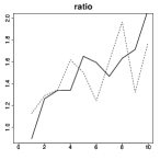
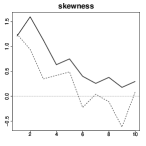
Figure 1: Left: Ratio of variance to mean for 10 different binning of both treatment, solid line, and placebo group, dashed line. Right: skewness for 10 different binning of both treatment, solid line, and placebo group, dashed line.

Clearly, for both groups and all the 10 bin-lengths we observe overdispersion, Figure 1, which is interpreted as existence of a random effect. However, the plot dose not show any meaningful difference in the amount of overdispersion between the two groups. Nevertheless, there seems to be a difference in the skewness structure between the two groups; the treatment group has positive skewness for all 10 bin lengths, while the placebo group has negative skewness for $\gamma=6,7,8,9$. As illustrated in the simulation study in Section 3, when there is left-skewness in the random effect the local mixture method returns smaller bias and standard deviation since it is flexible enough to adjust for it. Therefore, we expect discrepancy in coefficient estimates between the two methods for placebo group, while they are almost similar for the treatment group.

6 Appendix

Proof 4

(Lemma 2) For $k=4$ (without lose of generality), $\Lambda_{b}(\vartheta)$ can be parametrized using the solution set of equations $q(y)=0$, $q^{\prime}(y)=0$, as functions of $\lambda_{2}$, $\lambda_{3}$ and $\lambda_{4}$ for all $y>0$, which retain the locus of the intersecting line for any two consecutive supporting planes (Do Carmo 1976 ch.2). Direct calculation shows that $\Lambda_{b}(\vartheta)$ can be obtained by the following smooth mapping,

$$\mathcal{C}:(0,\infty)\times U\rightarrow R^{3},\hskip 28.45274pt(y,\lambda_{2})=\left[\lambda_{2},\lambda_{3}(y,\lambda_{2}),\lambda_{4}(y,\lambda_{2})\right]$$

where, $U\subset R$ is an open interval and

$$\lambda_{3}(y,\lambda_{2})=\frac{2(y^{3}-5y^{2}+8y)\lambda_{2}+4y-12}{y^{2}(y^{2}-6y+12)},\,\,\,\,\,\,\,\,\lambda_{4}(y,\lambda_{2})=\frac{(y^{3}-4y^{2}+6y)\lambda_{2}+3y-6}{y^{3}(y^{2}-6y+12)}$$

Therefore, the implicit function theorem (Rudin, 1976, p.224) implies that $\Lambda_{b}(\vartheta)$ is a smooth manifold.

In general, the boundary of parameter space of local mixture models may not be smooth manifolds; hence, in those situations either the possible singularity points must be characterized or other optimization approaches must be applied for finding maximum on boundary.

Algorithm Description

To clarify the technical background and convergence proof of the algorithm, the following paragraphs are in order. For convenience we present the local mixture term in (6) by $l_{\vartheta}(\lambda)$.
In step (2a), $t_{j}$ is tangent to $\Lambda_{b}(\vartheta)$ at $\lambda^{(j-1)}=\lambda^{\star}$ and can be obtained as follows. If we collect the quartic $q(y)$ in (8) with respect to $\lambda_{2}^{\star}$, $\lambda_{3}^{\star}$ and $\lambda_{4}^{\star}$, we obtain the supporting plane with the normal vector $(y^{\star 2}-2y^{\star},\,-y^{\star 3}+3y^{\star 2},\,y^{\star 4}-4y^{\star 3})$, where $y^{\star}$ is the real multiple root of $q(y)$.

In step (2b), $\Pi_{j}=I-N_{j}N_{j}^{T}$ presents the matrix of orthogonal projection onto tangent plane $t_{j}$, with respect to Euclidean inner product, in which $I$ is the identity matrix. Therefore, for $g_{j}$ and $H_{j}$ the gradient vector and hessian matrix of $l_{\vartheta}(\lambda)$ at $\lambda^{(j-1)}$, the first and second covariant derivatives are $\Pi_{j}g_{j}$ and $\Pi_{j}H_{j}$, respectively.

Step (2c), describes the so called exponential -also called retraction- mapping $R:T\Lambda_{b}(\vartheta)\rightarrow\Lambda_{b}(\vartheta)$, where $T\Lambda_{b}(\vartheta)$ represents the tangent bundle of $\Lambda_{b}(\vartheta)$, the disjoint union of $t_{j}$’s (See Shub 1986). Let $R_{j}$ be the restriction of $R$ to $t_{j}$, then $R_{j}$ is a one-to-one mapping that maps the vector $(\Pi_{j}H_{j}^{-1})(\Pi_{j}g_{j})\in t_{j}$ to a curve between $\lambda^{(j-1)}$ and $R_{j}(\lambda^{(j)})$ on $\Lambda_{b}(\vartheta)$ and holds the following assumptions,

• $R_{j}$ is defined in an open interval $U_{r_{j}}(0_{j})\in t_{j}$, about $0_{j}$ of radius $r_{j}>0$, where $0_{j}$ is the representation of $\lambda^{(j-1)}$ in $t_{j}$.

• $R_{j}(\dot{\lambda})=\lambda$ if and only if $\dot{\lambda}=0_{j}$.

• $R$ is smooth and $DR_{j}(0_{j})=id_{t_{j}}$, since $R_{j}(\lambda^{(j-1)})=\lambda^{(j-1)}$.

Figure 2: Schematic visualization of the algorithm steps

Proof 5

(Theorem 2) Consider the following two cases,
(I) $\hat{\lambda}\in\Lambda(\vartheta)$
Since $l_{\vartheta}(\lambda)$, for any fixed $\vartheta$, is strictly concave and satisfy the second-order sufficient conditions, then step (1) of the algorithm converges to the unique global maximum $\hat{\lambda}$ in quadratic order, for any initial point $\lambda^{(0)}$ inside the interior of $\Lambda(\vartheta)$ (see Nocedal & Wright 2006 p.45).
(II) $\hat{\lambda}\notin\Lambda(\vartheta)$
Since $\Lambda(\vartheta)$ is closed and convex in a finite dimensional vector space, there is a unique $\hat{\lambda}_{b}\in\Lambda(\vartheta)$ with minimum distance from $\hat{\lambda}$, and consequently $l_{\vartheta}(\hat{\lambda}_{b})\geq l_{\vartheta}(\lambda)$ for all $\lambda\in\Lambda(\vartheta)$, since $l_{\vartheta}(\lambda)$ is strictly concave. Moreover, the vector $\hat{\lambda}_{b}\hat{\lambda}$ is orthogonal to the supporting plane $t_{b}$, tangent to $\Lambda(\vartheta)$ at $\hat{\lambda}_{b}$; hence, $(\Pi_{b}g_{b})$ is a zero vector in the tangent vector space $t_{b}$.
In addition, according to Lemma 2, $\Lambda_{b}(\vartheta)$, is a locally smooth manifold embedded in $R^{k-1}$. According to notations in Shub (1986), step 2 can be presented by the following mapping

$$\mathcal{S} : \Lambda_{b}(\vartheta)\rightarrow\Lambda_{b}(\vartheta)$$

$$\lambda^{(j-1)} \rightarrow R_{j}\left(\lambda^{(j-1)}\,,\,(\Pi_{j}H_{j}^{-1})(\Pi_{j}g_{j})\right)$$ (12)

where, by condition (3), $\mathcal{S}$ is smooth. Also, if $(\Pi_{j}H_{j}^{-1})$ exists then by conditions (1) and (2), the fixed points of $\mathcal{S}$ (i.e, $\mathcal{S}(\lambda)=\lambda$) are the zero’s of the covariant gradient, and at fixed points the derivative of $\mathcal{S}$ vanishes.

References

- Abbring and Van Den Berg [2007] J. H. Abbring and G. J. Van Den Berg. The unobserved hetreogeneity distribution in duration analysis. Biometrika, 94(1):87–99, 2007.
- Anaya-Izquierdo and Marriott [2007] K. Anaya-Izquierdo and P. Marriott. Local mixture models of exponential families. Bernoulli, 13:623–640, 2007.
- Berger [1987] M. Berger. Geometry I. Springer, 1987.
- Breslow [1972] N. Breslow. Contribution to the discuassion on the paper of cox (1972). Biom, 34:216–217, 1972.
- Clayton [1978] D. G. Clayton. A model for association in bivariate life tables and its application in epidemiological studies of familial tendency in chronic disease incidence. Biometrika, 65(1):141–151, 1978.
- Clayton and Cuzick [1985] D. G. Clayton and J. Cuzick. Multivariate generalizations of the proportional hazard model. Journal of the Royal Statistical Society A, 148(2):82–117, 1985.
- Cox [1972] D. R. Cox. Regression models and life-tables. Journal of the Royal Statistical Society B, 34:187–200, 1972.
- Eleber and Ridder [1982] C. Eleber and G. Ridder. True and spurious duration dependence: The identifiability of the proportional hazard model. Review of Economic Studies, 49:403–409, 1982.
- Fuchs et al. [1994] H. J. Fuchs, B. D. S., D. H. Christiansen, E. M. Morris, M. L. Nash, B. W. Ramsey, B. J. Rosenstein, A. L. Smith, and M. E. Wohl. Effect of aerosolized recombinant human dnase on exacerbations of respiratory symptoms on pulmonary function in paitients with cystic fibrosis. New Eng. J. Med, 331:637–643, 1994.
- Gorfine et al. [2006] M. Gorfine, D. M. Zucher, and L. Hsu. Prospective survival analysis with general semiparametric shared frialty model: A pseudo full likelihood approach. Biometrika Trust, 93(3):735–741, 2006.
- Horowitz [1999] J. L. Horowitz. Semiparametric estimation of a proportional hazard model with unobserved hetrogeneity. Econometrica, 67(5):1001–1028, 1999.
- Horowitz [2010] J. L. Horowitz. Semiparametric and Nonparametric Methods in Econometrics. Springer, 2010.
- Hougaard [1984] P. Hougaard. Life table methods for heterogeneous populations: Distributions describing the heterogeneity. Biometrika, 71(1):75–83, 1984.
- Hougaard [1986] P. Hougaard. Survival models for heterogeneus population derived from stable distributions. Biometrika, 73(2):387–396, 1986.
- Hsu et al. [2004] L. Hsu, L. Chen, M. Gorfine, and K. Malone. Semiparametric estimation of marginal hazard function from case-control family studies. Biometrics, 60:936–944, 2004.
- Hu et al. [2011] T. Hu, B. Nan, X. Lin, and J. M. Robbins. Time-dependent cross ratio estimation for bivariate failure times. Biometrika, 98(2):341–354, 2011.
- Johansen [1983] S. Johansen. An extenssion of cox’s regression model. International Statistical Review, 51:258–262, 1983.
- Jorgensen [1997] B. Jorgensen. The Theory of Dispersion Models. London: Chapman and Hull, 1997.
- Klein [1992] J. P. Klein. Semiparametric estimation of random effects using cox model based on the em algorithm. Biometrics, 48:795–806, 1992.
- Lawless [1981] J. F. Lawless. Statistical Models and Methods for Lifetime Data. Wiley, 1981.
- Marriott [2002] P. Marriott. On the local geometry of mixture models. Biometrika, 89:77–93, 2002.
- Martinussen et al. [2011] T. Martinussen, T. H. Scheike, and D. M. Zucker. The aalen additive gamma frailty hazard model. Biometrika, 98(4):831–843, 2011.
- Nan et al. [2006] B. Nan, X. Lin, L. D. Lisabeth, and S. Harlow. Piecewise constant cross ratio estimation for association of age at a marker event age at a menopause. Journal of the American Statistical Association, 101:65–77, 2006.
- Nielsen et al. [1992] G. G. Nielsen, R. D. Gill, P. K. Anderson, and T. I. A. Sorensen. A counting process approach to maximum likelihood estimation in frailty models. Scandinavian Journal of Statistics, 19(1):25–43, 1992.
- Oakes [1982] D. Oakes. A model for association in bivariate survival data. Journal of the Royal Statistical Society B, 44(3):414–422, 1982.
- Rudin [1976] W. Rudin. Principles of Mathematical Analysis. New York: McGraw-Hill, 3rd edition, 1976.
- Shub [1986] M. Shub. Some remarks on dynamical systems and numerical analysis. Proc. VII ELAM (L. Lara-Carrero and J. Lewowicz, eds.), Equinoccio, U. Simon Bolivar, Caracas, 69-92, pages 69–92, 1986.
- Small [2010] C. G. Small. Expansions and Asymptotics for Statistics. Chapman and Hall, 2010.
- Ulrich and Watson [1994] G. Ulrich and L. T. Watson. Positivity conditions for quartic polynomials. AIAM J. Sci. Comput., 15:528–544, 1994.
- Vaupel et al. [1979] J. W. Vaupel, K. G. Manton, and E. Stallard. The impact of heterogeneity in individual frailty on the dynamics of mortality. Demography, 16:539–454, 1979.
- Zeng et al. [2009] D. Zeng, Q. Chen, and J. Ibrahim. Gamma frailty transformation models for multivariate survival times. Biometrika, 96(2):277–291, 2009.