Spreading of correlations and Loschmidt echo after quantum quenches of a Bose gas in the Aubry-André potential

Abstract

We study the spreading of density-density correlations and the Loschmidt echo, after different sudden quenches in an interacting one dimensional Bose gas on a lattice, also in the presence of a superimposed aperiodic potential. We use a time dependent Bogoliubov approach to calculate the evolution of the correlation functions and employ the linked cluster expansion to derive the Loschmidt echo.

I Introduction

The study of the behavior of many-body quantum systems driven out-of-equilibrium has attracted a lot of attention in the last few years. In particular theoretical and experimental interest on how fast the correlations can spread in quantum many-body systems kollath2008 ; cheneau2012 ; ronzheimer2013 ; vidmar2013 ; carleo ; jurcevic2014 has been renewed after the work by Calabrese and Cardy calabrese2006 . They showed that, for critical theories the maximum velocity of the spreading of correlations is given by the group velocity in the final gapless system. Actually the existence of a maximal velocity lieb1972 known as the Lieb-Robinson bound, has been shown to exist theoretically in several interacting many-body systems, due to short range interactions which may reduce the propagation of information making its spreading speed finite.

In this work we study the spreading of density-density correlations following sudden quantum quenches in a system of bosons held in a bichromatic lattice. The case of bosons placed on a lattice is a paradigm of interacting many-body systems, which can be experimentally reproduced by means of ultracold atomic gases and described theoretically by the well known Bose-Hubbard model. Beyond the maximum velocity, one can wonder how correlations evolve at later times. It has been shown natu2013 that, for bosons on a periodic lattice, density-density correlations spread diffusively after an initial ballistic motion. One issue worth being addressed is therefore related to the effects of a modulated potential on such behaviors. We were inspired by a recent experimental work modugno2013 in which transport of bosons in a bichromatic optical lattice was studied.

Besides the correlation spreading there are other quantities, useful to characterize the dynamics of a quantum system and its approach to equilibrium, if any. The Loschmidt echo is perhaps one of the most used tools to investigate the dynamics of a quantum system following a sudden quench. Physically, it is the probability for the system to return to its initial state after a certain time. It is particularly sensitive to both the initial state and the spectrum of the system after the sudden quench and it thus reveals critical behaviors of the system sindona2013 ; schiro . Moreover it has been shown that the echo is related to the work distribution, which in turn is a very useful quantity when thermodynamical properties of a closed quantum system are considered sindona2014 .

In this paper we show how to calculate the evolution of correlation functions in interacting bosonic systems by means of a time dependent Bogoliubov approach mora2003 , and derive non-perturbatively the Loschmidt echo, by means of linked cluster expansion mattuck .

II Model and method

We consider a system of interacting bosons in a 1D lattice with on-site interaction. In the single band approximation, this system is described by the the Bose-Hubbard Hamiltonian

$${\hat{\cal H}}=-\frac{J}{2}\sum\limits_{\langle i,j\rangle}^{L}\hat{b}_{i}^{\dagger}\hat{b}_{j}+\sum\limits_{i}^{L}V_{i}\,\hat{b}_{i}^{\dagger}\hat{b}_{i}+\frac{U}{2}\sum\limits_{i}^{L}\hat{n}_{i}(\hat{n}_{i}-1),$$ (1)

where $\hat{b}^{\dagger}_{i}$ and $\hat{b}_{i}$ are bosonic creation and annihilation operators defined on the lattice sites, $V_{i}$ are the on-site energies, $J$ the hopping parameter between nearest neighbor sites, $U$ the on-site boson-boson interaction, $\hat{n}_{i}=\hat{b}^{\dagger}_{i}\hat{b}_{i}$ the number operator and $L$ the number of sites. In what follows we will consider a modulation of the on-site potential of the Aubry-André type (also known as Harper model),

$$V_{i}=\lambda\cos\left(2\pi\tau\,i\right),$$ (2)

where we choose $\tau=(\sqrt{5}+1)/2$, the golden ratio. In the non-interacting case, $U=0$, it has been proven rigorously jitomirskaya1999 that the above system shows a metal-insulator like transition at $\lambda=\lambda_{c}=1$ (here and in what follows we assume $J=1$). For $\lambda>\lambda_{c}$ all eigenstates are exponentially localized, while in the case $\lambda<\lambda_{c}$ are all delocalised. This peculiarity leads, in the presence of weak interaction, to the existence of a superfluid state even for finite values of $\lambda$, in contrast to uncorrelated disorder, which, even in the presence of a small amount, is more effective to bring the system to a Bose glass phase. This behavior has been confirmed in several works where the phase diagram of the model described by Eq. (1) has been derived roux2008 ; roscilde2008 ; deng2008 , showing that, for $\lambda<1$ and moderate interaction, the system is in a superfluid phase.

This allow us to safely address the case of weakly interacting bosons at zero temperature by means of the time-dependent Bogoliubov approach even at finite values of $\lambda$. In the high filling limit, weak boson-boson interaction plays an important rôle, not because of particle interaction but because of the eventually large number of particles on single sites dutta2011 . We assume, therefore, $U\left\langle\hat{n}_{i}\right\rangle$ not too large, and consider small quantum fluctuations.

In this limit we can separate the bosonic operator into a spatially varing classical part (mean field) and a quantum part (quantum fluctuations)

$$\hat{b}_{i}=\sqrt{N_{0}}\,\phi_{i}+\hat{c}_{i}$$ (3)

with $N_{0}$ the (macroscopic) number of particles occupying the state $\phi_{i}$.

Within gaussian approximation in the fluctations, we get the following effective Bogoliubov Hamiltonian

$$\hat{H} = \sum_{i}\left(V_{i}-\mu+2g|\phi_{i}|^{2}\right)\hat{c}^{\dagger}_{i}\hat{c}_{i}-\frac{J}{2}\sum_{\langle i,j\rangle}\hat{c}^{\dagger}_{i}\hat{c}_{j}$$

$$+\frac{g}{2}\sum_{i}(\phi_{i}^{2}\,\hat{c}_{i}^{\dagger}\hat{c}_{i}^{\dagger}+\phi^{*2}_{i}\,\hat{c}_{i}\hat{c}_{i}),$$

where $g=UN_{0}$. The macroscopically occupied state $\phi_{i}$ and the chemical potential $\mu$ satisfy the stationary Gross-Pitaevskii equation

$$-\frac{J}{2}(\phi_{i+1}+\phi_{i-1})+g|\phi_{i}|^{2}\phi_{i}+V_{i}\phi_{i}=\mu\phi_{i}.$$ (5)

The Hamiltonian in Eq.(II) can be diagonalized by means of the Bogoliubov transformations (see Sec. III). We solved Eq. (5) and diagonalized Eq.(II) iteratively by fixing the total number of particles in a system of $L=100$ sites to be $N=500$, setting $N_{0}=N-N_{ex}$ where $N_{ex}$ is the number of particles in the excited states. Usually after five iterations the solution converges and we checked that $N_{ex}\ll N_{0}$ for all ranges of parameters we have used, in accordance with the assumtion of small fluctuations.

In Fig.1 we plot the band spectrum of the Bogoliubov modes as a function of $\lambda$ at fixed $U$, and as a function of $U$ at fixed $\lambda$. One can notice that the effect of the interaction is not only that of closing the sub-bands, as expected, but also making the inter-band localized state to migrate from the higher energy sub-band to the lower energy one.

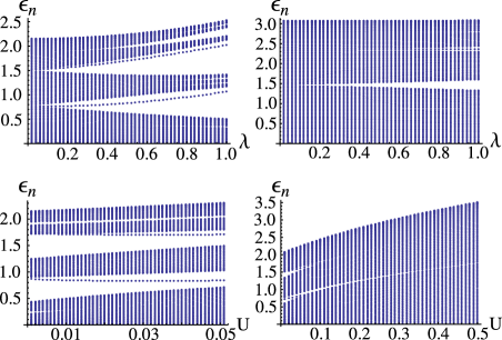
Figure 1: Bogoliubov bands (top row) as functions of $\lambda$ at (left) $U=0.03$ and (right) $U=0.3$ and (bottom row) as functions of $U$, at $\lambda=0.5$, for small (left) and large (right) values of $U$.

III Quantum quenches

In this section we present the formalism used to look at the dynamics of the system following a sudden quench in the Hamiltonian. In the following sections we will consider quenches resulting from a sudden change in i) $U$ at fixed $\lambda$, ii) $\lambda$ at fixed $U$.

It is worth mentioning that with the Bogoliubov approach the system is closed but not isolated. In fact the system described by the effective Hamiltonian in Eq. (II) does not conserve the total number of quasi-particles if a parameter is changed. This is due to the fact that also the chemical potential changes and the system can exchange particles with the superfluid part. Therefore we are dealing with a system, which can exchange particles with a reservoir.

Let us call $H_{0}$ the initial Hamiltonian at time $t=0$, described by Eq. (II) with initial parameters ($U=U_{0}$, $V_{i}=V_{0i}$, and, from Eq. (5), $\mu=\mu_{0}$, $N_{0}=N_{00}$) while $H$ in Eq. (II) is the Hamiltonian after the quench. Both $H_{0}$ and $H$ can be diagonalized by the following canonical Bogoliubov transformations

$$\hat{c}_{i} = \sum_{n}u_{i,n}\,\hat{\alpha}_{n}-v^{*}_{i,n}\,\hat{\alpha}^{\dagger}_{n}\,,$$ (6)

$$\hat{c}_{i} = \sum_{n}\omega_{i,n}\,\hat{\beta}_{n}-w^{*}_{i,n}\,\hat{\beta}^{\dagger}_{n}\,,$$ (7)

with conditions $\sum_{i}(u_{in}u^{*}_{im}-v_{in}v^{*}_{im})=\sum_{i}(\omega_{in}\omega^{*}_{im}-w_{in}w^{*}_{im})=\delta_{nm}$ , ensuring that the above transformation are indeed canonical, so that by Eqs. (6), (7) we get

$$\hat{H}_{0}=\sum_{n}\epsilon^{0}_{n}\,\hat{\alpha}^{\dagger}_{n}\hat{\alpha}_{n}\,,$$ (8)

$$\hat{H}=\sum_{n}\epsilon_{n}\,\hat{\beta}^{\dagger}_{n}\hat{\beta}_{n}\,,$$ (9)

where $n$ labels the eigenmodes. Thus we can write the operators $\hat{\beta}_{n}$ of the diagonalized final Hamiltonian in terms of the Bogoliubov operators $\alpha_{n}$ of the initial Hamiltonian

$$\left(\begin{array}[]{c}\hat{\beta}_{n}\\ \hat{\beta}_{n}^{\dagger}\end{array}\right)=\sum_{m}\left(\begin{array}[]{cc}\Lambda_{nm}&\Omega^{*}_{nm}\\ \Omega_{nm}&\Lambda^{*}_{nm}\end{array}\right)\left(\begin{array}[]{c}\hat{\alpha}_{m}\\ \hat{\alpha}_{m}^{\dagger}\end{array}\right)$$ (10)

where

$$\Lambda_{nm}=\sum_{i}\omega^{*}_{i,n}u_{i,m}-w^{*}_{i,n}v_{i,m}$$ (11)

$$\Omega_{nm}=\sum_{i}w_{i,n}u_{i,m}-\omega_{i,n}v_{i,m}$$ (12)

When $H=H_{0}$, $\Lambda_{nm}=\delta_{nm}$ and $\Omega_{nm}=0$ due to the conditions on the coefficients of the transformations. The initial state $|\psi(0)\rangle$ is chosen to be the vacuum state of $H_{0}$, namely $\alpha_{n}|\psi_{0}\rangle=0$ $\forall n$, while the evolution of the original operators in the Heisenberg picture, is given by

$$\hat{c}_{i}(t)=\sum_{n}\omega_{i,n}\,\hat{\beta}_{n}e^{-i\epsilon_{n}t}-w^{*}_{i,n}\,\hat{\beta}^{\dagger}_{n}e^{i\epsilon_{n}t},$$ (13)

where $\epsilon_{n}$ are the Bogoliubov energies of the final Hamiltonian $H$. Thus we are able to calculate the time evolution of all correlation functions, within the gaussian approximation, on the ground state of $H_{0}$, by means of Eq. (10).

IV Correlation functions

In what follows we will consider the normal ordered density-density correlators between different sites at different times,

$${\cal G}_{i,j}(t,t^{\prime})=\langle:{\hat{n}}_{i}(t)\hat{n}_{j}(t^{\prime}):\rangle-\langle\hat{n}_{i}(t)\rangle\langle\hat{n}_{j}(t^{\prime})\rangle\,.$$ (14)

At the leading order in the fluctuations, neglecting variation of $\phi$ for small quenches and using Eq. (3), we have

$${\cal G}_{i,j}(t,t^{\prime})\simeq 2N_{0}\textrm{Re}\left[\phi_{i}\phi_{j}^{*}\,\langle\hat{c}_{i}^{\dagger}(t)\hat{c}_{j}(t^{\prime})\rangle+\phi^{*}_{i}\phi^{*}_{j}\,\langle\hat{c}_{i}(t)\hat{c}_{j}(t^{\prime})\rangle\right].$$ (15)

Therefore, we need to calculate only $\langle\hat{c}_{i}^{\dagger}(t)\hat{c}_{j}(t^{\prime})\rangle$ and $\langle c_{i}(t)c_{j}(t^{\prime})\rangle$. From Eq. (13) and its conjugate counterpart, and Eq. (10), and exploiting the fact that the initial state is the vacuum state of the $\hat{\alpha}$’s, we get

$$\langle\hat{c}_{i}^{\dagger}(t)\hat{c}_{j}(t^{\prime})\rangle=\sum_{n,\ell,m}\left\{\omega^{*}_{i,n}\omega_{j,\ell}\,\Omega_{nm}\Omega^{*}_{\ell m}\,e^{i(\epsilon_{n}t-\epsilon_{\ell}t^{\prime})}+w_{i,n}w^{*}_{j,\ell}\,\Lambda_{nm}\Lambda^{*}_{\ell m}\,e^{-i(\epsilon_{n}t-\epsilon_{\ell}t^{\prime})}\right.$$

$$\left.-\omega^{*}_{i,n}w^{*}_{j,\ell}\,\Omega_{nm}\Lambda^{*}_{\ell m}\,e^{i(\epsilon_{n}t+\epsilon_{\ell}t^{\prime})}-w_{i,n}\omega_{j,\ell}\,\Lambda_{nm}\Omega^{*}_{\ell m}\,e^{-i(\epsilon_{n}t+\epsilon_{\ell}t^{\prime})}\right\}$$ (16)

$$\langle\hat{c}_{i}(t)\hat{c}_{j}(t^{\prime})\rangle=\sum_{n,\ell,m}\left\{\omega_{i,n}\omega_{j,\ell}\,\Lambda_{nm}\Omega^{*}_{\ell m}\,e^{-i(\epsilon_{n}t+\epsilon_{\ell}t^{\prime})}+w^{*}_{i,n}w^{*}_{j,\ell}\,\Omega_{nm}\Lambda^{*}_{\ell m}\,e^{i(\epsilon_{n}t+\epsilon_{\ell}t^{\prime})}\right.$$

$$\left.-\omega_{i,n}w^{*}_{j,\ell}\,\Lambda_{nm}\Lambda^{*}_{\ell m}\,e^{-i(\epsilon_{n}t-\epsilon_{\ell}t^{\prime})}-w^{*}_{i,n}\omega_{j,\ell}\,\Omega_{nm}\Omega^{*}_{\ell m}\,e^{i(\epsilon_{n}t-\epsilon_{\ell}t^{\prime})}\right\}.$$ (17)

In what follows we will look at the following function

$$\Delta{\cal G}_{i}(t,t^{\prime})={\cal G}_{i,i_{0}}(t,t^{\prime})-{\cal G}_{i,i_{0}}(0,0)$$ (18)

with $i_{0}$ a fixed point of the lattice, which in the following will be chosen to be $i_{0}=L/2$. In particular we will look at $\Delta{\cal G}_{i}(t,0)$, which gives us information on the propagation of the effect of a perturbation acting at $i_{0}$ at time $t=0$ after some time $t$ at a point $i$.

The density-density correlation function at different times, in Fourier space, is also called dynamical structure factor. This quantity has been calculated for the Lieb-Liniger model calabrese2006_2 , namely for a 1D Bose gas in the continuum. As also reported in Ref. calabrese2006_2 , the dynamical structure factor and, therefore, the density-density correlation function at different times, is experimentally accessible either by Fourier sampling of time of flight images duan2006 or through Bragg spectroscopy ketterle1999 . More recently a direct, real-time and nondestructive measurement of the dynamic structure factor has been realized for a Bose gas to reveal a structural phase transition esslinger .

IV.1 Periodic case $(\lambda=0)$

We start the discussion about the behavior of the density-density correlation functions by first looking at the homogeneous case. In this case only a quench in the boson-boson interaction $U$ can be performed.

In Fig. 2 we show the propagation of density-density correlations. We can clearly see that the fastest signal is ballistic and that the speed of propagation increases by increasing $U_{0}$ together with its amplitude (see Fig. 3), while the slower diffusive part is very intense for small $U_{0}$ and almost disappear for large $U_{0}$.
The velocity of the fast signals is, therefore, constant and given by the maximum value of the group velocity in the final system calabrese2006 , which, from the single particle dispersion $\varepsilon_{k}=J(1-\cos k)$ and the Bogoliubov spectrum $\epsilon_{k}=\sqrt{\varepsilon_{k}(\varepsilon_{k}+2\nu U)}$, is given by

$$v=\frac{J(\varepsilon_{k_{m}}+\nu U)\sin k_{m}}{\epsilon_{k_{m}}}$$ (19)

where $\nu$ is the filling and

$$k_{m}=2\arccos\sqrt{\frac{3}{4}+\frac{3\nu U}{J}-\frac{\sqrt{J^{2}(J^{2}+6J\nu U+5\nu^{2}U^{2})}}{4J^{2}}}.$$ (20)

For $U\simeq 0.4$, $\nu\simeq 5$ and $J=1$, the speed given by the Eq. (19) is $v\approx 1.4$, in agreement with the speed of the propagation shown in the last pannel of Fig. 2, with same parameters. For relatively small $\nu U$, we can approximate $k_{m}\simeq\pi/2$ and, therefore, the speed is simply given by

$$v\simeq\frac{J(J+\nu U)}{\sqrt{J(J+2\nu U)}}.$$ (21)

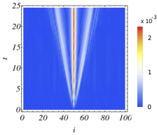
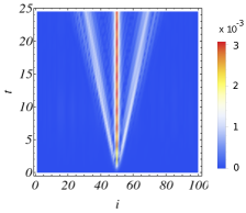
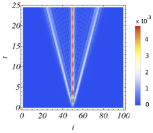
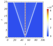
Figure 2: (Color online) $\Delta{\cal G}_{i}(t,0)$, Eq. (18), after quenches from $U_{0}=0.025$ (top left), $0.05$ (top right), $0.15$ (bottom left), $0.35$ (bottom right), to $U=U_{0}+0.05$, as a function of the distance $i$ and time $t$ at $\lambda=0$. Here and in all the figures, $t$ is in unit of $J^{-1}$ and $i$ in unit of the lattice spacing.

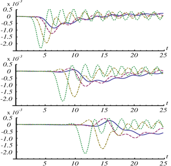
Figure 3: (Color online) $\Delta{\cal G}_{i}(t,0)$ for $i-i_{0}=5,10,15,20$, after a quench from $U_{0}=0.025$ (solid line), $U_{0}=0.05$ (dashed line), $U_{0}=0.15$ (dot-dashed line), $U_{0}=0.35$ (dotted line), as a function of time $t$. $U-U_{0}=0.05$ for all quenches.

IV.2 Quench in $U$

Let us first consider the quench in the boson-boson interaction $U$. For this case we can compare the results in the absence of a modulation of the on-site energies ($\lambda=0$) with those obtained at finite $\lambda$.

In Figs. 4 and 5 we plot $\delta{\cal G}_{i}(t,0)$ after a small quench in a weakly interacting system, from $U_{0}=0.025$ to $U=0.03$, for different values of $\lambda$. As shown in those plots, the switching on of the Aubry-André potential is the fate of the fast signals which otherwise would travel ballistically at constant velocity given by Eq. (19). The spreading is then overall diffusive, although made of rare, sharp and asymmetric timelike signals (see the pattern made of stipes in time, shown in Fig. 4). Increasing $\lambda$ the signals become sparser and sparser, and eventually disappear approaching the Bose glass phase.

In Fig. 6, we plot $\delta{\cal G}_{i}(t,0)$ for a larger quench in a stronger interacting system, namely from $U_{0}=0.25$ to $U=0.3$ for different values of $\lambda$. In this case we notice that the maximum speed at which the signals travel, does not depend upon $\lambda$. This can be seen by looking at the wings of the signal which have the same width for all values of $\lambda$ and is clearly visible in the plots of Fig. 7 by looking at the position of the first peak for different values of $\lambda$ and different distances. On the other hand, as $\lambda$ increases the signal goes from a purely ballistic dynamics, namely a localized packet traveling at a constant velocity (see the $\lambda=0$ case) to a more broadened propagation inside the ”light-cone”.

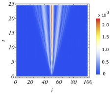
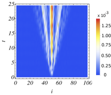
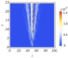
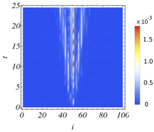
Figure 4: (Color online) $\Delta{\cal G}_{i}(t,0)$, Eq. (18), after a quench from $U_{0}=0.025$ to $U=0.03$, as a function of the distance $i$ and time $t$, for different values of $\lambda$: $\lambda=0$ (top left), $0.3$ (top right), $0.6$ (bottom left), $0.9$ (bottom right).

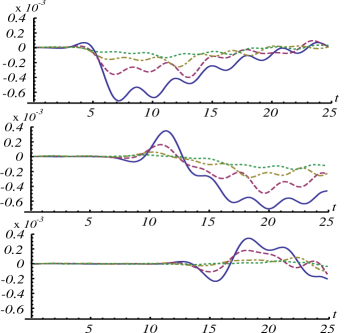
Figure 5: (Color online) $\Delta{\cal G}_{i}(t,0)$ for $i-i_{0}=5,10,15,20$, after a quench from $U_{0}=0.025$ to $U=0.03$ as a function of time $t$ for $\lambda=0$ (solid line), $\lambda=0.3$ (dashed line), $\lambda=0.6$ (dot-dashed line), $\lambda=0.9$ (dotted line).

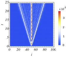
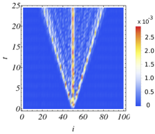
Figure 6: (Color online) $\Delta{\cal G}_{i}(t,0)$, Eq. (18), after a quench from $U_{0}=0.25$ to $U=0.3$, as a function of the distance $i$ and time $t$, for different values of $\lambda$: (from top left to bottom right) $\lambda=0,0.3,0.6,0.9$.

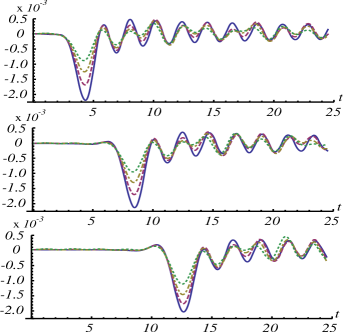
Figure 7: (Color online) $\Delta{\cal G}_{i}(t,0)$ for $i-i_{0}=5,10,15,20$, after a quench from $U_{0}=0.25$ to $U=0.3$ as a function of time $t$ for $\lambda=0$ (solid line), $\lambda=0.3$ (dashed line), $\lambda=0.6$ (dot-dashed line), $\lambda=0.9$ (dotted line).

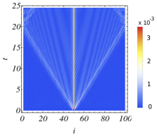
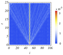
Figure 8: (Color online) $\Delta{\cal G}_{i}(t,t)$, Eq. (18), after a quench from $U_{0}=0.25$ to $U=0.3$, as a function of the distance $i$ and time $t$, for $\lambda=0$ (left), and $\lambda=0.6$ (right).

Finally, let us look at the equal time density-density correlation function $\Delta{\cal G}_{i}(t,t)$. As shown in Fig. 8, where we plot $\Delta{\cal G}_{i}(t,t)$ after a quench in $U$ for two different values of $\lambda$, the spreading, whose intensity is much weaker than that of $\Delta{\cal G}_{i}(t,0)$, describes a cone with a velocity just twice larger than that of the corresponding $\Delta{\cal G}_{i}(t,0)$, in particular, in the periodic case ($\lambda=0$), the velocity is $2v$ with $v$ given by Eq. (19). Analogously to the different time correlators, this velocity is not affected by the aperiodic potential.

IV.3 Quench in $\lambda$

We now consider the case of quenches in the potential strength $\lambda$ at fixed boson-boson interaction $U$. In Fig. 9 we show the function $\delta{\cal G}_{i}(t,0)$ for a quench from $\lambda_{0}=0.5$ to $\lambda=0.55$, for different values of the boson-boson interaction, namely $U=0.1,0.2,0.3,0.4$. In this case we can clearly see an increase in the speed propagation of the signal as $U$ increases (widening of the outermost wings), better visible in Fig. 10 where the signal appears at early times as $U$ is increased for a given distance from $i_{0}$. This is in agreement with the fact that, in the homogeneous system, an increase in the boson-boson interaction would lead to an increase of the group velocity. For large $U$, therefore, the Aubry-André potential becomes marginal even if the dynamics is generated by a sudden quench of $\lambda$. Moreover, increasing $U$ we notice that the slower diffusive signals become weaker and weaker exhibiting a crossover to an almost pure ballistic expansion.

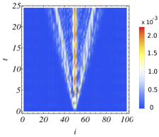
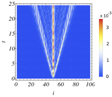
Figure 9: (Color online) $\Delta{\cal G}_{i}(t,0)$, after a quench from $\lambda_{0}=0.5$ to $\lambda=0.55$, for different values of $U$: (from top left to bottom right) $U=0.1,0.2,0.3,0.4$.

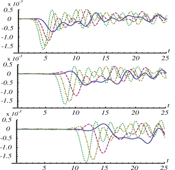
Figure 10: (Color online) $\Delta{\cal G}_{i}(t,0)$ for $i-i_{0}=5,10,15,20$, after a quench from $\lambda_{0}=0.5$ to $\lambda=0.55$ as a function of time $t$ for $U=0.1$ (solid line), $U=0.2$ (dashed line), $U=0.3$ (dot-dashed line), $U=0.4$ (dotted line).

V Momentum distribution

In this section we look at the (time dependent) momentum distribution defined as the Fourier transform of the one-body density matrix

$$n(k,t) = \frac{1}{L}\sum\limits_{i,j}e^{-\imath k(i-j)}\left\langle\hat{b}^{\dagger}_{i}(t)\hat{b}_{j}(t)\right\rangle$$

$$= n_{0}(k)+n_{ex}(k,t)$$

with $\hat{b}$ given by Eq. (3), $n_{0}(k)=\frac{N_{0}^{2}}{L}\sum_{i,j}e^{-\imath k(i-j)}\phi_{i}^{*}\phi_{j}$, is the mean field contribution, and $n_{ex}(k,t)=\frac{1}{L}\sum\limits_{i,j}e^{-\imath k(i-j)}\langle\hat{c}^{\dagger}_{i}(t)\hat{c}_{j}(t)\rangle$ the fluctuation contribution.

In Fig. 11 we plot the momentum distribution $n(k,t)$ at two different times, at $t=0$ and at later time after a sudden change of the boson-boson interaction $U$. Three peaks are clearly visible at $k=0,\pm 2\pi(1-\tau^{-1})$ due to the presence of the modulation of the potential, in agreement with DMRG (density matrix renormalization group) calculations reported in Refs. roux2008 ; deng2008 , where it was shown that peaks appear at $k=\pm 2\pi(1-r)$, if the on-site potential has the functional form $\cos(2\pi ri)$. In our case $r=\tau=1+\tau^{-1}$ and thus $\cos(2\pi\tau i)=\cos(2\pi i/\tau)$. The quantum quench in $U$ weakly modifies the profile of the momentum distribution, at least in the time scale considered, inducing a small modulation due to quantum fluctuations. This result suggests that one has to rather focus on the density-density correlations for better detecting the effects of quench dynamics.

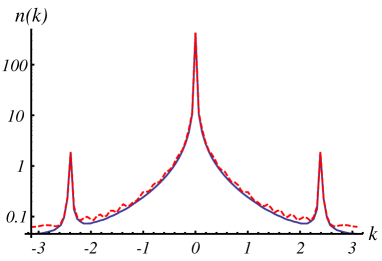
Figure 11: (Color online) Momentum distribution $n(k,t)$, Eq. (V) with $L=100$, at $t=0$ (solid blue line) and at $t=12.5$ (dashed red line) after a quench from $U_{0}=0.25$ to $U=0.3$.

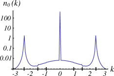
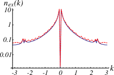
Figure 12: (Color online) Mean field ($n_{0}$) and fluctuation ($n_{ex}$) contributions to the momentum distribution for $\lambda=0.6$, at $t=0$ (solid blue line) and at $t=12.5$ (dashed red line) after a sudden quench from $U_{0}=0.25$ to $U=0.3$. Large ticks on the $k$-axis of the plot for $n_{0}(k)$, highlight features at $k=\pm 2\pi(1-\tau^{-1})/\tau^{\ell}$ with $\ell=0,1,2$.

Looking carefully at the mean field term, $n_{0}(k)$ (see Fig. 12), we notice other peculiar features due to the scaling propeties of the Aubry-André potential, at positions $k=\pm 2\pi(1-\tau^{-1})/\tau^{\ell}$ with $\ell=0,1,2$, while the contribution due to fluctuations $n_{ex}(k,t)$ (Fig. 12, plot on the right) exhibits dips at $k=0,\pm 2\pi(1-\tau^{-1})$ at any time. This ensures that the time dependent Bogoliubov approach is consistent with the assumption that the mean field dynamics can be neglected on the time scales considered.

VI Loschmidt echo

In this section we calculate the vacuum persistence amplitude following a sudden quench, defined as

$$\nu(t)=\left\langle e^{i\hat{H}_{0}t}\,e^{-i\hat{H}t}\right\rangle,$$ (23)

where the average is over the initial state, $|\psi(0)\rangle$, namely the vacuum state for $\hat{\alpha}_{n}$, $\hat{\alpha}_{n}|\psi(0)\rangle=0$. It is, therefore, convenient to define

$$\delta{\hat{H}}=\hat{H}-\hat{H}_{0}$$ (24)

so that we can rewrite Eq. (23)

$$\nu(t)=\left\langle{\mathcal{T}}e^{-i\int_{0}^{t}d\tau\,\delta\hat{H}(\tau)}\right\rangle$$ (25)

$$\phantom{\nu(t}=\sum_{n=0}^{\infty}\frac{(-i)^{n}}{n!}\int_{0}^{t}d\tau_{1}...\int_{0}^{t}d\tau_{n}\,\langle{\mathcal{T}}[\delta\hat{H}(\tau_{1})...\delta\hat{H}(\tau_{n})]\rangle$$

where $\delta\hat{H}(\tau)=e^{i\hat{H}_{0}\tau}\,\delta\hat{H}\,e^{-i\hat{H}_{0}\tau}$, in the interaction picture with respect to the Hamiltonian $\hat{H}_{0}=\sum_{n}\epsilon^{0}_{n}\hat{\alpha}^{\dagger}_{n}\hat{\alpha}_{n}$.
For simplicity, calling $h_{ij}=(V_{i}-\mu+2g|\phi_{i}|^{2})\delta_{ij}-J\delta_{j,i\pm 1}$ and $\Delta_{i}=g\phi_{i}^{2}/2$, we rewrite Eq. (II) as

$$\hat{H}=\sum_{i,j}h_{ij}\,\hat{c}^{\dagger}_{i}\hat{c}_{j}+\sum_{i}(\Delta_{i}\,\hat{c}^{\dagger}_{i}\hat{c}^{\dagger}_{i}+\Delta^{*}_{i}\,\hat{c}_{i}\hat{c}_{i}).$$ (26)

Analogously, we can rewrite $H_{0}$ with $h^{0}_{ij}$ and $\Delta^{0}_{i}$, and $\delta\hat{H}$ with $\delta h_{ij}=h_{ij}-h^{0}_{ij}$ and $\delta\Delta_{i}=\Delta_{i}-\Delta^{0}_{i}$. By applying the Bogoliubov transformation in Eq.(6), one can write $\delta\hat{H}$ in terms of the initial Bogoliubov operators, $\alpha_{n}$, which in the interaction picture can be written as

$$\delta\hat{H}(\tau)=E_{0}+\sum_{n,\ell}A_{n\ell}\,e^{i(\epsilon^{0}_{n}-\epsilon^{0}_{\ell})\tau}\hat{\alpha}^{\dagger}_{n}\hat{\alpha}_{\ell}$$ (27)

$$\phantom{\delta H}+\sum_{n,\ell}\left(B_{n\ell}\,e^{-i(\epsilon^{0}_{n}+\epsilon^{0}_{\ell})\tau}\hat{\alpha}_{n}\hat{\alpha}_{\ell}+B^{*}_{n\ell}\,e^{i(\epsilon^{0}_{n}+\epsilon^{0}_{\ell})\tau}\hat{\alpha}^{\dagger}_{\ell}\hat{\alpha}^{\dagger}_{n}\right)$$

where the constant term

$$E_{0}=\sum_{\ell}\Big{(}\sum_{i,j}\delta h_{ij}\,v_{i,\ell}v^{*}_{j,\ell}-2\sum_{i}\textrm{Re}\left[\delta\Delta_{i}\,u^{*}_{i,\ell}v_{i,\ell}\right]\Big{)}$$

is just a phase shift in Eq. (25), while

$$A_{n\ell}=\sum_{i,j}\delta h_{ij}(u^{*}_{i,n}u_{j,\ell}+v_{i,\ell}v^{*}_{j,n})$$

$$\phantom{A_{n\ell}}-2\sum_{i}\textrm{Re}\left[\delta\Delta_{i}(u^{*}_{i,n}v_{i,\ell}+v_{i,\ell}u^{*}_{i,n})\right]$$ (28)

$$B_{n\ell}=\sum_{i}(\delta\Delta_{i}v_{i,n}v_{i,\ell}+\delta\Delta^{*}_{i}u_{i,n}u_{i,\ell})-\sum_{i,j}\delta h_{ij}v_{i,n}u_{j,\ell}$$

Notice that, since $\delta h_{ij}=\delta h_{ji}$, then $A_{n\ell}=A^{*}_{\ell_{n}}$, as should be in order for $\delta\hat{H}$ to be hermitian. Moreover, in Eq. (27), because of commutation relations, only the symmetric part of $B_{n\ell}$, namely $(B_{n\ell}+B_{\ell n})/2$, plays a role, analogously for $B^{*}_{n\ell}$.
Now, exploiting the linked cluster expansion theorem, we get

$$\ln{\nu(t)}={-iE_{0}t}+{\sum_{q=1}^{\infty}{\cal C}_{q}(t)}$$ (30)

where ${\cal C}_{q}=(-i)^{q}\int_{0}^{t}d\tau_{1}...\int_{0}^{\tau_{q-1}}d\tau_{q}\,\langle\delta^{\prime}\hat{H}(\tau_{1})...\delta^{\prime}\hat{H}(\tau_{q})\rangle_{c}$ is the sum of all connected diagrams of the $q$-th order in the perturbation parameters $\delta h_{ij}$, $\delta\Delta_{i}$ and where $\delta^{\prime}\hat{H}=\delta\hat{H}-E_{0}$. In what follows we will consider diagrams up to third order. After time integration, we get (${\cal C}_{1}(t)=0$)

$${\cal C}_{2}(t) = 2i\sum_{n,\ell}\frac{|B_{n\ell}|^{2}}{(\epsilon^{0}_{n}+\epsilon^{0}_{\ell})}\;t-2\sum_{n,\ell}\frac{|B_{n\ell}|^{2}}{(\epsilon^{0}_{n}+\epsilon^{0}_{\ell})^{2}}\left(1-e^{-i(\epsilon^{0}_{n}+\epsilon^{0}_{\ell})t}\right)$$ (31)

$${\cal C}_{3}(t) = -4i\sum_{n,\ell,m}\frac{B^{*}_{n\ell}\,B_{\ell m}\,A_{mn}}{(\epsilon^{0}_{n}+\epsilon^{0}_{\ell})(\epsilon^{0}_{\ell}+\epsilon^{0}_{m})}\;t+4\sum_{n,\ell,m}\frac{B^{*}_{n\ell}\,B_{\ell m}\,A_{mn}}{\epsilon^{0}_{n}-\epsilon^{0}_{m}}\left[\frac{1-e^{-i(\epsilon^{0}_{\ell}+\epsilon^{0}_{m})t}}{(\epsilon^{0}_{\ell}+\epsilon^{0}_{m})^{2}}-\frac{1-e^{-i(\epsilon^{0}_{n}+\epsilon^{0}_{\ell})t}}{(\epsilon^{0}_{n}+\epsilon^{0}_{\ell})^{2}}\right]$$ (32)

One can easly show, by the properties os the coefficients $A_{n\ell}$ and $B_{n,\ell}$, that the first terms of Eqs. (31), (32) are purely imaginary. However, without loss of generality, since $u_{i,n}$, $v_{i,n}$ and $\phi_{i}$ can be chosen to be real, then also $A_{n\ell}$ and $B_{n\ell}$ can be real.

In the following we will look at the behavior of the Loschmidt echo defined as

$${\cal L}(t)=|\nu(t)|^{2}=e^{\sum_{q}2\textrm{Re}[{\cal C}_{q}(t)]}$$ (33)

after a quantum quench in the interaction ($U$) or in the potential ($\lambda$) parameters.

VI.1 Periodic case, $\lambda=0$

As a reference, let us first consider the homogeneous case ($\lambda=0$). In this case only an interacting quench can be made ($\delta U\neq 0$), and, keeping for simplicity only the first non-vanishing contribution, Eq. (31), dominant for small $\delta U$, we get

$$\textrm{Re}[{\cal C}_{2}]=-\frac{\delta g^{2}}{4}\sum_{k}\left(\frac{\sin(\sqrt{\varepsilon_{k}(\varepsilon_{k}+2U_{0}\nu_{0})}\,t)}{\varepsilon_{k}+2\nu_{0}U_{0}}\right)^{2}$$ (34)

where $\varepsilon_{k}=J(1-\cos k)$ is the single particle dispersion, $\nu_{0}=N_{00}/L$ the condensate density at $t=0$, $U_{0}$ the initial value of the interaction parameter, and finally $\delta g=g-g_{0}=UN_{0}-U_{0}N_{00}$. A rought evaluation of Eq. (34) can be obtained expanding $\varepsilon_{k}\simeq Jk^{2}/2$, so that $\textrm{Re}[{\cal C}_{2}]\simeq-\frac{\delta g^{2}}{8\pi}\frac{\pi(1-e^{-4U_{0}\nu_{0}t}(1+4U_{0}\nu_{0}t)}{16\sqrt{J}(U_{0}\nu_{0})^{3/2}}$, finding that, for large time, the Loschmidt echo saturates at the value

$${\cal L}\left(t\gtrsim(U_{0}\nu_{0})^{-1}\right)\propto\exp\left[-\frac{\delta g^{2}}{(U_{0}\nu_{0})^{{3}/{2}}}\right]$$ (35)

At later time further corrections may play a role and the third order diagrams need to be included.

VI.2 Quenches in $U$

In the case of a quench in $U$ the echo shows a quadratic decay at short times and an exponential decay on longer time scales approaching a stationary value approximatelly given by Eq. (35), which however does not correspond to the overlap between the initial vacuum state and the one of the final Hamiltonian. Oscillations around this stationary value are induced by the bandwidth. At finite $\lambda$, the presence of additional sub-bands, as shown in Fig. 1, induces further low frequencies in the echo. From Fig. 13, we see that also for moderately large quench amplitudes the echo is always close to one, meaning that a quench in $U$ does not make the system to fully explore the phase space and the system stays close to its initial state.
The effect of $\lambda$ is to make the system more chaotic further reducing the overlap between the initial and the time evolved state for large $U$. Remarkably, at low $U$, the Loschmidt echo, at $t>(U\nu)^{-1}$, increases as $\lambda$ is increased, as shown in the first plot of Fig. 13.

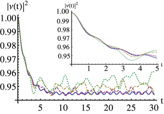
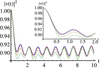
Figure 13: (Color online) ${\cal L}(t)$, after a quench (top) from $U_{0}=0.05$ to $U=0.06$ and (bottom) from $U_{0}=0.25$ to $U=0.3$, for different values of $\lambda=\lambda_{0}$: $\lambda=0$ (solid line), $\lambda=0.3$ (dashed line), $\lambda=0.6$ (dot-dashed line), $\lambda=0.9$ (dotted line). In the insets the short time dynamics of the echo showing the characteristic quadratic decay at short times.

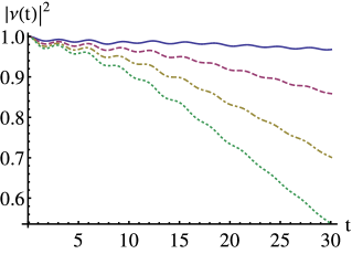
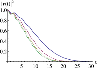
Figure 14: (Color online) ${\cal L}(t)$, after a quench from $\lambda_{0}=0.5$ to $\lambda=0.55$, for different values of $U=U_{0}$, (top) for small values: $U=0.01$ (solid line), $U=0.02$ (dashed line), $U=0.03$ (dot-dashed line), $U=0.04$ (dotted line), and (bottom) for larger values: $U=0.1$ (solid line), $U=0.2$ (dashed line), $U=0.3$ (dot-dashed line), $U=0.4$ (dotted line).

VI.3 Quenches in $\lambda$

When quenching in $\lambda$ the situation is quite different. As we can see from Fig. 14 the echo decays to zero, with an almost gaussian tail, in a finite time and the characteristic time decay is set by $U$, namely the larger is $U$, the faster is the decay of the echo. This means that a quench in $\lambda$ has the effect of making the system to explore a very large portion of the accessible phase space, contrary to the case of the quench in $U$ where the system remains trapped in a smaller region of the same space.

VII Conclusions

In this paper we report on the study of quantum quenches in a system of ultracold bosons in a bichromatic optical lattice, described by a Bose-Hubbard model, in the Bogoliubov approximation. In particular we looked at the dynamics of the density-density correlation functions at different times and at the Loschmidt echo following a quench in the on-site boson-boson interaction $U$ or in the strength of the optical lattice $\lambda$. We found that when quenching in $U$ at low $\lambda$ the spreading of correlation functions is ballistic with a speed, which is independent of $\lambda$. By increasing $\lambda$ the signal becomes more noisy due to the fragmentation of the energy spectrum. Moreover, as shown by the Loschimdt echo, after a quench in $U$, the final state has a large overlap with the initial one, which, unexpectedly, can be even larger increasing $\lambda$.
On the other hand, when quenching in $\lambda$ at different $U$ the spreading of correlations goes from a disordered to a ballistic motion as $U$ increases. Moreover, the system seems to end in a state, which is completely orthogonal to the initial one as witnessed by the echo.

- (1) A.M. Läuchli, C. Kollath, Spreading of correlations and entanglement after a quench in the one-dimensional Bose-Hubbard model, J. Stat. Mech.: Theory Exp. (2008) P05018
- (2) M. Cheneau, P. Barmettler, D. Poletti, M. Endres, P. Schauß, T. Fukuhara, C. Gross, I. Bloch, C. Kollath, S. Kuhr, Light-cone-like spreading of correlations in a quantum many-body system, Nature 481, 484 (2012)
- (3) J.P. Ronzheimer, M. Schreiber, S. Braun, S.S. Hodgman, S. Langer, I.P. McCulloch, F. Heidrich-Meisner, I. Bloch, U. Schneider, Expansion dynamics of interacting bosons in homogeneous lattices in one and two dimensions, Phys. Rev. Lett. 110, 205301 (2013)
- (4) L. Vidmar, S. Langer, I. P. McCulloch, U. Schneider, U. Schollwöck, and F. Heidrich-Meisner, Sudden expansion of Mott insulators in one dimension, Phys. Rev. B 88, 235117 (2013)
- (5) G. Carleo, F. Becca, L. Sanchez-Palencia, S. Sorella, M. Fabrizio, Light-cone effect and supersonic correlations in one- and two-dimensional bosonic superfluids, Phys. Rev. A 89, 031602(R) (2014)
- (6) P. Jurcevic, B.P. Lanyon, P. Hauke, C. Hempel, P. Zoller, R. Blatt, C.F. Roos, Quasiparticle engineering and entanglement propagation in a quantum many-body system, Nature 511, 202 (2014)
- (7) P. Calabrese, J. Cardy, Time dependence of correlation functions following a quantum quench, Phys. Rev. Lett. 96, 136801 (2006)
- (8) E.H. Lieb, D.W. Robinson, The finite group velocity of quantum spin systems, Commun. Math. Phys. 28, 251–257 (1972)
- (9) S.S. Natu, E. J. Mueller, Dynamics of correlations in a dilute Bose gas following an interaction quench, Phys. Rev. A87, 053607 (2013)
- (10) L.Tanzi, E. Lucioni, S. Chaudhuri, L. Gori, A. Kumar, C. D’Errico, M. Inguscio, G. Modugno, Transport of a Bose Gas in 1D Disordered Lattices at the Fluid-Insulator Transition, Phys. Rev. Lett. 111 ,115301 (2013)
- (11) A. Sindona, J. Goold, N. Lo Gullo, S. Lorenzo, F. Plastina, Orthogonality catastrophe and decoherence in a trapped-Fermion environment Phys. Rev. Lett. 111, 165303 (2013)
- (12) M. Schiró, A. Mitra, Transient orthogonality catastrophe in a time-dependent nonequilibrium environment, Phys. Rev. Lett. 112, 246401 (2014)
- (13) A. Sindona, J. Goold, N. Lo Gullo, F. Plastina Statistics of the work distribution for a quenched Fermi gas, New Journal of Physics 16, 045013 (2014)
- (14) C. Mora and Y. Castin Extension of Bogoliubov theory to quasicondensates, Phys. Rev. A67, 053615 (2003)
- (15) R.D. Mattuck, A guide to Feynman diagrams in the many-body problem, New York, McGraw-Hill, (1976)
- (16) S.Y. Jitomirskaya, Metal-insulator transition for the almost Mathieu operator,Ann. of Math. 150, 1159 (1999)
- (17) G. Roux, T. Barthel, I.P. McCulloch, C. Kollath, U. Schollwöck, and T. Giamarchi, Quasiperiodic Bose-Hubbard model and localization in one-dimensional cold atomic gases, Phys. Rev. A78, 023628 (2008)
- (18) T. Roscilde, Bosons in one-dimensional incommensurate superlattices, Phys. Rev. A77, 063605 (2008)
- (19) X. Deng, R. Citro, A. Minguzzi, E. Orignac, Phase diagram and momentum distribution of an interacting Bose gas in a bichromatic lattice, Phys. Rev. A78, 013625 (2008)
- (20) O. Dutta, A. Eckardt, P. Hauke, B. Malomed and M. Lewenstein, Bose–Hubbard model with occupation-dependent parameters, New J. Phys. 13, 023019 (2011)
- (21) J.-S. Caux and P. Calabrese, Dynamical density-density correlations in the one-dimensional Bose gas, Phys. Rev. A74, 031605(R) (2006)
- (22) L.-M. Duan, Detecting Correlation Functions of Ultracold Atoms through Fourier Sampling of Time-of-Flight Images, Phys. Rev. Lett. 96, 103201 (2006)
- (23) J. Stenger, S. Inouye, A. P. Chikkatur, D. M. Stamper-Kurn, D. E. Pritchard, and W. Ketterle, Bragg Spectroscopy of a Bose-Einstein Condensate, Phys. Rev. Lett. 82, 4569 (1999)
- (24) R. Landig, F. Brennecke, R. Mottl, T. Donner, T. Esslinger, Measuring the dynamic structure factor of a quantum gas undergoing a structural phase transition, Nat. Commun. 6, 7046 (2015)