Massive Yang-Mills for Vector and Axial-Vector Spectral Functions at Finite Temperature

Abstract

The hadronic mechanism which leads to chiral symmetry restoration is explored in the context of the $\rho\pi a_{1}$ system using Massive Yang-Mills, a hadronic effective theory which governs their microscopic interactions. In this approach, vector and axial-vector mesons are implemented as gauge bosons of a local chiral gauge group. We have previously shown that this model can describe the experimentally measured vector and axial-vector spectral functions in vacuum. Here, we carry the analysis to finite temperatures by evaluating medium effects in a pion gas and calculating thermal spectral functions. We find that the spectral peaks in both channels broaden along with a noticeable downward mass shift in the $a_{1}$ spectral peak and negligible movement of the $\rho$ peak. The approach toward spectral function degeneracy is accompanied by a reduction of chiral order parameters, i.e., the pion decay constant and scalar condensate. Our findings suggest a mechanism where the chiral mass splitting induced in vacuum is burned off. We explore this mechanism and identify future investigations which can further test it.

I Introduction

Chiral symmetry is a basic symmetry of quantum chromodynamics (QCD), the theory of the strong nuclear force. This symmetry is spontaneously broken in the vacuum via the formation of quark condensates. At higher temperatures, the symmetry is restored as the condensates melt passing through a pseudo-critical region Borsanyi:2010bp ; Bazavov:2011nk around $T_{\rm pc}\simeq$ 160 MeV. This behavior is imprinted on the hadronic spectra when heating up the vacuum. Despite these well-established properties of QCD, the hadronic mechanism leading to chiral restoration is not fully understood to date.

The only in-medium hadronic spectral function which is experimentally accessible is that of the light vector mesons, dominated by the $\rho$, which can be probed via low-mass dilepton spectra in heavy-ion collisions Porter:1997rc ; Adamova:2006nu ; Arnaldi:2008fw ; Agakishiev:2011vf ; Geurts:2012rv . Theory calculations reveal that the experimental data are compatible with a $\rho$ melting scenario whereby the spectral peak broadens without a significant shift in its mass, see, e.g., Refs. Rapp:2009yu ; Rapp:2013nxa . It has been conjectured that this broadening is an indication of chiral symmetry restoration based on QCD and chiral sum rules Hohler:2013eba . However, for a definitive assertion of restoration, the in-medium spectral function of the chiral partner of the $\rho$, namely the light axial-vector meson $a_{1}$, needs to be calculated to test spectral degeneracy. This spectral function is difficult to measure experimentally. Thus one is led to study the $\rho\pi a_{1}$ system theoretically to establish chiral restoration.

Recent sum rule analyses indicate that the experimental dilepton measurements are consistent with an approach towards restoration and spectral degeneracy between the vector ($V$) and axial-vector ($AV$) channels Hohler:2013eba . This degeneracy is imprinted on the $a_{1}$ spectral function by a mass shift toward the $\rho$ mass, accompanied by spectral broadening. This analysis suggests a possible mechanism for restoration in the hadronic spectrum. However, other analyses suggest that the sum rules can be satisfied in medium without a mass shift or a need to approach spectral degeneracy Ayala:2014rka . Therefore, it is in order to explore the mechanism from a microscopic perspective.

A theoretically appealing construction is to implement the $\rho$ and $a_{1}$ as the gauge bosons of a local chiral gauge group Yang:1954ek . This combines chiral effective theories, which have had considerable success in describing pion driven low-energy properties of QCD Gasser:1983yg , with the general field theoretical concept of gauge symmetries. This has been realized in two formalisms, Massive Yang-Mills (MYM) Gomm:1984at and Hidden Local Symmetry (HLS) Bando:1987br ; Harada:2003jx , which have been shown to be on-shell equivalent.

Early applications of MYM successfully describe the tree level masses and decays of the $\rho$ and $a_{1}$ mesons Gomm:1984at ; Song:1993ae ; Ko:1994en . These studies were extended to finite temperatures Song:1993af ; Song:1993ipa ; Pisarski:1995xu revealing a reduction of the $a_{1}$ mass along with an increase in the $\rho$ mass. However, these calculations do not survive the scrutiny of a loop calculation needed to determine the vacuum spectral functions which have been experimentally measured with high precision through $\tau$ leptons decaying into multi-pion states Barate:1998uf ; Ackerstaff:1998yj . An in-medium mass reduction in the $a_{1}$ spectral function is also compatible with the HLS framework Harada:2008hj , though a satisfactory description of vacuum spectral functions has not yet been demonstrated either.

The complications in describing the vacuum spectral functions with MYM and HLS triggered investigations which abandon the local implementation of the gauge group in favor of a global one Urban:2001ru ; Wagner:2008gz ; Parganlija:2010fz . These models have also been extended to include temperature effects; using a loop expansion, a broadening of the $\rho$ spectral peak without a mass shift was found in Ref. Urban:2001uv , whereas Ref. Struber:2007bm , using a 2-particle irreducible truncation scheme for the in-medium masses, found a slightly increasing $\rho$-mass to degenerate with a dropping $a_{1}$-mass above the critical temperature.

In a recent work, we have re-evaluated MYM as an effective theory to describe the light-meson chiral properties, and were able to overcome the initial difficulties associated with the vacuum spectral functions Hohler:2013ena . This was made possible by two critical ingredients: a fully dressed $\rho$ propagator in the calculation of the $a_{1}$ self-energy, and the inclusion of a chirally invariant continuum. In the present paper, motivated by this development and the theoretical appeal of MYM, we implement this approach in a finite-temperature pion gas, examining the medium modifications of the spectral functions to deduce information on the hadronic mechanism of chiral restoration.

Our paper is organized as follows. In Sec. II, we briefly introduce MYM. In Sec. III, we recall our strategy of implementing a broad $\rho$ spectral function into the vacuum MYM framework, and extend our earlier work to the linear $\sigma$ model and with further applications to vacuum observables. In Sec. IV, the in-medium $\rho$ and $a_{1}$ spectral functions are calculated including polarization and 3-momentum dependencies. In Sec. V, we illustrate and quantify the progression towards chiral symmetry restoration by computing the pion decay constant and the scalar condensate. In Sec. VI, we conduct a more general discussion on the mechanism of chiral restoration in light of our and related works on the subject, and identify promising directions of future work. We summarize and conclude in Sec. VII.

II The Massive Yang-Mills Lagrangian

In the MYM approach Gomm:1984at ; Song:1993ae , the chiral pion Lagrangian is locally gauged under the symmetry group $SU(2)_{L}\times SU(2)_{R}$. In this paper, we will explore both the linear and non-linear realization of this symmetry. The explicit form of the Lagrangian, including the higher derivative “non-minimal” terms, is given by

$$\begin{split}\mathcal{L}_{\rm MYM}&=\frac{\tilde{f}_{\pi}^{2}}{8}({\rm Tr}[D_{\mu}U^{\dagger}D^{\mu}U]+\tilde{m}_{\pi}^{2}{\rm Tr}[U+U^{\dagger}-2])\\ &-\frac{1}{2}{\rm Tr}[F_{L}^{2}+F_{R}^{2}]+m_{0}^{2}{\rm Tr}[A_{L}^{2}+A_{R}^{2}]\\ &-i\xi\ {\rm Tr}[D_{\mu}UD_{\nu}U^{\dagger}F_{L}+D_{\mu}U^{\dagger}D_{\nu}UF_{R}]\\ &+\gamma\ {\rm Tr}[F_{L}UF_{R}U^{\dagger}]\ .\end{split}$$ (1)

Implicit in this Lagrangian is a derivative expansion in the chiral pion fields but not in the gauge fields.

In the non-linear realization, the pion fields are generated by expanding the ansatz for the field $U$=$\exp\left[{2\pi i}/{F_{\pi}}\right]$ with $\pi=\pi^{a}\tau_{a}/\sqrt{2}$, where $\tau_{a}$ are the Pauli matrices – the generators of the symmetry group. The gauge coupling, $g$, figures in the Lagrangian through the covariant derivative, $D_{\mu}U$=$\partial_{\mu}U-ig(A_{L\mu}U-UA_{R\mu})$ where $A_{L/R}^{\mu}=\left(A_{L/R}^{\mu}\right)^{a}\tau_{a}/\sqrt{2}$. Vector and axial-vector combinations of the gauge fields are defined as

$$V_{\mu}=A_{L\mu}+A_{R\mu}\,,\quad A_{\mu}=A_{L\mu}-A_{R\mu}\ .$$ (2)

The last term in the Lagrangian induces a contribution to the gauge fields’ kinetic terms which can be absorbed by a field redefinition. Thus the physical $\rho$ and $a_{1}$ fields, $\rho_{\mu}$ and $a_{\mu}$, are defined as

$$\rho_{\mu}=\kappa_{V}^{-1}V_{\mu} a_{\mu}=\kappa_{A}^{-1}A_{\mu}$$ (3)

$${\rm with}\quad\kappa_{V}=(1-\gamma)^{-1/2} \kappa_{A}=(1+\gamma)^{-1/2}\ .$$

Mass terms, $m_{0}$ and $\tilde{m}_{\pi}$, for the physical fields are added which explicitly break the gauge and chiral symmetries. The unphysical $a_{\mu}\partial^{\mu}\pi$ coupling is removed by the shift $a_{\mu}\rightarrow a_{\mu}+\alpha Z_{\pi}\partial_{\mu}\pi$. The physical pion mass and decay constant can then be defined in terms of the Lagrangian couplings and the pion field renormalization, $Z_{\pi}$, as $M_{\pi}$=$Z_{\pi}\tilde{m}_{\pi}$=139.6 MeV and $F_{\pi}$=$\tilde{f_{\pi}}/Z_{\pi}$=131 MeV with

$$Z_{\pi}=\left(1-\frac{g_{\rho\pi\pi}^{2}F_{\pi}^{2}}{2M_{\rho}^{2}}\right)^{-1/2}.$$ (4)

The coupling to external electro-weak (EW) fields is accomplished by gauging the fields under the same symmetry group as the mesons, with the coupling constant fixed by the charge of the pion. This includes the addition of kinetic terms for the EW fields, new chirally and gauge invariant interactions between the EW and meson fields of a form similar to the Kroll, Lee, and Zumino coupling Kroll:1967it , i.e., $F_{L}^{\rm EW}F_{L}$, as well as interactions of the form of the non-minimal terms. All couplings associated with the external fields are dictated by gauge symmetry and related to the parameters in Eq. (1). In the end, the Lagrangian contains four parameters: the gauge coupling, $g$, the bare gauge boson mass, $m_{0}$, and two non-minimal couplings, $\gamma$ and $\xi$. These can be traded for the phenomenologically more pertinent parameters of the single- and triple-derivative $\rho\pi\pi$ couplings, $g_{\rho\pi\pi}$ and $g_{\rho\pi\pi}^{(3)}$, and the bare masses of the $\rho$ and $a_{1}$, $M_{\rho}$ and $M_{a_{1}}$. Expressing them in terms of the Lagrangian parameters leads to

$$g_{\rho\pi\pi}=\frac{1}{\sqrt{2}}g\kappa_{V}; g_{\rho\pi\pi}^{(3)}=\frac{4\kappa_{V}\xi}{\sqrt{2}F_{\pi}^{2}Z_{\pi}^{4}}-\frac{F_{\pi}^{2}g^{3}}{8\sqrt{2}m_{0}^{4}\kappa_{V}}$$

$$M_{\rho}^{2}=\kappa_{V}^{2}m_{0}^{2}; M_{a_{1}}^{2}=\kappa_{A}^{2}(m_{0}^{2}+\frac{1}{2}g_{\rho\pi\pi}^{2}F_{\pi}^{2}Z_{\pi}^{2})\ ,$$ (5)

which highlights the chiral splitting between the bare $\rho$ and $a_{1}$ masses through the spontaneous symmetry breaking represented by the pion decay constant. The interaction vertices of the physical fields are then obtained by expanding the Lagrangian; they are spelled out in Appendix A.

In the linear realization of the pion Lagrangian, an explicit $\sigma$ field is kept which may be viewed as resumming a set of $\pi\pi$ $s$-wave interactions of the non-linear formalism. This is achieved by evaluating the Lagrangian in Eq. (1) with the linear ansatz $U=\sqrt{2}/F_{\pi}(\sigma\mathbb{I}/Z_{\pi}+\sqrt{2}i\pi)$, where $\mathbb{I}$ is the unit matrix in isospin space. Two additional Lagrangian terms must be added to describe the scalar potential

$$\mathcal{L}=-\frac{\tilde{f_{\pi}^{2}}}{8}\left(\mu^{2}{\rm Tr}\left[U^{\dagger}U\right]+\frac{\lambda}{4}\tilde{f_{\pi}^{2}}\,{\rm Tr}\left[\left(U^{\dagger}U\right)^{2}\right]\right)\,.$$ (6)

The potential parameters $\mu$ and $\lambda$ are fixed by the vacuum pion and sigma masses, inducing a spontaneous breaking of the gauge symmetry resulting in a vacuum expectation value (VEV) for the $\sigma$ field, $\sigma_{0}$, related to the chiral condensate. The physical $\sigma$ field is then redefined relative to the vacuum, $\sigma\rightarrow\sigma+\sigma_{0}$. The VEV of the $\sigma$ field is related to the pion decay constant as $\sigma_{0}=F_{\pi}Z_{\pi}/\sqrt{2}$.

While the physical $\rho$ and $a_{1}$ fields are defined in the same manner as in the non-linear case, the field renormalizations and their masses (as well as the pion renormalization, $Z_{\pi}$) can be expressed in terms of the VEV $\sigma_{0}$ as

$$\kappa_{V,A} = (1\mp\frac{2\gamma\sigma_{0}^{2}}{F_{\pi}^{2}Z_{\pi}^{2}})^{-1/2}$$

$$Z_{\pi}^{2} = 1+\frac{g_{\rho\pi\pi}^{2}\sigma_{0}^{2}}{M_{\rho}^{2}}$$

$$g_{\rho\pi\pi} = g\kappa_{V}/\sqrt{2}$$ (7)

$$g_{\rho\pi\pi}^{(3)} = \frac{4\kappa_{V}\xi}{\sqrt{2}F_{\pi}^{2}Z_{\pi}^{4}}-\frac{\sigma_{0}^{2}g^{3}}{4\sqrt{2}m_{0}^{4}Z_{\pi}^{2}\kappa_{V}}$$

$$M_{\rho}^{2} = \kappa_{V}^{2}m_{0}^{2}$$

$$M_{a_{1}}^{2} = \kappa_{A}^{2}\left(m_{0}^{2}+g_{\rho\pi\pi}^{2}\sigma_{0}^{2}\right)\ .$$

Evaluating these expressions with the vacuum value for $\sigma_{0}$ results in the same expressions as in the non-linear case. The relevant vertices of the linear realization are also given in Appendix A.

III Vacuum spectral functions in the vector and axial-vector channels

We are interested in the $V$ and $AV$ spectral functions as probed by an external EW current. The correlators of these currents are defined as

$$\Pi_{V,A}^{\mu\nu}(q^{2})=-i\int d^{4}x\ e^{ixq}\left<T\vec{J}_{V,A}^{\mu}(x)\vec{J}_{V,A}^{\nu}(0)\right>\ .$$ (8)

In each channel, there are two independent polarization functions, for the 4D-transverse and 4D-longitudinal components. The correlators can be expressed in terms of these functions as

$$\Pi_{V,A}^{\mu\nu}(q^{2})=\Pi_{V,A}^{T}(q^{2})\left(-g^{\mu\nu}+\frac{q^{\mu}q^{\nu}}{q^{2}}\right)+\Pi_{V,A}^{L}(q^{2})\frac{q^{\mu}q^{\nu}}{q^{2}}\,.$$ (9)

Because of gauge invariance, $\Pi_{V}^{L}=0$, while $\Pi_{A}^{L}$ plays an important role in verifying that the chiral properties inherent in the Lagrangian are maintained once loops are included.

The current-current correlators with external EW fields can be constructed from the sum of a direct term and one which transitions through a resonant meson. For example, for the $V$ channel, the correlator is comprised of the photon self-energy, $\Sigma_{\gamma}^{T}$, plus a term which converts a photon into a $\rho$ meson, $\Gamma_{V}^{T}$, propagates the $\rho$, and finally converts the $\rho$ back into a photon. This, and the processes for the $AV$ channels, are depicted diagrammatically in Fig. 1. For the transverse mode, the correlators are expressed as

$$\Pi_{V/A}^{T}(p^{2})=\Sigma_{\gamma/W}^{T}(p^{2})+\left(\Gamma_{V/A}^{T}(p^{2})\right)^{2}\!\!D_{V/A}^{T}(p^{2}),$$ (10)

with the propagators given by

$$D_{V,A}^{T}\left(p^{2}\right)=\left(p^{2}-M_{\rho,a_{1}}^{2}-\Sigma_{\rho,a_{1}}^{T}\left(p^{2}\right)\right)^{-1}.$$ (11)

The transition functions, $\Gamma_{V/A}^{T}$, describe the conversion of a photon/W boson into a $\rho$/$a_{1}$ meson and are comprised of a contact contribution and a self-energy given by

$$\Gamma_{V}^{T}(p^{2}) = \frac{p^{2}}{g_{\rho\pi\pi}}+\Sigma_{\gamma\rho}(p^{2}),$$ (12)

$$\Gamma_{A}^{T}(p^{2}) = \frac{p^{2}}{g_{\rho\pi\pi}}-\frac{g_{\rho\pi\pi}F_{\pi}^{2}M_{a_{1}}Z_{\pi}}{2M_{\rho}}+\Sigma_{Wa_{1}}^{T}(p^{2}).$$ (13)

Figure 1: Schematic depiction of the contributions to the EW current-current correlators. The bold lines in the center indicate fully resummed propagators.

The $V$ and $AV$ transverse spectral functions are defined in terms of the 4D-transverse current-current correlator associated with the external EW fields, $\rho_{V/A}^{T}\equiv-{\rm Im}\Pi_{V/A}^{T}/\pi$. Due to the gauging procedure, the EW self-energies can be expressed in terms of the mesonic self-energies as

$$\begin{split}\Sigma_{\gamma}^{T}=\frac{1}{g_{\rho\pi\pi}^{2}}\Sigma_{\rho}^{T}(p^{2}),&\quad\Sigma_{\gamma\rho}=-\frac{1}{g_{\rho\pi\pi}}\Sigma_{\rho}^{T}(p^{2}),\\ \Sigma_{W}^{T}=\frac{M_{\rho}^{2}Z_{\pi}^{2}}{g_{\rho\pi\pi}^{2}M_{a_{1}}^{2}}\Sigma_{a_{1}}^{T}(p^{2}),&\quad\Sigma_{Wa_{1}}=-\frac{M_{\rho}Z_{\pi}}{g_{\rho\pi\pi}M_{a_{1}}}\Sigma_{a_{1}}^{T}(p^{2})\,.\end{split}$$ (14)

Using these relations, the spectral functions emerge in a form suggestive of (axial-) vector meson dominance, (A)VMD,

$$\rho_{V,A}^{T}(p^{2})=-\frac{C_{V,A}}{\pi}{\rm Im}D^{T}_{V,A}(p^{2})$$ (15)

with the (A)VMD-like couplings given by

$$C_{V}=\frac{M_{\rho}^{4}}{g_{\rho\pi\pi}^{2}}\ ,\quad C_{A}=\frac{M_{a_{1}}^{2}M_{\rho}^{2}}{g_{\rho\pi\pi}^{2}Z_{\pi}^{2}}\ .$$ (16)

Note that (A)VMD is not explicitly implemented, but this structure is a consequence of both the mesons and external fields being employed as gauge bosons of the same gauge group.

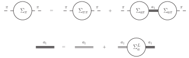
Figure 2: Schematic depiction of the contributions to the pion and $a_{1}$ self-energies, $\Sigma_{\pi}$, $\Sigma_{a_{1}}^{L}$. The bold $a_{1}$ line represents a resummed $a_{1}$ propagator in the longitudinal channel.

The 4D-longitudinal $AV$ polarization function can be constructed in a manner similar to the transverse mode but with intermediate $a_{1}$ and $\pi$ propagators (cf. Fig. 1),

$$\begin{split}\Pi_{A}^{L}(p^{2})&=\Sigma_{W}^{L}(p^{2})+\left(\Gamma_{A}^{L}(p^{2})\right)^{2}D_{A}^{L}(p^{2})\\ &+\frac{p^{2}F_{\pi}^{2}}{2}F^{2}(p^{2})D_{\pi}(p^{2})\,.\end{split}$$ (17)

The propagators read

$$D_{A}^{L}(p^{2}) = [M_{a_{1}}^{2}-\Sigma_{a_{1}}^{L}(p^{2})]^{-1},$$ (18)

$$D_{\pi}(p^{2}) = [p^{2}-M_{\pi}^{2}-\Sigma_{\pi}(p^{2})]^{-1}\,,$$ (19)

while the pion self-energy, $\Sigma_{\pi}$, contains a direct contribution and one with an intermediate $a_{1}$ propagator,

$$\Sigma_{\pi}(p^{2})\equiv\Sigma_{\pi\pi}(p^{2})+p^{2}\Sigma_{a\pi}^{2}(p^{2})D_{A}^{L}(p^{2})\ ,$$ (20)

see Fig. 2. The transition functions, $\Gamma_{A}^{L}$ and $F$, where the latter connects the $W$ boson to the pion, are given by:

$$\begin{split}\Gamma_{A}^{L}(p^{2})&=\frac{g_{\rho\pi\pi}F_{\pi}^{2}Z_{\pi}M_{a_{1}}}{2M_{\rho}}+\Sigma_{Wa_{1}}^{L}(p^{2}),\\ F(p^{2})&=1-\frac{\sqrt{2}}{F_{\pi}}\Sigma_{W\pi}(p^{2})\\ &+\frac{\sqrt{2}}{F_{\pi}}D_{A}^{L}(p^{2})\Gamma_{A}^{L}(p^{2})\Sigma_{a\pi}(p^{2}).\end{split}$$ (21)

A spectral function can also be defined for the 4D-longitudinal $AV$ polarization function: $\rho_{A}^{L}=-{\rm Im}\Pi_{A}^{L}/\pi$. As with the transverse mode, because of the the gauge symmetry, the EW self-energies can be expressed in terms of the meson self-energies,

$$\begin{split}\Sigma_{W}^{L}(p^{2})&=\frac{M_{\rho}^{2}Z_{\pi}^{2}}{g_{\rho\pi\pi}^{2}M_{a_{1}}^{2}}\Sigma_{a_{1}}^{L}(p^{2}),\\ \Sigma_{Wa_{1}}^{L}(p^{2})&=-\frac{M_{\rho}Z_{\pi}}{g_{\rho\pi\pi}M_{a_{1}}}\Sigma_{a_{1}}^{L}(p^{2}),\\ \Sigma_{W\pi}(p^{2})&=\frac{M_{\rho}Z_{\pi}}{g_{\rho\pi\pi}M_{a_{1}}}\Sigma_{a\pi}(p^{2})\ .\end{split}$$ (22)

This allows the spectral function to be written in a compact form in terms of the longitudinal $a_{1}$ propagator and the $\pi$ propagator,

$$\rho_{A}^{L}(p^{2})=-\frac{C_{A}}{\pi}{\rm Im}D_{A}^{L}(p^{2})-\frac{p^{2}F_{\pi}^{2}}{2\pi}{\rm Im}\left[D_{\pi}(p^{2})F^{2}(p^{2})\right]\ .$$ (23)

The coupling constant $C_{A}$ is the same as above, and $F$ is expressed in condensed form as

$$F(p^{2})=1-\frac{\sqrt{2}}{F_{\pi}}C_{A}^{1/2}\Sigma_{a\pi}(p^{2})D_{A}^{L}(p^{2})\,.$$ (24)

In all expressions above, $\Sigma_{a\pi}$ denotes the self-energy associated with the transition between the $a_{1}$ and $\pi$ states.

To calculate the $\rho$ and $a_{1}$ self-energies, we perform a loop expansion in addition to the derivative expansion associated with the Lagrangian, thereby including the diagrams depicted in Fig. 3. In the linear realization, the explicit $\sigma$ field precipitates the additional diagrams depicted in Fig. 4 for the $V$ and $AV$ channels. In both realizations, the $\pi a_{1}$ loop contribution to the $\rho$ self-energy is not included, as we have verified that it’s contribution to the vacuum spectral functions is negligible Hohler:2013ena . This then requires a modification of the $\rho\rho\pi\pi$ vertex coupling in the $\pi$-tadpole diagram in order to preserve gauge invariance. The self-energies, $\Sigma_{\pi\pi}$ and $\Sigma_{a\pi}$, are determined from the same diagrams as used in the $AV$ channel with the appropriate external legs.

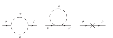
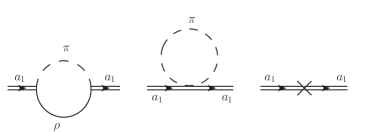
Figure 3: Feynman diagrams for the $\rho$ (upper row) and $a_{1}$ (lower row) self-energies; crosses denote counter-terms.

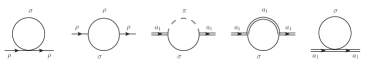
Figure 4: Additional diagrams contributing to the $V$ and $AV$ self-energies due to the inclusion of an explicit $\sigma$ field.

The loop integrals are rendered finite by dimensional regularization with the inclusion of suitable counter-terms. The latter are based on terms already present in the Lagrangian, thus preserving the chiral symmetry. Because of the momentum dependence of the divergences, higher derivative Lagrangian terms are also needed for the counter-terms. For the non-linear realization the counter-term Lagrangian needed to regulate the $V$ and $AV$ self-energies is given by:

$$\begin{split}\mathcal{L}_{\rm CT}&=\frac{\tilde{f}_{\pi}^{2}}{8}\left(\delta Z_{\pi}^{(2)}{\rm Tr}[D_{\mu}U^{\dagger}D^{\mu}U]\right.\\ &\left.+\frac{1}{4}\delta Z_{\pi}^{(4)}{\rm Tr}\left[\left(D_{\mu}D_{\nu}U^{\dagger}+D_{\nu}D_{\mu}U^{\dagger}\right)\right.\right.\\ &\left.\quad\quad\quad\times\left(D_{\mu}D_{\nu}U+D_{\nu}D_{\mu}U\right)\right]\\ &+\delta m_{\pi}^{2}{\rm Tr}[U+U^{\dagger}-2]\Big{)}-\frac{1}{2}\delta Z_{A}^{(2)}{\rm Tr}[F_{L}^{2}+F_{R}^{2}]\\ &+\delta Z_{A}^{(4)}{\rm Tr}\left[D^{\mu}F_{\mu\nu}^{L}D_{\lambda}F_{L}^{\lambda\nu}+D^{\mu}F_{\mu\nu}^{R}D_{\lambda}F_{R}^{\lambda\nu}\right]\\ &+\delta Z_{A}^{(6)}{\rm Tr}\left[D_{\mu}D^{\lambda}F_{\lambda\nu}^{L}D^{\mu}D_{\sigma}F_{L}^{\sigma\nu}\right.\\ &\quad\quad\quad\quad+D_{\mu}D^{\lambda}F_{\lambda\nu}^{L}D^{\nu}D_{\sigma}F_{L}^{\sigma\mu}\\ &\quad\quad\quad\quad+D_{\mu}D^{\lambda}F_{\lambda\nu}^{R}D^{\mu}D_{\sigma}F_{R}^{\sigma\nu}\\ &\left.\quad\quad\quad\quad+D_{\mu}D^{\lambda}F_{\lambda\nu}^{R}D^{\nu}D_{\sigma}F_{R}^{\sigma\mu}\right]\\ &+\delta\gamma^{(2)}\ {\rm Tr}[F_{L}UF_{R}U^{\dagger}]\\ &+\delta\gamma^{(4)}{\rm Tr}\left[D^{\mu}F_{\mu\nu}^{L}UD^{\lambda}F_{\lambda\nu}^{R}U^{\dagger}\right]\\ &+\delta\gamma^{(6)}{\rm Tr}\left[D^{\mu}D^{\lambda}F_{\lambda\nu}^{L}UD_{\mu}D_{\sigma}F_{R}^{\sigma\nu}U^{\dagger}\right.\\ &\left.\quad\quad\quad\quad+D^{\mu}D^{\lambda}F_{\lambda\nu}^{L}UD^{\nu}D^{\sigma}F_{\sigma\mu}^{R}U^{\dagger}\right]\ ,\end{split}$$ (25)

where

$$\begin{split}D_{\mu}F_{\lambda\nu}&=\partial_{\mu}F_{\lambda\nu}-ig\left[A_{\mu},F_{\lambda\nu}\right],\\ D_{\mu}D_{\lambda}F_{\nu\sigma}&=\partial_{\mu}\left(D_{\lambda}F_{\nu\sigma}\right)-ig\left[A_{\mu},D_{\lambda}F_{\nu\sigma}\right]\ .\end{split}$$ (26)

This can be expanded in terms of the physical fields as described for the MYM Lagrangian. The terms relevant for the self-energies are detailed in Appendix B. In the linear realization, we must add the counter-terms akin to the scalar potential

$$\mathcal{L}_{CT}=-\frac{\tilde{f}_{\pi}^{2}}{8}\left(\delta\mu^{2}{\rm Tr}\left[U^{\dagger}U\right]+\delta\lambda\frac{\tilde{f}_{\pi}^{2}}{4}{\rm Tr}\left[\left(U^{\dagger}U\right)^{2}\right]\right),$$ (27)

whose parameters are chosen so that the vacuum loop contribution from the lollipop diagrams in Fig. 11 is zero. This is equivalent to preventing the vacuum masses to be renormalized by these diagrams.

Each counter-term coupling has an infinite contribution needed to cancel off the divergences from the loops and a finite contribution, e.g. $\delta Z_{\pi}^{(2)}=\delta Z_{\pi}^{(2)\infty}+\bar{\delta Z}_{\pi}^{(2)}$ The finite contributions of the terms $\delta m_{\pi}$, $\delta Z_{\pi}^{(2)}$, and $\delta Z_{\pi}^{(4)}$ are determined by requiring that $M_{\pi}$ and $F_{\pi}$ are renormalized to their physical values. This is achieved by implementing the conditions $\Sigma_{\pi\pi}(M_{\pi}^{2})=0$, $\Sigma_{\pi\pi}^{\prime}(M_{\pi}^{2})=0$, and $\Sigma_{a_{1}\pi}(M_{\pi}^{2})=0$. The remaining six counter-term couplings are used to fit the vacuum spectral functions to experiment.

As discussed in Ref. Hohler:2013ena , we find that an agreement with the data can be achieved when the finite width of the $\rho$ is included in the calculation of the $a_{1}$ self-energy. This is done by using the fully resummed $\rho$ propagator in the $a_{1}$ self-energy’s $\pi\rho$ loop. However, this alone compromises the chiral properties at loop level which can be checked by employing a generalized form of PCAC Urban:2001ru ; Weinberg:1996kr ,

$$\int\frac{\rho_{A}^{L}}{s}ds=\frac{F_{\pi}^{2}}{2}\ .$$ (28)

We have verified that this equation is exactly satisfied for a zero-width $\rho$ in the chiral limit ($M_{\pi}=0$), facilitated by the following relations between the self-energies $\Sigma_{a_{1}}^{L}$, $\Sigma_{a\pi}$, and $\Sigma_{\pi\pi}$,

$$\Sigma_{a_{1}}^{L}=\frac{F_{\pi}^{2}}{2}\frac{M_{a_{1}}^{4}}{C_{A}}\frac{\Sigma_{\pi\pi}}{p^{2}}\,,\quad\quad\Sigma_{a\pi}=\frac{F_{\pi}}{\sqrt{2}}\frac{M_{a_{1}}^{2}}{C_{A}^{1/2}}\frac{\Sigma_{\pi\pi}}{p^{2}}\,.$$ (29)

For finite pion mass, deviations to these relations at order ${\cal O}(M_{\pi}^{2})$ develop due to pion tadpole contributions.

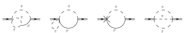
Figure 5: Vertex correction diagrams needed to recover PCAC in the presence of a pion-dressed $\rho$ propagator. The external legs represent $a_{1}$ or $\pi$ to generate the self-energies $\Sigma_{ij}$. The first three diagrams show the corrections to the left-hand vertex while the complete set includes the corrections to the right-hand vertex and to both simultaneously.

Using a broad $\rho$ in the loops of the $AV$ channel creates violations of Eq. (29) even in the chiral limit, upon integrating over the invariant-mass distribution of the $\rho$. It turns out that PCAC can be restored by including the vertex correction diagrams to the axial-vector self-energy shown in Fig. 5. These are constructed such that a sub-diagram which is part of the vertex correction has the same structure as the diagrams in the $\rho$ self-energy. Thus note that in the far right diagram, the 2 pions are in a relative $P$-wave to mimic a $\rho$ meson. In order to recover the necessary relations between the self-energies, the couplings between the external $a_{1}$/$\pi$ and the $3\pi$ (first and last diagram in Fig. 5) and $\rho 3\pi$ states (second diagram in Fig. 5), as well as the counter-terms (third diagram in Fig. 5), must be judiciously chosen, different from their Lagrangian values. This is expected since the full $\rho$ propagator is only a partial resummation. The deviation of the couplings from their Lagrangian values appropriately captures this resummation. More details on how this is implemented can be found in Appendix C.

With the use of the resummed $\rho$ propagator and accompanying vertex corrections, a new divergence is introduced into the $a_{1}$ self-energy which needs to be regulated. The problem arises from the fact that the sub-loops which are similar to the $\rho$ self-energy grow as $M^{6}$ for large invariant $\rho$ masses due to higher derivatives in the couplings. This growth, especially in the vertex corrections, is not compensated by the propagators resulting in divergent diagrams. To regulate these $a_{1}$ self-energy contributions in the spirit of effective field theory, we introduce a hard cut-off on the invariant $\rho$ mass when integrating over the $\rho$ spectral function by means of a dispersion relation, as detailed in Appendix C. The cut-off characterizes the scale where the theory breaks down, while the resulting vertex corrections still satisfy the relations of Eq. (29), thus preserving the chiral symmetry. We set the cut-off to $\Lambda_{\rm cut}=1.5$ GeV, based on the mass range where the $AV$ width starts to grow rapidly (larger values still allow fits of similar quality to the $\tau$-decay data, but become increasingly sensitive to the higher derivative terms).

Before turning to the fit of the vacuum $V$ and $AV$ spectral functions using the $\rho$ and $a_{1}$ propagators from MYM, two further ingredients beyond MYM are needed for a description of the data toward higher energies. The first is a contribution from the high-energy continuum, which saturates at a level corresponding to the perturbative quark-antiquark limit. Following our previous work Hohler:2012xd ; Hohler:2013ena , we adopt a chirally invariant continuum, i.e., identical for the two channels, with a functional form Shuryak:1993kg

$$\rho_{\rm cont}(s)=\frac{1}{8\pi^{2}}\left(1+\frac{\alpha_{s}}{\pi}\right)\frac{s}{1+\exp[(E_{0}-\sqrt{s})/\delta]}\ ,$$ (30)

which gradually ramps up to the expected high-energy perturbative limit. The second contribution is from the excited states, $\rho^{\prime}$ and $a_{1}^{\prime}$ which we include through a phenomenological Breit-Wigner resonance ansatz. These states chiefly represent 4- and 5-pion states coupling through resonant states, not captured by the MYM framework nor by the continuum. This is quite evident from the data in the $V$ channel, but more subtle in the $AV$ channel. Thus, the $\rho^{\prime}$ can be straightforwardly fitted to the data, while $a_{1}^{\prime}$ can be inferred from a quantitative analysis of Weinberg sum rules (WSRs), in the spirit of Ref. Hohler:2012xd . Clearly, the continuum and the resonant states cannot be uniquely separated.

Figure 6: Spectral functions in the vector (upper panel) and axial-vector (lower panel) channels as calculated from our MYM approach in non-linear realization (dashed lines), supplemented with a chirally invariant continuum (dotted lines) and first excited states (dash-dotted lines) Hohler:2012xd , compared to hadronic $\tau$-decay data Barate:1998uf .

Figure 7: Spectral functions in the vector (upper panel) and axial-vector (lower panel) channels as calculated from our MYM approach in linear realization (dashed lines), supplemented with a chirally invariant continuum (dotted lines) and first excited states (dash-dotted lines) Hohler:2012xd , compared to hadronic $\tau$-decay data Barate:1998uf .

Our final fit to the experimental spectral distributions as measured via hadronic $\tau$ decays by the ALEPH collaboration Barate:1998uf is displayed in Figs. 6 and 7 for the non-linear and linear realization, respectively. The values of the Lagrangian parameters used in the spectral function fits are listed in Table 1 while the values for the finite contribution to the counter-terms can be found in Table 2. We note that $M_{\rho}^{2}g_{\rho\pi\pi}^{(3)}$ is small compared to $g_{\rho\pi\pi}$ as required for a meaningful derivative expansion of the effective theory. The same can be said for the counter-terms when noting that the relevant energy scale of $\delta Z_{\pi}^{(4)}$ is $M_{\pi}$ rather than $M_{\rho}$ as with the other couplings. For the linear realization, the mass of the $\sigma$ field is needed, which was determined to be $M_{\sigma}=0.80$ GeV. In both realizations the cut-off scale is set to $\Lambda_{\rm cut}=1.5$ GeV and the continuum parameters ($\alpha_{s}$=0.5, $E_{0}$=1.55 GeV and $\delta$=0.22 GeV) have been slightly varied compared to Ref. Hohler:2012xd to optimize the fit.

	$g_{\rho\pi\pi}$	$g_{\rho\pi\pi}^{(3)}$	$M_{\rho}$	$M_{a_{1}}$	$M_{\sigma}$	$\Lambda_{\rm cut}$	$\alpha_{s}$	$E_{0}$	$\delta$
Non-Linear	6.01	0.02	0.86	1.20	–	1.5	0.5	1.55	0.22
Linear	6.36	-0.57	0.92	1.26	0.8	1.5	0.5	1.55	0.22

Table 1: Parameters used to obtain the vacuum fits to the experimental spectral functions in the vector and axial-vector channels in Figs. 6 and 7. The masses, cutoff and continuum parameters ($E_{0},\delta$) are in units of GeV, $g_{\rho\pi\pi}^{(3)}$ in GeV^-2.

	$\delta Z_{A}^{(2)}$	$\delta Z_{A}^{(4)}$	$\delta Z_{A}^{(6)}$	$\delta\gamma^{(2)}$	$\delta\gamma^{(4)}$	$\delta\gamma^{(6)}$	$\delta Z_{\pi}^{(2)}$	$\delta Z_{\pi}^{(4)}$	$\delta m_{\pi}$
Non-Linear	1.91	0.54	-0.06	1.76	-0.31	-0.08	1.94	14.70	0.06
Linear	1.14	0.72	-0.10	0.92	-1.13	0.19	1.14	10.06	0.05

Table 2: Counter-term parameters used to obtain the vacuum fits to the experimental spectral functions in the vector and axial-vector channels in Figs. 6 and 7. $\delta Z_{A}^{(4)}$, $\delta\gamma^{(4)}$, and $\delta Z_{\pi}^{(4)}$ are in units of GeV^-2; $\delta Z_{A}^{(6)}$ and $\delta\gamma^{(6)}$ are in units of GeV^-4, and $\delta m_{\pi}$ is in units of GeV.

Our fit within the loop-augmented MYM to the vacuum $AV$ spectral function presented here implies several specific features. One of them is illustrated in Fig. 8 where the “width” of the $a_{1}$, $\Gamma_{a}=-{\rm Im}\Sigma_{a}(s)/\sqrt{s}$, is plotted as a function of energy. In the vicinity of the resonance peak, $s\simeq 1-1.5$ GeV², it amounts to about 100-150 MeV, quite a bit smaller than the “apparent” width of the peak of $\sim$300-400 MeV. In order to generate sufficient spectral strength across the peak region, the real part of the $a_{1}$ self-energy needs to be tuned such that the real part of the inverse of the $a_{1}$ propagator, $s-M_{a_{1}}^{2}-{\rm Re}\Sigma_{a_{1}}$, stays in the vicinity of zero over an extended range in energy, cf. Fig. 9. This results in the spectral function being effectively given by $1/{\rm Im}\Sigma_{a_{1}}^{T}$, generating the necessary spectral strength through a sufficiently small ${\rm Im}\Sigma_{a_{1}}$ across the peak region. The remaining $\sim$10% peak strength is provided by the low-energy tails of the continuum and/or $a_{1}^{\prime}$ resonance, implying them to have non-vanishing 3-pion components (experimentally the peak region is known to be saturated by 3-pion states). As we already indicated in our previous work Hohler:2013ena , this construction is dictated by the lack of strength in the $AV$ coupling, $C_{A}$, which is fixed by the gauge principle, i.e., it cannot be adjusted independently from the $V$ coupling. Within the basic MYM setup, such a construction appears to be unavoidable; it is present in both non-linear and linear realiziations of chiral symmetry, although somewhat less pronounced in the latter . Earlier works which considered a global gauge symmetry do not have this feature as their couplings controlling the spectral height decouple in the $V$ and $AV$ channels. We will come back to this issue below, i.e., in how far it affects the robustness of the predictions for the finite-temperature spectral functions. As mentioned above, the strong growth of the width beyond $s=2$ GeV², which is also common to both realizations, indicates the break-down of the effective theory and is the basis for our choice of the sharp cut-off when integrating over pertinent spectral functions.

Figure 8: Imaginary part of the axial-vector self-energy for the non-linear (solid curve) and linear (dot-dashed curve) realization of MYM.

Figure 9: Real part of the inverse axial-vector propagator in vacuum for the non-linear (solid line) and linear (dot-dashed linear) realizations of chiral symmetry within MYM.

To further test the vacuum model, we calculate additional observables, including the radiative $a_{1}$ decay width, the $D/S$ ratio of the $a_{1}\to\rho\pi$ decay, the iso-vector $\pi\pi$ phase shift, and the pion electromagnetic (EM) formfactor. The radiative $a_{1}$ decay is found to be $\Gamma_{a_{1}\rightarrow\pi\gamma}$=244 keV for the non-linear realization and 42 keV for the linear case; especially the latter is quite a bit below the available datum extracted from proton-nucleus collisions, 640$\pm$246 keV Zielinski:1984au . These are tree-level results, as the hadronic loops in the current calculation, which potentially contribute to the radiative decay, vanish at the photon point. Additional hadronic loop corrections, which are not included in our scheme, might improve the situation, in particular pion exchange diagrams as discussed in Ref. Roca:2006am . For the $D/S$ ratio of the $a_{1}\rho\pi$ decays, loop corrections figure through the broad $\rho$ and associated vertex correction. When evaluated at $\sqrt{s}=1.23$ GeV, we find -0.101 for the non-linear realization and -0.052 for the linear realization. The Particle Data Group reports an average value of $0.062\pm 0.02$ (three out of the four listed measurements are around -0.12, while the fourth one is at $-0.043\pm 0.01$) Agashe:2014kda .

In extension of our previous work Hohler:2013ena , we here calculate the $\pi\pi$ phase shift and the pion EM formfactor, $|F_{\pi}|^{2}$, from our vector correlator and compare them to data Froggatt:1977hu ; Amendolia:1983di ; Amendolia:1984nz ; Barkov:1985ac , in Fig. 10. Both quantities agree reasonably well with experiment in both chiral realizations. In particular, the formfactor below the 2-pion threshold, extending into the space-like region, is not directly constrained by the vacuum spectral functions. The overall agreement with these data suggests that the vacuum model has reasonably well incorporated the relevant physics.

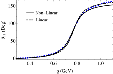
Figure 10: Upper panel: $\pi\pi$ scattering phase shift in the iso-vector channel compared with experimental measurements (points) Froggatt:1977hu . Lower panel: Pion EM formfactor compared to experimental measurements (points) Amendolia:1983di ; Amendolia:1984nz ; Barkov:1985ac . In each panel, results of the non-linear (solid curve) and linear (dashed curve) realization are shown.

IV In-medium spectral functions

At finite temperature, the breaking of Lorentz symmetry splits the 4D-transverse polarization functions at finite 3-momentum into 3D-transverse, $\Pi^{\perp}$, and longitudinal, $\Pi^{\parallel}$, components. The polarization functions in $V$ and $AV$ channels can thus be decomposed as

$$\Pi^{\mu\nu}_{V,A}\left(p_{0},|\vec{p}|\right)=\Pi^{\perp}_{V,A}P_{T}^{\mu\nu}+\Pi^{\parallel}_{V,A}P_{L}^{\mu\nu}+\Pi^{L}_{V,A}\frac{p^{\mu}p^{\nu}}{p^{2}}\ ,$$ (31)

with the standard 3D-transverse ($P_{T}^{\mu\nu}$) and -longitudinal ($P_{L}^{\mu\nu}$) projection operators

$$P_{T}^{\mu\nu} = \delta^{ij}-\frac{p^{i}p^{j}}{|\vec{p}|}\,,$$ (32)

$$P_{L}^{\mu\nu} = -g^{\mu\nu}+\frac{p^{\mu}p^{\nu}}{p^{2}}-P_{T}^{\mu\nu}\,.$$ (33)

The spectral functions follow from the usual definitions, $\rho_{V,A}^{\perp,\parallel}=-{\rm Im}\Pi_{V,A}^{\perp,\parallel}/\pi$. As in vacuum, the gauge symmetry renders the spectral functions of a form suggestive of (A)VMD, thus Eq. (15) holds for both 3D polarizations.

IV.1 Finite-$T$ Vector Spectral Function

To calculate the in-medium spectral function, the $\rho$ self-energies at finite temperature need to be determined. The same loop diagrams that were considered in vacuum (cf. upper panel in Fig. 3) are evaluated using standard thermal field theory techniques. In addition, the $\pi a_{1}$ loop needs to be accounted for to maintain the chiral properties at finite $T$, cf. Fig. 11. The explicit forms of the loop integrals of each contribution (after the Matsubara sums are evaluated) are collected in Appendix D. The pion tadpole diagram contributes only to the real part while the other loop diagrams include the effects from both the unitarity and Landau cuts, representing the $\rho$ decaying into thermal hadrons and $\rho$ scattering off a thermal $\pi$ or $a_{1}$, respectively, as depicted in Fig. 12. The linear realization additionally requires the inclusion of the lollipop diagrams of Fig. 11 where the shaded loop indicates the sum of a contact interaction and in-medium $\pi$ and $\sigma$ loops. These sets of diagrams do not contribute in vacuum as they are set to zero to properly regularize the pion mass to its physical value. The thermal and vacuum widths of the pion and $a_{1}$ states within the loops are not taken into account.

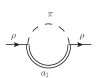
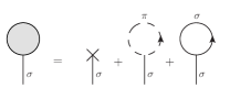
Figure 11: Diagrams added for in-medium self-energy calculations. (a) $\pi a_{1}$ loop which contributes to the finite-temperature $\rho$ self-energy. (b) $\sigma$ lollipop diagrams which contribute to the finite-temperature hadronic self-energies. (c) Detail of the contributions of the shaded loop in (b). The cross in the first diagram refers to the tree level contributions.

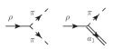
(a) Unitarity cut (decay)

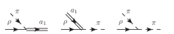
(b) Landau cut (scattering)

Figure 12: Diagrams of the processes contributing to broadening the $\rho$ spectral function in medium. The last two diagrams for the Landau contribution are only present when the $\rho$ is space-like.

The resulting vector spectral functions for the non-linear realization are presented in Fig. 13 at different temperatures with total momentum $|\vec{p}|=0$ ($\rho^{\perp}$ and $\rho^{\parallel}$ are degenerate under this condition). We have analytically verified that there is no shift in $M_{\rho}^{2}$ at order $T^{2}$ for low $T$. This is confirmed in the full numerical calculation by the lack of an appreciable shift in the spectral peak location. Therefore, as temperature increases, the $\rho$ spectral function essentially broadens, although not by much. The broadening is caused by the Bose-enhanced $\rho$ decay into $\pi\pi$ (unitarity cut of $\pi\pi$ loop) and by its scattering off a thermal $\pi$ into an $a_{1}$ (Landau cut of the $\pi a_{1}$ loop). The width increase of up to $\sim$45 MeV at $T=160$ MeV at the spectral peak is somewhat smaller than in similar calculations in Refs. Rapp:1999qu ; Urban:2001uv , due to a zero-width $a_{1}$ resonance and a larger $a_{1}$ mass, respectively. The small peak at $M=M_{a_{1}}-m_{\pi}=1.06$ GeV is a threshold effect due the sharp $a_{1}$ and pion masses: beyond this mass thermal pions cannot excite an $a_{1}$ anymore. The inclusion of the hadrons’ widths in future calculations will smoothen this feature out.

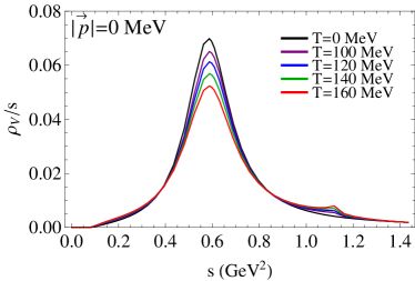
Figure 13: Vector spectral function in the non-linear realization at zero momentum for several temperatures.

Spectral functions at different momenta and a fixed temperature of $T=150$ MeV are shown in Fig. 14. The degeneracy between the 3D-transverse and longitudinal components for $|\vec{p}|=0$ is now lifted; the resonance peak in the 3D-transverse channel shifts to slightly higher energies while it moves downward in the 3D-longitudinal one. The amount of breaking between the channels increases with momentum. The divergence in $\rho^{\perp}/s$ at small invariant masses arises since $\Sigma_{\rho}^{\perp}$ is finite at the photon point. On the other hand, the longitudinal spectral functions vanish at the photon point. The results for the linear realization are very similar and thus are not presented here.

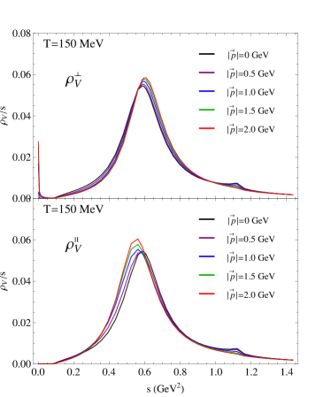
Figure 14: Vector spectral function in non-linear realization at $T$=150 MeV for various 3-momenta. Upper panel: 3D-transverse channel. Lower panel: 3D-longitudinal channel.

IV.2 Finite-$T$ Axial-Vector Spectral Function

In the present work, we focus on the case of $|\vec{p}|=0$, therefore $\rho_{A}^{\perp}$ and $\rho_{A}^{\parallel}$ are degenerate and equal to $\rho_{A}^{T}$. The in-medium $a_{1}$ self-energy is calculated using the same diagrams as in the vacuum, but keeping the vacuum dressing of the $\rho$ propagator. The vertex corrections are also evaluated in their vacuum form to be consistent with the level of approximation that intermediate particles develop no thermal widths in the current calculations. The explicit forms of the loop integrals for each contribution are collected in Appendix D. Both the unitarity and Landau cut processes, associated with each loop, ${\it e.g.}$, $a_{1}\rightarrow\rho\pi$ decay and $a_{1}\pi\rightarrow\rho$ scattering, respectively, are accounted for. As in the vector channel, the medium contribution from the lollipop diagram of Fig. 11 with appropriate external legs is additionally needed for the finite-temperature $a_{1}$ self-energy in the linear realization.

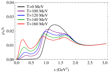
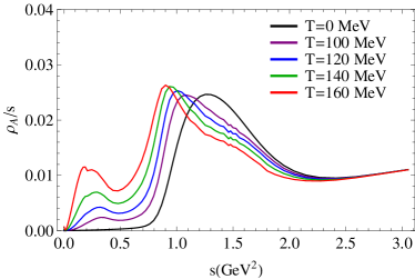
Figure 15: Finite-$T$ axial-vector spectral functions at $|\vec{p}|=0$ in non-linear (upper panel) and linear realizations (lower panel).

The resulting $AV$ spectral functions are presented at several temperatures in Fig. 15 for both realizations of chiral symmetry. Several common features emerge which may be considered as robust. First, the $a_{1}$ resonance peak noticeably shifts to lower masses with increasing temperature. This is caused by both the attractive tadpole contributions and the in-medium broadening of the $\pi\rho$ unitarity cut. This is different from the $\rho$ case where the in-medium tadpoles generate repulsion. Both realizations also develop a secondary peak or shoulder at somewhat higher masses, around $s\simeq 1.6$-1.7 GeV². In the non-linear version the double-peak structure is rather broad while in the linear version more strength is in the lower and somewhat narrower peak. These differences can be traced back to the behavior of the real part of the inverse $AV$ propagator in vacuum (recall Fig. 9), where the non-linear version exhibits an extended region close to zero while the linear one has a zero crossing leading to a well-defined peak. The second robust feature is the development of a marked low-mass peak around $\sqrt{s}\simeq 0.5$ GeV, caused by the scattering of an off-shell $a_{1}$ off thermal pions into the $\rho$ resonance. This process is related to the well-known “chiral mixing” Dey:1990ba , but evaluated with full thermal and finite-pion mass kinematics (see also Ref. Steele:1996su ), which results in a peak at masses significantly lower than the nominal $\rho$ mass.

Figure 16: Axial-vector spectral function at $T$=120 MeV with $\Lambda_{\rm cut}$=1.5 GeV (solid curve) and $\Lambda_{\rm cut}$=1.7 GeV (dashed curve).

To further scrutinize possible model dependencies, let us return to the question of the cut-off of the integration over the $\rho$ spectral strength when computing the real part of the $a_{1}$ self-energy from a dispersion integral. In the context of the vacuum calculations, we argued $\Lambda_{\rm cut}=1.5$ GeV to be a reasonable choice, to suppress (unphysical) high-energy contributions to the imaginary part of the $a_{1}$ self-energy which rapidly increase due to higher-derivative contributions from large invariant $\rho$ masses. To study the effect of variations in $\Lambda_{\rm cut}$ on the finite-$T$ results, we compare in Fig. 16 the $a_{1}$ spectral function in the non-linear realization at $T=120$ MeV with two different cut-offs, 1.5 GeV and 1.7 GeV. (The counter-term parameters are readjusted for the larger cut-off to recover a vacuum fit.) For masses below 1 GeV, the impact is minimal, but becomes significant above. Specifically, the larger cut-off produces additional repulsion in $AV$ self-energy in the region of the vacuum $a_{1}$ peak and beyond, leading to a noticeable suppression in spectral strength especially around $s\simeq 1.7$ GeV, erasing the higher-mass bump. Even though the $\Lambda_{\rm cut}=1.7$ GeV bears some resemblance with the finite-$T$ results of the linear realization, the variation must be considered as a model dependence caused by the “fragility” of the real part in the non-linear realization, another symptom for the breakdown of the theory as higher-order derivative contributions become appreciable. The high-energy behavior is better controlled with the lower cut-off which we therefore deem preferable.

V Quantifying the Approach to Chiral Symmetry Restoration

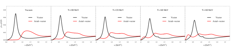
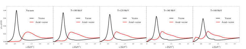
Figure 17: Temperature progression of vector and axial-vector spectral functions. Upper panel: Non-linear realization. Lower panel: Linear realization.

Let us start by visually inspecting the temperature progression of the vector vs. axialvector spectral functions, cf. Fig. 17 (for better clarity of the medium effects we did not include the contributions from the excited states). The stability of the $\rho$ mass together with the downward shift of the $a_{1}$ indicate an approach to chiral restoration that is characterized by “burning off” the chiral mass splitting, rather than a common mass drop. This mechanism is quite consistent with our independent recent analysis of Weinberg and chiral sum rules, where an in-medium hadronic many-body $\rho$ spectral function (that describes dilepton data) and chiral order parameters from lattice QCD were used as input Hohler:2013eba . Similar patterns for the $\rho\pi a_{1}$ system have also been found in Refs. Song:1993af ; Urban:2001uv .

While the suggestive trends discussed above are promising, a key objective of a microscopic approach, as the one pursued here, is to quantify the amount of restoration. The natural measure of this are chiral order parameters, such as the chiral condensate, $\langle\bar{q}q\rangle$, and the pion decay constant, $F_{\pi}^{2}$. In this section, we elaborate how the $T$ dependence of these two quantities can be calculated within MYM and discuss the results.

V.1 Pion Decay Constant

The most direct calculation of $F_{\pi}^{2}(T)$ is following the same procedure as in vacuum, i.e., from its definition as the effective coupling between the pion and the axial-vector current. Alternatively, and more indirectly, we employ the first Weinberg sum rule by inserting the finite-$T$ vector and axial-vector spectral as calculated above. We will carry out both methods for both realizations.

In vacuum, the $AV$ longitudinal channel serves as a measure of the chiral properties of the model through PCAC and has been used as guideline for identifying vertex corrections necessary to preserve the symmetry. At finite temperature, this channel can be used to extract the temperature dependence of $F_{\pi}^{2}$ by using Eq. (28). The key ingredients are the temperature effects on the self-energies $\Sigma_{a_{1}}^{L}$, $\Sigma_{\pi a}$, and $\Sigma_{\pi\pi}$. These are calculated in the same manner as discussed above for the $a_{1}$ transverse self-energy with $\rho_{A}^{L}$ given by Eq. (23), and the loop integrals for each contribution written out in Appendix D.

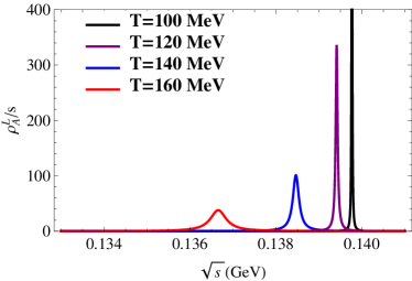
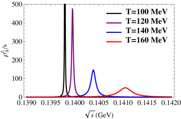
Figure 18: Pion spectral function at finite temperature in the non-linear (upper panel) and linear realization (lower panel).

The dominant contribution to the longitudinal spectral function is the pion spectral peak, displayed in Fig. 18 for several temperatures. In vacuum, it is a delta function (not shown) located at the physical pion mass of $139.6$ MeV, while the $T=100$ MeV peak extents beyond the plot. The narrowness of the peak implies the imaginary parts of the self-energies included in $\rho_{A}^{L}$ to be small such that $F_{\pi}^{2}(T)$ can be well approximated by

$$F_{\pi}^{2}(T)=F_{\pi}^{2}(0)\left.{\rm Re}\left[F^{2}\right]\left(1-\partial{\rm Re}\Sigma_{\pi}/\partial p^{2}\right)^{-1}\right|_{p^{2}=M_{\pi}^{2}(T)}\,,$$ (34)

where $F$ is given by Eq. (24). The resulting temperature dependence of $F_{\pi}^{2}$ is shown by the solid lines in the upper and lower panels of Fig. 19 for non-linear and linear realizations, respectively. It turns out to be quite comparable between the two realizations, being consistent with chiral low-temperature expansions and reduced by up to 15-17% at $T=160$ MeV.

The mechanism which leads to this reduction can be more readily understood in the non-linear realization. The reduction is controlled by ${\rm Re}\Sigma_{a\pi}$ due to increasing positive values. As we saw with the mass shifts in the $\rho$ and $a_{1}$ spectral peaks, there are two contributions which can affect this, one from the loops and one from the tadpoles. The case with $\Sigma_{a\pi}$ is more similar to $\Sigma_{\rho}$ where the loops and tadpoles provide opposing contributions, with attractive loops and repulsive tadpoles. As temperature increases, the two competing sides almost balance each but with the repulsive terms winning out.

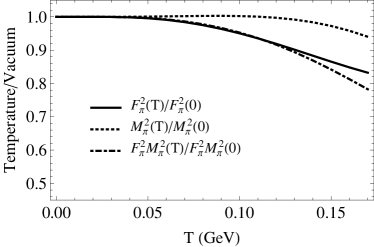
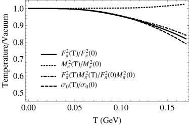
Figure 19: Upper panel: Temperature dependence of $F_{\pi}^{2}$, $M_{\pi}^{2}$, and their product for the non-linear realization. Lower panel: Temperature dependence of $F_{\pi}^{2}$, $M_{\pi}^{2}$ and $\sigma_{0}$ for the linear realization.

Complementary to the field theory approach is the calculation of $F_{\pi}$ from the first Weinberg sum rule (WSR) Weinberg:1967kj , which relates the first negative moment of the $V$ minus $AV$ spectral function to $F_{\pi}^{2}$. For vanishing 3-momentum ($|\vec{p}|=0$) one has

$$\int\left(\rho_{V}^{T}-\rho_{A}^{T}\right)s^{-1}ds=\frac{F_{\pi}^{2}}{2}\ .$$ (35)

Ideally, one would evaluate this equation with just the in-medium $V$ and $AV$ spectral functions as calculated above. However, already in vacuum the WSRs are not satisfied when only the $\rho$ and $a_{1}$ contributions are accounted for. Excited states, $\rho^{\prime}$ and $a_{1}^{\prime}$, and/or different continuum contributions, are essential to quantitatively satisfy the WSRs, see, e.g., the recent discussion in Ref. Hohler:2012xd . Since the calculation of medium modifications of the excited states is currently beyond the scope of MYM, we will approximate their contribution by a $T$ independent constant added to the left-hand side of the Eq. (35). This constant is chosen so that the vacuum sum rule is satisfied. Assuming the constant to be temperature independent will presumably overestimate $F_{\pi}^{2}$ in the medium as an expected chiral restoration of the excited states would lead to a further reduction (this effect will become stronger for the higher WSRs which involve higher moments in $s$). Put differently, we only evaluate the effects of chiral restoration due to in-medium effects on the $\rho$ and $a_{1}$ states. The temperature dependence of $F_{\pi}^{2}$ calculated in this manner is depicted in Fig. 20. While it is rather consistent between the two realizations, its reduction with temperature is more pronounced compared to the evaluation from the longitudinal $AV$ spectral function. The stronger reduction can have two principal sources: a lack of vector spectral strength and/or too much axial-vector spectral strength; low-mass strength, in particular, affects the negative moment of the first WSR. An obvious origin of missing strength in the vector channel is the in-medium dressing of the pions, which is known to generate a low-mass enhancement in the $\rho$ spectral function especially through the unitarity cut, but also through the Landau cut at very low mass (although suppressed by small pion widths at small 3-momenta). In addition, in the current calculation, the $\pi a_{1}$ Landau cut only includes a sharp (i.e., zero-width) $a_{1}$. A more complete calculation of these contributions, which requires further vertex corrections to preserve gauge symmetry, would induce extra broadening in the $\rho$ spectral peak. At the same time, pion broadening is expected to affect less the low-mass strength of the $a_{1}$ spectral function. On the other hand, increased imaginary parts at finite $T$ in the $a_{1}$ self-energy could, in fact, lead to a suppression of the $AV$ spectral function in the energy regime around $s>1$ GeV² (as illustrated in Fig. 16 in the context of (spurious) vacuum contributions). Thus, it is conceivable that future calculations, involving additional finite-width effects on all particles in the loops, will increase (decrease) the $V$ ($AV$) contribution to the WSRs and “stabilize” them.

Figure 20: Temperature dependence of $F_{\pi}^{2}$ relative to its vacuum value calculated from the first WSR using the non-linear (solid curve) and linear realization (dashed curve).

V.2 Chiral Condensate

In the linear realization, $\langle\bar{q}q\rangle(T)$ can be directly related to the $T$ dependence of the scalar-field condensate, $\sigma_{0}(T)$. This is determined without relying on any of the specific spectral functions of the field theory, by minimizing the scalar potential with respect to $\sigma_{0}$. Diagrammatically, this is equivalent to setting the lollipop diagrams of Fig. 11 to zero and solving for $\sigma_{0}$ at each temperature. However, this procedure is not consistent with the 1-loop treatment that we implement throughout the present work. The appropriate temperature correction to the vacuum $\sigma_{0}$ at the 1-loop level is rather obtained from the lollipop diagrams alone, i.e., not solving for $\sigma_{0}$. One has

$$\frac{\sigma_{0}(T)}{\sigma_{0}(0)}=1+\frac{1}{\sigma_{0}M_{\sigma}^{2}}\left(\Sigma_{\rm lolli}^{\pi}+\Sigma_{\rm lolli}^{\sigma}\right)\ ,$$ (36)

with the $\Sigma_{\rm lolli}$’s quoted in Appendix D. The contributions of these diagrams are related to the scalar densities of the pion and sigma, respectively. Therefore, this procedure is similar to the standard density expansion where the reduction of the condensate is driven by the increase of the density of the medium particles (“vacuum cleaner”). The resulting temperature dependence of $\sigma_{0}$ is shown as the dashed line in Fig. 19. It exhibits a smooth decrease of up to $\sim$18% at $T=160$ MeV.

In the non-linear realization, the chiral condensate cannot be directly calculated. However, we can take recourse to calculations of $F_{\pi}(T)$ and $M_{\pi}(T)$ to find the $T$ dependence of the chiral condensate through the Gellmann-Oakes-Renner (GOR) relation,

$$\langle\bar{q}q\rangle(T)/\langle\bar{q}q\rangle(0)=M_{\pi}^{2}(T)F_{\pi}^{2}(T)/M_{\pi}^{2}(0)F_{\pi}^{2}(0)\,.$$ (37)

The temperature dependence of $M_{\pi}$ is determined from the zero of the real part of the inverse pion propagator in Eq. (19). We find a very slightly increasing trend at low temperatures in both realizations (in line with low-$T$ chiral expansions Gasser:1986vb ), which, however, turns around into a $\sim$5% attraction in the nonlinear case at $T=160$ MeV, while the linear case reaches a 2% repulsion at this temperature (see dotted lines in Fig. 19). When evaluating the quark condensate with GOR, the two realizations slightly differ because of the added repulsion in pion self-energy for the linear realization. Furthermore, in the linear realization, the scalar condensate calculated via either GOR or directly gives slightly different results particularly at higher temperatures. This stems from the differences between performing a loop expansion rather than a formal $T^{2}$ expansion.

Nevertheless, our overall findings for the temperature dependence of the chiral order parameters give a fairly consistent picture between the two realizations, indicating that their reduction in temperature is a robust feature accompanying the approach toward degeneracy in the spectral functions. Quantitatively, when directly evaluated from the low-energy properties of the longitudinal $AV$ spectral function, the reduction reaches up to $\sim$15-20% at $T=160$ MeV. It is about twice as large when evaluated with the first WSR, which we tentatively attribute to neglecting higher-order width effects expected to impact the $V$ channel more strongly than the $AV$ one, thus taming the reduction.

VI Hadronic Mechanisms of Chiral Symmetry Restoration

In this section we put our work into a broader context and identify future studies to improve our understanding of hadronic mechanisms leading to chiral restoration.

Hadronic degeneracy is well established in mean-field approaches of chiral effective hadronic theories, where the masses of, e.g., the $\pi$-$\sigma$ and $\rho$-$a_{1}$, degenerate in the chirally restored phase Pisarski:1995xu ; Bochkarev:1995gi ; Bilic:1997sh ; Petropoulos:1998gt ; Struber:2007bm . It remains, however, rather challenging to conduct these calculations beyond the mean-field level under the inclusion of finite-width effects which are essential to obtain realistic spectral functions. As we discussed above, this is a non-trivial task for the axial-vector spectral function already in vacuum, at least for local-gauge approaches. On the other hand, our finite-temperature calculations presented above are carried out in a loop expansion which does not implement in-medium changes of the underlying hadronic coupling constants. The next step should thus aim at a self-consistent treatment.

Let us focus on the linear realization of MYM, which is more readily amenable for treating the transition region. At the mean-field level, the masses and couplings are explicit functions of the condensate $\sigma_{0}$. We may thus identify for each mass and coupling a contribution which is finite for $\sigma_{0}=0$ and one which vanishes and interpret the latter as due to spontaneous symmetry breaking. As $\sigma_{0}$ is driven to lower values, the symmetry breaking contributions “burn” off. The seed for this mechanism is already inherent in our calculations, as confirmed by the results presented above in terms of the $a_{1}$ mass approaching the $\rho$ mass and the accompanying reduction in the scalar condensate. Extending this all the way to the restored phase, the bare masses of the chiral partners, $(M_{\rho},M_{a_{1}})$ and $(M_{\pi},M_{\sigma})$, will become identical as can be gleaned from Eq. (II). For the self-energies, at the one loop level, this implies that the $\rho\to\pi\pi$ and pion tadpole of Fig. 3 degenerate with the $a_{1}\to\sigma\pi$ loop (third diagram in Fig. 4) and the pion tadpole for the $a_{1}$ (second diagram in Fig. 3), while all other diagrams vanish, in particular, the $\pi\rho$ loop in the $a_{1}$ self-energy and the $\pi a_{1}$ loop in the $\rho$ self-energy (since the $\rho\pi a_{1}$ coupling vanishes for $\sigma_{0}=0$). A similar analysis holds for the $\pi$ and $\sigma$ self-energies. With $\pi$-$\sigma$ degeneracy, this implies the $V$ and $AV$ spectral functions to degenerate as well. This analysis suggests that the mechanism of chiral mixing, which is the leading effect in the low-$T$ limit induced by the $\pi\rho a_{1}$ coupling, vanishes at the restoration point, while a central role is taken by the $\pi$-$\sigma$ degeneracy and the “burning” of the chiral mass splitting. In this context, it is interesting to note that a recent lattice computation of the correlation functions of the nucleon and its chiral partner, the $N^{*}(1535)$, also suggests that the main effect of chiral restoration at finite temperature is a vanishing of the mass splitting while the nucleon mass itself is little affected Aarts:2015mma .

In practice, a self-consistent field-theoretic implementation with realistic (broad) spectral distributions remains challenging. The evaluation of $\sigma_{0}(T)$ from solving the gap equation needs to be accompanied by higher thermal-loop calculations. This will require the dressing of all internal particles with their thermal widths. The dressed propagators will necessarily precipitate compensating vertex corrections to maintain the symmetries, some of which will be similar to the types considered here. To be able to use the full temperature dependence of $\sigma_{0}$ in the vertices may also require a resummation of the vertices, or at least casting the vertex corrections in terms of the relevant self-energies.

To make contact with experimental measurements of dilepton emission through the vector channel, the effects of baryons need to be accounted for. Their quantitative importance in the experimental context is likely to alter the predicted pseudo-critical temperature, but they might not introduce a qualitatively new mechanism of chiral restoration, relative to what our pion gas findings in the present analysis suggest. In fact, our aforementioned analysis of QCD and WSRs, using realistic in-medium spectral functions, indicated that chiral-mass burning is compatible with dilepton experiments Hohler:2013eba .

VII Conclusion

Based on a Massive Yang-Mills implementation of vector and axial-vector mesons into the chiral pion Lagrangians which yields vacuum spectral functions compatible with experiment, we have calculated their modifications in a hot pion gas. A key feature of such approaches is that they enable the evaluation of chiral order parameters within the same framework, and thus provide connections between chiral restoration and spectral modifications (which can be measured in dilepton experiments). Toward this end, we have carried out a temperature loop expansion encompassing tadpole and 2-particle loop diagrams as well as vertex corrections associated with the vector and chiral Ward identities. As a check of the robustness of our predictions, we have evaluated both spectral functions and chiral order parameters in both the linear and non-linear realization of chiral symmetry in the pion Lagrangian. A fair consistency of the two methods for both order parameters and spectral functions is found. While the $\rho$ meson spectral function undergoes a modest finite-temperature broadening with a stable pole mass (in agreement with previous calculations of a similar kind), the in-medium $a_{1}$ spectral function exhibits a significant mass shift toward the $\rho$ meson. These medium effects are accompanied by a 15-20% reduction in the scalar condensate and pion decay constant at $T$=160 MeV, suggesting that the reduction in the $a_{1}$ mass signals a mechanism of chiral symmetry restoration whereby chiral mass splittings are burned off. A similar mechanism also emerged from QCD and Weinberg sum rule analyses with full hadronic many-body $\rho$ spectral functions, and from recent thermal lattice-QCD computations of the correlation functions of the nucleon and its chiral partner, $N^{*}(1535)$. We have conjectured that such a mechanism is quite different from the so-called chiral mixing and rather involves the degeneracy in the scalar-pseudoscalar channel as a critical ingredient. The full embodiment of this mechanism, ultimately leading to spectral degeneracy in the restored phase, requires the self-consistent implementation of additional medium effects beyond the loop expansion, associated with dressed in-medium propagators (including baryonic effects), accompanying vertex corrections, and a simultaneous solution of the chiral gap equation (which is more naturally done in the linear realization of MYM). Work in these directions is in progress.

Appendix A Lagrangian couplings for relevant MYM vertices

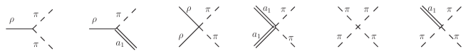
Figure 21: Tree level vertices for both the non-linear and linear realizations used in calculations in this paper.

In this appendix, we detail the vertex couplings which were utilized in the calculations of this paper. They follow from the MYM Lagrangian, Eq. (1), upon expansion in the physical fields, as described in Sec. II.

We begin with the relevant vertices of the non-linear realization, diagrammatically depicted in Fig. 21. The resulting Lagrangian terms are as follows:

$$\mathcal{L}_{\rho\pi\pi}^{\rm nLin} = g_{\rho\pi\pi}\,\rho_{\mu}\cdot\pi\times\partial^{\mu}\pi+g_{\rho\pi\pi}^{(3)}\,\rho_{\mu\nu}\cdot\partial^{\mu}\pi\times\partial^{\nu}\pi$$ (38)

$$\mathcal{L}_{\rho\pi a_{1}}^{\rm nLin} = C\,\rho_{\mu}\cdot\pi\times a^{\mu}+D\,\rho_{\mu\nu}\cdot\pi\times a^{\mu\nu}+E\,\rho_{\mu}\cdot\partial_{\nu}\pi\times a^{\mu\nu}+F\,\rho_{\mu\nu}\cdot\partial^{\mu}\pi\times a^{\nu}$$ (39)

$$\mathcal{L}_{\rho\rho\pi\pi}^{\rm nLin} = \alpha_{1}\left(\pi\cdot\rho_{\mu}\,\pi\cdot\rho^{\mu}-\pi\cdot\pi\,\rho_{\mu}\cdot\rho^{\mu}\right)+\alpha_{2}\left(\pi\cdot\rho_{\mu\nu}\,\pi\cdot\rho^{\mu\nu}-\pi\cdot\pi\,\rho_{\mu\nu}\cdot\rho^{\mu\nu}\right)$$

$$+\alpha_{3}\left(\partial_{\mu}\pi\cdot\rho^{\mu\nu}\,\pi\cdot\rho_{\nu}-\partial_{\nu}\pi\cdot\rho^{\mu\nu}\,\pi\cdot\rho_{\mu}\right)+\alpha_{4}\left(\partial_{\mu}\pi\cdot\rho_{\nu}\,\pi\cdot\rho^{\mu\nu}-\partial_{\nu}\pi\cdot\rho_{\mu}\,\pi\cdot\rho^{\mu\nu}\right)$$

$$+\alpha_{5}\,\partial_{\mu}\pi\cdot\rho_{\nu}\,\partial^{\nu}\pi\cdot\rho^{\mu}+\alpha_{6}\,\partial_{\mu}\pi\cdot\rho^{\mu}\,\partial_{\nu}\pi\cdot\rho^{\nu}+\alpha_{7}\left(\rho_{\mu}\cdot\rho^{\mu\nu}\,\pi\cdot\partial_{\nu}\pi-\rho_{\nu}\cdot\rho^{\mu\nu}\,\pi\cdot\partial_{\mu}\pi\right)$$

$$+\alpha_{8}\left(\partial_{\mu}\pi\cdot\partial^{\mu}\pi\,\rho_{\nu}\cdot\rho^{\nu}-\partial_{\mu}\pi\cdot\partial_{\nu}\pi\,\rho^{\mu}\cdot\rho^{\nu}-\partial_{\mu}\pi\cdot\rho_{\nu}\,\partial^{\mu}\pi\cdot\rho^{\nu}\right)$$

$$\mathcal{L}_{a_{1}a_{1}\pi\pi}^{\rm nLin} = \beta_{1}\left(\pi\cdot a_{\mu}\,\pi\cdot a^{\mu}-\pi\cdot\pi\,a_{\mu}\cdot a^{\mu}\right)+\beta_{2}\left(\pi\cdot a_{\mu\nu}\,\pi\cdot a^{\mu\nu}-\pi\cdot\pi\,a_{\mu\nu}\cdot a^{\mu\nu}\right)$$

$$+\beta_{3}\left(\partial_{\mu}\pi\cdot a^{\mu\nu}\,\pi\cdot a_{\nu}-\partial_{\nu}\pi\cdot a^{\mu\nu}\,\pi\cdot a_{\mu}\right)+\beta_{4}\,\partial_{\mu}\pi\cdot a_{\nu}\,\partial^{\nu}\pi\cdot a^{\mu}$$

$$+\beta_{5}\,\partial_{\mu}\pi\cdot a^{\mu}\,\partial_{\nu}\pi\cdot a^{\nu}+\beta_{6}\left(a_{\mu}\cdot a^{\mu\nu}\,\pi\cdot\partial_{\nu}\pi-a_{\nu}\cdot a^{\mu\nu}\,\pi\cdot\partial_{\mu}\pi\right)$$

$$+\beta_{7}\left(\partial_{\mu}\pi\cdot\partial^{\mu}\pi\,a_{\nu}\cdot a^{\nu}-\partial_{\mu}\pi\cdot\partial_{\nu}\pi\,a^{\mu}\cdot a^{\nu}-\partial_{\mu}\pi\cdot a_{\nu}\,\partial^{\mu}\pi\cdot a^{\nu}\right)$$

$$\mathcal{L}_{\pi\pi\pi\pi}^{\rm nLin} = \gamma_{1}\left(\pi\cdot\partial_{\mu}\pi\,\pi\cdot\partial^{\mu}\pi-\pi\cdot\pi\,\partial_{\mu}\pi\cdot\partial^{\mu}\pi\right)+\gamma_{2}\left(\partial_{\mu}\pi\cdot\partial_{\nu}\pi\,\partial^{\mu}\pi\cdot\partial^{\nu}\pi-\partial_{\mu}\pi\cdot\partial^{\mu}\pi\,\partial_{\nu}\pi\cdot\partial^{\nu}\pi\right)$$ (43)

$$+\gamma_{3}\,\pi\cdot\pi\,\pi\cdot\pi$$

$$\mathcal{L}_{a_{1}\pi\pi\pi}^{\rm nLin} = \delta_{1}\left(a_{\mu}\cdot\pi\,\partial^{\mu}\pi\cdot\pi-a_{\mu}\cdot\partial^{\mu}\pi\,\pi\cdot\pi\right)+\delta_{2}\left(a_{\mu\nu}\cdot\partial^{\mu}\pi\,\partial^{\nu}\pi\cdot\pi-a_{\mu\nu}\cdot\partial^{\nu}\pi\,\partial^{\mu}\pi\cdot\pi\right)$$

$$+\delta_{3}\left(a_{\mu}\cdot\partial^{\mu}\pi\,\partial_{\nu}\pi\cdot\partial^{\nu}\pi-a_{\mu}\cdot\partial_{\nu}\pi\,\partial^{\mu}\pi\cdot\partial^{\nu}\pi\right)$$

In these expressions, two indices on a vector or axial-vector field represent the field strength, $\rho_{\mu\nu}=\partial_{\mu}\rho_{\nu}-\partial_{\nu}\rho_{\mu}$, and the dot and cross products refer to isospin space. The couplings can be expressed in terms of the bare Lagrangian parameters as

$$C = -g_{\rho\pi\pi}^{2}\frac{F_{\pi}}{\sqrt{2}}\frac{Z_{\pi}M_{a_{1}}}{M_{\rho}}$$ (45)

$$D = \frac{M_{\rho}Z_{\pi}}{\sqrt{2}F_{\pi}M_{a_{1}}}\left(1-\frac{M_{a_{1}}^{2}}{M_{\rho}^{2}Z_{\pi}^{2}}\right)$$ (46)

$$E = -g_{\rho\pi\pi}^{2}\frac{F_{\pi}}{\sqrt{2}}\frac{Z_{\pi}}{M_{a_{1}}M_{\rho}}$$ (47)

$$F = -\sqrt{2}g_{\rho\pi\pi}F_{\pi}Z_{\pi}\frac{M_{a_{1}}}{M_{\rho}}\left(g_{\rho\pi\pi}^{(3)}+\frac{g_{\rho\pi\pi}}{2M_{\rho}^{2}}\right)$$ (48)

$$\alpha_{1} = -\frac{1}{2}g_{\rho\pi\pi}^{2}Z_{\pi}^{2}$$ (49)

$$\alpha_{2} = -\frac{1}{2F_{\pi}^{2}}\left(1-\frac{Z_{\pi}^{2}M_{\rho}^{2}}{M_{a_{1}}^{2}}\right)$$ (50)

$$\alpha_{3} = \frac{g_{\rho\pi\pi}^{2}F_{\pi}^{2}}{M_{\rho}^{2}}\,\alpha_{2}$$ (51)

$$\alpha_{4} = \alpha_{5}\,Z_{\pi}^{2}+\alpha_{8}\,\frac{M_{\rho}^{2}}{M_{a_{1}}^{2}}$$ (52)

$$\alpha_{5} = -g_{\rho\pi\pi}g_{\rho\pi\pi}^{(3)}$$ (53)

$$\alpha_{6} = \alpha_{8}-\alpha_{5}$$ (54)

$$\alpha_{7} = \alpha_{3}+\alpha_{4}$$ (55)

$$\alpha_{8} = -\frac{1}{2}E^{2}$$ (56)

$$\beta_{1} = -\alpha_{1}\frac{M_{a_{1}}^{2}}{M_{\rho}^{2}Z_{\pi}^{2}}$$ (57)

$$\beta_{2} = -\alpha_{2}\frac{M_{a_{1}}^{2}}{M_{\rho}^{2}Z_{\pi}^{2}}$$ (58)

$$\beta_{3} = -\left(\alpha_{3}+\alpha_{4}\right)\frac{M_{a_{1}}^{2}}{M_{\rho}^{2}Z_{\pi}^{2}}$$ (59)

$$\beta_{4} = \left(\alpha_{5}-\alpha_{4}\frac{g_{\rho\pi\pi}^{4}F_{\pi}^{4}Z_{\pi}^{2}}{4M_{\rho}^{4}}\right)\frac{M_{a_{1}}^{2}}{M_{\rho}^{2}Z_{\pi}^{2}}$$ (60)

$$\beta_{5} = \beta_{7}-\beta_{4}$$ (61)

$$\beta_{6} = \beta_{3}$$ (62)

$$\beta_{7} = \left(\alpha_{8}\frac{M_{a_{1}}^{2}}{M_{\rho}^{2}Z_{\pi}^{2}}+\alpha_{4}\frac{g_{\rho\pi\pi}^{2}F_{\pi}^{2}}{M_{\rho}^{2}}\right)\frac{M_{a_{1}}^{2}}{M_{\rho}^{2}Z_{\pi}^{2}}$$ (63)

$$\gamma_{1} = -\frac{g_{\rho\pi\pi}^{2}}{2M_{\rho}^{2}}+\frac{1}{3F_{\pi}^{2}}$$ (65)

$$\gamma_{2} = -\frac{g_{\rho\pi\pi}^{3}g_{\rho\pi\pi}^{(3)}F_{\pi}^{2}}{2M_{\rho}^{4}}-\frac{g_{\rho\pi\pi}^{6}F_{\pi}^{4}}{16M_{\rho}^{8}}$$ (66)

$$\gamma_{3} = \frac{M_{\pi}^{2}}{12F_{\pi}^{2}}$$ (67)

$$\delta_{1} = -\frac{\sqrt{2}g_{\rho\pi\pi}M_{a_{1}}}{3F_{\pi}Z_{\pi}M_{\rho}}\left(3-Z_{\pi}^{2}\right)$$ (68)

$$\delta_{2} = \frac{1}{g_{\rho\pi\pi}F_{\pi}^{2}Z_{\pi}^{2}}\left(F-\frac{EM_{a_{1}}^{2}}{M_{\rho}^{2}Z_{\pi}^{2}}\right)$$

$$-\frac{g_{\rho\pi\pi}^{3}F_{\pi}^{2}}{2M_{\rho}^{4}}D$$

$$\delta_{3} = \frac{g_{\rho\pi\pi}C}{M_{\rho}^{4}Z_{\pi}^{4}}\left(1-2M_{\rho}^{2}Z_{\pi}^{2}\left(2-Z_{\pi}^{2}\right)\frac{F}{C}\right)$$ (70)

Note that in vacuum, when the $\pi a_{1}$ loop is not included in the $\rho$ self-energy calculation, the $\alpha_{i}$ couplings need to be adjusted to preserve gauge symmetry. The result is $\alpha_{1}=-g_{\rho\pi\pi}^{2}/2$ and $\alpha_{i}=0$ for $i\neq 1$.

Figure 22: Tree level vertices unique to the linear realization used in calculations in this paper.

For the linear realization, the same vertices are pertinent, though their Lagrangian structure and couplings are slightly modified from their non-linear counter-parts. The Lagrangian terms, followed by the couplings, are given by

$$\mathcal{L}_{\rho\pi\pi}^{\rm Lin} = g_{\rho\pi\pi}\,\rho_{\mu}\cdot\pi\times\partial^{\mu}\pi+g_{\rho\pi\pi}^{(3)}\,\rho_{\mu\nu}\cdot\partial^{\mu}\pi\times\partial^{\nu}\pi$$ (71)

$$\mathcal{L}_{\rho\pi a_{1}}^{\rm Lin} = \bar{C}\,\rho_{\mu}\cdot\pi\times a^{\mu}+\bar{D}\,\rho_{\mu\nu}\cdot\pi\times a^{\mu\nu}+\bar{E}\,\rho_{\mu}\cdot\partial_{\nu}\pi\times a^{\mu\nu}+\bar{F}\,\rho_{\mu\nu}\cdot\partial^{\mu}\pi\times a^{\nu}$$ (72)

$$\mathcal{L}_{\rho\rho\pi\pi}^{\rm Lin} = \bar{\alpha}_{1}\left(\pi\cdot\rho_{\mu}\,\pi\cdot\rho^{\mu}-\pi\cdot\pi\,\rho_{\mu}\cdot\rho^{\mu}\right)+\bar{\alpha}_{2}\left(2\pi\cdot\rho_{\mu\nu}\,\pi\cdot\rho^{\mu\nu}-\pi\cdot\pi\,\rho_{\mu\nu}\cdot\rho^{\mu\nu}\right)$$

$$+\bar{\alpha}_{3}\left(\partial_{\mu}\pi\cdot\rho^{\mu\nu}\,\pi\cdot\rho_{\nu}\right)+\bar{\alpha}_{4}\left(\partial_{\mu}\pi\cdot\rho_{\nu}\,\pi\cdot\rho^{\mu\nu}\right)$$

$$+\bar{\alpha}_{5}\,\partial_{\mu}\pi\cdot\rho_{\nu}\,\partial^{\nu}\pi\cdot\rho^{\mu}+\bar{\alpha}_{6}\,\partial_{\mu}\pi\cdot\rho^{\mu}\,\partial_{\nu}\pi\cdot\rho^{\nu}+\bar{\alpha}_{7}\left(\rho_{\mu}\cdot\rho^{\mu\nu}\,\pi\cdot\partial_{\nu}\pi\right)$$

$$+\bar{\alpha}_{8}\left(\partial_{\mu}\pi\cdot\partial^{\mu}\pi\,\rho_{\nu}\cdot\rho^{\nu}-\partial_{\mu}\pi\cdot\partial_{\nu}\pi\,\rho^{\mu}\cdot\rho^{\nu}-\partial_{\mu}\pi\cdot\rho_{\nu}\,\partial^{\mu}\pi\cdot\rho^{\nu}\right)$$

$$\mathcal{L}_{a_{1}a_{1}\pi\pi}^{\rm Lin} = \bar{\beta}_{1}\left(\pi\cdot a_{\mu}\,\pi\cdot a^{\mu}\right)+\bar{\beta}_{2}\left(2\pi\cdot a_{\mu\nu}\,\pi\cdot a^{\mu\nu}-\pi\cdot\pi\,a_{\mu\nu}\cdot a^{\mu\nu}\right)$$

$$+\bar{\beta}_{3}\left(\partial_{\mu}\pi\cdot a^{\mu\nu}\,\pi\cdot a_{\nu}\right)+\bar{\beta}_{4}\,\partial_{\mu}\pi\cdot a_{\nu}\,\partial^{\nu}\pi\cdot a^{\mu}$$

$$+\bar{\beta}_{5}\,\partial_{\mu}\pi\cdot a^{\mu}\,\partial_{\nu}\pi\cdot a^{\nu}+\bar{\beta}_{6}\left(a_{\mu}\cdot a^{\mu\nu}\,\pi\cdot\partial_{\nu}\pi\right)$$

$$+\bar{\beta}_{7}\left(\partial_{\mu}\pi\cdot\partial^{\mu}\pi\,a_{\nu}\cdot a^{\nu}-\partial_{\mu}\pi\cdot\partial_{\nu}\pi\,a^{\mu}\cdot a^{\nu}-\partial_{\mu}\pi\cdot a_{\nu}\,\partial^{\mu}\pi\cdot a^{\nu}\right)$$

$$\mathcal{L}_{\pi\pi\pi\pi}^{\rm Lin} = \bar{\gamma}_{1}\left(\pi\cdot\partial_{\mu}\pi\,\pi\cdot\partial^{\mu}\pi\right)+\bar{\gamma}_{2}\left(\partial_{\mu}\pi\cdot\partial_{\nu}\pi\,\partial^{\mu}\pi\cdot\partial^{\nu}\pi-\partial_{\mu}\pi\cdot\partial^{\mu}\pi\,\partial_{\nu}\pi\cdot\partial^{\nu}\pi\right)$$ (76)

$$+\bar{\gamma}_{3}\,\pi\cdot\pi\,\pi\cdot\pi$$

$$\mathcal{L}_{a_{1}\pi\pi\pi}^{\rm Lin} = \bar{\delta}_{1}\left(a_{\mu}\cdot\pi\,\partial^{\mu}\pi\cdot\pi\right)+\bar{\delta}_{2}\left(a_{\mu\nu}\cdot\partial^{\mu}\pi\,\partial^{\nu}\pi\cdot\pi\right)$$

$$+\bar{\delta}_{3}\left(a_{\mu}\cdot\partial^{\mu}\pi\,\partial_{\nu}\pi\cdot\partial^{\nu}\pi-a_{\mu}\cdot\partial_{\nu}\pi\,\partial^{\mu}\pi\cdot\partial^{\nu}\pi\right)$$

$$\bar{C} = -g_{\rho\pi\pi}^{2}\sigma_{0}\frac{M_{a_{1}}}{M_{\rho}}$$ (78)

$$\bar{D} = \frac{\sigma_{0}M_{\rho}}{F_{\pi}^{2}M_{a_{1}}}\lambda_{1}$$ (79)

$$\bar{E} = -\frac{g_{\rho\pi\pi}^{2}\sigma_{0}}{M_{\rho}M_{a_{1}}}$$ (80)

$$\bar{F} = -2g_{\rho\pi\pi}\sigma_{0}\frac{M_{a_{1}}}{M_{\rho}}\left(g_{\rho\pi\pi}^{(3)}+\frac{g_{\rho\pi\pi}}{2M_{\rho}^{2}}\right)$$ (81)

$$\bar{\alpha}_{1} = -\frac{1}{2}g_{\rho\pi\pi}^{2}Z_{\pi}^{2}$$ (82)

$$\bar{\alpha}_{2} = -\frac{1}{4F_{\pi}^{2}}\left(1-\frac{M_{\rho}^{2}Z_{\pi}^{2}}{M_{a_{1}}^{2}}\right)$$ (83)

$$\bar{\alpha}_{3} = \frac{8g_{\rho\pi\pi}^{2}\sigma_{0}^{2}}{M_{\rho}^{2}Z_{\pi}^{2}}\,\bar{\alpha}_{2}$$ (84)

$$\bar{\alpha}_{4} = 2Z_{\pi}^{2}\bar{\alpha}_{5}+2\frac{M_{a_{1}}^{2}}{M_{\rho}^{2}}\bar{\alpha}_{8}$$ (85)

$$\bar{\alpha}_{5} = -g_{\rho\pi\pi}g_{\rho\pi\pi}^{(3)}$$ (87)

$$\bar{\alpha}_{6} = \bar{\alpha}_{8}-\bar{\alpha}_{5}$$ (88)

$$\bar{\alpha}_{7} = \bar{\alpha}_{3}+\bar{\alpha}_{4}$$ (89)

$$\bar{\alpha}_{8} = -\frac{1}{2}\bar{E}^{2}$$ (90)

$$\bar{\beta}_{1} = -\bar{\alpha_{1}}\frac{M_{a_{1}}^{2}}{M_{\rho}^{2}Z_{\pi}^{2}}$$ (91)

$$\bar{\beta}_{2} = -\bar{\alpha_{2}}\frac{M_{a_{1}}^{2}}{M_{\rho}^{2}Z_{\pi}^{2}}$$ (92)

$$\bar{\beta}_{3} = -\left(\bar{\alpha}_{3}+\bar{\alpha}_{4}\right)\frac{M_{a_{1}}^{2}}{M_{\rho}^{2}Z_{\pi}^{2}}$$ (93)

$$\bar{\beta}_{4} = \left(\bar{\alpha_{5}}+\bar{\alpha}_{4}\frac{g_{\rho\pi\pi}^{4}\sigma_{0}^{4}}{2M_{\rho}^{4}Z_{\pi}^{2}}\right)\frac{M_{a_{1}}^{2}}{M_{\rho}^{2}Z_{\pi}^{2}}$$ (94)

$$\bar{\beta}_{5} = \bar{\beta}_{7}-\bar{\beta}_{4}$$ (95)

$$\bar{\beta}_{6} = -\left(\bar{\alpha}_{3}-\bar{\alpha}_{4}g_{\rho\pi\pi}^{2}\right)\frac{M_{a_{1}}^{2}}{M_{\rho}^{2}Z_{\pi}^{2}}$$ (96)

$$\bar{\beta}_{7} = \left(\bar{\alpha}_{8}\frac{M_{a_{1}}^{2}}{M_{\rho}^{2}Z_{\pi}^{2}}+\bar{\alpha}_{4}\frac{g_{\rho\pi\pi}^{2}\sigma_{0}^{2}}{M_{\rho}^{2}Z_{\pi}^{2}}\right)\frac{M_{a_{1}}^{2}}{M_{\rho}^{2}Z_{\pi}^{2}}$$ (97)

$$\bar{\gamma}_{1} = \frac{g_{\rho\pi\pi}^{2}}{2M_{\rho}^{2}}\left(Z_{\pi}^{2}-1\right)$$ (99)

$$\bar{\gamma}_{2} = -\frac{g_{\rho\pi\pi}^{3}g_{\rho\pi\pi}^{(3)}\sigma_{0}^{2}}{M_{\rho}^{4}Z_{\pi}^{2}}-\frac{g_{\rho\pi\pi}^{6}\sigma_{0}^{4}}{4M_{\rho}^{2}Z_{\pi}^{4}}\left(1+Z_{\pi}^{2}\right)$$ (100)

$$\bar{\gamma}_{3} = -\frac{1}{4}\lambda Z_{\pi}^{4}$$ (101)

$$\bar{\delta}_{1} = \frac{g_{\rho\pi\pi}^{3}\sigma_{0}M_{a_{1}}}{M_{\rho}^{3}}$$ (102)

$$\bar{\delta}_{2} = -\frac{g_{\rho\pi\pi}}{M_{\rho}^{2}}\left(\bar{F}-\bar{E}\frac{M_{a_{1}}^{2}}{M_{\rho}^{2}Z_{\pi}^{2}}\right)$$

$$-\frac{2\sqrt{2}g_{\rho\pi\pi}^{3}\sigma_{0}^{3}}{F_{\pi}M_{\rho}^{4}Z_{\pi}^{3}}\bar{D}$$

$$\bar{\delta}_{3} = \frac{g_{\rho\pi\pi}\bar{C}}{M_{\rho}^{4}Z_{\pi}^{4}}\left(1-2M_{\rho}^{2}Z_{\pi}^{2}\left(2-Z_{\pi}^{2}\right)\frac{\bar{F}}{\bar{C}}\right)$$ (104)

Note that the 3-point vertices are identical between the two realizations but are written out here to show their explicit dependence on $\sigma_{0}$. In addition, vertices incorporating the $\sigma$ field are needed which are depicted in Fig. 22. The Langrangian terms for these new vertices and their couplings are given by:

$$\mathcal{L}_{\sigma\pi\pi} = a_{1}\,\sigma\,\pi\cdot\pi+a_{2}\,\sigma\,\partial_{\mu}\pi\cdot\partial^{\mu}\pi+a_{3}\,\partial_{\mu}\sigma\,\pi\cdot\partial^{\mu}\pi$$ (105)

$$\mathcal{L}_{\sigma\pi a_{1}} = b_{1}\,\partial_{\mu}\sigma\,\pi\cdot a^{\mu}+b_{2}\,\sigma\,\partial_{\mu}\pi\cdot a^{\mu}+b_{3}\partial_{\mu}\sigma\,\partial_{\nu}\pi\cdot a^{\mu\nu}$$ (106)

$$\mathcal{L}_{\sigma\sigma\sigma} = -\lambda\sigma_{0}\,\sigma^{3}$$ (107)

$$\mathcal{L}_{\sigma\rho\rho} = c_{1}\,\sigma\,\rho_{\mu\nu}\cdot\rho^{\mu\nu}$$ (108)

$$\mathcal{L}_{\sigma a_{1}a_{1}} = d_{1}\,\sigma\,a_{\mu}\cdot a^{\mu}+d_{2}\,\sigma\,a_{\mu\nu}\cdot a^{\mu\nu}+d_{3}\,\partial_{\mu}\sigma\,a_{\nu}\cdot a^{\mu\nu}$$ (109)

$$\mathcal{L}_{\rho\rho\sigma\sigma} = e_{1}\,\sigma^{2}\,\rho_{\mu\nu}\cdot\rho^{\mu\nu}$$ (110)

$$\mathcal{L}_{a_{1}a_{1}\sigma\sigma} = f_{1}\,\sigma^{2}\,a_{\mu}\cdot a^{\mu}+f_{2}\,\sigma^{2}\,a_{\mu\nu}\cdot a^{\mu\nu}+f_{3}\,\sigma\partial_{\mu}\sigma\,a_{\nu}\cdot a^{\mu\nu}$$ (111)

$$\ \mathcal{L}_{a_{1}\pi\sigma\sigma} = g_{1}\,\sigma^{2}\,\partial_{\mu}\pi\cdot a^{\mu}+g_{2}\,\sigma\partial_{\mu}\sigma\,\partial_{\nu}\pi\cdot a^{\mu\nu}$$ (112)

$$\mathcal{L}_{\pi\pi\sigma\sigma} = h_{1}\,\sigma^{2}\pi\cdot\pi+h_{2}\,\sigma^{2}\partial_{\mu}\pi\cdot\partial^{\mu}\pi$$ (113)

$$a_{1} = -Z_{\pi}^{2}\lambda\sigma_{0}$$ (115)

$$a_{2} = -\frac{g_{\rho\pi\pi}^{2}\sigma_{0}}{Z_{\pi}^{2}M_{\rho}^{2}}$$ (116)

$$a_{3} = -\frac{g_{\rho\pi\pi}^{2}\sigma_{0}}{M_{\rho}^{2}}$$ (117)

$$b_{1} = g_{\rho\pi\pi}\frac{M_{a_{1}}}{M_{\rho}}$$ (118)

$$b_{2} = g_{\rho\pi\pi}\frac{M_{a_{1}}}{M_{\rho}}\left(1-\frac{2}{Z_{\pi}^{2}}\right)$$ (119)

$$b_{3} = -\frac{2M_{a_{1}}}{M_{\rho}}\lambda_{2}$$ (120)

$$c_{1} = \frac{\sigma_{0}M_{\rho}^{2}}{2F_{\pi}^{2}M_{a_{1}}^{2}}\lambda_{1}$$ (121)

$$d_{1} = \frac{g_{\rho\pi\pi}^{2}\sigma_{0}M_{a_{1}}^{2}}{Z_{\pi}^{2}M_{\rho}^{2}}$$ (122)

$$d_{2} = -\frac{\sigma_{0}}{2F_{\pi}^{2}Z_{\pi}^{2}}\lambda_{1}$$ (123)

$$d_{3} = \frac{2g_{\rho\pi\pi}\sigma_{0}M_{a_{1}}^{2}}{M_{\rho}^{2}}\lambda_{2}$$ (124)

$$e_{1} = \frac{M_{\rho}^{2}}{4F_{\pi}^{2}M_{a_{1}}^{2}Z_{\pi}^{4}}\lambda_{1}$$ (126)

$$f_{1} = \frac{g_{\rho\pi\pi}^{2}M_{a_{1}}^{2}}{2Z_{\pi}^{2}M_{\rho}^{2}}$$ (127)

$$f_{2} = -\frac{1}{4F_{\pi}^{2}Z_{\pi}^{2}}\lambda_{1}$$ (128)

$$f_{3} = \frac{2g_{\rho\pi\pi}M_{a_{1}}^{2}}{M_{\rho}^{2}}\lambda_{2}$$ (129)

$$g_{1} = \frac{g_{\rho\pi\pi}^{3}\sigma_{0}M_{a_{1}}}{M_{\rho}^{3}Z_{\pi}^{2}}$$ (131)

$$g_{2} = \frac{2g_{\rho\pi\pi}^{2}\sigma_{0}M_{a_{1}}}{M_{\rho}^{3}}\lambda_{2}$$ (132)

$$h_{1} = -\frac{1}{2}\lambda Z_{\pi}^{2}$$ (133)

$$h_{2} = \frac{g_{\rho\pi\pi}^{4}\sigma_{0}^{2}}{2M_{\rho}^{4}Z_{\pi}^{2}}$$ (134)

with

$$\lambda_{1} = 1-\frac{M_{a_{1}}^{2}}{M_{\rho}^{2}Z_{\pi}^{2}},$$ (135)

$$\lambda_{2} = g_{\rho\pi\pi}^{(3)}+\frac{g_{\rho\pi\pi}^{3}\sigma_{0}^{2}}{2M_{\rho}^{4}Z_{\pi}^{2}}\ .$$ (136)

Appendix B Counter-term contributions to each self-energy

In Sec. III, we presented the MYM Lagrangian for the counter-terms. In this appendix, we quote the counter-term contribution to each self-energy having expanded the Lagrangian in terms of the physical fields. The expressions are written for the linear realization to indicate their dependence on $\sigma_{0}$, but they are the same for the non-linear realization upon replacing $\sigma_{0}=F_{\pi}Z_{\pi}/\sqrt{2}$.

$$\begin{split}\Sigma_{\rho}^{\rm(CT)}(p^{2})&=\kappa_{V}^{2}\left(-p^{2}\left(\delta Z_{A}^{(2)}-\delta\gamma^{(2)}\frac{2\sigma_{0}^{2}}{F_{\pi}^{2}Z_{\pi}^{2}}\right)+p^{4}\left(\delta Z_{A}^{(4)}+\frac{1}{2}\delta\gamma^{(4)}\frac{2\sigma_{0}^{2}}{F_{\pi}^{2}Z_{\pi}^{2}}\right)+p^{6}\left(\delta Z_{A}^{(6)}+\frac{1}{2}\delta\gamma^{(6)}\frac{2\sigma_{0}^{2}}{F_{\pi}^{2}Z_{\pi}^{2}}\right)\right),\\ \Sigma_{a_{1}}^{\rm(CT)}(p^{2})&=-p^{2}\left(\kappa_{A}^{2}\left(\delta Z_{A}^{(2)}+\delta\gamma^{(2)}\frac{2\sigma_{0}^{2}}{F_{\pi}^{2}Z_{\pi}^{2}}\right)-\frac{g_{\rho\pi\pi}^{2}\sigma_{0}^{2}M_{a_{1}}^{2}}{M_{\rho}^{2}Z_{\pi}^{2}}\delta Z_{\pi}^{(2)}\right)\\ &\quad\quad\quad\quad+p^{4}\left(\kappa_{A}^{2}\left(\delta Z_{A}^{(4)}-\frac{1}{2}\delta\gamma^{(4)}\frac{2\sigma_{0}^{2}}{F_{\pi}^{2}Z_{\pi}^{2}}\right)+\frac{g_{\rho\pi\pi}^{2}\sigma_{0}^{2}M_{a_{1}}^{2}}{2M_{\rho}^{2}Z_{\pi}^{2}}\delta Z_{\pi}^{(4)}\right)+p^{6}\kappa_{A}^{2}\left(\delta Z_{A}^{(6)}-\frac{1}{2}\delta\gamma^{(6)}\frac{2\sigma_{0}^{2}}{F_{\pi}^{2}Z_{\pi}^{2}}\right),\\ \Sigma_{a_{1}}^{L{\rm(CT)}}(p^{2})&=-\frac{g_{\rho\pi\pi}^{2}\sigma_{0}^{2}M_{a_{1}}^{2}}{M_{\rho}^{2}Z_{\pi}^{2}}\delta Z_{\pi}^{(2)}-\frac{g_{\rho\pi\pi}^{2}\sigma_{0}^{2}M_{a_{1}}^{2}}{M_{\rho}^{2}Z_{\pi}^{2}}p^{2}\delta Z_{\pi}^{(4)},\\ \Sigma_{a\pi}^{\rm(CT)}(p^{2})&=-\frac{g_{\rho\pi\pi}\sigma_{0}M_{a_{1}}}{M_{\rho}Z_{\pi}^{2}}\delta Z_{\pi}^{(2)}-\frac{g_{\rho\pi\pi}\sigma_{0}M_{a_{1}}}{M_{\rho}Z_{\pi}^{2}}p^{2}\delta Z_{\pi}^{(4)},\\ \Sigma_{\pi\pi}^{\rm(CT)}(p^{2})&=-\frac{Z_{\pi}^{2}}{2}\delta m_{\pi}^{2}-\frac{p^{2}}{Z_{\pi}^{2}}\delta Z_{\pi}^{(2)}-\frac{p^{4}}{Z_{\pi}^{2}}\delta Z_{\pi}^{(4)}.\end{split}$$ (137)

Appendix C Vertex correction diagram discussion

In order to preserve the chiral symmetry in the $a_{1}$ self-energy in the presence of a broad $\rho$, the vertex correction (VC) diagrams of Fig. 5 along with couplings modified from their Lagrangian values are needed. This is because the broadening of the $\rho$ amounts to a partial resummation of a subset of diagrams. In this appendix, the details on how these couplings are determined for both the longitudinal and transverse channels are spelled out.

C.1 Longitudinal channel

The critical features in deciding whether chiral symmetry is maintained are the chiral limit relations between $\Sigma_{a}^{L}$, $\Sigma_{a\pi}$, and $\Sigma_{\pi\pi}$ as given by Eq. (29). For the discussion here, we will examine the $\pi\rho$ loop in each self-energy. With the inclusion of the broad $\rho$, these relationships are not maintained. Therefore we must expand the $a\pi\rho$ and the $\pi\rho\pi$ vertices in the basic $\pi\rho$ loop (first diagram of bottom row in Fig. 3) to 1-loop order. This is depicted diagrammatically for the non-linear realization in Fig. 23 where the first diagram is the tree level (point-like) interaction and the latter three together form the VC. Using these modified vertices in the $\pi\rho$ loop leads to new diagrams indicated in Fig. 5. A similar expansion into a tree level and a loop contribution can be made for the four-point vertices of $aa\pi\pi$ and $\pi\pi\pi\pi$ which is shown for the non-linear realization in Fig. 24, leading to the 3$\pi$ loop of Fig. 5. Note that the VCs have the same structure as the $\rho$ self-energy, i.e., a $\pi\pi$ loop, a $\pi$ tadpole, and a counter-term.

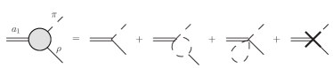
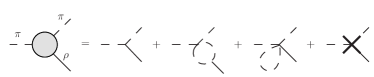
Figure 23: Diagrams depicting the $a\pi\rho$ and $\pi\pi\rho$ vertices expanded to 1-loop order; the cross represents counter-term contributions.

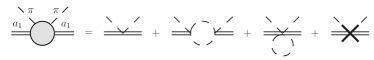
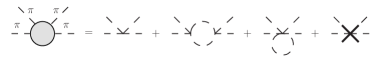
Figure 24: Diagrams depicting the $aa\pi\pi$ and $\pi\pi\pi\pi$ vertices expanded to 1-loop order; the cross represents counter-term contributions.

With the inclusion of the VCs the $\pi\rho$ loop in the self-energies $\Sigma_{a}^{L}$, $\Sigma_{a\pi}$, and $\Sigma_{\pi\pi}$ can be expressed as

$$\begin{split}\Sigma_{a}^{L(\pi\rho)}(p^{2})&=2i\int\limits_{0}^{\Lambda_{\rm cut}^{2}}\frac{-1}{\pi}\,dM^{2}\int\frac{d^{4}k}{(2\pi)^{4}}\,{\rm Im}\!\left[D_{\rho}(M^{2})V_{a}^{2}(M^{2})+\frac{1}{2}V_{aa}^{3\pi}(M^{2})\right]\frac{1}{k^{2}-M_{\pi}^{2}}\frac{1}{q^{2}-M^{2}}\left(-1+\frac{\left(p\cdot q\right)^{2}}{p^{2}M^{2}}\right)\ ,\\ \Sigma_{a\pi}^{(\pi\rho)}(p^{2})&=-2i\int\limits_{0}^{\Lambda_{\rm cut}^{2}}\frac{-1}{\pi}\,dM^{2}\int\frac{d^{4}k}{(2\pi)^{4}}\,{\rm Im}\!\left[D_{\rho}(M^{2})V_{a}(M^{2})V_{p}(M^{2})+\frac{1}{2}V_{ap}^{3\pi}(M^{2})\right]\frac{1}{k^{2}-M_{\pi}^{2}}\frac{1}{q^{2}-M^{2}}\left(-1+\frac{\left(p\cdot q\right)^{2}}{p^{2}M^{2}}\right),\\ \Sigma_{\pi\pi}^{(\pi\rho)}(p^{2})&=2i\int\limits_{0}^{\Lambda_{\rm cut}^{2}}\frac{-1}{\pi}\,dM^{2}\int\frac{d^{4}k}{(2\pi)^{4}}\,{\rm Im}\!\left[D_{\rho}(M^{2})V_{p}^{2}(M^{2})+\frac{1}{2}V_{pp}^{3\pi}(M^{2})\right]\frac{1}{k^{2}-M_{\pi}^{2}}\frac{1}{q^{2}-M^{2}}\left(-p^{2}+\frac{\left(p\cdot q\right)^{2}}{M^{2}}\right),\end{split}$$ (138)

where $q^{\mu}=p^{\mu}-k^{\mu}$, and a dispersion relation for the $\rho$ propagator has been used including the hard cut-off referred to in the main text. The 3-point vertices are represented by $V_{a}$ and $V_{p}$ and are decomposed into tree level and VC contributions as

$$\begin{split}V_{a}&=V_{a}^{\rm tree}+V_{a}^{VC},\\ V_{p}&=V_{p}^{\rm tree}+V_{p}^{VC},\end{split}$$ (139)

where

$$\begin{split}V_{a}^{\rm tree}(q^{2})&=\left(C+Fq^{2}\right),\\ V_{p}^{\rm tree}(q^{2})&=2\left(g_{\rho\pi\pi}+g_{\rho\pi\pi}^{(3)}q^{2}\right),\end{split}$$ (140)

for the non-linear realization, while the results for the linear version are found by replacing $C$ and $F$ with $\bar{C}$ and $\bar{F}$. These couplings are given by the equations in Appendix A. The 4-point vertices, $V^{3\pi}$, only have the VC contribution and are labeled by the external mesons.

In order to ensure that these expressions satisfy the relations of Eq. (29), the goal is to express the longitudinal self-energies as a coefficient times an integral which is the same between the different channels. Note that in the absence of the $\rho$ self-energy and the VCs this is obtainable and the PCAC relations are realized.

To compensate for the $\rho$ self-energy in the propagator, the VCs of the 3- and 4-point vertices need to be proportional to $\Sigma_{\rho}$. One can show that the $\pi\pi$ loop contribution to the VCs is related to the $\pi\pi$ loop of the $\rho$ self-energies, $\Sigma_{\rho}^{T(\pi\pi)}$, as

$$\begin{split}V_{a}^{VC(\pi\pi)}(q^{2})&=-\frac{3}{4}\frac{2\delta_{1}-\delta_{3}q^{2}}{g_{\rho\pi\pi}+g_{\rho\pi\pi}^{(3)}q^{2}}\Sigma_{\rho}^{T(\pi\pi)}(q^{2}),\\ V_{p}^{VC(\pi\pi)}(q^{2})&=-3\frac{2\gamma_{1}+\gamma_{2}q^{2}}{g_{\rho\pi\pi}+g_{\rho\pi\pi}^{(3)}q^{2}}\Sigma_{\rho}^{T(\pi\pi)}(q^{2}),\\ V_{aa}^{3\pi(\pi\pi)}(q^{2})&=\frac{9}{8}\left(\frac{2\delta_{1}-\delta_{3}q^{2}}{g_{\rho\pi\pi}+g_{\rho\pi\pi}^{(3)}q^{2}}\right)^{2}\Sigma_{\rho}^{T(\pi\pi)}(q^{2}),\\ V_{ap}^{3\pi(\pi\pi)}(q^{2})&=\frac{9}{2}\frac{(2\delta_{1}-\delta_{3}q^{2})(2\gamma_{1}+\gamma_{2}q^{2})}{(g_{\rho\pi\pi}+g_{\rho\pi\pi}^{(3)}q^{2})^{2}}\Sigma_{\rho}^{T(\pi\pi)}(q^{2}),\\ V_{pp}^{3\pi(\pi\pi)}(q^{2})&=18\left(\frac{2\gamma_{1}+\gamma_{2}q^{2}}{g_{\rho\pi\pi}+g_{\rho\pi\pi}^{(3)}q^{2}}\right)^{2}\Sigma_{\rho}^{T(\pi\pi)}(q^{2}),\end{split}$$ (141)

for the non-linear realization and

$$\begin{split}V_{a{\rm Lin}}^{VC(\pi\pi)}(q^{2})&=-\frac{1}{4}\frac{2\bar{\delta}_{1}-3\bar{\delta}_{3}q^{2}}{g_{\rho\pi\pi}+g_{\rho\pi\pi}^{(3)}q^{2}}\Sigma_{\rho}^{T(\pi\pi)}(q^{2}),\\ V_{p{\rm Lin}}^{VC(\pi\pi)}(q^{2})&=-\frac{2\bar{\gamma}_{1}+3\bar{\gamma}_{2}q^{2}}{g_{\rho\pi\pi}+g_{\rho\pi\pi}^{(3)}q^{2}}\Sigma_{\rho}^{T(\pi\pi)}(q^{2}),\\ V_{aa{\rm Lin}}^{3\pi(\pi\pi)}(q^{2})&=\frac{1}{8}\left(\frac{2\bar{\delta}_{1}-3\bar{\delta}_{3}q^{2}}{g_{\rho\pi\pi}+g_{\rho\pi\pi}^{(3)}q^{2}}\right)^{2}\Sigma_{\rho}^{T(\pi\pi)}(q^{2}),\\ V_{ap{\rm Lin}}^{3\pi(\pi\pi)}(q^{2})&=\frac{1}{2}\frac{(2\bar{\delta}_{1}-3\bar{\delta}_{3}q^{2})(2\bar{\gamma}_{1}+3\bar{\gamma}_{2}q^{2})}{(g_{\rho\pi\pi}+g_{\rho\pi\pi}^{(3)}q^{2})^{2}}\Sigma_{\rho}^{T(\pi\pi)}(q^{2}),\\ V_{pp{\rm Lin}}^{3\pi(\pi\pi)}(q^{2})&=2\left(\frac{2\bar{\gamma}_{1}+3\bar{\gamma}_{2}q^{2}}{g_{\rho\pi\pi}+g_{\rho\pi\pi}^{(3)}q^{2}}\right)^{2}\Sigma_{\rho}^{T(\pi\pi)}(q^{2}),\end{split}$$ (142)

for the linear realization. Again the couplings are as defined above. These results are then generalized to combine all contributions to the VCs through a $\rho$ self-energy which encompasses a $\pi\pi$ loop, a $\pi$ tadpole, and counter-term contributions, e.g.,

$$V_{a}^{VC}(q^{2})=-\frac{3}{4}\frac{2\delta_{1}-\delta_{3}q^{2}}{g_{\rho\pi\pi}+g_{\rho\pi\pi}^{(3)}q^{2}}\Sigma_{\rho}^{T}(q^{2}),$$ (143)

for the first expression in Eq. (141). This is obtained by choosing the appropriate couplings associated with the $\pi$ tadpole and counter-terms. The apparent energy dependence of the coupling will be justified a posteriori.

Using these relations between the VCs and $\Sigma_{\rho}^{T}$ allows for the expressions in Eq. (138) to be simplified. Furthermore, by choosing the coupling parameters to be

$$\begin{split}\delta_{1}&=-\frac{2g_{\rho\pi\pi}C}{3M_{\rho}^{2}},\quad\delta_{3}=\frac{4g_{\rho\pi\pi}^{(3)}C}{3M_{\rho}^{2}}\ ,\\ \gamma_{1}&=-\frac{g_{\rho\pi\pi}^{2}}{3M_{\rho}^{2}},\quad\gamma_{2}=-\frac{2g_{\rho\pi\pi}g_{\rho\pi\pi}^{(3)}}{3M_{\rho}^{2}}\ ,\\ \bar{\delta}_{1}&=-\frac{2g_{\rho\pi\pi}\bar{C}}{M_{\rho}^{2}},\quad\bar{\delta}_{3}=\frac{4g_{\rho\pi\pi}^{(3)}\bar{C}}{3M_{\rho}^{2}}\ ,\\ \bar{\gamma}_{1}&=-\frac{g_{\rho\pi\pi}^{2}}{M_{\rho}^{2}}\ ,\quad\bar{\gamma}_{2}=-\frac{2g_{\rho\pi\pi}g_{\rho\pi\pi}^{(3)}}{3M_{\rho}^{2}}\ ,\end{split}$$ (144)

which are different from their Lagrangian values, these expressions have the desired form of a coefficient times a generic integral. This integral is different from the case of a zero-width $\rho$, but it is still the same for the different channels. With these choices of parameters, we can also verify that Eq. (29) is satisfied, thus chiral symmetry is preserved. Returning to the proportionality factor between the VCs and $\Sigma_{\rho}^{T}$, we see that for the given choice of parameters in Eq. (144), this factor becomes energy independent which justifies the generalization that we postulated.

C.2 Transverse channel

For the transverse channel, $\Sigma_{a}^{T}$ has a more complicated form, given by

$$\begin{split}\Sigma_{a}^{T(\pi\rho)}(p^{2})&=2i\int-\frac{1}{\pi}dM^{2}\int\frac{d^{4}k}{(2\pi)^{4}}\left({\rm Im}\left[D_{\rho}(M^{2})(V_{a}^{T1}(M^{2}))^{2}+\frac{1}{2}V_{1}^{3\pi}(M^{2})\right]\frac{1}{k^{2}-M_{\pi}^{2}}\frac{1}{q^{2}-M^{2}}\right.\\ &+{\rm Im}\left[2D_{\rho}(M^{2})V_{a}^{T1}(M^{2})V_{a}^{T2}(M^{2})+\frac{1}{2}V_{2}^{3\pi}(M^{2})\right]\frac{p\cdot q}{k^{2}-M_{\pi}^{2}}\frac{1}{q^{2}-M^{2}}\\ &+{\rm Im}\left[D_{\rho}(M^{2})(V_{a}^{T2}(M^{2}))^{2}+\frac{1}{2}V_{3}^{3\pi}(M^{2})\right]\frac{(p\cdot q)^{2}}{k^{2}-M_{\pi}^{2}}\frac{1}{q^{2}-M^{2}}\\ &+{\rm Im}\left[D_{\rho}(M^{2})\left((V_{a}^{T1}(M^{2}))^{2}-(V_{a}^{T2}(M^{2}))^{2}p^{2}M^{2}\right)+\frac{1}{2}V_{4}^{3\pi}(M^{2})\right]\frac{1}{k^{2}-M_{\pi}^{2}}\frac{1}{q^{2}-M^{2}}\frac{1}{3M^{2}}\left(-q^{2}+\frac{(p\cdot q)^{2}}{p^{2}}\right)\Bigg{)}.\end{split}$$ (145)

where $q^{\mu}=p^{\mu}-k^{\mu}$. Note that when evaluating this integral using dimensional regulation, the 1/3 in the last term becomes a 1/($\delta$-1) where $\delta$ is the number of dimensions. The vertex functions, $V_{a}^{T1}$ and $V_{a}^{T2}$, can again be decomposed into a tree level part and a VC part as

$$\begin{split}V_{a}^{T1}&=V_{1}^{\rm tree}+V_{1}^{VC},\\ V_{a}^{T2}&=V_{2}^{\rm tree}+V_{2}^{VC}.\end{split}$$ (146)

The tree level terms are expressed as

$$\begin{split}V_{1}^{\rm tree}(q^{2})&=C-Ep^{2}+Fq^{2},\\ V_{2}^{\rm tree}(q^{2})&=2D+E-F,\end{split}$$ (147)

for the non-linear realization, with the expressions for the linear realization found by replacing $C$, $D$, $E$, and $F$ with $\bar{C}$, $\bar{D}$, $\bar{E}$, and $\bar{F}$. The functions $V^{3\pi}$ are associated with the $3\pi$ diagram’s contribution and are entirely a VC contribution.

To determine the functional form of the VCs, we utilize the same procedure as described above for the longitudinal channel of relating the VC loops to $\Sigma_{\rho}^{T}$ with the proportionality factor guided by the result from the $\pi\pi$ loop. To make the connection with chiral symmetry, we use the same values for the couplings, $\delta_{1}$, $\delta_{3}$, $\gamma_{1}$, $\gamma_{2}$ and the barred versions, as was determined in the longitudinal mode. Additionally, the transverse self-energy depends on the parameter $\delta_{2}$, which is not fixed by the previous considerations, but is chosen to be 0. This leads to the following expressions for the vertex functions in the non-linear realization,

$$\begin{split}V_{1}^{VC}(q^{2})&=-\frac{3}{4}\frac{2\delta_{1}-\delta_{3}q^{2}}{g_{\rho\pi\pi}+g_{\rho\pi\pi}^{(3)}q^{2}}\Sigma_{\rho}^{T}(q^{2}),\\ V_{2}^{VC}(q^{2})&=-\frac{3}{4}\frac{\delta_{3}}{g_{\rho\pi\pi}+g_{\rho\pi\pi}^{(3)}q^{2}}\Sigma_{\rho}^{T}(q^{2}),\\ V_{1}^{3\pi}(q^{2})&=\frac{9}{8}\left(\frac{2\delta_{1}-\delta_{3}q^{2}}{g_{\rho\pi\pi}+g_{\rho\pi\pi}^{(3)}q^{2}}\right)^{2}\Sigma_{\rho}^{T}(q^{2}),\\ V_{2}^{3\pi}(q^{2})&=\frac{9}{4}\frac{\left(2\delta_{1}-\delta_{3}q^{2}\right)\delta_{3}}{\left(g_{\rho\pi\pi}+g_{\rho\pi\pi}^{(3)}q^{2}\right)^{2}}\Sigma_{\rho}^{T}(q^{2}),\\ V_{3}^{3\pi}(q^{2})&=\frac{9}{8}\frac{\delta_{3}^{2}}{\left(g_{\rho\pi\pi}+g_{\rho\pi\pi}^{(3)}q^{2}\right)^{2}}\Sigma_{\rho}^{T}(q^{2}),\\ V_{4}^{3\pi}(q^{2})&=\frac{9}{8}\frac{\left(2\delta_{1}-\delta_{3}q^{2}\right)^{2}-\delta_{3}^{2}q^{2}p^{2}}{\left(g_{\rho\pi\pi}+g_{\rho\pi\pi}^{(3)}q^{2}\right)^{2}}\Sigma_{\rho}^{T}(q^{2}),\\ \end{split}$$ (148)

and in the linear realization,

$$\begin{split}V_{1{\rm Lin}}^{VC}(q^{2})&=-\frac{1}{4}\frac{2\bar{\delta}_{1}-3\bar{\delta}_{3}q^{2}}{g_{\rho\pi\pi}+g_{\rho\pi\pi}^{(3)}q^{2}}\Sigma_{\rho}^{T}(q^{2}),\\ V_{2{\rm Lin}}^{VC}(q^{2})&=-\frac{3}{4}\frac{\bar{\delta}_{3}}{g_{\rho\pi\pi}+g_{\rho\pi\pi}^{(3)}q^{2}}\Sigma_{\rho}^{T}(q^{2}),\\ V_{1{\rm Lin}}^{3\pi}(q^{2})&=\frac{1}{8}\left(\frac{2\bar{\delta}_{1}-3\bar{\delta}_{3}q^{2}}{g_{\rho\pi\pi}+g_{\rho\pi\pi}^{(3)}q^{2}}\right)^{2}\Sigma_{\rho}^{T}(q^{2}),\\ V_{2{\rm Lin}}^{3\pi}(q^{2})&=\frac{3}{4}\frac{\left(2\bar{\delta}_{1}-3\bar{\delta}_{3}q^{2}\right)\bar{\delta}_{3}}{\left(g_{\rho\pi\pi}+g_{\rho\pi\pi}^{(3)}q^{2}\right)^{2}}\Sigma_{\rho}^{T}(q^{2}),\\ V_{3{\rm Lin}}^{3\pi}(q^{2})&=\frac{9}{8}\frac{\bar{\delta}_{3}^{2}}{\left(g_{\rho\pi\pi}+g_{\rho\pi\pi}^{(3)}q^{2}\right)^{2}}\Sigma_{\rho}^{T}(q^{2}),\\ V_{4{\rm Lin}}^{3\pi}(q^{2})&=\frac{1}{8}\frac{\left(2\bar{\delta}_{1}-3\bar{\delta}_{3}q^{2}\right)^{2}-9\bar{\delta}_{3}^{2}q^{2}p^{2}}{\left(g_{\rho\pi\pi}+g_{\rho\pi\pi}^{(3)}q^{2}\right)^{2}}\Sigma_{\rho}^{T}(q^{2}).\\ \end{split}$$ (149)

Lastly, we note that the broad $\rho$ and VCs modify the $\rho\pi a_{1}$ coupling such that $\Sigma_{a}^{T}$ develops a mass shift at low temperatures of $\mathcal{O}(T^{2})$. To address this issue, we exploit the freedom associated with the partial resummation and the counter-terms, in particular those associated with $V_{2}^{VC}$. Choosing this term (rather than $V_{1}^{VC}$ which figures into the longitudinal channel, see first line of Eq. (141) or (142)) ensures that the following procedure does not affect the longitudinal mode which would disrupt the chiral relations in that channel. Because the divergence in the $\rho$ self-energy grows like $q^{6}$, the counter-terms have the general form of

$$V_{2}^{VC({\rm counter})}(q^{2})=A_{1}q^{2}+A_{2}q^{4}+A_{3}q^{6},$$ (150)

where the coefficients $A_{i}$ contain both the finite and infinite contributions of the counter-terms. Just as the nominal couplings are different from their Lagrangian values, so can the counter-terms. Therefore, we exploit this freedom and redefine $V_{2}^{VC}$ as

$$\begin{split}V_{2}^{VC}(q^{2})&=-\frac{3}{4}\frac{\delta_{3}}{g_{\rho\pi\pi}+g_{\rho\pi\pi}^{(3)}q^{2}}\Sigma_{\rho}^{T}(q^{2})+\eta_{1}q^{2}+\eta_{2}q^{4}+\eta_{3}q^{6},\\ V_{2{\rm Lin}}^{VC}(q^{2})&=-\frac{3}{4}\frac{\bar{\delta}_{3}}{g_{\rho\pi\pi}+g_{\rho\pi\pi}^{(3)}q^{2}}\Sigma_{\rho}^{T}(q^{2})+\bar{\eta}_{1}q^{2}+\bar{\eta}_{2}q^{4}+\bar{\eta}_{3}q^{6},\end{split}$$ (151)

where the finite contributions of the $A_{i}$’s are partitioned between a part which contributes to $\Sigma_{\rho}^{T}$ (making use of a derivative expansion for the fraction) and the $\eta_{i}$’s ($\bar{\eta}_{i}$’s). We determine $\eta_{1}$ ($\bar{\eta}_{1}$) by requiring that the low temperature real part of $\Sigma_{a}^{T}$ at an energy of $M_{a_{1}}$ is identical to the case without VCs and $\rho$ self-energies to recover the correct chiral behavior of no mass shift at ${\cal O}(T^{2})$. In principle, $\eta_{2}$ ($\bar{\eta}_{2}$) and $\eta_{3}$ ($\bar{\eta}_{3}$) are two additional parameters. However, at this point we only make use of adjusting $\eta_{2}$ ($\bar{\eta}_{2}$) and set $\eta_{3}$ ($\bar{\eta}_{3}$) to zero for simplicity. The parameter values are $\eta_{1}=1.51{\rm GeV}^{-1}$, $\eta_{2}=-1.805{\rm GeV}^{-3}$, $\eta_{3}=0$, $\bar{\eta}_{1}=1.108{\rm GeV}^{-1}$, $\bar{\eta}_{2}=-2.042{\rm GeV}^{-3}$, and $\bar{\eta}_{3}=0$.

Appendix D Loop integrals for finite temperature self-energy calculation

In this section, we present the loop integrals to be evaluated for the finite temperature calculations of the self-energies. In each case, we have already performed the sum over Matsubara frequencies. Terms which are not proportional to a thermal Bose factor are associated with vacuum contributions.

The self-energy of a $h\to h_{1}h_{2}\to h$ loop diagram has the generic form

$$\begin{split}&\Sigma(p_{0},|\vec{p}|)=\int\frac{d^{3}k}{(2\pi)^{3}}\frac{1}{4E_{h_{1}}(\vec{k})E_{h_{2}}(\vec{p}-\vec{k})}\\ &\times\left(\frac{1}{p_{0}-E_{h_{1}}(\vec{k})-E_{h_{2}}(\vec{p}-\vec{k})+i\epsilon}\left[\left(\frac{1}{2}+f^{B}(E_{h_{1}}(\vec{k}))\right){\cal V}(E_{h_{1}}(\vec{k}))+\left(\frac{1}{2}+f^{B}(E_{h_{2}}(\vec{p}-\vec{k}))\right){\cal V}(p_{0}-E_{h_{2}}(\vec{p}-\vec{k}))\right]\right.\\ &+\frac{1}{p_{0}+E_{h_{1}}(\vec{k})-E_{h_{2}}(\vec{p}-\vec{k})+i\epsilon}\left[\left(\frac{1}{2}+f^{B}(E_{h_{1}}(\vec{k}))\right){\cal V}(-E_{h_{1}}(\vec{k}))-\left(\frac{1}{2}+f^{B}(E_{h_{2}}(\vec{p}-\vec{k}))\right){\cal V}(p_{0}-E_{h_{2}}(\vec{p}-\vec{k}))\right]\\ &-\frac{1}{p_{0}-E_{h_{1}}(\vec{k})+E_{h_{2}}(\vec{p}-\vec{k})+i\epsilon}\left[\left(\frac{1}{2}+f^{B}(E_{h_{1}}(\vec{k})\right){\cal V}(E_{h_{1}}(\vec{k}))-\left(\frac{1}{2}+f^{B}(E_{h_{2}}(\vec{p}-\vec{k}))\right){\cal V}(p_{0}+E_{h_{2}}(\vec{p}-\vec{k}))\right]\\ &\left.-\frac{1}{p_{0}+E_{h_{1}}(\vec{k})+E_{h_{2}}(\vec{p}-\vec{k})+i\epsilon}\left[\left(\frac{1}{2}+f^{B}(E_{h_{1}}(\vec{k}))\right){\cal V}(-E_{h_{1}}(\vec{k}))+\left(\frac{1}{2}+f^{B}(E_{h_{2}}(\vec{p}-\vec{k}))\right){\cal V}(p_{0}+E_{h_{2}}(\vec{p}-\vec{k}))\right]\right).\end{split}$$ (152)

Throughout, we use the notation $E_{h}(\vec{k})=(|\vec{k}|^{2}+M_{h}^{2})^{1/2}$ for the on-shell energies of hadron $h$. In the integral, $h_{1}$ and $h_{2}$ are determined by the diagram in question, and will be specified for each case below. The Bose distributions are given by $f^{B}(E)=(e^{E/T}-1)^{-1}$. The function ${\cal V}(E)$ is related to the vertices and is unique for each diagram; it generically depends on combinations of $p_{0}$, $\vec{p}$, and $\vec{k}$, while its dependence on an energy argument is specified in the expression above and in the following ones. In the self-energy, Eq. (152), the first term is associated with the decay process (or unitarity cut) including final-state Bose enhancement. The second and third terms are associated with scattering processes (or Landau cuts) where the thermal mesons are $h_{1}$ and $h_{2}$, respectively. The fourth term is the unitarity cut for negative energies, ensuring the retarded property of the self-energy.

The tadpole diagrams are completely real and have a simpler structure and will be quoted in due course.

D.1 Vector channel

We begin with the $\rho$ self-energy. At finite temperature, we consider the case of finite 3-momentum, inducing different 3D-transverse, $\Sigma_{\rho}^{\perp}$, and -longitudinal, $\Sigma_{\rho}^{\parallel}$, self-energies. For the non-linear realization, each of these self-energies is comprised of three diagrams: the $\pi\pi$ loop (first diagram of the top row in Fig. 3), the $\pi$-tadpole (second diagram of the top row in Fig. 3), and the $\pi a_{1}$ loop (diagram in in Fig. 11). The linear realization allows for three new diagrams because of the explicit $\sigma$ field: a $\sigma$ tadpole (first diagram in Fig. 4), a $\sigma\rho$ loop (second diagram in Fig. 4), and a lollipop diagram (first diagram in Fig. 11).

For the $\pi\pi$ loop, the self-energy is in the form of Eq. (152) with $M_{h_{1}}=M_{h_{2}}=M_{\pi}$. For $\Sigma_{\rho}^{\perp}$, the vertex function reads

$${\cal V}_{\perp}^{(\pi\pi)}(k_{0})=2\left(g_{\rho\pi\pi}+g_{\rho\pi\pi}^{(3)}p^{2}\right)^{2}|\vec{k}|^{2}(1-x^{2})$$ (153)

while for $\Sigma_{\rho}^{\parallel}$ it is given by

$$\begin{split}{\cal V}_{\parallel}^{(\pi\pi)}(k_{0})&=4\left(g_{\rho\pi\pi}+g_{\rho\pi\pi}^{(3)}p^{2}\right)^{2}\\ &\times\left(-k_{0}^{2}+|\vec{k}|^{2}x^{2}+\frac{(p\cdot k)^{2}}{p^{2}}\right)\ .\end{split}$$ (154)

In these expressions, $p^{2}=p_{0}^{2}-|\vec{p}|^{2}$, $k^{2}=k_{0}^{2}-|\vec{k}|^{2}$, $p\cdot k=p_{0}k_{0}-\vec{p}\cdot\vec{k}$, and $x=\cos(\theta)$ with $\theta$ being the angle between $\vec{p}$ and $\vec{k}$. We will use this notation throughout this section. The above two contributions are identicl for the two realizations.

For the $\pi$ tadpole the two self-energies in the non-linear realization are

$$\begin{split}\Sigma_{\rho}^{\perp(\pi{\rm Tad})}(p_{0},|\vec{p}|)&=-2\int\frac{d^{3}k}{(2\pi)^{3}}\frac{1+2f^{B}(E_{\pi}(\vec{k}))}{E_{\pi}(\vec{k})}\left[\alpha_{1}+2\alpha_{2}p^{2}-\alpha_{8}\left(M_{\pi}^{2}+\frac{1}{2}\left(|\vec{k}|^{2}-\frac{(\vec{p}\cdot\vec{k})^{2}}{|\vec{p}|^{2}}\right)\right)\right],\\ \Sigma_{\rho}^{\parallel(\pi{\rm Tad})}(p_{0},|\vec{p}|)&=-2\int\frac{d^{3}k}{(2\pi)^{3}}\frac{1+2f^{B}(E_{\pi}(\vec{k}))}{E_{\pi}(\vec{k})}\left[\alpha_{1}+2\alpha_{2}p^{2}-\alpha_{8}\left(\frac{p_{0}^{2}E_{\pi}(\vec{k})^{2}}{p^{2}}+\left(\vec{p}\cdot\vec{k}\right)^{2}\left(\frac{1}{p^{2}}+\frac{1}{|\vec{p}|^{2}}\right)-|\vec{k}|^{2}\right)\right],\end{split}$$ (155)

and for the linear realization

$$\begin{split}\Sigma_{\rho{\rm Lin}}^{\perp(\pi{\rm Tad})}(p_{0},|\vec{p}|)&=-2\int\frac{d^{3}k}{(2\pi)^{3}}\frac{1+2f^{B}(E_{\pi}(\vec{k}))}{E_{\pi}(\vec{k})}\left[\bar{\alpha}_{1}+\bar{\alpha}_{2}p^{2}-\bar{\alpha}_{8}\left(M_{\pi}^{2}+\frac{1}{2}\left(|\vec{k}|^{2}-\frac{(\vec{p}\cdot\vec{k})^{2}}{|\vec{p}|^{2}}\right)\right)\right],\\ \Sigma_{\rho{\rm Lin}}^{\parallel(\pi{\rm Tad})}(p_{0},|\vec{p}|)&=-2\int\frac{d^{3}k}{(2\pi)^{3}}\frac{1+2f^{B}(E_{\pi}(\vec{k}))}{E_{\pi}(\vec{k})}\left[\bar{\alpha}_{1}+\bar{\alpha}_{2}p^{2}-\bar{\alpha}_{8}\left(\frac{p_{0}^{2}E_{\pi}(\vec{k})^{2}}{p^{2}}+\left(\vec{p}\cdot\vec{k}\right)^{2}\left(\frac{1}{p^{2}}+\frac{1}{|\vec{p}|^{2}}\right)-|\vec{k}|^{2}\right)\right].\end{split}$$ (156)

For the $\pi a_{1}$ loop, the self-energy is of the form in Eq. (152) with $M_{h_{1}}=M_{\pi}$ and $M_{h_{2}}=M_{a_{1}}$. For $\Sigma_{\rho}^{\perp}$, the 3D-transverse vertex function is given by

$$\begin{split}{\cal V}_{\perp}^{(\pi a_{1})}(k_{0})&=2\left(C-(2D-E-F)p\cdot k+2Dp^{2}-Ek^{2}\right)^{2}+(1-x^{2})\frac{|\vec{k}|^{2}}{M_{a_{1}}^{2}}\\ &\times\left(p^{2}(2CF-M_{a_{1}}^{2}(4D(D+E-F)+F^{2})+F^{2}p^{2})+E^{2}M_{a_{1}}^{2}(k^{2}-2p\cdot k-M_{a_{1}}^{2})\right),\end{split}$$ (157)

and for the 3D-longitudinal part

$$\begin{split}{\cal V}_{\parallel}^{(\pi a_{1})}(k_{0})&=2\left(C-(2D-E-F)p\cdot k+2Dp^{2}-Ek^{2}\right)^{2}+\frac{1}{M_{a_{1}}^{2}}\left(-k_{0}^{2}+|\vec{k}|^{2}x^{2}+\frac{(p\cdot k)^{2}}{p^{2}}\right)\\ &\times\left(p^{2}(2CF-M_{a_{1}}^{2}(4D(D+E-F)+F^{2})+F^{2}p^{2})+E^{2}M_{a_{1}}^{2}(k^{2}-2p\cdot k-M_{a_{1}}^{2})\right)\end{split}$$ (158)

For the linear realization ${\cal V}_{\perp}$ and ${\cal V}_{\parallel}$ are identical but with the couplings $C$, $D$, $E$, $F$ replaced by $\bar{C}$, $\bar{D}$, $\bar{E}$, $\bar{F}$.

The $\sigma$ tadpole provides the same contribution to both the 3D-transverse and -longitudinal self-energies and is given by

$$\Sigma_{\rho{\rm Lin}}^{\perp/\parallel(\sigma{\rm Tad})}(p_{0},|\vec{p}|)=e_{1}p^{2}\int\frac{d^{3}k}{(2\pi)^{3}}\frac{1+2f^{B}(E_{\sigma}(\vec{k}))}{E_{\sigma}(\vec{k})}.$$ (159)

The $\sigma\rho$ loop contribution has the form of Eq. (152) with $M_{h_{1}}=M_{\sigma}$ and $M_{h_{2}}=M_{\rho}$. The functions ${\cal V}$ for the two polarizations are:

$$\begin{split}{\cal V}_{\perp{\rm Lin}}^{(\sigma\rho)}(k_{0})&=(4c_{1})^{2}\left[\left(p^{2}-p\cdot k\right)^{2}-\frac{1}{2}p^{2}|k|^{2}(1-x^{2})\right],\\ {\cal V}_{\parallel{\rm Lin}}^{(\sigma\rho)}(k_{0})&=(4c_{1})^{2}\left[\left(p^{2}-p\cdot k\right)^{2}-p^{2}\left(-k_{0}^{2}+\frac{(p\cdot k)^{2}}{p^{2}}+\frac{(\vec{p}\cdot\vec{k})^{2}}{|\vec{p}|^{2}}\right)\right].\end{split}$$ (160)

Finally, for the $\rho$ self-energy, the contribution from the lollipop diagrams is identical for the two polarizations,

$$\Sigma_{\rho{\rm Lin}}^{\perp/\parallel({\rm lolli})}(p_{0},|\vec{p}|)=\frac{4c_{1}p^{2}}{M_{\sigma}^{2}}\left(\Sigma_{\rm lolli}^{\pi}+\Sigma_{\rm lolli}^{\sigma}\right)\ .$$ (161)

The terms $\Sigma_{\rm lolli}^{\pi}$ and $\Sigma_{\rm lolli}^{\sigma}$ are associated with the pion and sigma loops in the diagram of Fig. 11 and read

$$\begin{split}\Sigma_{\rm lolli}^{\pi}&=-Z_{\pi}\sigma_{0}\left(\lambda+\frac{g_{\rho\pi\pi}^{2}M_{\pi}^{2}}{M_{\rho}^{2}Z_{\pi}^{2}}\right)\\ &\times\int\frac{d^{3}k}{(2\pi)^{3}}\frac{1+2f^{B}(E_{\pi}(\vec{k}))}{2E_{\pi}(\vec{k})},\\ \Sigma_{\rm lolli}^{\sigma}&=-3\lambda\sigma_{0}\int\frac{d^{3}k}{(2\pi)^{3}}\frac{1+2f^{B}(E_{\sigma}(\vec{k}))}{2E_{\sigma}(\vec{k})}.\end{split}$$ (162)

D.2 Axial-vector channel

In the $AV$ and pion channels, there are four self-energies, the $a_{1}$ self-energy for the 4D-transverse and -longitudinal channels ($\Sigma_{a_{1}}^{T}$ and $\Sigma_{a_{1}}^{L}$) the pion self-energy ($\Sigma_{\pi\pi}$), and the $a_{1}-\pi$ transition self-energy ($\Sigma_{a\pi}$). Each self-energy has two contributions in both realizations, a $\pi\rho$ loop and a $\pi$-tadpole, as shown in the bottom row of Fig. 3, and an additional four contributions which are unique to the linear realization, a $\pi\sigma$ loop, a $\sigma$ tadpole, a $\sigma a_{1}$ loop, and a lollipop diagram (cf. the last three diagrams in Fig. 4 and Fig. 11, all with appropriate external legs). In this paper, only the zero-momentum case is analyzed for these self-energies. Thus expressions will be presented only for this case.

The $\pi\rho$ loop within the $AV$ channel is more involved than the expressions already presented because of the resummed $\rho$ propagator and associated VCs, which involve an additional integral. Because we are concerned only with the vacuum broadening of the $\rho$ meson and the vacuum VCs, this additional integral is only over the invariant mass of the $\rho$ meson.

The transverse $a_{1}$ self-energy can be written in the form

$$\begin{split}\Sigma_{a_{1}}^{T(\pi\rho)}(p_{0})&=\int\limits_{0}^{\Lambda_{\rm cut}^{2}}\frac{-1}{\pi}dM^{2}\left({\rm Im}\left[D_{\rho}(M^{2})\right]\tilde{\Sigma}_{1}(p_{0})\right.\\ &\left.+{\rm Im}\left[D_{\rho}(M^{2})\left(\left(V_{a}^{T1}(M^{2})\right)^{2}-(V_{a}^{T2}(M^{2}))^{2}p_{0}^{2}M^{2}\right)+\frac{1}{2}V_{4}^{3\pi}(M^{2})\right]\frac{1}{3}\tilde{\Sigma}_{2}(p_{0})\right),\end{split}$$ (163)

where the integration is over the invariant mass of the resummed $\rho$ meson. The vertex functions, $V_{a}^{T1}$, $V_{a}^{T2}$, and the $V_{i}^{3\pi}$s, are evaluated in the vacuum (specific to the realization) and have been quoted in the previous section. The temperature dependence of the integral in Eq. (163) resides in the functions $\tilde{\Sigma}_{1}$ and $\tilde{\Sigma}_{2}$. They are of the form of Eq. (152) with $M_{h_{1}}=M_{\pi}$ and $M_{h_{2}}=M$ (the $\rho$’s invariant mass) and vertex functions

$$\begin{split}{\cal V}_{1}(k_{0})&=2\left[\left(V_{a}^{T1}(q^{2})+p_{0}(p_{0}-k_{0})V_{a}^{T2}(q^{2})\right)^{2}+\frac{1}{2}D_{\rho}^{-1}(q^{2})\left(V_{1}^{3\pi}(q^{2})+p_{0}(p_{0}-k_{0})V_{2}^{3\pi}+p_{0}^{2}(p_{0}-k_{0})^{2}V_{3}^{3\pi}\right)\right]\end{split}$$ (164)

for the former (with $q^{2}=(p_{0}-k_{0})^{2}-|\vec{k}|^{2}$) and ${\cal V}_{2}(k_{0})=2|\vec{k}|^{2}/M^{2}$ for the latter. Additionally, to preserve the retarded properties of the self-energy and because we have integrate over $M^{2}$, the calculation of $\tilde{\Sigma}_{1}$ requires using the complex conjugate, ${\cal V}_{1}^{*}(p_{0}+E_{h_{2}})$. The VC loop integrals are again the same as presented in the previous section.

For $\Sigma_{a_{1}}^{L}$, $\Sigma_{a\pi}$ and $\Sigma_{\pi\pi}$, the $\pi\rho$ loop contribution (in both realizations) has the form

$$\begin{split}\Sigma_{a}^{L(\pi\rho)}(p_{0})&=\int\limits_{0}^{\Lambda_{\rm cut}^{2}}\frac{-1}{\pi}\,dM^{2}{\rm Im}\!\left[D_{\rho}(M^{2})V_{a}^{2}(M^{2})+\frac{1}{2}V_{aa}^{3\pi}(M^{2})\right]\tilde{\Sigma}_{2}(p_{0}),\\ \Sigma_{a\pi}^{(\pi\rho)}(p_{0})&=-\int\limits_{0}^{\Lambda_{\rm cut}^{2}}\frac{-1}{\pi}\,dM^{2}{\rm Im}\!\left[D_{\rho}(M^{2})V_{a}(M^{2})V_{p}(M^{2})+\frac{1}{2}V_{ap}^{3\pi}(M^{2})\right]\tilde{\Sigma}_{2}(p_{0}),\\ \Sigma_{\pi\pi}^{(\pi\rho)}(p_{0})&=\int\limits_{0}^{\Lambda_{\rm cut}^{2}}\frac{-1}{\pi}\,dM^{2}{\rm Im}\!\left[D_{\rho}(M^{2})V_{p}^{2}(M^{2})+\frac{1}{2}V_{pp}^{3\pi}(M^{2})\right]\tilde{\Sigma}_{2}(p_{0}),\end{split}$$ (165)

where the integration is over the invariant mass of the dressed $\rho$ meson. This is similar to the vacuum structure of Eq. (138). The function $\tilde{\Sigma}_{2}$ is the same as described above, encoding the temperature dependence. The pertinent vertex functions for each realization are given by their vacuum forms as presented in the previous section.

For the longitudinal self-energies, the $\pi\rho$ loop also has an additional term which is completely real and thereby cannot be expressed in a form similar to the above expressions. These extra terms are

$$\begin{split}\Sigma_{a_{1}}^{L({\rm extra})}(p_{0})&=\frac{C^{2}}{M_{\rho}^{2}}\int\frac{d^{3}k}{(2\pi)^{3}}\frac{1+2f^{B}(E_{\pi}(\vec{k}))}{E_{\pi}(\vec{k})},\\ \Sigma_{a\pi}^{({\rm extra})}(p_{0})&=-\frac{g_{\rho\pi\pi}C}{M_{\rho}^{2}}\int\frac{d^{3}k}{(2\pi)^{3}}\frac{1+2f^{B}(E_{\pi}(\vec{k}))}{E_{\pi}(\vec{k})},\\ \Sigma_{\pi\pi}^{({\rm extra})}(p_{0})&=\frac{g_{\rho\pi\pi}^{2}}{M_{\rho}^{2}}\left(p_{0}^{2}+M_{\pi}^{2}\right)\int\frac{d^{3}k}{(2\pi)^{3}}\frac{1+2f^{B}(E_{\pi}(\vec{k}))}{E_{\pi}(\vec{k})}\ .\end{split}$$ (166)

They are the same in the linear realization except for replacing $C$ by $\bar{C}$.

The pion tadpole contributions in the non-linear realization are as follows:

$$\begin{split}\Sigma_{a_{1}}^{T(\pi{\rm Tad})}(p_{0})&=-2\int\frac{d^{3}k}{(2\pi)^{3}}\frac{1+2f^{B}(E_{\pi}(\vec{k}))}{E_{\pi}(\vec{k})}\left(\beta_{1}+2\beta_{2}p_{0}^{2}-\beta_{7}\left(M_{\pi}^{2}+\frac{1}{3}|\vec{k}|^{2}\right)\right),\\ \Sigma_{a_{1}}^{L(\pi{\rm Tad})}(p_{0})&=2\int\frac{d^{3}k}{(2\pi)^{3}}\frac{1+2f^{B}(E_{\pi}(\vec{k}))}{E_{\pi}(\vec{k})}\left(\beta_{1}+\beta_{7}|\vec{k}|^{2}\right),\\ \Sigma_{a\pi}^{(\pi{\rm Tad})}(p_{0})&=-\int\frac{d^{3}k}{(2\pi)^{3}}\frac{1+2f^{B}(E_{\pi}(\vec{k}))}{E_{\pi}(\vec{k})}\left(\delta_{1}+\delta_{3}|\vec{k}|^{2}\right),\\ \Sigma_{\pi\pi}^{(\pi{\rm Tad})}(p_{0})&=2\int\frac{d^{3}k}{(2\pi)^{3}}\frac{1+2f^{B}(E_{\pi}(\vec{k}))}{E_{\pi}(\vec{k})}\left(\gamma_{1}(p_{0}^{2}+M_{\pi}^{2})-2\gamma_{2}p_{0}^{2}|\vec{k}|^{2}-5\gamma_{3}\right)\ ,\end{split}$$ (167)

and in the linear realization

$$\begin{split}\Sigma_{a_{1}{\rm Lin}}^{T(\pi{\rm Tad})}(p_{0})&=\int\frac{d^{3}k}{(2\pi)^{3}}\frac{1+2f^{B}(E_{\pi}(\vec{k}))}{E_{\pi}(\vec{k})}\left(\bar{\beta}_{1}-2\bar{\beta_{2}}p_{0}^{2}+2\bar{\beta}_{7}\left(M_{\pi}^{2}+\frac{1}{3}|\vec{k}|^{2}\right)\right),\\ \Sigma_{a_{1}{\rm Lin}}^{L(\pi{\rm Tad})}(p_{0})&=-\int\frac{d^{3}k}{(2\pi)^{3}}\frac{1+2f^{B}(E_{\pi}(\vec{k}))}{E_{\pi}(\vec{k})}\left(\bar{\beta}_{1}-2\bar{\beta}_{7}|\vec{k}|^{2}\right),\\ \Sigma_{a\pi{\rm Lin}}^{(\pi{\rm Tad})}(p_{0})&=\frac{1}{2}\int\frac{d^{3}k}{(2\pi)^{3}}\frac{1+2f^{B}(E_{\pi}(\vec{k}))}{E_{\pi}(\vec{k})}\left(\bar{\delta}_{1}-2\bar{\delta}_{3}|\vec{k}|^{2}\right),\\ \Sigma_{\pi\pi{\rm Lin}}^{(\pi{\rm Tad})}(p_{0})&=-\int\frac{d^{3}k}{(2\pi)^{3}}\frac{1+2f^{B}(E_{\pi}(\vec{k}))}{E_{\pi}(\vec{k})}\left(\bar{\gamma}_{1}(p_{0}^{2}+M_{\pi}^{2})+4\bar{\gamma}_{2}p_{0}^{2}|\vec{k}|^{2}+10\bar{\gamma}_{3}\right)\ .\end{split}$$ (168)

For the $\sigma$ tadpole, the self-energies are given by

$$\begin{split}\Sigma_{a_{1}{\rm Lin}}^{T(\sigma{\rm Tad})}(p_{0})&=\left(f_{1}+2f_{2}p_{0}^{2}\right)\int\frac{d^{3}k}{(2\pi)^{3}}\frac{1+2f^{B}(E_{\sigma}(\vec{k}))}{E_{\sigma}},\\ \Sigma_{a_{1}{\rm Lin}}^{L(\sigma{\rm Tad})}(p_{0})&=-f_{1}\int\frac{d^{3}k}{(2\pi)^{3}}\frac{1+2f^{B}(E_{\sigma}(\vec{k}))}{E_{\sigma}},\\ \Sigma_{a\pi{\rm Lin}}^{(\sigma{\rm Tad})}(p_{0})&=\frac{g_{1}}{2}\int\frac{d^{3}k}{(2\pi)^{3}}\frac{1+2f^{B}(E_{\sigma}(\vec{k}))}{E_{\sigma}},\\ \Sigma_{\pi\pi{\rm Lin}}^{(\sigma{\rm Tad})}(p_{0})&=-(h_{1}+h_{2}p_{0}^{2})\int\frac{d^{3}k}{(2\pi)^{3}}\frac{1+2f^{B}(E_{\sigma}(\vec{k}))}{E_{\sigma}}\ .\end{split}$$ (169)

The $\pi\sigma$ loop has the structure of Eq. (152) with $M_{h_{1}}=M_{\pi}$ and $M_{h_{2}}=M_{\sigma}$ and vertex functions

$$\begin{split}{\cal V}_{a_{1}{\rm Lin}}^{T(\pi\sigma)}(k_{0})&=\frac{1}{3}|\vec{k}|^{2}\left(b_{1}-b_{2}-b_{3}p_{0}^{2}\right)^{2},\\ {\cal V}_{a_{1}{\rm Lin}}^{L(\pi\sigma)}(k_{0})&=\left(b_{1}p_{0}+k_{0}(b_{2}-b_{1})\right)^{2},\\ {\cal V}_{a\pi{\rm Lin}}^{(\pi\sigma)}(k_{0})&=-\frac{1}{p_{0}^{2}}\left(b_{1}p_{0}^{2}-\left(b_{1}-b_{2}\right)p_{0}k_{0}\right)\left(2a_{1}+2\left(a_{2}-a_{3}\right)k_{0}p_{0}+a_{3}\left(k^{2}+p_{0}^{2}\right)\right),\\ {\cal V}_{\pi\pi{\rm Lin}}^{(\pi\sigma)}(k_{0})&=\left(2a_{1}+2a_{2}p_{0}k_{0}+a_{3}(p_{0}^{2}-2p_{0}k_{0}+k^{2})\right)^{2}.\end{split}$$ (170)

The $\sigma a_{1}$ loop has the structure given in Eq. (152) with $M_{h_{1}}=M_{\sigma}$, $M_{h_{2}}=M_{a_{1}}$ and vertex functions for each channel defined as:

$$\begin{split}{\cal V}_{a_{1}{\rm Lin}}^{T(\sigma a_{1})}(k_{0})&=\left(2d_{1}+d_{3}k^{2}-4d_{2}k_{0}p_{0}+4d_{2}p_{0}^{2}\right)^{2}\\ &+\frac{1}{3}\frac{|\vec{k}|^{2}}{M_{a_{1}}^{2}}\left(4d_{1}^{2}+4d_{1}d_{3}(M_{a_{1}}^{2}+p_{0}^{2})+d_{3}^{2}(k^{2}M_{a_{1}}^{2}-2M_{a_{1}}^{2}k_{0}p_{0}-M_{a_{1}}^{2}p_{0}^{2}+p_{0}^{4})+16d_{2}p_{0}^{2}M_{a_{1}}^{2}(d_{3}-d_{2})\right),\\ {\cal V}_{a_{1}{\rm Lin}}^{L(\sigma a_{1})}(k_{0})&=-\left(2d_{1}+d_{3}(p_{0}^{2}-2p_{0}k_{0}+k^{2})\right)^{2}\\ &-\frac{p_{0}-k_{0}}{p_{0}M_{a_{1}}^{2}}\left(4d_{1}^{2}+4d_{1}d_{3}M_{a_{1}}^{2}+d_{3}^{2}M_{a_{1}}^{2}(p_{0}^{2}-2p_{0}k_{0}+k^{2})\right),\\ {\cal V}_{a\pi{\rm Lin}}^{(\sigma a_{1})}(k_{0})&=-\frac{1}{M_{a_{1}}^{2}p_{0}^{2}}\left(2d_{1}\left(b_{1}\left(k^{2}p_{0}^{2}+k_{0}^{2}p_{0}^{2}-k_{0}p_{0}(k^{2}-M_{a_{1}}^{2}+p_{0}^{2})\right)+b_{2}(k_{0}^{2}p_{0}^{2}-2k_{0}p_{0}^{3}-M_{a_{1}}^{2}p_{0}^{2}+p_{0}^{4})+b_{3}M_{a_{1}}^{2}p_{0}^{2}|\vec{k}|^{2}\right)\right.\\ &\left.+d_{3}M_{a_{1}}^{2}p_{0}^{2}|\vec{k}|^{2}\left(b_{2}-b_{1}+b_{3}(k^{2}-2k_{0}p_{0}+p_{0}^{2})\right)\right),\\ {\cal V}_{\pi\pi{\rm Lin}}^{(\sigma a_{1})}(k_{0})&=(b_{1}-b_{2}-b_{3}(p_{0}^{2}-2p_{0}k_{0}+k^{2}))^{2}\left(-p_{0}^{2}+\frac{(p_{0}^{2}-p_{0}k_{0})^{2}}{M_{a_{1}}^{2}}\right)\\ &+\frac{1}{M_{a_{1}}^{2}}\left(p_{0}^{2}-2p_{0}k_{0}+k^{2}-M_{a_{1}}^{2}\right)\Big{(}2(b_{1}-b_{2}-b_{3}(p_{0}^{2}-2p_{0}k_{0}+k^{2}))(b_{3}(p_{0}^{2}-p_{0}k_{0})-b1)(p_{0}^{2}-p_{0}k_{0})\\ &\left.+\left(b_{3}(p_{0}^{2}-p_{0}k_{0})-b_{1}\right)^{2}(p_{0}^{2}-2p_{0}k_{0}+k^{2})\right).\end{split}$$ (171)

The last contributions are the lollipop diagrams which read

$$\begin{split}\Sigma_{a_{1}{\rm Lin}}^{T({\rm Lolli})}(p_{0})&=\left(2d_{1}+4d_{2}p_{0}^{2}\right)\frac{1}{M_{\sigma}^{2}}\left(\Sigma_{\rm lolli}^{\pi}+\Sigma_{\rm lolli}^{\sigma}\right),\\ \Sigma_{a_{1}{\rm Lin}}^{L({\rm Lolli})}(p_{0})&=\frac{2d_{1}}{M_{\sigma}^{2}}\left(\Sigma_{\rm lolli}^{\pi}+\Sigma_{\rm lolli}^{\sigma}\right),\\ \Sigma_{a\pi{\rm Lin}}^{({\rm Lolli})}(p_{0})&=\frac{b_{2}}{M_{\sigma}^{2}}\left(\Sigma_{\rm lolli}^{\pi}+\Sigma_{\rm lolli}^{\sigma}\right),\\ \Sigma_{\pi\pi{\rm Lin}}^{({\rm Lolli})}(p_{0})&=\frac{-2(a_{1}+a_{2}p_{0}^{2})}{M_{\sigma}^{2}}\left(\Sigma_{\rm lolli}^{\pi}+\Sigma_{\rm lolli}^{\sigma}\right).\end{split}$$ (172)

References

- (1) S. Borsanyi et al. [Wuppertal-Budapest Collaboration], JHEP 1009, 073 (2010).
- (2) A. Bazavov et al., Phys. Rev. D 85 054503 (2012).
- (3) R. J. Porter et al. [DLS Collaboration], Phys. Rev. Lett. 79, 1229 (1997).
- (4) D. Adamova et al. [CERES/NA45 Collaboration] Phys. Lett. B 666, 425 (2008).
- (5) R. Arnaldi et al. [NA60 Collaboration], Eur. Phys. J. C 61, 711 (2009).
- (6) G. Agakishiev et al. [HADES Collaboration], Phys. Rev. C 84, 014902 (2011).
- (7) F. Geurts [STAR Collaboration], Nucl. Phys. A 904-905, 217c (2013).
- (8) R. Rapp, J. Wambach and H. van Hees, in Relativistic Heavy-Ion Physics, edited by R. Stock and Landolt Börnstein (Springer, Berlin, 2010), New Series I/23A, p. 4-1; [arXiv:0901.3289 [hep-ph]].
- (9) R. Rapp, Adv. High Energy Phys. 2013, 148253 (2013).
- (10) P. M. Hohler and R. Rapp, Phys. Lett. B 731, 103 (2014).
- (11) A. Ayala, C. A. Dominguez, M. Loewe and Y. Zhang, Phys. Rev. D 90, 034012 (2014).
- (12) C.-N. Yang and R.L. Mills, Phys. Rev. 96, 191 (1954).
- (13) J. Gasser and H. Leutwyler, Annals Phys. 158, 142 (1984).
- (14) H. Gomm, O. Kaymakcalan and J. Schechter, Phys. Rev. D 30, 2345 (1984).
- (15) M. Bando, T. Kugo and K. Yamawaki, Phys. Rept. 164, 217 (1988).
- (16) M. Harada and K. Yamawaki, Phys. Rept. 381, 1 (2003).
- (17) C. Song, Phys. Rev. C 47, 2861 (1993).
- (18) P. Ko and S. Rudaz, Phys. Rev. D 50, 6877 (1994).
- (19) C. Song, Phys. Rev. D 48, 1375 (1993).
- (20) C. Song, Phys. Rev. D 49, 1556 (1994).
- (21) R. D. Pisarski, Phys. Rev. D 52, 3773 (1995); Nucl. Phys. A 590, 553C (1995); hep-ph/9503330.
- (22) R. Barate et al. [ALEPH Collaboration], Eur. Phys. J. C 4, 409 (1998).
- (23) K. Ackerstaff et al. [OPAL Collaboration], Eur. Phys. J. C 7, 571 (1999).
- (24) M. Harada, C. Sasaki and W. Weise, Phys. Rev. D 78, 114003 (2008).
- (25) M. Urban, M. Buballa and J. Wambach, Nucl. Phys. A 697, 338 (2002).
- (26) M. Wagner and S. Leupold, Phys. Rev. D 78, 053001 (2008).
- (27) D. Parganlija, F. Giacosa and D.H. Rischke, Phys. Rev. D 82, 054024 (2010).
- (28) M. Urban, M. Buballa and J. Wambach, Phys. Rev. Lett. 88, 042002 (2002).
- (29) S. Strüber and D. H. Rischke, Phys. Rev. D 77, 085004 (2008).
- (30) P. M. Hohler and R. Rapp, Phys. Rev. D 89, 125013 (2014).
- (31) N. M. Kroll, T. D. Lee and B. Zumino, Phys. Rev. 157, 1376 (1967).
- (32) S. Weinberg, The quantum theory of fields. Vol. 2: Modern applications, Cambridge Univ. Pr. (1996).
- (33) P.M. Hohler and R. Rapp, Nucl. Phys. A 892, 58 (2012).
- (34) E.V. Shuryak, Rev. Mod. Phys. 65, 1 (1993).
- (35) C. Adolph et al. [COMPASS Collaboration], arXiv:1501.05732 [hep-ex].
- (36) M. Zielinski et al., Phys. Rev. Lett. 52, 1195 (1984).
- (37) L. Roca, A. Hosaka and E. Oset, Phys. Lett. B 658, 17 (2007).
- (38) K. A. Olive et al. [Particle Data Group Collaboration], Chin. Phys. C 38, 090001 (2014).
- (39) C. D. Froggatt and J. L. Petersen, Nucl. Phys. B 129, 89 (1977).
- (40) S. R. Amendolia, B. Badelek, G. Batignani, G. A. Beck, E. H. Bellamy, E. Bertolucci, D. Bettoni and H. Bilokon et al., Phys. Lett. B 138, 454 (1984).
- (41) S. R. Amendolia, B. Badelek, G. Batignani, G. A. Beck, F. Bedeschi, E. H. Bellamy, E. Bertolucci and D. Bettoni et al., Phys. Lett. B 146, 116 (1984).
- (42) L. M. Barkov, A. G. Chilingarov, S. I. Eidelman, B. I. Khazin, M. Y. Lelchuk, V. S. Okhapkin, E. V. Pakhtusova and S. I. Redin et al., Nucl. Phys. B 256, 365 (1985).
- (43) R. Rapp and C. Gale, Phys. Rev. C 60, 024903 (1999).
- (44) M. Dey, V.L. Eletsky and B.L. Ioffe, Phys. Lett. B 252 620 (1990).
- (45) J.V. Steele, H. Yamagishi and I. Zahed, Phys. Lett. B 384 255 (1996).
- (46) S. Weinberg, Phys. Rev. Lett. 18 (1967) 507.
- (47) J. Gasser and H. Leutwyler, Phys. Lett. B 184, 83 (1987).
- (48) A. Bochkarev and J. I. Kapusta, Phys. Rev. D 54, 4066 (1996).
- (49) N. Bilic and H. Nikolic, Eur. Phys. J. C 6, 515 (1999).
- (50) N. Petropoulos, J. Phys. G 25, 2225 (1999).
- (51) G. Aarts, C. Allton, S. Hands, B. Jäger, C. Praki and J. I. Skullerud, Phys. Rev. D 92, 014503 (2015).