A variational method for computing numerical solutions of the Monge-Ampère equation
Abstract.
We present a numerical method for solving the Monge-Ampère equation based on the characterization of the solution of the Dirichlet problem as the minimizer of a convex functional of the gradient and under convexity and nonlinear constraints. When the equation is discretized with a certain monotone scheme, we prove that the unique minimizer of the discrete problem solves the finite difference equation. For the numerical results we use both the standard finite difference discretization and the monotone scheme. Results with standard tests confirm that the numerical approximations converge to the Aleksandrov solution.
Introduction
We are interested in the numerical resolution of the Monge-Ampère equation
| (0.1) |
where the domain is assumed to be bounded and convex with boundary . For a smooth function , is the Hessian of with entries . In general the expression should be interpreted in the sense of Aleksandrov. The functions and are given with . We make the assumption that and can be extended to a function which is convex on .
We present a numerical method based on a remark of P.L. Lions [16] which asserts that the unique solution of (0.1) in the sense of Aleksandrov is the unique minimizer of
over the convex set
| (0.2) |
where is a nonnegative strictly convex function satisfying (1.1).
Our strategy consists in reproducing the above principle by solving discrete versions of the convex program
| (0.3) |
We consider in this paper two notions of discrete convexity: the first one which we will refer to as local discrete convexity requires a certain discrete Hessian to be positive. The second one, recently used in [11], will be referred to as wide stencil convexity and requires to enforce the convexity of the mesh function approximately.
Given a discretization of the functional , we consider two possible discrete counterparts of the convex set corresponding to different approximations of . If the determinant operator is discretized with the monotone scheme of [11], and if one uses wide stencil convexity, we prove that the unique minimizer of the corresponding discrete optimization problem solves the associated finite difference version of (0.1). However, uniqueness of the solution of the latter finite difference problem remains an open question. We present numerical evidence of convergence to the Aleksandrov solution for a test case for which solving directly the nonlinear finite difference equations does not give satisfactory results. We do not address in this paper the convergence of the discretization proposed in [11] to the Aleksandrov solution and refer to [5].
We also consider the discrete version of the convex set obtained from standard finite difference approximations of and local discrete convexity. We prove the existence of the solution of the resulting discrete convex program under the assumption that a solution of the standard finite difference equations exists. The existence of a solution to the finite difference equations in this case is obtained in [2] under the assumption that (0.1) has a smooth solution. Furthermore, using a weak convergence result proved in [5], we prove convergence of minimizers when (0.1) has a smooth solution. We present numerical evidence of convergence to the Aleksandrov solution. Our results can be combined with the approach in [4] to give a convergence result for Aleksandrov solutions.
The unknown in (0.1) is a convex function which may not be smooth even if the data are smooth. Approximating the appropriate weak solution and preserving numerically the convexity property had posed great challenges for the numerical resolution of (0.1) in the context of standard discretizations. In this paper, we take a direct approach by including explicitly the convexity constraints in an optimization framework. The notion of viscosity solution and that of Aleksandrov solution are the best known notions of weak solution for (0.1). They are equivalent for and continuous [14]. We refer to [17] and the references therein for the precise definition of the concept of Aleksandrov solution for (0.1).
The convexity of the set in (0.2) follows from Minkowski determinant theorem. See for example [18, Theorem G, p. 205] for smooth functions and [17, Proposition 3.3] for a procedure for the general case using approximation by smooth functions. We recall that for a convex function on a convex domain , Rademeister theorem [19, Theorem 19 p. 13] states that the set of points at which fails to be differentiable has zero Lebesgue measure and that its gradient is continuous on the set of points where it exists. Thus the functional is well defined on . In (0.2), denotes the Monge-Ampère measure associated to the convex function , [14]. We use the notation for the set of Lipschitz continuous functions on . Under our assumptions on and , it can be shown that the Aleksandrov solution of (0.1) is the maximal element of when the domain is convex and not necessarily strictly convex [15]. Then the arguments in [16] extend to the case where is assumed to be only convex.
Relation with a method of Dean and Glowinski
The optimization approach we take has some similarity with an optimization approach proposed by Dean and Glowinski [10]. See also [8]. They proposed in [10] to solve (0.1) by minimizing
over
An equivalent mixed formulation was used with additional unknown and then solved by an augmented Lagrangian algorithm. In the mixed formulation, the functional is minimized over the set
where is the space of symmetric matrices and is the space of symmetric matrix fields with components in . In the case is unbounded the results were not satisfactory. As remarked in [7], the convergence of their method, even for smooth solutions, is still an open problem.
It will be seen that if one replaces the functional by
and the set by the convex set defined in (0.2), one obtains a method of the type discussed in this paper and the difficulties indicated for the method of Dean and Glowinski disappear. One of the main features of the method we propose is that the convexity constraint in (0.2) has been carefully taken into account.
Organization of the paper
The paper is organized as follows: in the next section, we introduce some notation and analyze the discrete optimization problem with a standard discretization of and local discrete convexity. We then prove that when the equation is discretized with the monotone scheme of [11], the unique minimizer of the discrete problem solves the finite difference equation. Section 2 is devoted to numerical results.
1. Discrete optimization problem
We start with some notations needed to state the discrete optimization problem. All the functions we consider take finite values. We make the usual convention of denoting constants by the letter . We make the following assumptions on the nonnegative convex function
| (1.1a) | |||
| (1.1b) | |||
| (1.1c) |
where denotes the Euclidean inner product in and denotes the associated norm. Without loss of generality, we will assume, for the analysis in this paper, that is strictly convex. For example, one may take . The results in [16] hold for more general convex functions and we also give numerical results for functions not satisfying the above assumptions.
1.1. Notation and preliminaries
Most of the notation is taken from [1]. Let and let denote the mesh which consists of points . Put
and denote by the set of real valued functions defined on . Without loss of generality, for a function defined on , we use the notation for the restriction of to .
Definition 1.1.
If is defined on and , we say that converges uniformly to on a compact subset of if and only if
We denote by the -th coordinate unit vector of and consider first order difference operators defined on by
We consider the following second-order difference operators on mesh functions
| (1.2) |
and
| (1.3) | ||||
We use the notation to denote the matrix with entries . The Hessian of a mesh function is the discrete matrix field with entries the mesh functions
Definition 1.2.
We say that a mesh function is (locally) discrete convex if is positive semidefinite for all . The mesh function is (locally) strictly discrete convex if is positive definite for all .
We endow the space of mesh functions defined on with the following norms and semi-norms.
Analogues of the Sobolev norms and semi-norms can be defined on . For we define
and
We have the discrete Poincare’s inequality, see for example [9, Lemma 3.1]
Lemma 1.3.
There exists a constant independent of such that
for on .
1.2. Discretization of the functional
We recall that for a convex function on , the one-sided partial derivatives are defined everywhere and denote by the left-hand side gradient of . Since the convex function is differentiable almost everywhere, we have
| (1.4) |
We now use the latter expression of to construct a discrete analogue of using Riemann sums.
For , we define
It is easy to see that is nonempty if and only if either or . Furthermore, we have and for is a set of Lebesgue measure 0. For , we denote by the Lebesgue measure of , i.e. if . We use the notation to denote the center of that is, the point obtained by subtracting from each coordinate of .
We define for and a convex real-valued function on
where is the vector of backward finite differences of the mesh function , i.e.
We assume that the sum in the definition of is over the set of mesh points at which is defined. We note that for all , extends to a piecewise constant function on , denoted also by and taking the constant value on for .
Lemma 1.4.
Let and a family of mesh functions. We have
| (1.5) |
Proof.
For , is defined, is equal to and is uniformly bounded on . We have by definition of the integral
| (1.6) |
Moreover
And so by the continuity of and the mean value theorem
On the other hand
Remark 1.5.
If , we have for all and by a Taylor series expansion
where depends only on the maximum of on . Moreover
Using the continuity of , we obtain that the condition holds for and the mesh function obtained by restriction of onto the set .
1.3. Standard discretization for and local discrete convexity
We seek to minimize over the following discrete counterpart of the set defined in (0.2)
| (1.7) |
This amounts to minimizing a strictly convex functional over the convex set . Thus the main difficulty we face is to show that the set is nonempty. Our approach for proving that the set is nonempty is to prove the existence of a solution of the finite difference system
| (1.8) | ||||
The idea has been used in [3]. Let us assume that for constants and . It is shown in [2, Theorem 3.4] that if is a solution of (0.1), then the finite difference system (1.8) has a unique solution in the ball
for
and a constant .
Proposition 1.6.
Suppose that the convex solution of (0.1) is in and strictly convex. Then the functional has a unique minimizer in and .
Proof.
It is shown in [2, Theorem 3.4] that there exists which solves (1.8). It follows that and thus is nonempty. By the strict convexity of we conclude that has a unique minimizer in . Since , we have as . Recall that on ; therefore for with defined, we have
Since and is with uniformly bounded second derivatives, we conclude that
Thus by Lemma 1.4 we have .
We now prove, using a contradiction argument, that
If , then there is number such that for all . Thus a contradiction.
On the other hand, if , then there is number such that . By definition of the infimum, we can find a subsequence such that . This also leads to a contradiction. Finally, since is a minimizer of it follows that and . ∎
Lemma 1.7.
Let converge uniformly on compact subsets to and convex. Then converges weakly to .
The following lemma is the only place in the paper where we use the result of Lions which gives a variational approach to the Aleksandrov solution of (0.1). Arguing as in [1], we have
Lemma 1.8.
Under the assumptions of Proposition 1.6, we have
Proof.
It remains to prove that . The technique to prove such a result was given in [1, Section 5]. We make an essential use of Lemma 1.7 and the result of Lions [16].
Let us define
We make the assumption that the terms appearing in the definition of the above norms and semi norms are those for which the indicated discrete derivatives are defined.
For , put
Moreover, put .
Since , there exist and such that , where is the solution of (1.8). This proves that there exists and such that is nonempty for all .
Let denote the unique minimizer of in . By [1, Theorem 4.5], there exists a subsequence and a convex function such that and as .
We prove that on . For , there is a family such that converges to . Thus
Passing to the limit as yields by continuity of and and the fact that as .
Since and , we have
We may assume that . This is because, using the definition of infimum, the sequence can be chosen to satisfy that property before passing to a subsequence converging to . We conclude that
For a fixed , we can find such that is in . Here depends on . To see this, note that since is fixed, the number of mesh points is finite and takes real values. Thus can simply be taken as any umber greater than . We conclude that . This implies that
and concludes the proof. ∎
For we can give a more precise result.
Theorem 1.9.
Suppose that the convex solution of (0.1) is in and strictly convex. Then for , the unique minimizer in of the functional satisfies
Proof.
Let denote the subset of of mesh points at which is defined for .
We first establish that for , we have
| (1.9) |
For , define
Clearly and is continuous. It is not difficult to check that for two vectors and ,
This implies that is . Since achieves its minimum at , we have
from which (1.9) follows.
By (1.9) we have
It then follows from Lemma 1.6 and Lemma 1.8 that as . Since on the result follows from Poincare’s inequality, Lemma 1.3.
∎
1.4. Monotone discretization of and wide stencil convexity
We prove in this section that if one uses the monotone scheme introduced in [11], the minimizer of the discrete optimization problem is a solution of the corresponding finite difference equations. Following [11], we define a monotone Monge-Ampère operator by
| (1.10) |
where denotes the set of orthogonal bases of such that for , .
Definition 1.10.
We say that a mesh function is wide stencil convex if and only if for all and for which is defined.
We recall that the discrete Laplacian takes the form
where denotes the canonical basis of .
Let denote the cone of wide stencil convex mesh functions. In this section, we will refer to a wide stencil convex function simply as a discrete convex function. We also make the slight abuse of notation of denoting by the discrete version of the set using the notion of wide stencil convexity and the monotone discretization of , i.e.
| (1.11) | ||||
We seek a minimizer of over . As in the previous section we consider the problem: find such that
| (1.12) | ||||
When , it is shown in [11] that converges uniformly on compact subsets to the so-called viscosity solution of (0.1) when (0.1) has a unique one. One can add a perturbation to the operator to force uniqueness. But (1.12) may have more than one solution. Here we prove that there is no uniqueness issue with the variational framework proposed in this paper.
Theorem 1.11.
For , the functional has a unique minimizer in and solves the finite difference equation (1.12).
Proof.
We first prove that the set is convex. We note that for
It is therefore enough to prove that for , we have
| (1.13) |
Let be such that
| with | ||||
Since , for all . By Minkowski’s determinant theorem,
from which (1.13) follows.
We recall that Problem (1.12) was shown in [11] to have a solution. Thus the set is nonempty. Since is strictly convex by assumption, it follows that the functional has a unique minimizer on the convex set .
We now show that solves the finite difference system (1.12). To this end, it suffices to show that
Let us assume to the contrary that there exists such that
This implies that for all , . Let and . Finally, put . We define by
By construction . For , or . Moroever by the definition of . We conclude that .
For , and . Thus for all . It remains to show that . Let denotes the subset of consisting in and the points at which is defined. We have
However
Thus, by our choice of
Indeed, since , we get which contradicts the assumption that is a minimizer and concludes the proof. ∎
2. Numerical results
In this section, we report numerical results for the variational framework proposed in the paper for the 2D problem. For most of the numerical results we use a standard discretization for and local discrete convexity. We also include numerical results for a more general situation where the right hand side of (0.1) is a measure. Previously published results on the monotone scheme are not satisfactory for this case [6].
Throughout this section is the unit square . We recall that the optimization problem of interest to us, in the case of the standard finite difference discretization, is the following:
| (2.1) |
where is the unknown variable, is the smallest eigenvalue of the matrix and we recall that denotes the discrete Hessian.
2.1. Solvability and implementation
Under the convexity assumption on , since the operators and are concave, it is easily verified that (2.1) is a convex optimization program. Therefore, we are guaranteed that any algorithm that finds a local minimizer recovers a global minimizer. Furthermore, the global minimizer will be unique if we choose to be strictly convex. A variety of methods and algorithms to solve convex programs like (2.1), including primal-dual and barrier methods, are readily available in the literature. It is not our goal in this section to develop or identify the most efficient method for solving (2.1). Instead, we aim to provide numerical evidence supporting the analysis done in section 1. For rapid prototyping, we use MATLAB and take advantage of the fact that our convex program is a typical “disciplined convex program” as introduced in the convex optimization toolbox CVX [12, 13]. In CVX, the user has the choice between several solvers and we choose SDPT3 [20]. It implements an infeasible primal-dual path-following algorithm.
For computational expedience but at a cost of increased problem size, CVX internally converts problem (2.1) – see for example [12] and the references therein – to the canonical form
| (2.2) |
where is a convex set, is the unknown, and the parameters , , and are computed from the original problem. The canonical problem (2.2) is then solved using the solver SDPT3.
2.2. Test cases and results
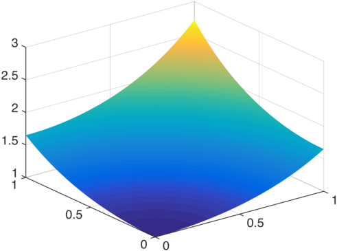
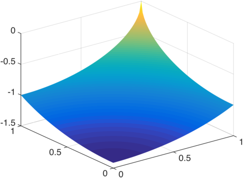
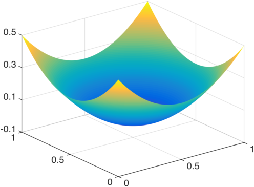
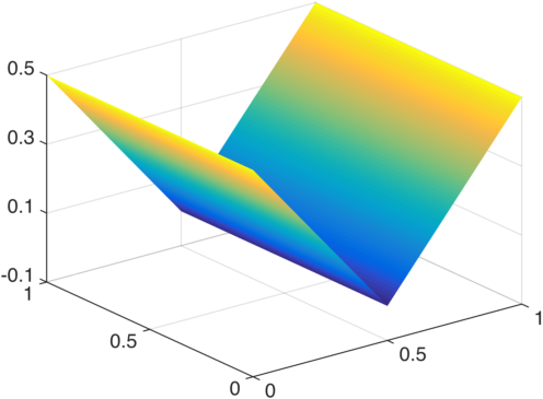
We provide numerical evidence for four scenarios. The data of the corresponding Monge-Ampère Dirichlet problems are given in Table 1. The results are reported in Tables 2, 3 and Figure 1.
| Test 1 | |||
|---|---|---|---|
| Test 2 | |||
| Test 3 | |||
| Test 4 |
| Test 1 | Test 2 | Test 3 | Test 4 | |
|---|---|---|---|---|
| 3.9093 | 2.5104 | 2.9143 | 1.7233 | |
| 1.0340 | 2.6475 | 1.1102 | 3.8580 | |
| 2.6643 | 2.2113 | 5.5511 | 1.0963 | |
| 6.6964 | 1.6920 | 3.0531 | 1.5155 | |
| 1.6781 | 1.2440 | 1.6098 | 2.3870 |
| Test 1 | Test 2 | Test 3 | Test 4 | |
|---|---|---|---|---|
| 2.2524 | 2.7012 | 6.3363 | 7.3175 | |
| 4.1574 | 2.6801 | 1.6653 | 1.0270 | |
| 1.1233 | 2.2223 | 5.5511 | 3.1919 | |
| 3.1368 | 1.6967 | 4.7184 | 6.5781 | |
| 1.3201 | 1.2500 | 2.1649 | 1.0464 |
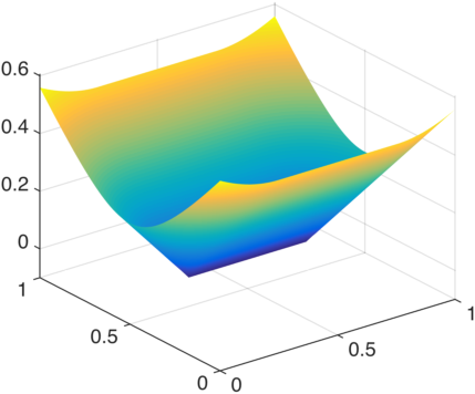
We conclude this section with numerical experiments for the Dirichlet problem for with using the standard finite difference discretization and the monotone scheme. The exact solution, taken from [6], is given by
Our results are reported on Tables 4, 5 and Figure 2. This example was chosen because many existing methods fail to capture the solution.
| 1.40 | 1.44 | 1.31 | 1.25 | 1.17 |
| 4.31 | 1.08 | 2.70 | 6.74 | 1.68 |

Remark 2.1.
Our numerical method also provides a technique for computing the convex envelope of boundary data and the convex envelope of a function defined on . We recall from [16] that given on (satisfying the assumptions of this paper), the convex envelope of on is the mimimum of over
Also given any function defined on , the convex envelope of is the minimum of over
References
- [1] N. E. Aguilera and P. Morin. Approximating optimization problems over convex functions. Numer. Math., 111(1):1–34, 2008.
- [2] G. Awanou. Iterative methods for -Hessian equations. http://arxiv.org/abs/1406.5366, 2013.
- [3] G. Awanou. Isogeometric method for the elliptic Monge-Ampère equation. In Approximation Theory, XIV (San Antonio, TX, 2013), pages 1–13. 2014.
- [4] G. Awanou. On standard finite difference discretizations of the elliptic Monge-Ampère equation. http://arxiv.org/abs/1311.2812, 2014.
- [5] G. Awanou and R. Awi. Convergence of stable and consistent schemes to the Aleksandrov solution of the Monge-Ampère equation. http://arxiv.org/abs/1507.08490, 2015.
- [6] J.-D. Benamou and B. D. Froese. A viscosity framework for computing Pogorelov solutions of the Monge-Ampère equation. http://arxiv.org/pdf/1407.1300v2.pdf, 2014.
- [7] S. C. Brenner, T. Gudi, M. Neilan, and L.-Y. Sung. penalty methods for the fully nonlinear Monge-Ampère equation. Math. Comp., 80(276):1979–1995, 2011.
- [8] A. Caboussat, R. Glowinski, and D. C. Sorensen. A least-squares method for the numerical solution of the Dirichlet problem for the elliptic Monge-Ampère equation in dimension two. ESAIM Control Optim. Calc. Var., 19(3):780–810, 2013.
- [9] S. K. Chung, A. K. Pani, and M. G. Park. Convergence of finite difference method for the generalized solutions of Sobolev equations. J. Korean Math. Soc., 34(3):515–531, 1997.
- [10] E. J. Dean and R. Glowinski. Numerical methods for fully nonlinear elliptic equations of the Monge-Ampère type. Comput. Methods Appl. Mech. Engrg., 195(13-16):1344–1386, 2006.
- [11] B. Froese and A. Oberman. Convergent finite difference solvers for viscosity solutions of the elliptic Monge-Ampère equation in dimensions two and higher. SIAM J. Numer. Anal., 49(4):1692–1714, 2011.
- [12] M. Grant. Disciplined Convex Programming. PhD thesis, Stanford University, 2004.
- [13] M. Grant and S. Boyd. CVX: Matlab software for disciplined convex programming, version 2.1. http://cvxr.com/cvx, Mar. 2014.
- [14] C. E. Gutiérrez. The Monge-Ampère equation. Progress in Nonlinear Differential Equations and their Applications, 44. Birkhäuser Boston Inc., Boston, MA, 2001.
- [15] D. Hartenstine. The Dirichlet problem for the Monge-Ampère equation in convex (but not strictly convex) domains. Electron. J. Differential Equations, pages No. 138, 9 pp. (electronic), 2006.
- [16] P.-L. Lions. Two remarks on Monge-Ampère equations. Ann. Mat. Pura Appl. (4), 142:263–275 (1986), 1985.
- [17] J. Rauch and B. A. Taylor. The Dirichlet problem for the multidimensional Monge-Ampère equation. Rocky Mountain J. Math., 7(2):345–364, 1977.
- [18] A. W. Roberts and D. E. Varberg. Convex functions. Academic Press [A subsidiary of Harcourt Brace Jovanovich, Publishers], New York-London, 1973. Pure and Applied Mathematics, Vol. 57.
- [19] N. Z. Shor. Nondifferentiable optimization and polynomial problems, volume 24 of Nonconvex Optimization and its Applications. Kluwer Academic Publishers, Dordrecht, 1998.
- [20] K. C. Toh, M. J. Todd, and R. H. Tütüncü. A MATLAB software package for semidefinite programming, version 1.3. 11(2):205–267, 1999.