Semidefinite relaxations in optimal experiment design with application to substrate injection for hyperpolarized MRI

Abstract

We consider the problem of optimal input design for estimating uncertain parameters in a discrete-time linear state space model, subject to simultaneous amplitude and $\ell_{1}$/$\ell_{2}$-norm constraints on the admissible inputs. We formulate this problem as the maximization of a (non-concave) quadratic function over the space of inputs, and use semidefinite relaxation techniques to efficiently find the global solution or to provide an upper bound. This investigation is motivated by a problem in medical imaging, specifically designing a substrate injection profile for in vivo metabolic parameter mapping using magnetic resonance imaging (MRI) with hyperpolarized carbon-13 pyruvate. In the $\ell_{2}$-norm-constrained case, we show that the relaxation is tight, allowing us to efficiently compute a globally optimal injection profile. In the $\ell_{1}$-norm-constrained case the relaxation is no longer tight, but can be used to prove that the boxcar injection currently used in practice achieves at least 98.7% of the global optimum.

I Introduction

I-A Optimal experiment design

In this paper we consider the problem of estimating uncertain parameters in a state space model from noisy output data. For such a system, the reliability of the parameter estimates depends on the choice of input used to excite the system, as some inputs provide greater information about the parameters than others. The problem of designing an input that is maximally informative is known as optimal experiment design and much work has been done on this problem in the last 50 years [1, 2, 3, 4].

Historically, most work on optimal experiment design for dynamic systems has focused on frequency domain techniques, where an optimal input is designed based on its power spectrum. Here, we approach this problem in the time domain, allowing us to impose amplitude ($\ell_{\infty}$) and $\ell_{1}$ constraints on the admissible inputs. Amplitude-constrained optimal experiment design is NP-hard in general [5], but semidefinite relaxation techniques can be used to generate approximate solutions and to bound the suboptimality of such solutions [5, 6]. In contrast with [5, 6], in this paper we restrict our attention to linear measures of the information allowing us to 1) write the objective function as a quadratic function of the input sequence and 2) apply an exactness result for quadratically constrained quadratic programming to give sufficient conditions under which the semidefinite relaxation recovers the global solution. We also present the results in terms of a state space model enabling us to model uncertainty in the initial state.

I-B Metabolic MRI using hyperpolarized substrates

We are motivated by a problem in metabolic magnetic resonance imaging (MRI) using hyperpolarized substrates. Hyperpolarized carbon-13 MRI has enabled the real-time observation of perfusion and metabolism in preclinical and clinical studies [7, 8, 9, 10, 11, 12]. This technology is made possible by techniques for dynamic nuclear polarization (DNP) that have led to signal-to-noise ratio (SNR) increases of four to five orders of magnitude compared with endogenous signal in dissolved ¹³C-labelled molecules [13, 14]. Injected [1-¹³C] pyruvate is frequently used as a substrate in metabolism experiments and its rate of conversion to [1-¹³C] lactate has been shown to distinguish between healthy and cancerous tissues in animal [8], and recently human [10], studies.

The goal of a metabolic MRI experiment is to learn the spatial distribution of metabolic rates, as this indicates the regions of the body where a particular metabolic pathway is active. Noise in the observed image data leads to uncertainty in estimates of metabolic rate parameters, but the amount of uncertainty can be mitigated with experiment design.

The problem of optimally designing an image acquisition sequence is considered in [15, 16]. In this paper we investigate optimal substrate injection profiles. After hyperpolarization the substrate must be injected into the test subject, where metabolism occurs and a sequence of images are acquired. Greater injection volumes lead to better signal-to-noise ratio, but for safety reasons the injection profile is limited by the rate at which substrate can be injected and by the total amount of fluid injected. Thus determining the optimal injection profile is of clinical interest.

I-C Outline

We begin in Section II by introducing the time domain optimal experiment design problem for linear systems, and discuss relevant relaxations from the literature. Then in Section III we present a mathematical model of hyperpolarized MRI and use semidefinite relaxation techniques to design optimal injection inputs for hyperpolarized substrates. We constrain the total amount of fluid injected using the $\ell_{2}$ or $\ell_{1}$ norms of the input signal. In the $\ell_{2}$-constrained case, the relaxation is tight and we are able to recover a globally optimal solution to the original problem. In the $\ell_{1}$-constrained case we do not recover a solution from the relaxation, but the objective value of the relaxation can be used to bound the optimality gap and show that a simple boxcar injection achieves at least 98.7% of the global optimum. Matlab code to reproduce the results in this paper is available at https://github.com/maidens/ACC-2016.

II Semidefinite relaxations in optimal experiment design

Consider a discrete-time linear system

$$\begin{split}x_{t+1}&=A(\theta)x_{t}+B(\theta)u_{t}\\ y_{t}&=Cx_{t}\\ Y_{t}&\sim N(y_{t},\Sigma)\end{split}$$ (1)

over a horizon $0\leq t\leq N$ where the initial state $x_{0}$ and time-invariant state dynamics matrices $A\in\mathbb{R}^{n\times n}$ and $B\in\mathbb{R}^{n\times n_{u}}$ are dependent on some unknown parameter vector $\theta\in\mathbb{R}^{p}$. We wish to choose an input sequence $u$ to maximize some measure of the Fisher information matrix

$$\mathcal{I}(\theta)=\sum_{t=0}^{N}(\nabla_{\theta}x_{t})^{T}C^{T}\Sigma^{-1}C(\nabla_{\theta}x_{t})$$ (2)

about the parameter vector $\theta$ contained in the data $Y$. The Fisher information is a positive semidefinite matrix that is used in experiment design for parameter estimation as a measure of the informativeness of an experiment [17, 4]. The inverse of the information gives an upper bound on the covariance of an arbitrary unbiased estimator $\theta$ via the Cramer-Rao inequality. See [18] for a derivation of (2).

II-A Quadratic objective function

We consider nonnegative, linear information metrics of the form

$$\varphi\big{(}\mathcal{I}(\theta)\big{)}=\operatorname{trace}\big{(}K\mathcal{I}(\theta)\big{)}$$ (3)

where $K\succeq 0$ is positive semidefinite. Particular cases include the T-optimal design criterion (where $K$ is the $p\times p$ identity matrix) [17] and the $c$-optimal design criterion (where $K=cc^{T}$) which is optimal for the scalar parameter $c^{T}\theta$ [19].

To formulate the problem of choosing the sequence $u_{k}$ for $k=0,\dots,N-1$ we define the stacked vector $\mathbf{u}=[u_{0}^{T}\dots u_{N-1}^{T}]^{T}$ and denote its components $\mathbf{u}^{(j,k)}$ where $(j,k)=kn_{u}+j$ defines a reverse lexicographic ordering, $j$ ranges over the input index from 1 to $n_{u}$ and $k$ ranges over the time index from 0 to $N-1$. With this notation established, we can state the following result.

Proposition 1

The objective (3) is a quadratic function

$$\varphi\big{(}\mathcal{I}(\theta)\big{)}=\mathbf{u}^{T}Q(\theta)\mathbf{u}+2q(\theta)^{T}\mathbf{u}+q_{0}(\theta)$$

of the design variable $\mathbf{u}$. The entries of the matrices appearing in the objective function are computed as

where $S_{hh^{\prime}}$ is the $hh^{\prime}$-th entry of $C^{T}\Sigma^{-1}C$, $m_{i}^{h}(t)$ is the $h$-th entry of the vector

$$A^{t}\frac{\partial x_{0}}{\partial\theta_{i}}+\sum_{\ell=0}^{t-1}A^{t-\ell-1}\frac{\partial A}{\partial\theta_{i}}A^{\ell}x_{0}$$

and $M_{kij}^{h}(t)$ is the $h,j$-th entry of the matrix

$$A^{t-k-1}\frac{\partial B}{\partial\theta_{i}}+\sum_{\ell=k+1}^{t-1}A^{t-\ell-1}\frac{\partial A}{\partial\theta_{i}}A^{\ell-k-1}B.$$

We see that for a linear dynamical system with Gaussian-distributed measurements, optimal experiment design is a nonconvex quadratic programming problem. If there are no constraints on the admissible inputs the optimal value is infinite, as by choosing $\mathbf{u}^{*}$ as an eigenvector of $Q(\theta)$ that corresponds to a nonzero eigenvalue, letting $\mathbf{u}=\alpha\mathbf{u}^{*}$ for $\alpha>0$, we can make $\mathbf{u}^{T}Q(\theta)\mathbf{u}+2q(\theta)^{T}\mathbf{u}+q_{0}(\theta)$ arbitrarily large.

Constrained quadratic programming is NP-hard in general [20]. But certain quadratic programming problems lend themselves to polynomial-time approximation algorithms using a semidefinite programming relaxation [21, 22]. We first give a proof of Proposition 1, before moving on to semidefinite relaxations of the optimal experiment design problem.

Proof:

Unrolling the recursion relation (1), we can write

$$x_{t}=A^{t}x_{0}+\sum_{k=0}^{t-1}A^{t-k-1}Bu_{k}.$$

Applying the chain rule to (1) we get a recursion relation for the sensitivities

$$\frac{\partial}{\partial\theta_{i}}x_{t+1}=A\frac{\partial}{\partial\theta_{i}}x_{t}+\frac{\partial A}{\partial\theta_{i}}x_{t}+\frac{\partial B}{\partial\theta_{i}}u_{t}$$

which can be unrolled as

To simplify notation, from this point forward we will use the Einstein summation convention, where upper and lower repeated indices denotes an implicit summation over those indices. In this notation, we see that the sensitivity matrix $\nabla_{\theta}x_{t}$ has entries

$$(\nabla_{\theta}x_{t})^{h}_{i}=M_{kij}^{h}(t)\mathbf{u}^{jk}+m_{i}^{h}(t)$$

where $M$ and $m$ are defined as in the statement of the proposition and the index $k$ runs from 0 to $t-1$. Thus the objective function is expressed as

∎

II-B Semidefinite relaxation of quadratic programs

Semidefinite relaxations of indefinite quadratic programming problems have been the subject of considerable study over the past two decades [21, 22, 23, 24, 25, 26]. The essential idea is to take a quadratic program

$$\begin{split}\textbf{maximize}&\ \ u^{T}Qu+2q^{T}u+q_{0}\\ \textbf{subject to}&\ \ u\in\mathcal{P}\subseteq\mathbb{R}^{d}\\ \end{split}$$ (4)

over a linear vector space and transform it to a linear problem over a quadratic space

$$\begin{split}\textbf{maximize}&\ \ \operatorname{trace}\left(\left[\begin{array}[]{cc}Q&q\\ q^{T}&q_{0}\end{array}\right]\left[\begin{array}[]{cc}U&u\\ u^{T}&1\end{array}\right]\right)\\ \textbf{subject to}&\ \ \left[\begin{array}[]{cc}U&u\\ u^{T}&1\end{array}\right]\in\tilde{\mathcal{P}}\subseteq\mathbb{R}^{(d+1)\times(d+1)}\\ &\ \ U=uu^{T}\end{split}$$ (5)

by introducing a rank 1 semidefinite variable $U=uu^{T}$ and translating the constraint set $\mathcal{P}$ from the the linear vector space to a convex constraint set $\tilde{\mathcal{P}}$ in the semidefinite matrix space. The problem (5) in non convex, but the equality constraint $U=uu^{T}$ can be relaxed to the inequality $U\succeq uu^{T}$ then transformed to semidefinite constraint $\left[\begin{array}[]{cc}U&u\\ u^{T}&1\end{array}\right]\succeq 0$ via Schur complement. Thus (5) can be relaxed to the convex problem

$$\begin{split}\textbf{maximize}&\ \ \operatorname{trace}\left(\left[\begin{array}[]{cc}Q&q\\ q^{T}&q_{0}\end{array}\right]\left[\begin{array}[]{cc}U&u\\ u^{T}&1\end{array}\right]\right)\\ \textbf{subject to}&\ \ \left[\begin{array}[]{cc}U&u\\ u^{T}&1\end{array}\right]\in\tilde{\mathcal{P}}\\ &\ \ \left[\begin{array}[]{cc}U&u\\ u^{T}&1\end{array}\right]\succeq 0.\end{split}$$ (6)

The value of the convex program (6) can then be used as an upper bound on the solution to (4). Further if a solution $\left[\begin{array}[]{cc}U^{*}&u^{*}\\ u^{*T}&1\end{array}\right]$ to (6) happens to have rank 1 then $u^{*}$ is a global solution to (4).

To translate constraints $u\in\mathcal{P}\subseteq\mathbb{R}^{d}$ on $u$ to constraints $U\in\tilde{\mathcal{P}}\subseteq\mathbb{R}^{d\times d}$ on $U$ there are a number of methods.

• Quadratic constraints on $u$ of the form

  $$\mathcal{P}=\{u:u^{T}Ru+2r^{T}u+r_{0}\leq 0\}$$

  are translated to constraints of the form

  $$\tilde{\mathcal{P}}=\{U:\operatorname{trace}\left(\left[\begin{array}[]{cc}R&r\\ r^{T}&r_{0}\end{array}\right]\left[\begin{array}[]{cc}U&u\\ u^{T}&1\end{array}\right]\right)\leq 0\}.$$

  For example, the $\ell_{2}$ constraint $\|u\|_{2}\leq c$ becomes $\operatorname{trace}(U)\leq c^{2}$.

• Amplitude constraints on $u$ of the form $\mathcal{P}=\{u:|u_{t}|\leq c_{t}\ t=1,\dots,d\}$ for particular constants $c_{t}$ are modelled as $d$ homogeneous quadratic constraints $\mathcal{P}=\{u:u_{t}^{2}\leq c_{t}^{2}\ t=1,\dots,d\}$ which correspond to $\tilde{\mathcal{P}}=\{U:U_{tt}\leq c_{t}^{2}\ t=1,\dots,d\}$.

• Box constraints of the form $\mathcal{P}=\{u:0\leq u_{t}\leq c_{t}\}$ can be translated as $\tilde{\mathcal{P}}=\{U:U_{tt}\leq c_{t}^{2}\ t=1,\dots,d\ \ \wedge\ \ U_{st}\geq 0\ s,t=1,\dots,d\}$.

• For $u$ normalized such that $0\leq u_{t}\leq 1$, the relaxation can be tightened by noting that $u_{i}^{2}\leq u_{i}$. Thus the constraints $U_{ii}\leq u_{i}\ \ i=1,\dots,d$ can be added to tighten the relaxation.

• If $u_{t}\geq 0$ and $a$ is a vector with $a_{t}\geq 0$ then the linear constraint $\mathcal{P}=\{u:a^{T}u\leq b\}$ can be translated by noting that $0\leq a^{T}u\leq b$ implies that $\operatorname{trace}(aa^{T}U)=\operatorname{trace}(a^{T}Ua)=a^{T}uu^{T}a=(a^{T}u)^{2}\leq b^{2}$. This results in a tighter approximation than adding the constraint $a^{T}u\leq b$ (see Lemma 1 of[27]). In particular, if we denote the $d\times d$ matrix of ones by $E$ then the $\ell_{1}$-norm constraint $\|u\|_{1}\leq b$ can be translated as $\operatorname{trace}(EU)\leq b^{2}$.

II-C A result on exact recovery from semidefinite relaxation

For a vector $u\in\mathbb{R}^{d}$ let $u^{2}$ denote the vector obtained by squaring the entries of $u$ component-wise and consider a problem of the form

$$\begin{split}\textbf{maximize}&\ \ u^{T}Qu+2q^{T}u+q_{0}\\ \textbf{subject to}&\ \ u^{2}\in\mathcal{F}.\\ \end{split}$$ (7)

The following result gives sufficient conditions for the semidefinite relaxation

$$\begin{split}\textbf{maximize}&\ \ \operatorname{trace}\left(\left[\begin{array}[]{cc}Q&q\\ q^{T}&q_{0}\end{array}\right]\left[\begin{array}[]{cc}U&u\\ u^{T}&1\end{array}\right]\right)\\ \textbf{subject to}&\ \ \operatorname{diag}(U)\in\mathcal{F}\\ &\ \ \left[\begin{array}[]{cc}U&u\\ u^{T}&1\end{array}\right]\succeq 0\end{split}$$ (8)

to recover the global solution of (7).

Proposition 2 (Adapted from Theorem 2 of [26])

If $Q_{ij}\geq 0$ for all $i\neq j$, $q_{i}\geq 0$ for all $i$ and $\mathcal{F}\subseteq\mathbb{R}^{d}$ is a closed convex set then the values of (7) and (8) coincide. Moreover, if $\tilde{U}^{*}$ is a solution of (8) then $\sqrt{\operatorname{diag}(\tilde{U}^{*})}$ is a solution of (7).

Thus if $u\in\mathcal{P}$ can be expressed in the form $u^{2}\in\mathcal{F}$ for some convex $\mathcal{F}$, and the entries of $Q$ and $q$ are nonnegative, we can globally solve (4) via the convex relaxation.

III Infusion input design for substrate injection in hyperpolarized carbon-13 MRI

We consider a linear model of magnetization exchange resulting from the injection of a hyperpolarized substrate, observed using a flip angle sequence $\alpha_{k,t}$ [28]:

where $AIF(t)$ is an arterial input function. The result of a bolus (impulse) injection of substrate is often modelled as the arterial input function is of the form [29]

$$AIF(t)=A_{0}t^{\gamma}e^{-t/\beta}.$$

In the case $\gamma=2$ the samples of this AIF can be modelled as the impulse response of the $\gamma+1=3$rd order system

We discretize (9) with step $\Delta t=2$ s assuming a zero-order hold on the AIF, yielding a model

$$\begin{split}\bar{x}_{t+1}&=\bar{A}\ \bar{x}_{t}+\bar{B}\ AIF_{t}\\ y_{t}&=\left[\begin{array}[]{ccccc}0&0&0&\sin(\alpha_{1,t})&0\\ 0&0&0&0&\sin(\alpha_{2,t})\end{array}\right]\bar{x}_{t}.\end{split}$$ (11)

Combining (10) and (11), we get a model of the full system (12) mapping the infusion input $u$ to the observed signals.

$$\begin{split}x_{t+1}&=\left[\begin{array}[]{ccccc}3e^{-(\Delta t)/\beta}&-3e^{-2(\Delta t)/\beta}&e^{-3(\Delta t)/\beta}&0&0\\ 1&0&0&0&0\\ 0&1&0&0&0\\ A_{0}e^{-(\Delta t)/\beta}\bar{B}_{1}&A_{0}e^{-2(\Delta t)/\beta}\bar{B}_{1}&0&\bar{A}_{11}&\bar{A}_{12}\\ A_{0}e^{-(\Delta t)/\beta}\bar{B}_{2}&A_{0}e^{-2(\Delta t)/\beta}\bar{B}_{2}&0&\bar{A}_{21}&\bar{A}_{22}\end{array}\right]x_{t}+\left[\begin{array}[]{c}1\\ 0\\ 0\\ 0\\ 0\end{array}\right]u_{t}\\ y_{t}&=\left[\begin{array}[]{ccccc}0&0&0&\sin(\alpha_{1,t})&0\\ 0&0&0&0&\sin(\alpha_{2,t})\end{array}\right]x_{t}\end{split}$$ (12)

We now solve an example instance of this system with model parameters taken from [16] which are shown in Table I , along with noise covariance matrix $\Sigma=I$, horizon of $N=30$ samples and a constant flip angle sequence $\alpha_{k,t}=15^{\circ}$. Computation times for solving this problem are given in Table II.

$R_{1P}$	$R_{1L}$	$k_{PL}$	$k_{TRANS}$	$t_{0}$	$\gamma$	$\beta$	$A_{0}$
1/10	1/10	0.07	0.055	3.2596	2.1430	3.4658	1.0411 $\times 10^{4}$

TABLE I: Nominal parameter values used

problem	time to generate SDP	SDP decision variable size	number of SDP constraints	time to solve SDP
$\ell_{2}$ constrained	12.0 s	30 $\times$ 30 symmetric	31	0.58 s
$\ell_{1}$ constrained		31 $\times$ 31 symmetric	497	5.51 s

TABLE II: Computation time to solve semidefinite programming relaxations. The SDP was solved using CVX [30] with the SeDuMi backend in MATLAB v8.4.0 running on a Macbook laptop (2.3 GHz quad-core Intel Core i7 Ivy Bridge processor, 8GB memory).

III-A $\ell_{2}$ constrained input

The substrate injection is constrained to limit the rate of injection to $|u_{t}|\leq 1$ and to limit the $\ell_{2}$ norm of the injection to $\|u\|_{2}\leq 4$. Thus we wish to solve the quadratically-constrained quadratic program

$$\begin{split}\textbf{maximize}&\ \ u^{T}Q(\theta)u\\ \textbf{subject to}&\ \ u_{t}^{2}\leq 1\\ &\ \ \sum_{t=0}^{N-1}u_{t}^{2}\leq 16.\end{split}$$ (13)

The matrix $Q$ is nonnegative and the constraints are of the form $u^{2}\in\mathcal{F}$ where $\mathcal{F}$ is a closed convex set. Therefore this problem yields a semidefinite relaxation

$$\begin{split}\textbf{maximize}&\ \ \operatorname{trace}\Big{(}Q(\theta)U\Big{)}\\ \textbf{subject to}&\ \ U_{tt}\leq 1\\ &\ \ \operatorname{trace}(U)\leq 16.\end{split}$$ (14)

whose solution has rank 1 (by Proposition 2). So we can extract a globally optimal solution to (13) from its semidefinite relaxation. The resulting optimal input trajectory and the corresponding output trajectories are shown in Fig. 1.

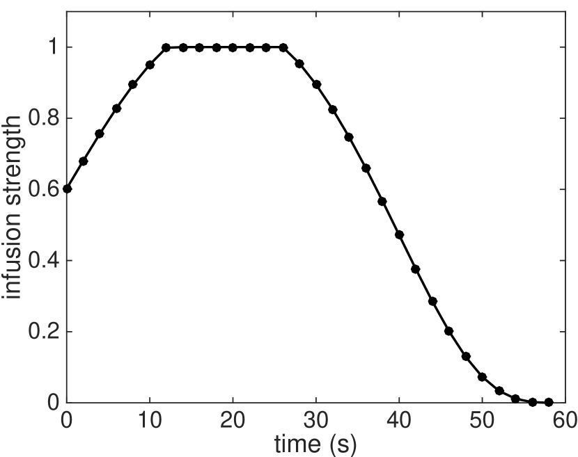
(a) Optimal input

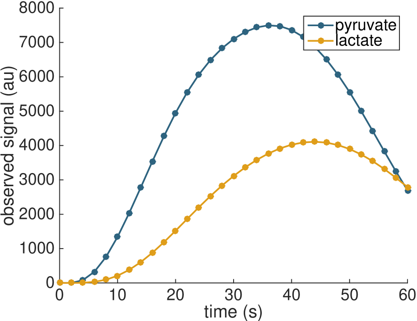
(b) Corresponding outputs

Figure 1: Optimal solution to (13) computed using semidefinite relaxation.

III-B $\ell_{1}$ constrained input

We now replace the $\ell_{2}$-norm constraint with an $\ell_{1}$-norm constraint $\|u\|_{1}\leq 8$ that limits the total amount of substrate injected. This constraint is more clinically relevant than the $\ell_{2}$-norm constraint, as the total substrate than can be injected is often limited due to safety-related concerns. This leads to a linearly-constrained QP of the form

$$\begin{split}\textbf{maximize}&\ \ u^{T}Q(\theta)u\\ \textbf{subject to}&\ \ 0\leq u_{t}\leq 1\\ &\ \ \sum_{t=0}^{N-1}u_{t}\leq 8.\end{split}$$ (15)

This QP can be relaxed to the semidefinite program

$$\begin{split}\textbf{maximize}&\ \ \operatorname{trace}\Big{(}Q(\theta)U\Big{)}\\ \textbf{subject to}&\ \ \left[\begin{array}[]{cc}U&u\\ u^{T}&1\end{array}\right]\succeq 0\\ &\ \ U_{tt}\leq u_{t}\\ &\ \ \operatorname{trace}\Big{(}EU\Big{)}\leq 64\\ &\ \ U_{st}\geq 0\end{split}$$ (16)

where both $U$ and $u$ are decision variables and $E$ is the $N\times N$ matrix of ones. In this case, the constraint set is more complex than in the $\ell_{2}$-norm constrained case. Therefore the solution to the semidefinite program does not have rank 1, so we cannot extract the solution to (15). But the optimal value of (16) is an upper bound on the optimal value of (15), so given a proposed solution of (15) we can bound the optimality gap using the value of (16).

We conjecture that the global solution of (15) is the boxcar shown in Fig. 2. This input is what is currently used in practice: the substrate is injected at the maximum rate until the total allowable volume has been injected. Comparing the optimal value $1.2888\times 10^{10}$ of the relaxation with the objective value $1.2724\times 10^{10}$ we see that the boxcar input achieves a value of a factor of at least 0.9873 the optimal value. Thus even if our conjecture is incorrect and the boxcar is not optimal, the improvement that may be achieved by the optimal input is negligible. This observation helps to validate the current practice in hyperpolarized MRI.

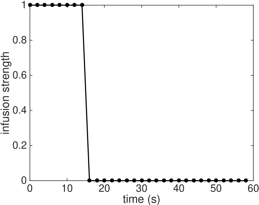
(a) Boxcar input

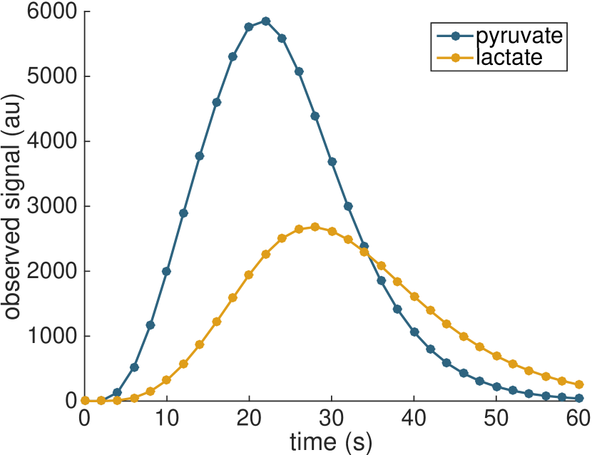
(b) Corresponding outputs

Figure 2: The boxcar input function, which we conjecture to be optimal for the $\ell_{1}$-constrained problem.

IV Conclusions

We have found that semidefinite relaxation can be used to compute an optimal hyperpolarized substrate infusion input profile for estimating uncertain metabolic rate parameters in metabolic MRI. Future work will focus on investigating the relationship between the rank 1 recovery that we see in the $\ell_{2}$-norm-constrained case and properties of the dynamic system such as positivity and passivity, and attempting to extend these results to nonlinear measures of the information such as the D- E- and A-optimality criteria used in [6].

References

- [1] M. Gevers, X. Bombois, R. Hildebrand, and G. Solari, “Optimal experiment design for open and closed-loop system identification,” Communications in Information and Systems, vol. 11, no. 3, pp. 197–224, 2011.
- [2] G. Goodwin and R. Payne, Dynamic System Identification: Experiment Design and Data Analysis. Academic Press, 1977.
- [3] L. Ljung, System Identification: Theory for the User. Pearson Education, 1999.
- [4] É. Walter and L. Pronzato, Identification of parametric models from experimental data, ser. Communications and control engineering. Springer, 1997.
- [5] I. R. Manchester, “Amplitude-constrained input design: Convex relaxation and application to clinical neurology,” in SYSID2012: IFAC Symposium on System Identification, 2012.
- [6] ——, “Input design for system identification via convex relaxation,” in 49th IEEE Conference on Decision and Control (CDC), 2010, pp. 2041–2046.
- [7] K. Golman and S. J. Petersson, “Metabolic imaging and other applications of hyperpolarized 13C1,” Academic Radiology, vol. 13, no. 8, pp. 932–942, 2006.
- [8] S. E. Day, M. I. Kettunen, F. A. Gallagher, D.-E. Hu, M. Lerche, J. Wolber, K. Golman, J. H. Ardenkjaer-Larsen, and K. M. Brindle, “Detecting tumor response to treatment using hyperpolarized 13C magnetic resonance imaging and spectroscopy,” Nature Medicine, no. 11, pp. 1382–1387, 2007.
- [9] S. M. Kazan, S. Reynolds, A. Kennerley, E. Wholey, J. E. Bluff, J. Berwick, V. J. Cunningham, M. N. Paley, and G. M. Tozer, “Kinetic modeling of hyperpolarized 13C pyruvate metabolism in tumors using a measured arterial input function,” Magnetic Resonance in Medicine, vol. 70, no. 4, pp. 943–953, 2013.
- [10] S. J. Nelson, J. Kurhanewicz, D. B. Vigneron, P. E. Z. Larson, A. L. Harzstark, M. Ferrone, M. van Criekinge, J. W. Chang, R. Bok, I. Park, G. Reed, L. Carvajal, E. J. Small, P. Munster, V. K. Weinberg, J. H. Ardenkjaer-Larsen, A. P. Chen, R. E. Hurd, L.-I. Odegardstuen, F. J. Robb, J. Tropp, and J. A. Murray, “Metabolic imaging of patients with prostate cancer using hyperpolarized [1-13C]pyruvate,” Science Translational Medicine, vol. 5, no. 198, p. 198ra108, 2013.
- [11] N. Bahrami, C. L. Swisher, C. von Morze, D. B. Vigneron, and P. E. Z. Larson, “Kinetic and perfusion modeling of hyperpolarized 13C pyruvate and urea in cancer with arbitrary RF flip angles,” Quantitative Imaging in Medicine and Surgery, vol. 4, no. 1, 2014.
- [12] C. L. Swisher, P. E. Z. Larson, K. Kruttwig, A. B. Kerr, S. Hu, R. A. Bok, A. Goga, J. M. Pauly, S. J. Nelson, J. Kurhanewicz, and D. B. Vigneron, “Quantitative measurement of cancer metabolism using stimulated echo hyperpolarized carbon-13 MRS,” Magnetic Resonance in Medicine, vol. 71, no. 1, pp. 1–11, 2014.
- [13] J. H. Ardenkjær-Larsen, B. Fridlund, A. Gram, G. Hansson, L. Hansson, M. H. Lerche, R. Servin, M. Thaning, and K. Golman, “Increase in signal-to-noise ratio of 10,000 times in liquid-state NMR,” Proceedings of the National Academy of Sciences, vol. 100, no. 18, pp. 10 158–10 163, 2003.
- [14] K. Golman, J. H. Ardenkjær-Larsen, J. S. Petersson, S. Mansson, and I. Leunbach, “Molecular imaging with endogenous substances,” Proceedings of the National Academy of Sciences, vol. 100, no. 18, pp. 10 435–10 439, 2003.
- [15] J. Maidens, P. E. Z. Larson, and M. Arcak, “Optimal experiment design for physiological parameter estimation using hyperpolarized carbon-13 magnetic resonance imaging,” in Proceedings of the American Control Conference, 2015.
- [16] J. Maidens, J. W. Gordon, P. E. Z. Larson, and M. Arcak, “Optimizing flip angles for metabolic rate estimation in hyperpolarized carbon-13 MRI,” IEEE Transactions on Medical Imaging, Submitted. [Online]. Available: http://www.eecs.berkeley.edu/~maidens/papers/2016TMI.pdf
- [17] F. Pukelsheim, Optimal design of experiments, ser. Probability and mathematical statistics. Wiley, 1993.
- [18] J. Maidens and M. Arcak, “A note on optimal experiment design for nonlinear systems using dynamic programming,” ArXiv e-prints, 2015. [Online]. Available: http://arxiv.org/abs/1503.07232
- [19] F. Pukelsheim, “On c-optimal design measures,” Series Statistics, vol. 12, no. 1, pp. 13–20, 1981.
- [20] M. Garey and D. Johnson, Computers and Intractability: A Guide to the Theory of NP-Completeness, ser. A Series of books in the mathematical sciences. W. H. Freeman, 1979.
- [21] M. X. Goemans and D. P. Williamson, “Improved approximation algorithms for maximum cut and satisfiability problems using semidefinite programming,” J. Assoc. Comput. Mach., vol. 42, pp. 1115–1145, 1995.
- [22] Z.-Q. Luo, W.-K. Ma, A.-C. So, Y. Ye, and S. Zhang, “Semidefinite relaxation of quadratic optimization problems,” IEEE Signal Processing Magazine, vol. 27, no. 3, pp. 20–34, 2010.
- [23] Y. Nesterov, “Semidefinite relaxation and nonconvex quadratic optimization,” Optimization Methods and Software, vol. 9, no. 1-3, pp. 141–160, 1998.
- [24] A. Nemirovski, C. Roos, and T. Terlaky, “On maximization of quadratic form over intersection of ellipsoids with common center,” Mathematical Programming, vol. 86, no. 3, pp. 463–473, 1999.
- [25] Y. Ye, “Approximating quadratic programming with bound and quadratic constraints,” Mathematical Programming, vol. 84, no. 2, pp. 219–226, 1999.
- [26] S. Zhang, “Quadratic maximization and semidefinite relaxation,” Mathematical Programming, vol. 87, no. 3, pp. 453–465, 2000.
- [27] C. Helmberg, F. Rendl, and R. Weismantel, “Quadratic knapsack relaxations using cutting planes and semidefinite programming,” in Integer Programming and Combinatorial Optimization, ser. Lecture Notes in Computer Science, W. H. Cunningham, S. McCormick, and M. Queyranne, Eds. Springer Berlin Heidelberg, 1996, vol. 1084, pp. 175–189.
- [28] O. Khegai, R. F. Schulte, M. A. Janich, M. I. Menzel, E. Farrell, A. M. Otto, J. H. Ardenkjaer-Larsen, S. J. Glaser, A. Haase, M. Schwaiger, and F. Wiesinger, “Apparent rate constant mapping using hyperpolarized [1-13C]pyruvate,” NMR in Biomedicine, vol. 27, no. 10, pp. 1256–1265, 2014.
- [29] C. von Morze, P. E. Z. Larson, S. Hu, K. Keshari, D. M. Wilson, J. H. Ardenkjaer-Larsen, A. Goga, R. Bok, J. Kurhanewicz, and D. B. Vigneron, “Imaging of blood flow using hyperpolarized [13C]urea in preclinical cancer models,” Journal of Magnetic Resonance Imaging, vol. 33, no. 3, pp. 692–697, 2011.
- [30] M. Grant and S. Boyd, “CVX: Matlab software for disciplined convex programming, version 2.1,” http://cvxr.com/cvx, Mar. 2014.