Mesh Grading in Isogeometric Analysis

Abstract

This paper is concerned with the construction of graded meshes for approximating so-called singular solutions of elliptic boundary value problems by means of multipatch discontinuous Galerkin Isogeometric Analysis schemes. Such solutions appear, for instance, in domains with re-entrant corners on the boundary of the computational domain, in problems with changing boundary conditions, in interface problems, or in problems with singular source terms. Making use of the analytic behavior of the solution, we construct the graded meshes in the neighborhoods of such singular points following a multipatch approach. We prove that appropriately graded meshes lead to the same convergence rates as in the case of smooth solutions with approximately the same number of degrees of freedom. Representative numerical examples are studied in order to confirm the theoretical convergence rates and to demonstrate the efficiency of the mesh grading technology in Isogeometric Analysis.

1 Introduction

The gradient of the solution of elliptic boundary value problems can exhibit singularities in the vicinities of re-entrant corners or edges. The same is true in case of changing boundary conditions or interface problems. This singular behavior of the gradients was discovered and analyzed in the famous work by Kondrat’ev [19]. We refer the reader to the monographs [14, 15, 20] for a more recent and comprehensive presentation of related results. It is well known that these singularities may cause loss in the approximation order of the standard discretization methods like the finite element method, see the classical monograph [29] or the more recent paper [6]. In the case of two dimensional problems with singular boundary points, grading mesh techniques have been developed for finite element methods in order to recover the full approximation order, see the classical textbook [25] and the more recent publications [6, 5, 13], and [3] for three-dimensional problems. Here, we devise graded meshes for solving elliptic problems with singular solutions by means of discontinuous Galerkin Isogeometric Analysis method (dG IgA).

In the IgA frame, the use of B-splines or NURBS basis functions allow complicated CAD geometries to be exactly represented, and the key point of Hughes et al. [16] was to make use of the same basis to approximate the solution of the problem under consideration. Since this pioneer paper, applications of IgA method have been considered in many fields, see [9]. Here, we apply a multipatch symmetric dG IgA method which has been extensively studied for diffusion problems in volumetric computational domains and on surfaces in [24] and [23], respectively, see also [22] for comprehensive presentation. The solution of the problem is independently approximated in every subdomain by IgA, without imposing any matching grid conditions and without any continuity requirements for the discrete solution across the subdomain interfaces. Symmetrized numerical fluxes with interior penalty jump terms, see, e.g., [11, 27, 10], are introduced on the interfaces in order to treat the discontinuities of the discrete solution and to interchange information between the non matching grids. As we will see later, the consideration of the numerical scheme in this general context makes it more flexible to be applied on zone-type subdivisions of $\Omega$, which have been found to be quite convenient for treating elliptic boundary value problems in domains with singular boundary points.

This paper aims at the construction of graded dG IgA meshes in the zones located near the singular points in order to recover full convergence rates like in the case of smooth solutions on uniform meshes. The grading of the mesh is mainly determined by the analytic behavior of the solution $u$ around the singular points and follows the spirit of grading mesh techniques using layers, which have been proposed for finite element methods in [25, 6, 5]. According to this, having an a priori knowledge about the location of the singular point, e.g. the re-entrant corner, the domain $\Omega$ is subdivided into zones, called layers in [6, 5], and then a further subdivision of $\Omega$ into subdomains (also called patches in IgA), say $\mathcal{T}_{H}(\Omega):=\{\Omega_{i}\}_{i=1}^{N}$, is performed in such way that $\mathcal{T}_{H}(\Omega)$ is in correspondence with the initial zone partition. On the other hand, the solution can be split into a sum of a regular part $u_{r}\in W^{l\geq 2,2}(\Omega)$ and a singular part $u_{s}\in W^{1+\varepsilon,2}(\Omega)$, with known $\varepsilon\in(0,1)$, i.e., $u=u_{r}+u_{s}$, see, e.g., [14]. The analytical form of $u_{s}$ contains terms with singular exponents in the radial direction. We use this information and construct appropriately graded meshes in the zones around the singular points. The resulting graded meshes have a “zone-wise character”, this means that the grid size of the graded mesh in every zone determines the mesh of every subdomain which belongs into this zone, where we assume that every subdomain belongs to only one zone (the ideal situation is every zone to be a subdomain). We mention that the mesh grading methodology is developed and is analyzed for the classical two dimensional problem with a re-entrant corner. The proposed methodology can be generalized and applied to other situations. This is shown by the numerical examples presented in Section 4.

The particular properties of the produced graded meshes help us to show optimal error estimates for the dG IgA method, which exhibit optimal convergence rates. The error estimates for the proposed method are proved by using a variation of Céa’s Lemma and using B-spline quasi-interpolation estimates for $u\in W^{1,2}(\Omega)\cap W^{l\geq 2,p\in(1,2]}(\mathcal{T}_{H}(\Omega))$, which have been proved in [24]. More precisely, these interpolation estimates have subdomain character and are expressed with respect to the mesh size $h_{i}$ of the corresponding subdomain $\Omega_{i}$. For the domains away from the singular point, the solution is smooth (see $u_{r}$ part in previous splitting), and we can derive the usual interpolation estimates. Conversely, for the subdomains $\Omega_{i}$, for which the boundary $\partial\Omega_{i}$ touches the singular point, the singular part $u_{s}$ of the solution $u$ can be considered as a function from the Sobolev space $W^{2,p\in(1,2)}(\Omega_{i})$. Now the estimates given in [24] enable us to derive error estimates for the singular part $u_{s}$. This makes the whole error analysis easier in comparison with the techniques earlier developed for the finite element method, e.g., in [6, 2, 13].

We mention that, in the literature, other IgA techniques have been proposed for solving two-dimensional problems with singularities very recently. In [26] and [17], the mapping technique has been developed, where the original B-spline finite dimensional space has been enriched by generating singular functions which resemble the types of the singularities of the problem. The mappings constructed on this enriched space describe the geometry singularities explicitly. Also in [8], by studying the anisotropic character of the singularities of the problem, the one-dimensional approximation properties of the B-splines are generalized for two-dimensional problems, in order to produce anisotropic refined meshes in the regions of the singular points.

The rest of the paper is organized as follows. The problem description, the weak formulation and the dG IgA discrete analogue are presented in Section 2. Section 3 discusses the construction of the appropriately graded IgA meshes, and provides the proof for obtaining the full approximation order of the dG IgA method on the graded meshes. Several two and three dimensional examples are presented in Section 4. Finally, we draw some conclusion.

2 Problem description and dG IgA discretization

First, let us introduce some notation. We define the differential operator

$$D^{a}=D_{1}^{\alpha_{1}}\cdot\cdot\cdot D_{d}^{\alpha_{d}},\text{with}{\ }D_{j}=\frac{\partial}{\partial x_{j}},D^{(0,...,0)}u=u,$$ (2.1)

where $\alpha=(\alpha_{1},...,\alpha_{d})$, with $\alpha_{j}\geq 0,j=1,...,d$, denotes a multi-index of the degree $|\alpha|=\sum_{j=1}^{d}\alpha_{j}$. For a bounded Lipschitz domain $\Omega\subset\mathbb{R}^{d}$, $d=2,3$ we denote by $W^{l,p}(\Omega)$, with $l\geq 1$ and $1\leq p\leq\infty$, the usual Sobolev function spaces endowed with the norms

$$\|u\|_{W^{l,p}(\Omega)}=\big{(}\sum_{0\leq|\alpha|\leq m}\|D^{\alpha}u\|_{L^{p}(\Omega)}^{p}\big{)}^{\frac{1}{p}},$$ (2.2a)

$$\|u\|_{W^{l,\infty}(\Omega)}=max_{0\leq|\alpha|\leq m}\|D^{\alpha}u\|_{\infty}.$$ (2.2b)

More details about Sobolev’s function spaces can be found in [1]. We often write $a\sim b$, meaning that $C_{m}a\leq b\leq C_{M}a$, with $C_{m}$ and $C_{M}$ are positive constants independent of the discretization parameters.

2.1 The model problem

Let us assume that the boundary of $\Gamma_{D}=\partial\Omega$ of $\Omega$ contains geometric singular parts. In particular, for $d=2$, we consider domains which have corner boundary points with internal angles greater than $\pi$. For $d=3$, we consider that case where the domain $\Omega$ can be described in the form $\Omega=\Omega_{2}\times Z$, where $\Omega_{2}\subset\mathbb{R}^{2}$ and $Z=[0,z_{M}]$ is an interval. The cross section of $\Omega$ has only one corner with an interior angle $\omega\in(\pi,2\pi)$. This means that the $\partial\Omega$ has only one singular edge which is $\Gamma_{s}:=\{(0,0,z),0\leq z\leq z_{M}\}$. The remaining parts of $\Gamma_{D}$ are considered as smooth, see Fig. 2(a) and Fig. 2(b) for an illustration of the domains.

For simplicity, we restrict our study to the following model problem

$$-\mathrm{div}(\alpha\nabla u)=f\quad\text{in}\quad\Omega,\quad u=u_{D}\quad\text{on}\quad\partial\Omega,$$ (2.3)

where the coefficient $\alpha(x)\in L^{\infty}(\Omega)$ is a piecewise constant function, bounded from above and below by positive constants, $f\in L^{2}(\Omega)$ and $u_{D}\in H^{\frac{1}{2}}(\partial\Omega)$ are given data. The variational formulation of (2.3) reads as follows: find $u\in W^{1,2}(\Omega)$ such that $u=u_{D}$ on $\Gamma_{D}=\partial\Omega$ and

$$a(u,v)=l(v),\quad\forall v\in W^{1,2}_{0}(\Omega),\qquad$$ (2.4a)

where

$$a(u,v)=\int_{\Omega}\alpha\nabla u\cdot\nabla v\,dx\quad\mbox{and}\quad l(v)=\int_{\Omega}fv\,dx.$$ (2.4b)

It is clear that, under the assumptions made above, there exists a unique solution of the variational problem (2.4) due to Lax-Milgram’s lemma.

We follow the theoretical analysis of the regularity of solution presented in [15]. We consider the two-dimensional case. Suppose that the $\Gamma_{D}$ has only one singular corner, say $P_{s}$, with internal angle $\omega\in(\pi,2\pi)$, and that the boundary parts from the one and the other side of $P_{s}$ are straight lines, see Fig. 2(a). We consider the local cylindrical coordinates $(r,\theta)$ with origin $P_{s}$, and define the cone (a circular sector with angular point $P_{s}$).

$${\mathcal{C}=\{(x,y)\in\Omega:x=r\cos(\theta),y=r\sin(\theta),0<r<R,0<\theta<\omega\}.}$$ (2.5)

We construct a highly smooth cut-off function $\xi$ in $\mathcal{C}$, such that $\xi\in C^{\infty}$, and it is supported inside the cone $\mathcal{C}$. It has been shown in [15], that the solution $u$ of the problem (2.4) can be written as a sum of a regular function $u_{r}\in W^{l\geq 2,2}(\Omega)$ and a singular function $u_{s}$,

$$u=u_{r}+u_{s},$$ (2.6)

with

$$u_{s}=\xi(r)\gamma r^{\lambda}\sin(\lambda\theta),$$ (2.7)

where $\gamma$ is the stress intensity factor (for the two-dimensional problems is a real number depending only on $f$) and $\lambda=\frac{\pi}{\omega}\in(0,1)$ is an exponent which determines the strength of the singularity. Since $\lambda<1$, by an easy computation, we can show that the singular function $u_{s}$ does not belong to $W^{2,2}(\Omega)$ but to $W^{l=2,p}(\Omega)$ with $p={2}/{(2-\lambda)}$. Consequently, the regularity properties of $u$ in $\mathcal{C}$ are mainly determined by the regularity properties of $u_{s}$, and we can assume that $u\in W^{1,2}(\Omega)\cap W^{l,p}(\mathcal{T}_{H}(\Omega))$, (see below details for the $\mathcal{T}_{H}(\Omega)$).

Remark 1

For the expression (2.7), we admit that the computational domain has only one non-convex corner and only Dirichlet boundary conditions are prescribed on $\partial\Omega$. Similar expression can be derived if there are more non-convex corners and if there are other type of boundary conditions, see details in [15].

2.2 The dG IgA discrete scheme

2.2.1 Isogeometric Analysis Spaces

We assume a non-overlapping subdivision $\mathcal{T}_{H}(\Omega):=\{\Omega_{i}\}_{i=1}^{N}$ of the computational domain $\Omega$ such that $\bar{\Omega}=\bigcup_{i=1}^{N}\bar{\Omega}_{i}$ with $\Omega_{i}\cap\Omega_{j}=\emptyset$ for $i\neq j$. The subdivision $\mathcal{T}_{H}(\Omega)$ is considered to be compatible with the discontinuities of the coefficient $\alpha$, i.e., the jumps can only appear on the interfaces $F_{ij}=\partial\Omega_{i}\cap\partial\Omega_{j}$ between the subdomains. For the sake of brevity in our notations, the set of common interior faces are denoted by $\mathcal{F}_{I}$. The collection of the faces that belong to $\partial\Omega$ are denoted by $\mathcal{F}_{B}$, i.e., $F\in\mathcal{F}_{B}$, if there is a $\Omega_{i}\in\mathcal{T}_{H}(\Omega)$ such that $F=\partial\Omega_{i}\cap\partial\Omega$. We denote the set of all subdomain faces by $\mathcal{F}=\mathcal{F}_{I}\cup\mathcal{F}_{B}.$

In the multi-patch (multi-subdomain) IgA context, each subdomain is represented by a B-spline (or NURBS) mapping. To accomplish this, we associate each $\Omega_{i}$ with a vector of knots $\mathbf{\Xi}^{d}_{i}=(\Xi_{i}^{1},...,\Xi_{i}^{\iota},...,\Xi_{i}^{d})$, with $\Xi_{i}^{\iota}=\{\mathbf{\xi}^{\iota}_{1},\mathbf{\xi}_{2}^{\iota},...,\xi_{n}^{\iota}\}$, $\iota=1,\ldots,d$, which are set on the parametric domain $\widehat{\Omega}=(0,1)^{d}$. The interior knots of $\mathbf{\Xi}^{d}_{i}$ are considered without repetitions and form a mesh $T^{(i)}_{h_{i},\widehat{\Omega}}=\{\hat{E}_{m}\}_{m=1}^{M_{i}}$ in $\widehat{\Omega}$, where $\hat{E}_{m}$ are the micro elements. Given a micro element $\hat{E}_{m}\in T^{(i)}_{h_{i},\widehat{\Omega}}$, we denote by $h_{\hat{E}_{m}}=diameter(\hat{E}_{m})$, and the local grid size $h_{i}$ is defined to be the maximum diameter of all $\hat{E}_{m}\in T^{(i)}_{h_{i},\widehat{\Omega}}$, that is $h_{i}=\max\{h_{\hat{E}_{m}}\}$. We refer the reader to [9] for more information about the meaning of the knot vectors in CAD and IgA.

Assumption 1

The meshes $T^{(i)}_{h_{i},\widehat{\Omega}}$ defined by the knots $\mathbf{\Xi}^{d}_{i}$ are quasi-uniform, i.e., there exist a constant $\sigma\geq 1$ such that $\sigma^{-1}\leq\frac{h_{\hat{E}_{m}}}{h_{\hat{E}_{m+1}}}\leq\sigma$.

On each $T^{(i)}_{h_{i},\widehat{\Omega}}$, we derive the finite dimensional space $\hat{\mathbb{B}}^{(i)}_{h_{i}}$ spanned by B-spline (or NURBS) basis functions of degree $k$, see more details in [9, 7, 28],

$$\hat{\mathbb{B}}^{(i)}_{h_{i}}=span\{\hat{B}_{\mathbf{j}}^{(i)}(\hat{x})\}_{\mathbf{j}=0}^{dim(\hat{\mathbb{B}}_{h_{i}}^{(i)})}.$$ (2.8a)

Every $$\hat{B}_{\mathbf{j}}^{(i)}(\hat{x})$$ function in (2.8a) is derived by means of tensor products of one-dimensional B-spline basis functions, i.e.

$$\hat{B}_{\mathbf{j}}^{(i)}(\hat{x})=\hat{B}_{\iota=1,j_{1}}^{(i)}(\hat{x}_{1})\cdot\cdot\cdot\hat{B}_{\iota=d,j_{d}}^{(i)}(\hat{x}_{d}).$$ (2.8b)

In the following, we suppose that the one-dimensional B-splines in (2.8b) have the same degree $k$. Finally, having the B-spline spaces, we can represent each subdomain $\Omega_{i}$ by the parametric mapping

$$\mathbf{\Phi}_{i}:\widehat{\Omega}\rightarrow\Omega_{i}, \quad\mathbf{\Phi}_{i}(\hat{x})=\sum_{\mathbf{j}}C^{(i)}_{\mathbf{j}}\hat{B}_{\mathbf{j}}^{(i)}(\hat{x}):=x\in\Omega_{i},$$ (2.9a)

with $$\quad\hat{x}=\mathbf{\Psi}_{i}(x):=\mathbf{\Phi}^{-1}_{i}(x),$$ (2.9b)

where $C_{\mathbf{j}}^{(i)}$ are the B-spline control points, $i=1,...,N$, cf. [9].

We construct a mesh $T^{(i)}_{h_{i},\Omega_{i}}=\{E_{m}\}_{m=1}^{M_{i}}$ for every $\Omega_{i}$, whose vertices are the images of the vertices of the corresponding parametric mesh $T^{(i)}_{h_{i},\widehat{\Omega}}$ through $\mathbf{\Phi}_{i}$. Notice that, the above subdomain mesh construction can result in non-matching meshes along the patch interfaces.

Further, by taking advantage of the properties of $\mathbf{\Phi}_{i}$, we define the global finite dimensional B-spline (dG) space

$$\mathbb{B}_{h}(\mathcal{T}_{H}):=\mathbb{{B}}^{(i)}_{h_{i}}(\Omega_{i})\times...\times\mathbb{{B}}^{(N)}_{h_{N}}(\Omega_{N}),$$ (2.10a)

where every $$\mathbb{B}^{(i)}_{h_{i}}(\Omega_{i}) T^{(i)}_{h_{i},\Omega_{i}}$$ is defined on as follows:

$$\mathbb{B}^{(i)}_{h_{i}}(\Omega_{i}):=\{B_{\mathbf{j}}^{(i)}|_{\Omega_{i}}:B_{\mathbf{j}}^{(i)}({x})=\hat{B}_{\mathbf{j}}^{(i)}\circ\mathbf{\Psi}_{i}({x}),{\ }\text{for}{\ }\hat{B}_{\mathbf{j}}^{(i)}\in\hat{\mathbb{B}}^{(i)}_{h_{i}}\}.$$ (2.10b)

Later, the solution $u$ of the problem (2.4) will be approximated by the discrete (dG) solution $u_{h}\in\mathbb{B}_{h}(\mathcal{T}_{H})$.

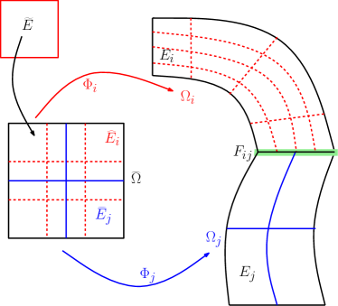
Figure 1: The parametric domain and two adjacent subdomains with different underlying meshes red and blue.

2.2.2 Discrete Problem

The problem (2.4) is independently discretized in every $\Omega_{i}$ using the spaces (2.10b) without imposing continuity requirements for the B-spline basis functions on the interfaces $F_{ij}=\partial\Omega_{i}\cap\partial\Omega_{j}$ and also non-matching grids may exist. Using the notation $\phi_{h}^{(i)}:=\phi_{h}|_{\Omega_{i}}$, we define the average and the jump of $\phi_{h}\in\mathbb{B}_{h}(\mathcal{T}_{H})$ on $F_{ij}\in\mathcal{F}_{I}$ by

$$\{\phi_{h}\}:=\frac{1}{2}(\phi_{h}^{(i)}+\phi_{h}^{(j)}), {\ }\text{and}\qquad\llbracket\phi_{h}\rrbracket:=\phi_{h}^{(i)}-\phi_{h}^{(j)},$$ (2.11a)

and, for $$F_{i}\in\mathcal{F}_{B}$$,

$$\{\phi_{h}\}:=\phi_{h}^{(i)}, {\ }\text{and}\qquad\llbracket\phi_{h}\rrbracket:=\phi_{h}^{(i)}.$$ (2.11b)

The discrete problem is specified by the symmetric dG IgA method, see [24], and reads as follows: find $u_{h}\in\mathbb{B}_{h}(\mathcal{T}_{H})$ such that

$$a_{h}(u_{h},\phi_{h})= l(\phi_{h})+p_{D}(u_{D},\phi_{h}),{\ }\forall\phi_{h}\in\mathbb{B}_{h}(\mathcal{T}_{H}),$$ (2.12a)

where the dG bilinear form is given by

$$a_{h}(u_{h},\phi_{h})= \sum_{i=1}^{N}\Big{(}a_{i}(u_{h},\phi_{h})-\sum_{F_{ij}\subset\partial\Omega_{i}}\big{(}\frac{1}{2}s_{i}(u_{h},\phi_{h})+p_{i}(u_{h},\phi_{h})\big{)}\Big{)}$$ (2.12b)

with the bilinear forms (cf. also [11]):

$$a_{i}(u_{h},\phi_{h})= \int_{\Omega_{i}}\alpha\nabla u_{h}\nabla\phi_{h}\,dx,$$ (2.12c)

$$s_{i}(u_{h},\phi_{h})= \int_{F_{ij}}\{\alpha\nabla u_{h}\}\cdot\mathbf{n}_{F_{ij}}\llbracket\phi_{h}\rrbracket+\{\alpha\nabla\phi_{h}\}\cdot\mathbf{n}_{F_{ij}}\llbracket u_{h}\rrbracket\,ds,$$ (2.12d)

$$p_{i}(u_{h},\phi_{h})= \begin{cases}\int_{F_{ij}}\Big{(}\frac{\mu\alpha^{(j)}}{h_{j}}+\frac{\mu\alpha^{(i)}}{h_{i}}\Big{)}\llbracket u_{h}\rrbracket\llbracket\phi_{h}\rrbracket\,ds,&\text{if}{\ }F_{ij}\in\mathcal{F}_{I},\\ \int_{F_{i}}\frac{\mu\alpha^{(i)}}{h_{i}}\llbracket u_{h}\rrbracket\llbracket\phi_{h}\rrbracket\,ds,&\text{if}{\ }F_{ij}\in\mathcal{F}_{B},\\ \end{cases}$$ (2.12e)

$$p_{D}(u_{D},\phi_{h})= \int_{F_{i}}\frac{\mu\alpha^{(i)}}{h_{i}}u_{D}\phi_{h}\,ds,{\ }\quad F_{i}\in\mathcal{F}_{B}.$$ (2.12f)

Here the unit normal vector $\mathbf{n}_{F_{ij}}$ is oriented from $\Omega_{i}$ towards the interior of $\Omega_{j}$. The penalty parameter $\mu>0$ must be chosen large enough in order to ensure the stability of the dG IgA method [24].

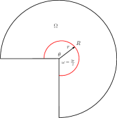
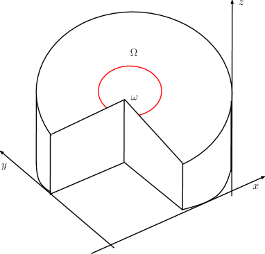
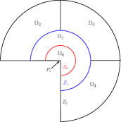
Figure 2: The domains, (a) two-dimensional with corner singularity, (b) three-dimensional with re-entrant edge, (c) subdivision of $\Omega$ into zones and subdomains.

3 IgA on graded meshes

In many realistic applications, we very often have to solve problems similar to (2.4) in domains with non-smooth boundary parts, that possess geometric singularities, for instance, non-convex corners, see Fig. 2. It is well-known that the numerical methods loose accuracy when they are applied to this type of problems. This occurs as a result of the reduced regularity of the solutions in the vicinity of the non-smooth parts [14]. When finite element methods are used, graded meshes have been utilized around the singular boundary parts in order to obtain optimal convergence rates, see e. g. [6, 3], see also [13] for dG methods. The basic idea of this grading mesh technique is to use the a priori knowledge of the singular behavior of the solution around the singular boundary points, cf. (2.7) and (2.6)), and consequently adjust accordingly the size of the elements.

The purpose of this paper is to extend the grading mesh techniques from the finite element method to dG IgA framework for solving boundary value problems like (2.4) in the presence of singular points. We develop a mesh grading algorithm around the singular boundary parts inspired by the grading mesh methodology using layers, therefore, extending the approach used in finite element methods, cf. [6, 5], to isogeometric analysis. Next, we construct the graded mesh and show that the proposed dG IgA method exhibits optimal convergence rates as for the problems with high regularity solutions. We present our mesh grading technique and the corresponding analysis for two-dimensional problems. In Section 4, we also apply our methodology to some three-dimensional examples and discuss the numerical results.

3.1 A priori mesh grading

The grading of the meshes around the singular points is guided by the exponent $\lambda$, which specifies the regularity of the function $u_{s}$, see (2.7), and by the location of the singular boundary point too. Next, we discuss the construction of the mesh for the case of one singular geometric point on $\partial\Omega$.

Let $P_{s}$ be the singular point and let $U_{s}:=\{x\in\Omega:|P_{s}-x|\leq R=L_{U}h,\;\mbox{with}\;L_{U}\geq 2\}$ be an area around $P_{s}$ in $\Omega$, which is further subdivided into $\zeta_{M}$ ring-type zones $Z_{\zeta}$, $\zeta=0,..,\zeta_{M}$, such that the distance from $P_{s}$ is $D_{(Z_{\zeta},P_{s})}:=C(n_{\zeta}h)^{\frac{1}{\mu}}$, where $C=R^{1-\frac{1}{\mu}}$ and $0\leq n_{\zeta}<L_{U}$. By $\mu\in(0,1]$, we denote the grading control parameter. The radius of every zone is defined to be $R_{Z_{\zeta}}:=D_{(Z_{\zeta+1},P_{s})}-D_{(Z_{\zeta},P_{s})}=C(n_{\zeta+1}h)^{\frac{1}{\mu}}-C(n_{\zeta}h)^{\frac{1}{\mu}}$, where we suppose that there is a $\nu>0$ such that $n_{\zeta+1}=n_{\zeta}+\nu$ with $1\leq\nu<L_{U}-1$. In particular, we set $R_{Z_{M}}=R-D_{(Z_{M-1},P_{s})}$.

For convenience, we assume that the initial subdivision $\mathcal{T}_{H}(\Omega)$ fits to the $Z_{\zeta}$ ring zone partition in order to fulfill the following conditions, for an illustration, see Fig. 2(c) with $\zeta_{M}=3$:

• The subdomains can be grouped into those which belong (entirely) into the area $U_{s}$ and those that belong (entirely) into $\Omega\setminus U_{s}$. This means that there is no $\Omega_{i},{\ }i=1,...,N$ such that $U_{s}\cap\Omega_{i}\neq\emptyset$ and $(\Omega\setminus U_{s})\cap\Omega_{i}\neq\emptyset$.

• Every ring zone $Z_{\zeta}$ is partitioned into “circular” subdomains $\Omega_{i_{\zeta}}$, which have radius $R_{\Omega_{i_{\zeta}}}$ equal to the radius of the zone, that is $R_{\Omega_{i_{\zeta}}}=R_{Z_{\zeta}}$. For computational efficiency reasons, we prefer, if it is possible, every zone to be only represented by one subdomain. This essentially depends on the characteristics of the problem, i.e., the shape of $\Omega$ and the coefficient $\alpha$.

• The zone $Z_{0}$ is represented by one subdomain, say $\Omega_{i_{0}}$, and the mesh $T^{({i_{0}})}_{h_{i_{0}}}(\Omega_{i_{0}})$ includes all the micro-elements $E$ such that $\partial E\cap P_{s}\neq\emptyset$.

We construct the meshes $T^{(i_{\zeta})}_{h_{i_{\zeta}}}(\Omega_{i_{\zeta}})$ (we will explain later how we can choose the grid size) in order to satisfy the following properties: for $\Omega_{i_{\zeta}}$ with distance $D_{(Z_{\zeta},P_{s})}$ from $P_{s}$, the mesh size $h_{i_{\zeta}}$ is defined to be $h_{i_{\zeta}}=\mathcal{O}(hR_{\Omega_{i_{\zeta}}}^{1-\mu})$ and for $T^{({i_{0}})}_{h_{i_{0}}}(\Omega_{i_{0}})$ the mesh size is of order $h_{i_{0}}=\mathcal{O}(h^{\frac{1}{\mu}}).$ Thus, we have the following relations:

$$C_{m}h^{\frac{1}{\mu}} \leq h_{{i_{\zeta}}}\leq C_{M}h^{\frac{1}{\mu}}, \text{if}{\ }\overline{\Omega}_{i_{\zeta}}\cap P_{s}\neq\emptyset,$$ (3.1a)

$$C_{m}hR_{\Omega_{i_{\zeta}}}^{1-\mu} \leq h_{i_{\zeta}}\leq C_{M}hD_{(Z_{\zeta},P_{s})}^{1-\mu}, \text{if}{\ }\overline{\Omega}_{i_{\zeta}}\cap P_{s}=\emptyset.$$ (3.1b)

We need to specify the mesh size for every $T^{({i_{\zeta}})}_{h_{i_{\zeta}}}(\Omega_{i_{\zeta}})$ in order to satisfy inequalities (3.1). We set the mesh size of $T^{({i_{\zeta}})}_{h_{i_{\zeta}}}(\Omega_{i_{\zeta}})$ to be of order $h_{i_{\zeta}}=\mathcal{O}(R_{Z_{\zeta}}\nu^{-(1/\mu}))$, and, for a uniform subdomain mesh, we can set

$$h_{i_{\zeta}}=C\frac{(n_{\zeta}+\nu)h)^{\frac{1}{\mu}}-(n_{\zeta}h)^{\frac{1}{\mu}}}{int(\nu^{\frac{1}{\mu}})}$$

where $C=R^{1-\frac{1}{\mu}}$ and $int(\nu^{-\mu})$ denotes the nearest integer to $\nu^{-\mu}$. Notice that the grading has “a subdomain character” and is mainly determined by the parameter $\mu\in(0,1]$. For $\mu=1$, we get $h_{i_{\zeta}}=h$, i.e., means we get quasi-uniform meshes. Using inequality $\mu\leq 1$ and inequality $(a+b)^{\gamma}\leq 2^{\gamma-1}(a^{\gamma}+b^{\gamma})$, which can easily be shown since the function $t^{\gamma}$ is convex in $(0,\infty)$, we arrive at the estimates

$$h_{i_{\zeta}} =C\frac{((n_{\zeta}+\nu)h)^{\frac{1}{\mu}}-(n_{\zeta}h)^{\frac{1}{\mu}}}{int(\nu^{\frac{1}{\mu}})}\leq C\frac{C_{\mu}(n_{\zeta}h)^{\frac{1}{\mu}}+C_{\mu}(\nu h)^{\frac{1}{\mu}}-(n_{\zeta}h)^{\frac{1}{\mu}}}{int(\nu^{\frac{1}{\mu}})}$$

$$\leq(C_{1,R,\mu,\nu}n_{\zeta})^{\frac{1}{\mu}}hh^{\frac{1}{\mu}-1}\leq\frac{(C_{1,R,\mu,\nu}n_{\zeta})^{\frac{1}{\mu}}}{n_{\zeta}^{\frac{1-\mu}{\mu}}}h\Big{(}\big{(}n_{\zeta}h\big{)}^{\frac{1}{\mu}}\Big{)}^{1-\mu}$$

$$\leq(C_{2,\mu,\nu}n_{\zeta})^{\frac{1}{\mu}}hD^{1-\mu}_{(Z_{\zeta},P_{s})},$$ (3.2)

which gives the right inequality in (3.1b). By the initial choice of $h_{i_{\zeta}}$, we have $h_{i_{\zeta}}=R_{\Omega_{i_{\zeta}}}/int(\nu^{-\mu})$. Since $1>1-\mu\geq 0$, we can easily show that

$$\frac{1}{int(\nu^{\frac{1}{\mu}})}R_{\Omega_{i_{\zeta}}}^{1-1+\mu}\geq C_{m}h,$$ (3.3)

with $C_{m}=\frac{1}{2}((n_{\zeta}+\nu)^{\frac{1}{\mu}}-n_{\zeta}^{\frac{1}{\mu}})$. From the choice grid sizes made above and (3.3), we can derive the left inequality in (3.1b).

Remark 2

It is possible to apply other techniques, see for example [6, 5], of constructing graded meshes, where we could prove optimal rates for the dG IgA method. We prefer the way that is described above for its simplicity and because it suits to the spirit of the dG IgA methodology.

3.2 Quasi-interpolant, error estimates

Next, we study the error estimates of the method (2.12). For the purposes of our analysis, we consider the enlarged space

$$W_{h}^{l,p}:=W^{1,2}(\Omega)\cap W^{l\geq 2,p}(\mathcal{T}_{H}(\Omega))+\mathbb{B}_{h}(\mathcal{T}_{H}(\Omega)),$$ (3.4)

where $p\in(\max\{1,\frac{2d}{d+2(l-1)}\},2]$. Let us mention that we allow different $l$ and $p$ in different subdomains $\Omega_{i}$. In particular, for subdomains ${\Omega}_{i}\cap U_{s}=\emptyset$, we can set in (3.4) $p=2$, for subdomains ${\Omega}_{i}\cap U_{s}\neq\emptyset$, we set $1<p=\frac{2}{2-\lambda}<2.$ The space $W_{h}^{1,2}$ is equipped with the broken dG-norm

$$\|u\|^{2}_{dG(\Omega)}=\sum_{i=1}^{N}\Big{(}\alpha^{(i)}\|\nabla u^{(i)}\|^{2}_{L^{2}(\Omega_{i})}+p_{i}(u^{(i)},u^{(i)})\Big{)},{\ }u\in W_{h}^{1,2}.$$ (3.5)

Let $f\in W^{1,2}(\Omega)\cap W^{l\geq 2,p}(\mathcal{T}_{H}(\Omega))$ with $p\in(\max\{1,\frac{2d}{d+2(l-1)}\},2]$, then we can construct a quasi-interpolant $\Pi_{h}f\in\mathbb{B}_{h}(\mathcal{T}_{H})$ such that $\Pi_{h}f=f$ for all $f\in\mathbb{B}_{h}(\mathcal{T}_{H})$. We refer to [28], see also [7], for more details about the construction of $\Pi_{h}f$. We have the following approximation estimate.

Lemma 1

Let $u\in W^{1,2}(\Omega)\cap W^{l,p}(\mathcal{T}_{H}(\Omega))$ with $p\in(\max\{1,\frac{2d}{d+2(l-1)}\},2]$ and $l\geq 2$, and let $E=\mathbf{\Phi}_{i}(\hat{E}),\hat{E}\in T^{(i)}_{h_{i},\hat{\Omega}}$. Then, for $0\leq m\leq l\leq k+1$, there exist an quasi-interpolant $\Pi_{h}u\in\mathbb{B}_{h}(\mathcal{T}_{H})$ and constants $C_{i}:=C_{i}\big{(}\max_{l_{0}\leq l}(\|D^{l_{0}}\mathbf{\Phi}_{i}\|_{L^{\infty}(\Omega_{i})})\big{)}$ such that

$$\sum_{E\in T^{(i)}_{h_{i},\Omega_{i}}}|u-\Pi_{h}u|^{p}_{W^{m,p}(E)}\leq C_{i}\|u\|_{W^{l,p}(\Omega_{i})}h_{i}^{p(l-m)}.$$ (3.6)

Furthermore, we have the following estimates in the $\|.\|_{dG(\Omega)}$ norm

$$\|u-\Pi_{h}u\|_{dG(\Omega)}\leq \sum_{i=1}^{N}C_{i}\Big{(}h_{i}^{\delta(l,p,d)}\|u\|_{W^{l,p}(\Omega_{i})}\Big{)}+$$ (3.7a)

$$\qquad\sum_{i=1}^{N}\sum_{F_{ij}\subset\partial\Omega_{i}}C_{i}\alpha^{(j)}\frac{h_{i}}{h_{j}}\Big{(}h_{i}^{\delta(l,p,d)}\|u\|_{W^{l,p}(\Omega_{i})}\Big{)},$$

$$\|u_{h}-\Pi_{h}u\|_{dG(\Omega)}\leq \|u-\Pi_{h}u\|_{dG(\Omega)}+\sum_{i=1}^{N}C_{i}h_{i}^{\delta(l,p,d)}\|u\|_{W^{l,p}(\Omega_{i})},$$ (3.7b)

where $\delta(l,p,d)=l+(\frac{d}{2}-\frac{d}{p}-1)$.

Proof

The proof is given in [24]. $\Square$

Remark 3

If $h_{i}$ and $h_{j}$ are the grid sizes of two adjacent subdomains $\Omega_{i}$ and $\Omega_{j}$, then relations (3.1) immediately yield the two-side estimate $\sigma_{m,\zeta}\leq{h_{i}}/{h_{j}}\leq\sigma_{M,\zeta}$, where the positive constants $\sigma_{m,\zeta}$ and $\sigma_{M,\zeta}$ only depend on the quantities which specify the initial zone partition $Z_{\zeta}$. Hence, in what follows, estimate (3.7a) will be used in the form $\|u-\Pi_{h}u\|_{dG(\Omega)}\leq\sum_{i=1}^{N}C_{i}h_{i}^{\delta(l,p,d)}$. We mention that the analysis presented here can easily be extended to non-matching grids, see [24]. We also note that the meshes $T^{({i_{\zeta}})}_{h_{i_{\zeta}}}(\Omega_{i_{\zeta}})$ satisfy the Assumption 1.

We emphasize that Lemma 1 provides local estimates which hold in every subdomain $\Omega_{i}$. This help us to investigate the accuracy of the method in every zone $Z_{\zeta}$ of $U_{s}$ separately. We give an approximation estimate for the case where $u_{r}\in W^{l,2}(\Omega)$ with $l\geq k+1$, see (2.6).

For all $\Omega_{i_{\zeta}}\in Z_{\zeta}$, the local interpolation estimate (3.7a) gives

$$\|u_{s}-\Pi_{h}u_{s}\|_{dG(U_{s})}\leq\sum_{{i_{\zeta}}}h_{{i_{\zeta}}}^{\lambda}C_{{i_{\zeta}}},$$ (3.8)

since $u_{s}\in W^{l=2,p=\frac{2}{2-\lambda}}(\Omega)$.

Theorem 3.1

Let $Z_{\zeta}$ be a zone partition of $\Omega$ with the properties listed in the previous section, and let $T_{h_{i}}^{(i)}(\Omega_{i})$ be the meshes of the subdomains as described in Section 3.1. Then, for the solution $u$ of (2.4a), we have the error estimate

$$\|u-u_{h}\|_{dG(\Omega)}\leq h^{r}C,\quad\text{with}\;r=\min\{k,{\lambda}/{\mu}\},$$ (3.9)

where the constant $C>0$ is determined by the quasi uniform mesh properties, see (3.1), and the constants $C_{i}$ of Lemma 1.

Proof

Let $\Pi_{h}u\in\mathbb{B}_{h}(\mathcal{T}_{H})$ be the quasi-interpolant of Lemma 1. Using the triangle inequality, we obtain

$$\|u-u_{h}\|_{dG(\Omega)}\leq\|u_{h}-\Pi_{h}u\|_{dG(\Omega)}+\|u-\Pi_{h}u\|_{dG(\Omega)}.$$ (3.10)

Moreover, representation (2.6) yields

$$\|u-\Pi_{h}u\|_{dG(\Omega)}\leq\|u_{s}-\Pi_{h}u_{s}\|_{dG(\Omega)}+\|u_{r}-\Pi_{h}u_{r}\|_{dG(\Omega)}.$$ (3.11)

Using the fact that $u_{r}\in W^{l\geq k+1,2}(\Omega)$, Lemma 1, the mesh properties (3.1) and inequalities $0<\mu\leq 1$, we have

$$\|u_{r}-\Pi_{h}u_{r}\|_{dG(\Omega)}\leq C_{1}h^{\frac{k}{\mu}}+C_{2}h^{k}\leq Ch^{k},$$ (3.12)

where the constants $C_{1}$ and $C_{2}$ are determined by the constants that appear in (3.1) and (3.7a). Therefore, it remains to estimate the first term in (3.11). By (3.1a) and (3.8), we obtain the estimate

$$\|u_{s}-\Pi_{h}u_{s}\|_{dG(Z_{0})}\leq Ch_{i_{0}}^{\lambda}\leq Ch^{\frac{\lambda}{\mu}}$$ (3.13)

in $Z_{0}$, where the constant $C$ is determined by the constants in (3.1) and (3.7a). For the subdomains belonging to the remaining zones of $Z_{\zeta},{\ }\zeta\neq 0$, (3.1b) and (3.8) yield the estimates

$$\|u_{s}-\Pi_{h}u_{s}\|_{dG(Z_{\zeta})} \leq C_{\zeta\neq 0}h_{i_{\zeta}}^{\lambda}\leq C_{\zeta\neq 0}\big{(}hD^{1-\mu}_{(Z_{\zeta},P_{s})}\big{)}^{\lambda}$$

$$\leq C_{\zeta\neq 0}\big{(}hh^{\frac{1-\mu}{\mu}}\big{)}^{\lambda}\leq C_{\zeta\neq 0}h^{\frac{\lambda}{\mu}}.$$ (3.14)

Collecting (3.12), (3.13) and (3.2), we arrive at the interpolation error estimate

$$\|u-\Pi_{h}u\|_{dG(\Omega)}\leq Ch^{r},$$ (3.15)

with $r=\min\{k,{\lambda}/{\mu}\}$. Now, inserting estimate (3.15) into (3.10) and recalling estimate (3.7b), we can easily derive the error estimate (3.9). $\Square$

4 Numerical examples

In this section, we present a series of numerical examples in order to confirm the theoretical results and to assess the effectiveness of the proposed grading mesh technique. The first examples concern two-dimensional problems with boundary point singularities and with highly discontinuous coefficients. In the last examples, we consider applications of the method to three-dimensional problems with an interior singularity and in domains with singular edges having $\omega=3\pi/2$ interior angle. The numerical examples have been performed in G+Smo .

4.1 Implementation details

The grading of the mesh is done in the parameter domain. The underlying assumption is that the given parameterization of the domain has uniform speed along the patch. An ideal situation is to have an arc-length parameterization. Nevertheless, a well-behaving parameterization is one whose speed is within a constant factor of the arc-length parameterization. This is a reasonable assumption, also because CAD software typically try to adhere to such a requirement, since it is desirable for CAD operations as well.

For constructing the graded parameter mesh, we choose a number of interior knots in each parametric direction and we place the knots according to the grading parameter and the location of the singular point in parameter space. In Fig. 3(a), we show the one-dimensional B-spline basis on a graded mesh, and similarly in In Fig. 3(b), we present the two- dimensional B-spline basis on the corresponding graded mesh. If the location of the singular point is given in physical coordinates, we invert the point to parameter space with a Newton iteration, to map it back to parameter space.

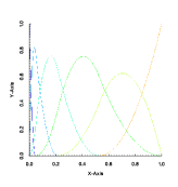
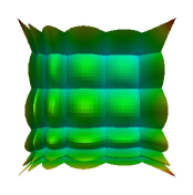
Figure 3: Basis functions on the graded mesh $T^{(i_{\zeta})}_{h_{i_{\zeta}},\widehat{\Omega}}$: (a) The 1d bases on $\mu=0.6$ grading, (b) The 2D bases on $\mu=0.6$ grading.

Under the assumption of a well-behaved B-spline geometry map, the parameter mesh is transformed from $T^{(i_{\zeta})}_{h_{i_{\zeta}},\widehat{\Omega}}$ to $T^{(i)}_{h_{i},\Omega_{i}}$ in such a way that the size of the physical elements are proportional to their (pre-image) parametric elements. This property ensures that our theoretical analysis applies in the experiments that we conducted.

For efficiency reasons, the mesh $\mathcal{T}_{H}(\Omega)$ is created by the grading function with the same number of knots as an equivalent uniform mesh with grid size $h_{i}$ for each subdomain $\Omega_{i}$, but pulled towards the singularity $P_{s}$ using the grading parameter $\mu$. This strategy satisfies Assumption 1 with a minimal number of knots. This approach also mimics the zones construction introduced in Subsection 3.1, since it corresponds to a zone partition that shrinks towards $P_{s}$ at every refinement step.

In our experiments, we consider a mapping $\mathbf{\Phi}_{i}$ produced on an initial knot vector $\mathbf{\Xi}_{i}^{d}$, which exactly represents the subdomain $\Omega_{i}$, as the isogeometric paradigm suggests. The knots are relocated during the grading procedure but without changing the shape or the parameterization of the subdomains $\Omega_{i}$. If needed, the original coarse knots are inserted in the discretization basis such that the exact representation of the original shape is feasible. Nevertheless, in our implementation, we have the freedom to use a different sequence of knots for the discretization space without refining the initial geometry in this basis.

4.2 Numerical Examples for Two dimensional

4.2.1 Heart shaped domain

To illustrate the efficiency of the proposed mesh grading methodology and to validate the estimates of Section 2, we consider the problem (2.4) in a curved domain (heart shape) having a singular point $P_{s}$ (re-entrant corner) with internal angle $\omega=3\pi/2$, see Fig. 4(a).

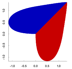
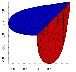
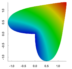
Figure 4: Heart shape problem: (a) the computational domain and the subdomains, (b) the graded meshes of the two subdomains, (c) the contours of $u_{h}$ solution.

$j_{1}$	$j_{2}$	$B^{1}_{j}(j_{1},j_{2})$	$B^{2}_{j}(j_{1},j_{2})$
$1$	$1$	$(0.00,0.00)$	$(0.00,0.00)$
$2$	$1$	$(0.49,0.49)$	$(0.49,0.49)$
$3$	$1$	$(0.97,0.97)$	$(0.97,0.97)$
$1$	$2$	$(0.00,-0.81)$	$(-0.81,0.00)$
$2$	$2$	$(0.46,-0.16)$	$(-0.16,0.46)$
$3$	$2$	$(1.00,0.94)$	$(0.94,1.00)$
$1$	$3$	$(0.35,-0.84)$	$(-0.84,0.35)$
$2$	$3$	$(0.71,-0.84)$	$(-0.84,0.71)$
$3$	$3$	$(0.85,0.042)$	$(0.04,0.85)$

Table 1: The control points for the two B-spline surfaces each with degree $k=2$ depicted in Figure 4

	without grading		with grading
$h/2^{s}$	$k=1$	$k=2$	$\begin{matrix}k=1,\\ \mu=0.6\end{matrix}$	$\begin{matrix}k=2,\\ \mu=0.3\end{matrix}$
Convergence rates
$s=0$	-	-	-	-
$s=1$	0.671469	0.68221	0.843026	1.49519
$s=2$	0.678694	0.67322	0.894636	1.85785
$s=3$	0.677558	0.669385	0.921219	2.02913
$s=4$	0.675018	0.667797	0.938709	2.02562
$s=5$	0.672622	0.667156	0.951475	2.00987

Table 2: Heart shape problem: The convergence rates in the dG-norm $\|.\|_{dg(\Omega)}$ with and without grading.

The computational domain $\Omega$ consists of two subdomains shown in Fig. 4(a), where the corresponding knot vectors are $\mathbf{\Xi}_{i}^{2}=(\Xi_{i}^{1},\Xi_{i}^{2}),i=1,2$ with $\Xi_{i}^{1}=\Xi_{i}^{2}=\{0,0,0,1,1,1\}$ and are parametrized by $k=2$ B-spline basis with the control points given in Table 1. The exact solution is given by $u=r^{\frac{\pi}{\omega}}\sin(\theta\pi/\omega)$ with $f$ and $u_{D}$ in (2.4) are specified by the exact solution. We set $\alpha=1$ in the entire $\Omega$. Note that $u\in W^{1.5,2}(\Omega)$. The problem has been solved using first ($k=1$) and second ($k=2$) order B-spline spaces with grading parameter $\mu=0.6$ and $\mu=0.3$, respectively, see Fig. 4(b). We plot the contours of the solution $u_{h}$ computed using $k=2$ B-splines in Figure 4(c). In Table 2, we display the convergence rate of the error. In the left column (without grading), we present the rates using quasi-uniform meshes. In the right column of the table, we show the rates in the case of using graded meshes. As the theory predicts, the convergence rates in left columns of both cases $k=1$ and $k=2$ are mainly determined by the regularity of the solution. One the other hand, the rates which correspond to the graded meshes tend to be optimal with respect to the B-spline degree $k$. This shows the adequacy of the proposed graded mesh for solving this problem.

4.2.2 Kellogg’s Problem.

It is known that the solutions of problem (2.4) with rough diffusion coefficients may not be very smooth. Thus, standard numerical method can not provide an (optimal) accurate approximation [12]. We examine such a case by solving the so-called Kellogg test problem [18]. We consider the computational domain $\Omega=(-1,1)^{2}$. The diffusion coefficient $\alpha$ in (2.3) is supposed to be piecewise constant taking the same value, say $\alpha:=\alpha_{13}$, in the first and third quadrants, and, similarly, for the second and fourth quadrants, $\alpha:=\alpha_{24}$.

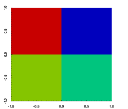
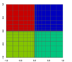
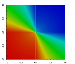
Figure 5: Kellogg’s test problem: (a) The computational domain and the four subdomains, (b) the graded meshes of the four subdomains, (c) the contours of $u_{h}$ solution.

This choice of the diffusion coefficient leads to the subdivision of $\Omega$ in the four subdomains as it is shown in Fig. 5(a). The exact solution of the problem for $f=0$ is given in polar coordinates by $u(r,\theta)=r^{\lambda}\varphi(\theta)$, where

$$\varphi(\theta)=\begin{cases}\cos((\pi/2-\sigma)\lambda)\cos((\theta-\pi/2+\rho)\lambda),&\text{if }0\leq\theta<\pi/2,\\ \cos(\rho\lambda)\cos((\theta-\pi+\sigma)\lambda),&\text{if }\pi/2\leq\theta<\pi,\\ \cos(\sigma\lambda)\cos((\theta-\pi-\rho)\lambda),&\text{if }\pi\leq\theta<3\pi/2,\\ \cos((\pi/2-\rho)\lambda)\cos((\theta-3\pi/2-\sigma)\lambda),&\text{if }3\pi/2\leq\theta\leq 2\pi,\\ \end{cases}$$

where the numbers $\lambda,\rho,\sigma$ satisfy the nonlinear relations

$$\begin{cases}\mathcal{R}:=\frac{\alpha_{13}}{\alpha_{24}}=-\tan((\pi/2-\sigma)\lambda)\cot(\rho\lambda),\\ \frac{1}{\mathcal{R}}=-\tan(\rho\lambda)\cot(\sigma\lambda),\\ \mathcal{R}=-\tan(\sigma\lambda)\cot((\pi/2-\rho)\lambda),\\ 0<\lambda<2,\\ \max\{0,\pi\lambda-\pi\}<2\lambda\rho<\min\{\pi\lambda,\pi\},\\ \max\{0,\pi-\pi\lambda\}<-2\lambda\sigma<\min\{\pi,2\pi-\lambda\pi\}.\end{cases}$$

For $\lambda=0.4$, the solution $u\in W^{1.4,2}(\Omega)$, and has discontinuous derivatives across the interfaces. On the other hand, $u\in W^{2,1.25}(\Omega)$, and the estimates presented in Section 3.3 can be applied. We solved the problem using B-spline spaces with degrees $k=1$ and $k=2$ on uniform meshes. We performed again the test using graded meshes with grading parameter chosen such that $\lambda/\mu=k$, see (3.9). In Fig. 5(b), we can see the graded meshes of the subdomains. Fig. 5(c) shows the plot of the contours of the dG solution $u_{h}$ computed for degree $k=1$ B-splines. In Table 3, we display the convergence rates of the solution. We observe that, in the case of uniform meshes, the experimental order of convergence of the method is $0.4$ which is determined by the regularity of the solution. Conversely, the rates in the right columns which correspond to the results using mesh grading tend to be optimal with respect the order of the B-spline space.

	without grading		with grading
$h/2^{s}$	$k=1$	$k=2$	$\begin{matrix}k=1,\\ \mu=0.40\end{matrix}$	$\begin{matrix}k=2,\\ \mu=0.20\end{matrix}$
Convergence rates
$s=0$	-	-	-	-
$s=1$	0.655814	0.591165	0.830217	0.477657
$s=2$	0.354865	0.355586	0.858329	1.15442
$s=3$	0.368103	0.378796	0.879976	1.78696
$s=4$	0.378375	0.385672	0.895984	1.84425
$s=5$	0.385464	0.390348	0.906179	1.95223

Table 3: Kellogg’s test: The convergence rates in the dG-norm $\|.\|_{dg(\Omega)}$.

A glimpse of the discrete solution $u_{h}$ is given in Fig. 6.

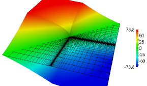
Figure 6: Discrete solution of Kellogg’s problem plotted over the graded mesh.

4.3 Three dimensional examples

4.3.1 Cube with interior point singularity.

This test case is inspired by [21]. The computational domain is $\Omega=(-1,1)^{3}$ which is decomposed into 8 subdomains, see Fig. 7(a). We choose the diffusion coefficient $\alpha=1$ in the whole computational domain $\Omega$. The solution of the problem has a singular point at the origin of the axis and is given by $u(x)=|x|^{\lambda}$ with $\lambda=0.85$. It is easy to show that $u\in W^{l=2,2}(\Omega)$. We solved the problem using $k=1,{\ }k=2$ and $k=3$ B-spline spaces on quasi-uniform meshes. In Fig. 7(b), we plot the contours of solution $u_{h}$ computed by $k=1$ B-spline space. The convergence rates of the error corresponding to non-graded meshes are shown in left columns of Table 4.

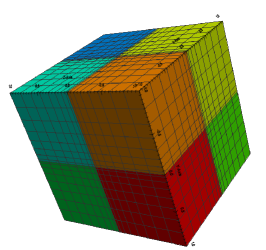
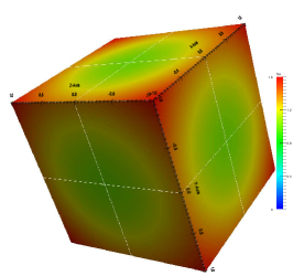
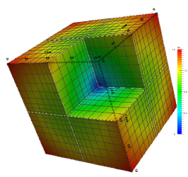
Figure 7: Cube with interior singularity: (a) the decomposition of $\Omega$ into 8 subdomains with the graded meshes of the subdomain, (b) the contours of the solution $u_{h}$, (c) the variance of the $u_{h}$ contours around the singular point.

The rates are optimal for $k=1$ B-spline space and sub-optimal for the two other B-spline spaces, as it was expected according to the regularity of the solution $u$. Note that the rates presented on the left columns in Table 4 are in agreement with the estimate given in (3.7a). We have performed again the test using grading meshes for the last two B-spline spaces. The grading parameter $\mu$ has been chosen to be $\delta(l=2,p=2,d=3)/\mu=k$, see Lemma 1 and (3.9). In Fig. 7(c), the variate of the $u_{h}$ contours around the singular point is shown. The rates obtained on graded meshes are displayed in right columns of Table 4.

	without grading			with grading
$h/2^{s}$	$k=1$	$k=2$	$k=3$	$\begin{matrix}k=1,\\ \mu=1.0\end{matrix}$	$\begin{matrix}k=2,\\ \mu=0.6\end{matrix}$	$\begin{matrix}k=3,\\ \mu=0.4\end{matrix}$
Convergence rates
$s=0$	-	-	-	-	-	-
$s=1$	0.593	1.066	0.687	0.593	1.393	0.791
$s=2$	0.839	1.306	1.234	0.839	1.766	1.870
$s=3$	0.917	1.340	1.343	0.917	1.928	2.942
$s=4$	0.953	1.346	1.350	0.953	1.959	3.080
$s=5$	0.972	1.348	1.350	0.972	1.974	3.066

Table 4: Cube with interior singularity: The convergence rate of the error on uniform and graded meshes.

We can observe that the rates approach the optimal rate for both high-order B-spline spaces. This numerical example demonstrates that the dG IgA method applied on the proposed graded meshes can exhibit optimal convergence rates for interior singularity type problems as well.

4.3.2 Three-dimensional L-shape domain.

Now the computational domain $\Omega$ has 3d L-shape form and is given by $\left((-1,1)^{2}\setminus(-1,0)^{2}\right)\times[0,1]$. Even though the ”L-shape“ example has been mostly studied in the literature in its two-dimensional set up, (see for example anisotropic 2d meshes for IgA discretizations in [8]), we believe that it is an interesting test case, because we will see that the graded mesh of the plane can be prolonged in a direction perpendicular to the singular edge for treating the boundary singularities. Note that in this three dimensional setting, the domain includes both corner and edge singularities, see Fig. 8(a).

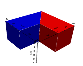
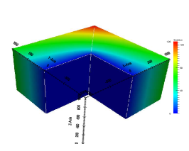
Figure 8: 3d L-shape test: (a) The domain $\Omega$ with the corners and the edge boundary singularities, (b) The graded meshes of the two subdomain, (c) The contours of $u_{h}$.

We consider an exact solution given by $u=r^{\lambda}\sin(\frac{\theta\pi}{\omega}),$ where $\lambda=\pi/\omega$ and $\omega=3\pi/2$. We set $\Gamma_{D}=\partial\Omega$. The data ${f}$ and ${u}_{D}$ of (2.3) are given by the exact solution. The computational domain $\Omega$ consists of two subdomains We have solved the problem using B-spline spaces of order $k=1$ and $k=2$ using quasi-uniform and graded meshes in both subdomains. The grading parameter is defined by the relation $\delta(l,p,d)/\mu=k$. In Fig. 8(b), we can see the graded meshes for $\mu=0.6$. The contours of the corresponding approximate solution $u_{h}$ computed for $k=1$ are presented in Fig. 8(c). Table 5 displays the convergence rates of the error. We observe the same behavior of the rates as in the previous examples. The rates of the uniform meshes are determined by the regularity of the solution ($u\in W^{1+\lambda,p=2}(\Omega)$) for both B-spline spaces. The convergence rates corresponding to graded meshes approach the optimal value. We remark here that the same type of graded meshes have also been used in finite element methods for approximating solutions of elliptic problems in three-dimensional domains with edges, see [6, 5, 4].

	without grading		with grading
$h/2^{s}$	$k=1$	$k=2$	$\begin{matrix}k=1,\\ \mu=0.6\end{matrix}$	$\begin{matrix}k=2,\\ \mu=0.3\end{matrix}$
Convergence rates
$s=0$	-	-	-	-
$s=1$	0.645078	0.477178	0.629909	0.387338
$s=2$	0.650805	0.639951	0.869128	1.11198
$s=3$	0.642971	0.670841	0.883655	1.80531
$s=4$	0.644107	0.669949	0.902467	1.96533
$s=5$	0.648100	0.668371	0.920065	2.00296

Table 5: 3d L-shape : The convergence rates of the error with respect to the dG norm on uniform and graded meshes.

4.3.3 Three-dimensional heart shaped domain.

In this example, we consider an exact solution given by $u=r^{\lambda}\sin(\theta\pi/\omega),$ where $\lambda=\pi/\omega$ and $\omega=3\pi/2$. We again set $\Gamma_{D}=\partial\Omega$, and the data ${f}$ and ${u}_{D}$ of (2.3) are specified by the given exact solution. The computational domain $\Omega$ consists of two subdomains. The problem is solved with B-spline spaces of order $k=1$ and $k=2$ using quasi-uniform and graded meshes in both subdomains. The grading parameter is defined by the relation $\lambda/\mu=k$. In Fig. 9(b), we can see the graded meshes for $\mu=0.6.$ The contours of the corresponding approximate solution $u_{h}$ computed with degree $k=1$ is presented in Fig. 9(c).

The convergence rates of the error corresponding to the quasi-uniform meshes are shown in left columns (without grading) of Table 6, and the rates corresponding to the graded meshes are shown in the right columns of Table 6.

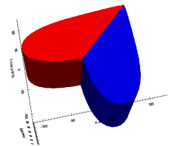
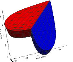
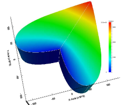
Figure 9: 3D heart test: (a) The domain $\Omega$ with the corners and edge boundary singularities, (b) The graded meshes of the two subdomain, (c) The contours of $u_{h}$.

	without grading		with grading
$h/2^{s}$	$k=1$	$k=2$	$\begin{matrix}k=1,\\ \mu=0.6\end{matrix}$	$\begin{matrix}k=2,\\ \mu=0.3\end{matrix}$
Convergence rates
$s=0$	-	-	-	-
$s=1$	0.650805	0.675611	0.686633	0.964287
$s=2$	0.642971	0.685756	0.846524	1.55143
$s=3$	0.644107	0.674337	0.902119	1.91781
$s=4$	0.6481	0.669817	0.925762	2.10561
$s=5$	0.65251	0.667968	0.94134	2.09457

Table 6: 3d Heart : The convergence rates of the error with respect to the dG norm on uniform and graded meshes.

5 Conclusion

We have presented mesh grading techniques for dG IgA discretizions of elliptic boundary value problems in the presence of so-called singular points. Based on the a priori or a posteriori knowledge of the behaviour of the exact solution around the singular points, we pre-defined the grading of the mesh without increasing the knots but performing a relocation. The grading refinement has a subdomain (patch) character in order to fit well into the IgA framework. Optimal error estimates of the multipatch dG IgA method have been shown when it is used on the graded meshes proposed. The theoretical results have been confirmed by a number of two- and three-dimensional test problems with known exact solutions.

Acknowledgment

This research was supported by the National Research Network NFN S117-03 “Geometry + Simulation” of the Austrian Science Fund (FWF).

References

- [1] R. A. Adams and J. J. F. Fournier. Sobolev Spaces, volume 140 of Pure and Applied Mathematics. ACADEMIC PRESS-imprint Elsevier Science, second edition, 2003.
- [2] T. Apel. Interpolation of non-smooth functions on anisotropic finite element meshes. M2AN, 33(6):1149–1185, 1999.
- [3] T. Apel and B. Heinrich. Mesh refinement and windowing near edges for some elliptic problem. SIAM J. Numer. Anal., 31(3):695–708, 1994.
- [4] T. Apel and B. Heinrich. The finite element method with anisotropic mesh grading for elliptic problems in domains with corner and edges. SIAM J. Numer. Anal., 31(3):695–708, 1998.
- [5] T. Apel and F. Milde. Comparison of several mesh refinement strategies near edges. Comm. Num. Meth. Eng., 12:373–381, 1996.
- [6] T. Apel, A.-M. Sändig, and J. R. Whiteman. Graded mesh refinement and error estimates for finite element solutions of elliptic boundary value problems in non-smooth domains. Math. Methods Appl. Sci., 19(30):63–85, 1996.
- [7] Y. Bazilevs, L. Beirão da Veiga, J. Cottrell, T. Hughes, and G. Sangalli. Isogeometric analysis: Approximation, stability and error estimates for -refined meshes. M3AS, 16(07):1031–1090, 2006.
- [8] L. Beirão da Veiga, D. Cho, and G. Sangalli. Anisotropic NURBS approximation in isogeometric analysis. Comp. Methods in Appl. Mech and Engrg, 209–212(0):1 – 11, 2012.
- [9] J. A. Cottrell, T. J. R. Hughes, and Y. Bazilevs. Isogeometric Analysis, Toward Integration of CAD and FEA. John Wiley and Sons, 2009.
- [10] D. A. Di Pietro and A. Ern. Mathematical Aspects of Discontinuous Galerkin Methods, volume 69 of Mathématiques et Applications. Springer-Verlag, Heidelberg, Dordrecht, London, New York, 2012.
- [11] M. Dryja. On discontinuous Galerkin methods for elliptic problems with discontinuous coeffcients. Comput. Methods Appl. Math., 3:76–85, 2003.
- [12] S. R. Falkand and J. E. Osborn. Remarks on mixed finite element methods for problems with rough coefficients. Math. Comp., 62(205):1–19, 1994.
- [13] M. Feistauer and A.-M. Sändig. Graded mesh refinement and error estimates of higher order for dgfe solutions of elliptic boundary value problems in polygons. Numer. Methods Partial Diff. Equations, 28(4):1124–1151, 2012.
- [14] P. Grisvard. Elliptic problems in nonsmooth domains. Monographs and studies in mathematics. Pitman Advanced Pub. Program, 1985.
- [15] P. Grisvard. Singularities in Boundary Value Problems. Recherches en mathématiques appliquées. Masson, 1992.
- [16] T. Hughes, J. Cottrell, and Y. Bazilevs. Isogeometric analysis: CAD, finite elements, NURBS, exact geometry and mesh refinement. Comput. Methods Appl. Mech. Engrg., 194:4135–4195, 2005.
- [17] J. W. Jeong, H. S. Oh, S. K., and H. Kim. Mapping techniques for isogeometric analysis of elliptic boundary value problems containing singularities. Comp. Methods in Appl. Mech and Engrg, 254(0):334 – 352, 2013.
- [18] R. B. Kellogg. On the Poisson equation with intersecting interfaces. Appl. Anal., 4:101–129, 1975.
- [19] V. A. Kondrat’ev. Boundary value problems for elliptic equations in domains with conical or angular points. Transl. Moscow Math. Soc., 16:227–313, 1967.
- [20] V. Kozlov, V. G. Maz’ya, and J. Rossmann. Spectral Problems Associated with Corner Singularities of Solutions to Elliptic Equations, volume 85 of Mathematical Surveys and Monographs. Americanb Mathematical Society, Rhode Issland, USA, 2001.
- [21] D. Kröner, M. Růžička, and I. Toulopoulos. Numerical solutions of systems with -structure using local discontinuous Galerkin finite element methods. Int. J. Numer. Methods Fluids, 2014.
- [22] U. Langer, A. Mantzaflaris, S. Moore, and I. Toulopoulos. Multipatch discontinuous Galerkin Isogeometric Analysis. RICAM Reports 2014-18, Johann Radon Institute for Computational and Applied Mathematics, Austrian Academy of Sciences, Linz, 2014. http://arxiv.org/abs/1411.2478v1.
- [23] U. Langer and S. Moore. Discontinuous Galerkin isogeometric analysis of elliptic PDEs on surfaces. NFN Technical Report 12, Johannes Kepler University Linz, NFN Geometry and Simulation, Linz, 2014. http://arxiv.org/abs/1402.1185 and accepted for publication in the DD22 proceedings.
- [24] U. Langer and I. Toulopoulos. Analysis of multipatch discontinuous Galerkin IgA approximations to elliptic boundary value problems. RICAM Reports 2014-08, Johann Radon Institute for Computational and Applied Mathematics, Austrian Academy of Sciences, Linz, 2014. http://arxiv.org/abs/1408.0182.
- [25] L. Oganesjan and L. Ruchovetz. Variational Difference Methods for the Solution of Elliptic Equations. Isdatelstvo Akademi Nank Armjanskoj SSR, Erevan, 1979. (in Russian).
- [26] H. S. Oh, H. Kim, and J. W. Jeong. Enriched isogeometric analysis of elliptic boundary value problems in domains with cracks and/or corners. Int. J. Numer. Meth. Engn, 97(3):149–180, 2014.
- [27] B. Rivière. Discontinuous Galerkin Methods for Solving Elliptic and Parabolic Equations: Theory and Implementation. SIAM, Philadelphia, 2008.
- [28] L. L. Schumaker. Spline Functions: Basic Theory. Cambridge, University Press, 3rd edition, 2007.
- [29] G. Strang and G. Fix. An Analysis of the Finite Element Method. Prentice-Hall. Englewood Cliffs, N.J., 1973.