Hankel determinants for a singular complex weight and the first and third Painlevé transcendents

Abstract

In this paper, we consider polynomials orthogonal with respect to a varying perturbed Laguerre weight $e^{-n(z-\log z+t/z)}$ for $t<0$ and $z$ on certain contours in the complex plane. When the parameters $n$, $t$ and the degree $k$ are fixed, the Hankel determinant for the singular complex weight is shown to be the isomonodromy $\tau$-function of the Painlevé III equation. When the degree $k=n$, $n$ is large and $t$ is close to a critical value, inspired by the study of the Wigner time delay in quantum transport, we show that the double scaling asymptotic behaviors of the recurrence coefficients and the Hankel determinant are described in terms of a Boutroux tronquée solution to the Painlevé I equation. Our approach is based on the Deift-Zhou nonlinear steepest descent method for Riemann-Hilbert problems.

2010 Mathematics Subject Classification: Primary 33E17, 34M55, 41A60.

Keywords and phrases: Asymptotics; Hankel determinants; Painlevé I equation; Painlevé III equation; Riemann-Hilbert approach.

1 Introduction and statement of results

Let $w_{t}(x)$ be the following singularly perturbed Laguerre weight

$$w_{t}(x)=w(x;t)=e^{-nV_{t}(x)},\qquad x\in(0,+\infty)$$ (1.1)

with

$$V_{t}(x)=x-\log x+\frac{t}{x},~{}~{}t\geq 0.$$ (1.2)

The Hankel determinant is defined as

$$D_{k}[w(x;t)]=\det(\mu_{i+j})_{i,j=0}^{k-1},$$ (1.3)

where $\mu_{j}$ is the $j$-th moment of $w_{t}(x)$, namely,

$$\mu_{j}=\int_{0}^{\infty}x^{j}w_{t}(x)dx.$$

Note that when $t\geq 0$, the integral in the above formula is convergent so that the Hankel determinant $D_{k}[w;t]=D_{k}[w(x;t)]$ in (1.3) is well-defined. Moreover, it is well-known that the Hankel determinant can be expressed as

$$D_{k}[w;t]=\prod_{j=0}^{k-1}\gamma_{j,n}^{-2}(t);$$ (1.4)

see [26, p.28], where $\gamma_{k,n}(t)$ is the leading coefficient of the $k$-th order polynomial orthonormal with respect to the weight function in (1.1). Or, let $\pi_{k,n}(x)$ be the $k$-th order monic orthogonal polynomial, then $\gamma_{k,n}(t)$ appears in the following orthogonal relation

$$\int_{0}^{\infty}\pi_{k,n}(x)x^{j}e^{-nV_{t}(x)}dx=\gamma_{k,n}^{-2}(t)\delta_{jk},\qquad j=0,1,\cdots,k$$

for fixed $n$. Moreover, the monic orthogonal polynomials $\pi_{k,n}(x)$ satisfy a three-term recurrence relation as follows:

$$x\pi_{k,n}(x)=\pi_{k+1,n}(x)+\alpha_{k,n}(t)\pi_{k,n}(x)+\beta_{k,n}(t)\pi_{k-1,n}(x),~{}~{}k=0,1,\cdots,$$ (1.5)

with $\pi_{-1,n}(x)\equiv 0$ and $\pi_{0,n}(x)\equiv 1$, where the appearance of $n$ and $t$ in the coefficients indicates their dependence on $n$ and the parameter $t$ in the varying weight (1.1).

In this paper, however, we will focus on the case when $t<0$. Since all the above integrals on $[0,\infty)$ become divergent for negative $t$, we need to deform the integration path from the positive real axis to certain curves in the complex plane. Consequently, the orthogonality will be converted to the non-Hermitian orthogonality in the complex plane. More precisely, let us define the following new weight function on $\Gamma=\Gamma_{1}\cup\Gamma_{2}\cup\Gamma_{3}$:

$$w_{t}(z)=w(z;t)=c_{j}e^{-nV_{t}(z)},~{}~{}z\in\Gamma_{j},~{}~{}\textrm{with}~{}c_{1}=1,c_{2}=\alpha,c_{3}=1-\alpha,$$ (1.6)

where $\alpha$ is a complex constant, the curves $\Gamma_{1}=(2\delta,\infty)$, $\Gamma_{2}=\{\delta(1+e^{i\theta})|\;\theta\in(0,\pi)\}$ and $\Gamma_{3}=\{\delta(1+e^{i\theta})|\;\theta\in(-\pi,0)\}$; see Figure 1, $\delta$ being a positive constant. The potential is defined in the cut plane $\mathbb{C}\setminus(-\infty,0]$ as

$$V_{t}(z)=z-\log z+\frac{t}{z},~{}~{}\arg z\in(-\pi,\pi),~{}~{}t<0.$$ (1.7)

The orthogonality relation now takes the form

$$\int_{\Gamma}\pi_{k,n}(z)z^{j}w_{t}(z)dz=\gamma_{k,n}^{-2}(t)\delta_{jk},~{}~{}j=0,1,\cdots,k.$$ (1.8)

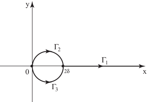
Figure 1: Contour of orthogonality, $\Gamma=\Gamma_{1}\cup\Gamma_{2}\cup\Gamma_{3}$.

With the weight function $w_{t}(z)$ given in (1.6), the corresponding Hankel determinant $D_{n}[w;t]$ in (1.3) is well-defined. However, since $w_{t}(z)$ is not positive on $\Gamma$, the orthogonal polynomials $\pi_{k,n}(z)$ in (1.8) may not exist for some $k$, and (1.4) only makes sense if all polynomials $\pi_{j,n}$ for $j=0,1,\cdots,k-1$ exist. It is worth mentioning that as part of our results, we will show that there exists a $t_{cr}<0$, such that $\pi_{n,n}(z)$ exists for $n$ large enough and $t\geq t_{cr}$; cf. Section 2.1. The recurrence relation (1.5) still makes sense for such $t$ if all of $\pi_{k-1,n}(x)$, $\pi_{k,n}(x)$ and $\pi_{k+1,n}(x)$ exist. Note that in the literature, the polynomials with non-Hermitian orthogonality have been studied in several different contexts; see for example [4, 6, 14, 17], where the cubic and quartic potentials are considered.

One of the main motivations of this paper comes from the Wigner time-delay in the study of quantum mechanical scattering problem. To describe the electronic transport in mesoscopic (coherent) conductors, Wigner [29] introduced the so-called time-delay matrix $Q$; see also Eisenbud [15] and Smith [25]. The eigenvalues $\tau_{k}$ of $Q$, called the proper delay times, are used to describe the time-dependence of a scattering process. The joint distribution of the inverse proper delay time $\gamma_{k}=1/\tau_{k}$ was found, by Brouwer et al. [8], to be

$$P(\gamma_{1},\gamma_{2},...\gamma_{n})=\frac{1}{Z_{n}}\prod^{n}_{i=1}\gamma_{i}^{n}e^{-\tau_{H}\gamma_{i}}\prod_{1\leq i<j\leq n}|\gamma_{i}-\gamma_{j}|^{2}.$$ (1.9)

Then the probability density function of the average of the proper time delay, namely the Wigner time-delay distribution, is defined as

$$P_{n}(\tau)=\frac{1}{Z_{n}}\int_{\mathbb{R}_{+}^{n}}\prod^{n}_{i=1}\gamma_{i}^{n}e^{-n\gamma_{i}}\prod_{1\leq i<j\leq n}|\gamma_{i}-\gamma_{j}|^{2}\;\delta\left(\tau-\sum_{1}^{n}\frac{1}{\gamma_{i}}\right)\prod_{i=1}^{n}d\gamma_{i}.$$ (1.10)

The moment generating function is the Laplace transformation of the Wigner time-delay distribution

$$M_{n}(z)=\int_{0}^{\infty}e^{-z\tau}P_{n}(\tau)d\tau=\frac{1}{Z_{n}}\int_{\mathbb{R}_{+}^{n}}\prod^{n}_{i=1}\gamma_{i}^{n}e^{-n\gamma_{i}-\frac{z}{\gamma_{i}}}\prod_{1\leq i<j\leq n}|\gamma_{i}-\gamma_{j}|^{2}\prod_{i=1}^{n}d\gamma_{i},$$ (1.11)

which is closely related to the Hankel determinant (1.3) as follows:

$$M_{n}(nt)=\frac{D_{n}[w(x;t)]}{D_{n}[w(x;0)]}.$$ (1.12)

Recently, Texier and Majumdar [27] studied the Wigner time-delay distribution by using a Coulomb gas method. They showed that

$$P(\gamma_{1},\gamma_{2},\cdots,\gamma_{n})\sim\exp\{-n^{2}{E}[\rho(x)]\}\qquad\textrm{for large }n,$$ (1.13)

where $\rho(x)dx$ is the unique minimizer for an energy problem with the external field $V_{t}(x)$ in (1.2), and $E[\rho(x)]$ is the minimum energy. Moreover, the density $\rho(x)$ is computed explicitly in [27], namely,

$$\rho(x)=\frac{x+c}{2\pi x^{2}}\sqrt{(x-a)(b-x)}~{}~{}\mbox{for}~{}x\in[a,b],~{}\mbox{with}~{}0<a<b,~{}c=t/\sqrt{ab}.$$ (1.14)

Here positive $a$ and $b$ are independent of $x$ and implicitly determined by $t$ as follows:

$$1+\frac{t}{2ab}(a+b)=\sqrt{ab};\quad\frac{1}{2}(a+b)-\frac{t}{\sqrt{ab}}=3.$$ (1.15)

One may notice that $\rho(x)dx$ is a probability measure on $[a,b]$ as long as $a+c$ is non-negative. Since $a+c$ is a continuous function of $t$, we see that $\rho(x)$ in (1.14) is non-negative for $t>t_{cr}$, where $t_{cr}=-\frac{3}{4}\left(2^{1/3}-1\right)^{2}$ is the critical value of $t$ corresponding to the case $a+c=0$; see Theorem 2. It is very interesting to observe that, for this $t_{cr}<0$, we have $c_{cr}=-a_{cr}<0$ and

$$\rho(x)=\frac{1}{2\pi x^{2}}(x-a_{cr})^{3/2}(b_{cr}-x)^{1/2},$$ (1.16)

where a phase transition emerges at the left endpoint $x=a_{cr}$. Here the critical values $t_{cr}$, $a_{cr}$ and $b_{cr}$ are explicitly given in (1.32) and (1.33).

It is also interesting to look at our problem from another point of view. Due to the term $\frac{t}{x}$ in the exponent of (1.1), we may consider the origin as an essential singular point of the weight function. In recent years, orthogonal polynomials whose weights possess essential singularities have been studied extensively. For example, Chen and Its [9] consider orthogonal polynomials associated with the weight

$$w_{t}(x)=x^{\alpha}e^{-x-\frac{t}{x}},\quad x\in(0,\infty),~{}\alpha>0\textrm{ and }t>0.$$ (1.17)

They show that, for fixed degree $n$, the recurrence coefficient satisfies a particular Painlevé III equation with respect to the parameter $t$, and the Hankel determinant of fixed size $D_{n}[w_{t}(x)]$ equals to the isomonodromy $\tau$-function of the Painlevé III equation with parameters depending on $n$. The matrix model and Hankel determinants $D_{n}[w;t]$ associated with the weight in (1.17) were also encountered by Osipov and Kanzieper [23] in bosonic replica field theories. Later, the large $n$ asymptotics of the Hankel determinants $D_{n}[w_{t}(x)]$ associated with the weight function in (1.17) is studied by the current authors in [30] and [31]. For $t\in(0,d]$, the asymptotics of the Hankel determinants are derived and expressed in terms of certain Painlevé III transcendents. The asymptotics of the recurrence coefficients are also obtained therein. In the case of the Gaussian weight perturbed by essential singularity

$$e^{-x^{2}-t/x^{2}},\quad x\in\mathbb{R},$$ (1.18)

the double scaling limit of the Hankel determinants are also characterized in terms of Painlevé III transcendents by Brightmore et al. in [7]. Recently, Atkin, Claeys and Mezzadri [1] extend the results to the case of Laguerre and Gaussian weight perturbed by a pole of higher order at the origin, they obtain the double scaling asymptotics of the Hankel determinants in terms of a hierarchy of higher order analogs to the Painlevé III equation.

The main objective of this paper is to study the Hankel determinant $D_{k}[w;t]$ with respect to the weight (1.6) in the region $t<0$. First, for fixed degree $k$, we will show that the recurrence coefficient $\alpha_{k,n}$ satisfies a Painlevé III equation, and the Hankel determinant $D_{k}[w;t]$ equals to the isomonodromy $\tau$-function of the Painlevé III equation. Then, we will derive the double scaling limit of the Hankel determinant $D_{n}[w;t]$, the recurrence coefficients and leading coefficients of the associated orthogonal polynomials. Our results are described in terms of a certain tronquée solution of the Painlevé I equation.

1.1 A model Riemann-Hilbert problem for Painlevé I

To state our results, we need certain special solutions to the Painlevé I equation

$$y^{\prime\prime}(s)=6y^{2}(s)+s.$$ (1.19)

The reader is referred to [22, Ch.32] for properties of the Painlevé I equation, as well as the other Painlevé equations. In [21], Kapaev formulates the following model Riemann-Hilbert (RH, for short) problem for $\Psi(\zeta)=\Psi(\zeta;s)$, associated with the Painlevé I equation. This model RH problem will play a crucial role later in the construction of a local parametrix in the steepest descent analysis.

• $\Psi(\zeta;s)$ is analytic for $\zeta\in\mathbb{C}\setminus\Gamma_{\Psi}$, where

  $$\Gamma_{\Psi}=\gamma_{-2}\cup\gamma_{-1}\cup\gamma_{1}\cup\gamma_{2}\cup\gamma^{*}$$ (1.20)

  are illustrated in Figure 2.

  

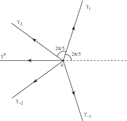
  Figure 2: The contour $\Gamma_{\Psi}$ associated with the Painlevé I equation

• Let $\Psi_{\pm}(\zeta;s)$ denote the limiting values of $\Psi(\zeta;s)$ as $\zeta$ tends to the contour $\Gamma_{\Psi}$ from the left and right sides, respectively. Then, $\Psi(\zeta;s)$ satisfies the following jump conditions

  $$\Psi_{+}(\zeta;s)=\Psi_{-}(\zeta;s)\left\{\begin{array}[]{ll}\left(\begin{array}[]{cc}1&s_{i}\\ 0&1\\ \end{array}\right),&z\in\gamma_{k},\ k=\pm 1;\\[11.38092pt] \left(\begin{array}[]{cc}1&0\\ i&1\\ \end{array}\right),&z\in\gamma_{k},\ k=\pm 2;\\[11.38092pt] \left(\begin{array}[]{cc}0&-i\\ -i&0\\ \end{array}\right),&z\in\gamma^{*},\end{array}\right.$$ (1.21)

  where $s_{1}=(1-\alpha)i$ and $s_{-1}=\alpha i$, with $\alpha$ being a complex constant.

• As $\zeta\to\infty$, $\Psi(\zeta;s)$ satisfies the asymptotic condition

  $$\Psi(\zeta;s)=\zeta^{\frac{1}{4}\sigma_{3}}\frac{\sigma_{3}+\sigma_{1}}{\sqrt{2}}\left(I+\frac{\Psi_{-1}(s)}{\sqrt{\zeta}}+\frac{\Psi_{-2}(s)}{\zeta}+O(\zeta^{-\frac{3}{2}})\right)e^{\theta(\zeta,s)\sigma_{3}}$$ (1.22)

  for $\arg\zeta\in(-\pi,\pi)$, where

  $$\theta(\zeta,s)=\frac{4}{5}\zeta^{\frac{5}{2}}+s\zeta^{\frac{1}{2}},$$ (1.23)

  $\sigma_{1}$ and $\sigma_{3}$ are the Pauli matrices

  $$\sigma_{1}=\begin{pmatrix}0&1\\ 1&0\end{pmatrix},\qquad\sigma_{3}=\begin{pmatrix}1&0\\ 0&-1\end{pmatrix}.$$

It is known that, for each $\alpha\in\mathbb{C}$,

$$y_{\alpha}(s)=2(\Psi_{-2}(s))_{12}$$ (1.24)

is a solution of the Painlevé I equation (1.19). As a consequence, the above RH problem for $\Psi(\zeta;s)$ has a solution if and only if $s$ is not a pole of $y_{\alpha}(s)$. Due to the meromorphic property of the Painlevé I transcendents, one also see that the solution of the above RH problem for $\Psi(\zeta;s)$ is meromorphic in the parameter $s$. Moreover, it is shown in Kapaev [21] that $y_{\alpha}(s)$ is the so-called tronquée solution of Painlevé I whose asymptotic behavior is given by

$$y_{\alpha}(z)=y_{0}(z)+\frac{\alpha i}{\sqrt{\pi}}2^{-\frac{11}{8}}(-3z)^{-\frac{1}{8}}\exp\left[-\frac{1}{5}2^{\frac{11}{4}}3^{\frac{1}{4}}(-z)^{\frac{5}{4}}\right]\left(1+O(z^{-\frac{3}{8}})\right)$$ (1.25)

as $z\to\infty$ and $\arg z=\arg(-z)+\pi\in[\frac{3}{5}\pi,\pi]$. Here $y_{0}(z)$ is the tritronquée solution satisfying

$$y_{0}(z)\sim\sqrt{-z/6}\left[1+\sum_{k=1}^{\infty}a_{k}(-z)^{-5k/2}\right]\quad\textrm{as }z\to\infty,\ -\frac{\pi}{5}<\arg z<\frac{7\pi}{5},$$ (1.26)

where the coefficients $a_{k}$ can be determined recursively; see for example Joshi and Kitaev [20]. The solution $y_{\alpha}(z)$ will appear in our main results below.

We mention several known facts about the coefficients in (1.22) in addition to (1.24). For example, the explicit formulas of $\Psi_{-1}(s)$ and $\Psi_{-2}(s)$ are given in [21] as

$$\Psi_{-1}(s)=-\mathcal{H}_{\alpha}(s)\sigma_{3},\qquad\Psi_{-2}(s)=\frac{1}{2}\biggl{(}\mathcal{H}_{\alpha}^{2}(s)I+y_{\alpha}(s)\sigma_{1}\biggr{)},$$ (1.27)

where

$$\mathcal{H}_{\alpha}(s)=\frac{1}{2}y_{\alpha}^{\prime 2}(s)-2y_{\alpha}^{3}(s)-sy_{\alpha}(s)$$ (1.28)

is the Hamiltonian of Painlevé I.

1.2 Statement of main results

First of all, when the degree $k$ is fixed, we show that the recurrence coefficient $\alpha_{k,n}(t)$ satisfies a particular Painlevé III equation with certain initial conditions. Moreover, we prove that the Hankel determinant $D_{k}[w(z;t)]$ is related to the $\tau$-function of the Painlevé III equation. Similar results for the weight in (1.17) have been obtained by Chen and Its [9].

Theorem 1.

For fixed non-negative integer $k$, let $\alpha_{k,n}$ be the recurrence coefficient in (1.5), and

$$a_{k,n}(t)=\alpha_{k,n}(t)-\frac{2k+1+n}{n}.$$ (1.29)

Then $a_{k}(t)=a_{k,n}(t)$ satisfies the following Painlevé III equation

$$a_{k}^{\prime\prime}=\frac{(a_{k}^{\prime})^{2}}{a_{k}}-\frac{a_{k}^{\prime}}{t}+n(2k+1+n)\frac{a_{k}^{2}}{t^{2}}+\frac{n^{2}a_{k}^{3}}{t^{2}}+\frac{n^{2}}{t}-\frac{n^{2}}{a_{k}},$$ (1.30)

with the initial conditions $a_{k}(0)=0$, $a_{k}^{\prime}(0)=1$. Moreover, we have

$$D_{k}[w;t]=\mathrm{const}\cdot\tau(t)\;e^{{n^{2}t}/{2}}\;t^{{k(k+n)}/{2}},$$ (1.31)

where $\tau(t)$ is the Jimbo-Miwa-Ueno isomonodromy $\tau$-function of the above Painlevé III equation.

Next, we let $k=n$ and consider the double scaling limit when $n\to\infty$ and $t\to t_{cr}$ simultaneously. We show that the asymptotics of the Hankel determinant $D_{n}[w(z;t)]$ associated with the weight in (1.8) can be expressed in terms of the tronquée solution $y_{\alpha}(s)$ of Painlevé I equation given in (1.24).

Theorem 2.

Let the constants $t_{cr}$, $a_{cr}$ and $b_{cr}$ be defined as

$$t_{cr}=-\frac{3}{4}(2^{1/3}-1)^{2}\approx-0.051$$ (1.32)

and

$$a_{cr}=\frac{1}{2}(3-2^{1/3}-2^{2/3})\approx 0.076,\quad b_{cr}=\frac{3}{2}(1+2^{1/3}+2^{2/3})\approx 5.771.$$ (1.33)

For $n\to\infty$ and $t\to t_{cr}$ in a way such that

$$s^{*}=\left\{(2a_{cr})^{-\frac{3}{5}}(a_{cr}b_{cr})^{-\frac{1}{2}}(b_{cr}-a_{cr})^{\frac{2}{5}}\right\}n^{\frac{4}{5}}(t_{cr}-t)$$ (1.34)

remains bounded. Suppose $\alpha\in\mathbb{C}$ is fixed and $s^{*}$ is not a pole of the tronquée solution $y_{\alpha}(s)$, then an asymptotic approximation of the logarithmic derivative of the Hankel determinant $H_{n,n}=t\frac{d}{dt}\log D_{n}[w;t]$ associated with the weight function (1.6) is given by

$$\frac{d}{dt}H_{n,n}(t)=-\frac{n^{2}}{4}\left(\sqrt{\frac{a_{cr}}{b_{cr}}}+\sqrt{\frac{b_{cr}}{a_{cr}}}-2-\frac{1}{n^{\frac{2}{5}}}\frac{2(b_{cr}-a_{cr})^{\frac{4}{5}}}{(2a_{cr})^{\frac{1}{5}}\sqrt{a_{cr}b_{cr}}}y_{\alpha}(s^{*})+O\left(\frac{1}{n^{\frac{3}{5}}}\right)\right).$$ (1.35)

We would also derive the double scaling limit of the recurrence coefficients and the leading coefficients of the orthonormal polynomials.

Theorem 3.

Under the same conditions as in the previous theorem, the monic polynomial $\pi_{n,n}(z)$ defined in (1.8) exists for large enough $n$ and $t$ close to $t_{cr}$. Moreover, we have the asymptotics of the recurrence coefficients

$$a_{n,n}=\frac{t}{\sqrt{a_{cr}b_{cr}}}\left(1-\frac{2^{4/5}y_{\alpha}(s^{*})}{a_{cr}^{1/5}(b_{cr}-a_{cr})^{1/5}n^{2/5}}+O\left(\frac{1}{n^{3/5}}\right)\right),$$ (1.36)

$$\beta_{n,n}=\frac{(b_{cr}-a_{cr})^{2}}{16}-\frac{(2a_{cr}(b_{cr}-a_{cr}))^{4/5}y_{\alpha}(s^{*})}{4}\frac{1}{n^{2/5}}+O\left(\frac{1}{n^{3/5}}\right)$$ (1.37)

and

$$\gamma_{n,n}^{2}=\frac{2}{\pi(b_{cr}-a_{cr})}e^{-nl}\left(1+\frac{2(2a_{cr})^{4/5}\mathcal{H}_{\alpha}(s^{*})}{(b_{cr}-a_{cr})^{1/5}n^{1/5}}+O\left(\frac{1}{n^{2/5}}\right)\right),$$ (1.38)

where $\mathcal{H}_{\alpha}(s)$ is the Hamiltonian of Painlevé I given in (1.28).

Remark 1.

It is well-known that the tronquée solutions of Painlevé I are meromorphic functions and possess infinitely many poles in the complex plane. Therefore, to make the results valid in the above theorems, we require the $s^{*}$ in (1.34) is bounded away from the poles of $y_{\alpha}(s)$. Recently, through a more delicate triple scaling limit, Bertola and Tovbis [4] successfully obtain the asymptotics near the poles of $y_{\alpha}(s)$. Similar results near the poles of $y_{\alpha}(s)$ might be derived by using their ideas in [4]. However, we do not pursue that part. Instead, we focus on the main task of the present paper to demonstrate that the Painlevé I asymptotics can also occur for the weight (1.1) with negative $t$.

The rest of the paper is arranged as follows. In Section 2, we provide a RH problem for the orthogonal polynomials with respect to the weight (1.6). A transformed version of the solution is shown to fulfill a Lax pair, which is closely related to the Painlevé III equation. Several differential identities are stated and justified. Theorem 1 is also proved in this section. Section 3 is devoted to the determination of equilibrium measures, involving a positive measure and a signed measure. In Section 4, we carry out a nonlinear steepest descent analysis of the RH problem for the orthogonal polynomials. Particular attention will be paid to the construction of the local parametrix at the critical endpoint $z=a_{cr}$, where the Painlevé I transcendents are involved. Then, the proofs of Theorems 2 and 3 are given in the last section, Section 5.

2 Finite Hankel determinants and Painlevé III equation

In this section, we state the RH problem for the perturbed Laguerre orthogonal polynomials. Then we show that after some elementary transformations, the RH problem is transformed into a RH problem for the Painlevé III equation. As a consequence, we derive a Painlevé III equation satisfied by the recurrence coefficient $\alpha_{k,n}$ up to a translation, and establish a relation between the finite Hankel determinant of the perturbed Laguerre weight in (1.8) with the $\tau$-function of this Painlevé III equation. Several differential identities for the Hankel determinants and the recurrence coefficients of the perturbed Laguerre orthogonal polynomials are also derived. The identities are important in the asymptotic analysis in later sections. Although our calculations are similar to those in Chen and Its [9], we think it is convenient for the reader to have more details.

2.1 Riemann-Hilbert problem for orthogonal polynomials and differential identities

We state the RH problem for the perturbed Laguerre orthogonal polynomials as follows:

• $Y(z)$ is analytic in $\mathbb{C}\backslash\Gamma_{j}$, $j=1,2,3$; see Figure 1;

• $Y(z)$ satisfies the jump condition

  $$Y_{+}(z)=Y_{-}(z)\left(\begin{array}[]{cc}1&w(z;t)\\ 0&1\\ \end{array}\right),\qquad z\in\Gamma=\Gamma_{1}\cup\Gamma_{2}\cup\Gamma_{3},$$ (2.1)

  where $w(z;t)$ is the weight function piecewise-defined in (1.6);

• The asymptotic behavior of $Y(z)$ at infinity is

  $$Y(z)=\left(I+O\left(1/z\right)\right)\left(\begin{array}[]{cc}z^{k}&0\\ 0&z^{-k}\\ \end{array}\right),\quad\mbox{as}\quad z\rightarrow\infty;$$ (2.2)

• As $z\to 0$, $Y(z)=O(1)$.

Using a by now standard argument, originally due to Fokas, Its, and Kitaev [17], the solution of the above RH problem, if it exists, is uniquely given by

$$Y(z)=\left(\begin{array}[]{cc}\pi_{k}(z)&\frac{1}{2\pi i}\int_{\Gamma}\frac{\pi_{k}(s)w(s;t)}{s-z}ds\\[5.69046pt] -2\pi i\gamma_{k-1}^{2}\;\pi_{k-1}(z)&-\gamma_{k-1}^{2}\;\int_{\Gamma}\frac{\pi_{k-1}(s)w(s;t)}{s-z}ds\end{array}\right),$$ (2.3)

where $\pi_{k}(z)=\pi_{k,n}(z)$ is the monic perturbed Laguerre orthogonal polynomials defined in (1.8) and $\gamma_{k}=\gamma_{k,n}(t)$ is the leading coefficient for the orthonormal polynomial of degree $k$. To show the existence of $\pi_{n,n}(z)$ when $n$ is large enough, we will apply a series of invertible transformations to transform the original RH problem $Y$ to a new RH problem for $R$, which is solvable for sufficiently large $n$, $t$ close to $t_{cr}$ as in (1.34), and $s^{*}$ is not a pole of the tronquée solution $y_{\alpha}(s)$. Tracing back the invertible transformations, we will see that the RH problem is solvable under the same conditions. Indeed, it is also possible to prove the solvability for $t\geq t_{cr}$. However, since we are interested in the phase transition near $t_{cr}$, we don’t consider the case when $t_{cr}<t<0$ in the subsequent analysis. Thus, the perturbed Laguerre orthogonal polynomials are well-defined for $k=n$ large enough.

Next, we derive some differential identities for the recurrence coefficients and the logarithmic derivative of the Hankel determinant associated with the perturbed Laguerre weight $w(z)=w(z;t)$ in (1.6). The results are expressed in terms of the entries of $Y(z)$.

Lemma 1.

Assume that $t>0$. Let $\alpha_{k,n}(t)$ and $\beta_{k,n}(t)$ be the recurrence coefficients in (1.5), and $D_{k}[w;t]$ be the Hankel determinant in (1.3). Define

$$a_{k,n}(t)=\alpha_{k,n}(t)-\frac{1}{n}(2k+1+n)$$ (2.4)

and

$$H_{k,n}(t)=t\frac{d}{dt}\log D_{k}[w;t].$$ (2.5)

Then we have

$$a_{k,n}(t)=t\gamma_{k,n}^{2}\int_{\Gamma}\frac{\pi_{k,n}^{2}(z)w(z;t)}{z}dz=2\pi it\gamma_{k,n}^{2}(t)Y_{11}(0)Y_{12}(0),$$ (2.6)

$$\beta_{k,n}(t)=\frac{1}{n^{2}}\biggl{[}k(k+n)+t\frac{d}{dt}H_{k,n}(t)-H_{k,n}(t)\biggr{]}$$ (2.7)

and

$$\frac{d}{dt}H_{k,n}(t)=n^{2}\gamma_{k-1,n}^{2}\int_{\Gamma}\frac{\pi_{k-1,n}(z)\pi_{k,n}(z)w(z;t)}{z}dz=-n^{2}Y_{12}(0)Y_{21}(0).$$ (2.8)

Proof.

Since $t>0$, the orthogonal polynomials $\pi_{k,n}$ exist for all nonnegative $k$ and positive $n$. First, we consider the recurrence coefficient $\alpha_{k,n}(t)$. Based on the three-term recurrence relation (1.5) and the orthogonality condition (1.8), we get

$$\alpha_{k,n}(t)=\gamma_{k,n}^{2}(t)\int_{\Gamma}z\pi_{k,n}^{2}(z)w(z)dz.$$ (2.9)

Using the fact that $w(z)=\frac{w(z)}{z}+\frac{tw(z)}{z^{2}}-\frac{w^{\prime}(z)}{n}$ and integrating by part once, the above formula gives us

$$a_{k,n}(t)=t\gamma_{k,n}^{2}(t)\int_{\Gamma}\frac{\pi_{k,n}^{2}(z)w(z)}{z}dz.$$ (2.10)

Then (2.6) follows from a partial fraction decomposition of $\frac{\pi_{k,n}(z)}{z}$, the orthogonality condition (1.8), and the explicit expression of $Y(z)$ in (2.3).

Next, we consider the Hankel determinant. Recall that the Hankel determinant can be expressed in terms of the leading coefficients as

$$D_{k}[w;t]=\prod_{j=0}^{k-1}\gamma_{j,n}^{-2}(t);$$

see (1.4). Taking logarithmic derivative of both sides of the above equation with respect to $t$ and using the integral representation of the leading coefficients in (1.8), we get

$$H_{k,n}(t)=-n\sum_{j=0}^{k-1}a_{j,n}(t).$$ (2.11)

Differentiating the above formula again, we get from (2.4)

$$\frac{d}{dt}H_{k,n}(t)=-n\frac{d}{dt}\sum_{j=0}^{k-1}\alpha_{j,n}(t).$$ (2.12)

Let $\mathfrak{p}_{k,n}(t)$ be the coefficient of the $z^{k-1}$ term in $\pi_{k,n}(z)$, i.e.,

$$\pi_{k,n}(z)=z^{k}+\mathfrak{p}_{k,n}(t)z^{k-1}+\cdots.$$ (2.13)

Comparing the $x^{k}$ powers in the recurrence relation (1.5), we obtain

$$\alpha_{k,n}=\mathfrak{p}_{k,n}(t)-\mathfrak{p}_{k+1,n}(t).$$ (2.14)

To derive $\frac{d}{dt}H_{k,n}(t)$, one can see from (2.12) and (2.14) that it is sufficient to obtain $\frac{d}{dt}\mathfrak{p}_{k,n}(t)$. This can be done by taking derivative of the following orthogonal formula with respect to the parameter $t$

$$\int_{\Gamma}\pi_{k,n}(z)\pi_{k-1,n}(z)w(z)dz=0.$$

More precisely, taking into account the orthogonal relation (1.8) and the fact that $\frac{\partial w(z;t)}{\partial t}=-\frac{n}{z}w(z;t)$, we have

$$\frac{d}{dt}\mathfrak{p}_{k,n}(t)=n\gamma_{k-1,n}^{2}\int_{\Gamma}\frac{\pi_{k,n}(z)\pi_{k-1,n}(z)w(z)}{z}dz.$$ (2.15)

Then, (2.8) follows from a combination of (2.12), (2.14) and (2.15), as well as the definition of $Y(z)$ in (2.3).

Finally, let us study $\beta_{k,n}(t)$. Using the ideas leading to (2.10), we have

$$\beta_{k,n}(t)=t\gamma_{k-1,n}^{2}\int_{\Gamma}\frac{\pi_{k,n}(z)\pi_{k-1,n}(z)w(z)}{z}dz-\frac{1}{n}\mathfrak{p}_{k,n}(t),$$ (2.16)

where $\mathfrak{p}_{k,n}(t)$ is introduced in (2.13). The first term on the right-hand side is $\frac{t}{n^{2}}\frac{d}{dt}H_{k,n}(t)$; cf. (2.8). An expression for the term on the extreme right can be obtained by deriving $\mathfrak{p}_{k,n}(t)=\sum_{j=0}^{k-1}\alpha_{j,n}$ from (2.14), and using (2.4) and (2.11).

This completes the proof of our lemma. ∎

Remark 2.

For later use, we need the differential identities of Lemma 1 in the case when $k=n$ is large and $t\sim t_{cr}$. They can be obtained through an analytic continuation argument. Indeed, $Y(z)$ determined by RH problem exists in this case, and is related to the $\Psi$-function of the third Painlevé equation after an elementary transformation given in (2.17). Thus $Y(z)$ is meromorphic with respect to $t$ in the cut plane $\arg(-t)\in(-\pi/2,3\pi/2)$. In particular, both $Y$ and the Hankel determinant are analytic in a domain containing the interval $t>0$ and a neighborhood of $t=t_{cr}$. Note that the identities (2.6)-(2.8) hold for $t>0$, then, by analytic continuation, they also hold for $t$ close to $t_{cr}$. We conclude that for $k=n$ large and $t\sim t_{cr}$, the identities (2.6)-(2.8) are also true. Similar argument has previously been used in Bleher and Deaño [5].

2.2 Relation to the Painlevé III equation

Introduce a purely imaginary parameter $s=ni\sqrt{-t}$, and define

$$\Phi(\lambda,s)=\left(\frac{ni}{s}\right)^{(\frac{n}{2}+k)\sigma_{3}}Y\left(\frac{s\lambda}{ni}\right)e^{\frac{i}{2}(s\lambda-\frac{s}{\lambda})\sigma_{3}}\left(\frac{s\lambda}{ni}\right)^{\frac{n}{2}\sigma_{3}},~{}~{}\lambda\not\in\Gamma^{*},$$ (2.17)

where $\Gamma^{*}=\Gamma^{*}_{1}\cup\Gamma^{*}_{2}\cup\Gamma^{*}_{3}=\frac{1}{\sqrt{-t}}\Gamma$ is the rescaled contour. Then, $\Phi(\lambda)=\Phi(\lambda,s)$ solves the following RH problem with constant jumps:

• $\Phi(\lambda)$ is analytic for $\lambda\in\mathbb{C}\setminus\cup_{j=1}^{3}\Gamma^{*}_{j}$. As $\Gamma^{*}$ and $\Gamma$ only differ by a scale, one may refer to Figure 1 to see the properties of the contour $\Gamma^{*}$.

• $\Phi(\lambda)$ satisfies the jump condition

  $$\Phi_{+}(\lambda)=\Phi_{-}(\lambda)\left(\begin{array}[]{cc}1&c_{j}\\ 0&1\\ \end{array}\right),\quad\lambda\in\Gamma^{*}_{j},~{}j=1,2,3,$$ (2.18)

  where $c_{1}=1,c_{2}=\alpha,c_{3}=1-\alpha$; cf. (1.6).

• The asymptotic behavior of $\Phi(\lambda)$ at infinity is

  $$\Phi(\lambda)=\left(I+\sum_{k=1}^{\infty}\frac{\Phi_{-k}}{\lambda^{k}}\right)\lambda^{(\frac{n}{2}+k)\sigma_{3}}e^{\frac{is\lambda}{2}\sigma_{3}}\quad\mbox{as}\quad\lambda\rightarrow\infty,$$ (2.19)

  where

  $$\Phi_{-1}=\frac{ni}{s}\left(\frac{ni}{s}\right)^{(\frac{n}{2}+k)\sigma_{3}}\left(\begin{array}[]{cc}\mathfrak{p}_{k,n}(t)-\frac{s^{2}}{2n}&-\frac{1}{2\pi i\gamma_{k,n}(t)^{2}}\\ -2\pi i\gamma_{k-1,n}(t)^{2}&-\mathfrak{p}_{k,n}(t)+\frac{s^{2}}{2n}\\ \end{array}\right)\left(\frac{ni}{s}\right)^{-(\frac{n}{2}+k)\sigma_{3}},$$ (2.20)

  In the above formula, $\gamma_{k,n}$ and $\mathfrak{p}_{k,n}$ are, respectively, the leading coefficient of the $k$-th orthonormal polynomial, and the coefficient of the $z^{k-1}$ term in the $k$-th monic orthogonal polynomial introduced in (2.13), with respect to the varying perturbed Laguerre weight in (1.6) and (1.8).

• The asymptotic behavior of $\Phi(\lambda)$ at $\lambda=0$ is

  $$\Phi(\lambda)=\Phi(0)\left(I+\sum_{k=1}^{\infty}\Phi_{k}\lambda^{k}\right)\lambda^{\frac{1}{2}n\sigma_{3}}e^{-\frac{si}{2\lambda}\sigma_{3}}\quad\mbox{as}\quad\lambda\rightarrow 0,$$ (2.21)

  where

  $$\Phi(0)=\left(\frac{ni}{s}\right)^{(\frac{n}{2}+k)\sigma_{3}}\left(\begin{array}[]{cc}1&c_{k,n}(t)\\ -q_{k,n}(t)&1-c_{k,n}(t)q_{k,n}(t)\\ \end{array}\right)\pi_{k}(0)^{\sigma_{3}}\left(\frac{ni}{s}\right)^{-\frac{1}{2}n\sigma_{3}},$$ (2.22)

  with

  $$c_{k,n}(t)=\frac{\pi_{k}(0)}{2\pi i}\int_{\Gamma}\frac{\pi_{k}(z)w(z;t)}{z}dz~{}~{}\mbox{and}~{}~{}q_{k,n}(t)=2\pi i\gamma^{2}_{k-1,n}(t)\frac{\pi_{k-1}(0)}{\pi_{k}{(0)}}.$$

Now, from the above RH problem, we derive the following Lax pair for the function $\Phi(\lambda,s)$, which is exactly the same as the Lax pair for Painlevé III; see [18, pp.195-203].

Proposition 1.

For the matrix function $\Phi(\lambda,s)$ given in (2.17), we have

$$\Phi_{\lambda}=A(\lambda,s)\Phi\quad\textrm{and}\quad\Phi_{s}=B(\lambda,s)\Phi,$$ (2.23)

where

$$A(\lambda,s)=\frac{is}{2}\sigma_{3}+\frac{A_{-1}}{\lambda}+\frac{A_{-2}}{\lambda^{2}}\quad\textrm{and}\quad B(\lambda,s)=\frac{i\lambda}{2}\sigma_{3}+B_{0}+\frac{B_{-1}}{\lambda}.$$ (2.24)

Here, the coefficients in the above formula are given below

$$A_{-1}=\left(\begin{array}[]{cc}\frac{n}{2}+k&-\frac{n}{2\pi i\gamma_{k,n}^{2}}\left(\frac{ni}{s}\right)^{n+2k}\\ 2n\pi i\gamma_{k-1,n}^{2}\left(\frac{ni}{s}\right)^{-n-2k}&-\frac{n}{2}-k\\ \end{array}\right)$$ (2.25)

$$A_{-2}=\frac{is}{2}\left(\begin{array}[]{cc}1-2c_{k,n}q_{k,n}&-2c_{k,n}\left(\frac{ni}{s}\right)^{n+2k}\\ -2q_{k,n}(1-c_{k,n}q_{k,n})\left(\frac{ni}{s}\right)^{-n-2k}&2c_{k,n}q_{k,n}-1\\ \end{array}\right)$$ (2.26)

and

$$B_{0}=\frac{1}{s}\biggl{(}A_{-1}-\left(\frac{n}{2}+k\right)\sigma_{3}\biggr{)},\quad B_{-1}=-\frac{A_{-2}}{s}.$$ (2.27)

Proof.

Note that the jump matrices in (2.18) are independent of $\lambda$ and $s$. This implies that both

$$A(\lambda,s)=\Phi_{\lambda}\Phi^{-1}\quad\textrm{and}\quad B(\lambda,s)=\Phi_{s}\Phi^{-1}$$ (2.28)

are analytic functions of $\lambda$ with only possible isolated singularities at the origin and at infinity. Using the asymptotic expansions in (2.19)-(2.22), we find that

$$A_{-1}=\left(\frac{n}{2}+k\right)\sigma_{3}+\frac{is}{2}[\Phi_{-1},\sigma_{3}],\qquad A_{-2}=\frac{is}{2}\Phi(0)\sigma_{3}\Phi(0)^{-1}$$ (2.29)

and

$$B_{0}=\frac{i}{2}[\Phi_{-1},\sigma_{3}],\qquad B_{-1}=-\frac{A_{-2}}{s},$$ (2.30)

where $[X,Y]=XY-YX$ is the commutator. Then direct computations give us the results. ∎

It is known in several circumstances that the Hankel determinants admit an interpretation as the Jimbo-Miwa-Ueno isomonodromic $\tau$-function for the rank 2 linear system of differential equations; see [16] for the Hankel determinants associated with the exponential weight and [2, 3] for more general semi-classical weights. Now we have established the relation between the perturbed Laguerre orthogonal polynomials and the Lax pair for the Painlevé III equation. Naturally, the associated Hankel determinant is also expected to relate to the $\tau$-function of the Painlevé III equation. Thus we are in a position to prove our first result for fixed degree $k$.

Proof of Theorem 1. According to Proposition 1, $\Phi(\lambda,s)$ satisfies the same Lax pair as Painlevé III. Then, applying an argument in [18, (5.3.4),(5.3.7)], we see that the function

$$u(s)=-i(A_{-1})_{12}/{(A_{-2})_{12}}=-\frac{n}{2\pi isc_{k,n}\gamma_{k,n}^{2}}$$ (2.31)

solves the Painlevé III equation

$$u^{\prime\prime}(s)=\frac{(u^{\prime})^{2}}{u}-\frac{u^{\prime}}{s}+\frac{4}{s}(\Theta_{0}u^{2}+1-\Theta_{\infty})+4u^{3}-\frac{4}{u},$$ (2.32)

with the parameters $\Theta_{0}=n$ and $\Theta_{\infty}=-(2k+n)$. By (2.6), we have

$$u(s)=-\frac{nt}{sa_{k,n}}=\frac{\sqrt{-t}}{ia_{k,n}}.$$ (2.33)

Substituting (2.33) into (2.32) gives us (1.30).

Next, we consider the Hankel determinant $D_{k}[w;t]$. Denote by $\Phi_{\infty}(\lambda)$ and $\Phi_{0}(\lambda)$ the series in the expansions (2.19) and (2.21), namely,

$$\Phi_{\infty}(\lambda)=I+\sum_{k=1}^{\infty}\frac{\Phi_{-k}}{\lambda^{k}}\quad\textrm{and}\quad\Phi_{0}(\lambda)=I+\sum_{k=1}^{\infty}\Phi_{k}\lambda^{k},$$

with $\Phi_{-1}$ qiven in (2.20) and

$$\Phi_{1}=\frac{1}{is}\left(-n^{2}\beta_{k,n}(t)-(k^{2}+nk)+\frac{s^{2}}{2}(1-2c_{k,n}(t)q_{k,n}(t))\right)\sigma_{3}+\left(\begin{array}[]{cc}0&*\\ &0\\ \end{array}\right);$$ (2.34)

cf. (2.3) and (2.17), where $*$ denotes the off-diagonal entries independent of $\lambda$. By the general theory of Jimbo-Miwa-Ueno [19], the isomonodromy $\tau$-function for the Lax pair in (2.23)-(2.27) is defined by the formula

$$d\log\tau(s):=-\operatorname*{{Res}}_{\lambda=0}\mathrm{Tr}\left\{\Phi_{0}^{-1}(\lambda)\frac{\partial\Phi_{0}(\lambda)}{\partial\lambda}dT_{0}(\lambda)\right\}-\operatorname*{{Res}}_{\lambda=\infty}\mathrm{Tr}\left\{\Phi_{\infty}^{-1}(\lambda)\frac{\partial\Phi_{\infty}(\lambda)}{\partial\lambda}dT_{\infty}(\lambda)\right\},$$ (2.35)

where

$$dT_{0}(\lambda)=-\frac{i}{2\lambda}\sigma_{3}ds,\quad dT_{\infty}(\lambda)=\frac{i\lambda}{2}\sigma_{3}ds;$$

see [19, Eq.(1.23)]. Substituting the definition of $\Phi_{\infty}(\lambda)$ and $\Phi_{0}(\lambda)$ into (2.35), we obtain

$$\frac{d\log\tau(s)}{ds}=\frac{i}{2}\mathrm{Tr}(\Phi_{1}\sigma_{3}-\Phi_{-1}\sigma_{3})=\frac{1}{s}\left(-2n^{2}\beta_{k,n}+2s^{2}c_{k,n}q_{k,n}-s^{2}+(k^{2}+nk)\right).$$ (2.36)

Now a combination of (2.8), (2.11), (2.14) and (2.16) gives

$$n^{2}\beta_{k,n}=n^{2}tc_{k,n}q_{k,n}-H_{k,n}+k(k+n);$$ (2.37)

see (2.26) for the definition of $c_{k,n}(t)$ and $q_{k,n}(t)$. Thus, we obtain from (2.36) and (2.37) that

$$\frac{d\log\tau(s)}{dt}=\frac{1}{2t}\left(2H_{k,n}-s^{2}-(k^{2}+nk)\right).$$ (2.38)

Here use has been made of the relation $s^{2}=n^{2}t$. In view of the formula (2.5), and integrating both sides of (2.38), we arrive at the following relation between the Hankel determinant $D_{k}[w;t]$ and the $\tau$-function of the Painlevé III equation:

$$D_{k}[w;t]=\mathrm{const}\cdot\tau(s)e^{{n^{2}t}/{2}}t^{{k(k+n)}/{2}},$$

which is (1.31). This completes the proof of Theorem 1. ∎

3 Equilibrium measures

The equilibrium measure with the external field $V_{t}(x)$ in (1.2) is given recently in Texier and Majumdar [27]. To obtain a double scaling limit at the critical time, we need a modified equilibrium problem, which will involve a signed measure. This signed measure will be used to construct the important $g$-function and $\phi$-function in the Riemann-Hilbert analysis. The idea of considering a modified equilibrium problem has been successfully applied to study similar double scaling limits in several different problems, such as varying quartic potentials by Claeys and Kuijlaars [10] and Duits and Kuijlaars [14], and a cubic potential by Bleher and Deaño [6].

In this section, we will go back to the weight (1.1), consider a regular equilibrium problem first, and see how the critical time occurs. Then, to facilitate our future Riemann-Hilbert analysis near the critical time, we will consider a modified equilibrium problem by fixing the left endpoint. This will give us the signed measure we need.

3.1 Equilibrium measure and a critical case

Consider the extremal problem minimizing the energy with the external field $V_{t}(x)$ in (1.2):

$$I(\nu)=\int_{0}^{\infty}V_{t}(x)d\nu(x)+\int_{0}^{\infty}\int_{0}^{\infty}\log\frac{1}{|x-y|}d\nu(x)d\nu(y).$$ (3.1)

According to the general potential theory [24], there exists a unique minimizer $d\nu_{t}$ of $I(\nu)$ among all Borel probability measures $d\nu$ on $[0,+\infty)$, such a probability measure is called the equilibrium measure. For the potential $V_{t}(x)=x-\log x+t/x$ in (1.2), the equilibrium measure $d\nu_{t}$ can be computed explicitly.

The equilibrium measures for $t>t_{cr}$ and $t\to t_{cr}$ have been computed explicitly in Texier and Majumdar [27]. To make the present paper self-contained, we sketch the proof below, which differs from that in [27]. Inspired by [27], and in view of the measure for the positive-$t$ case, we assume that the support of $d\nu_{t}(x)$ has only one piece. Also, for fixed $t$, the behavior of the density $v_{t}(x)$ is expected to demonstrate a weak singularity at the endpoints since the contour is deformed to keep away from the possible singularity at the origin. We derive the equilibrium measure by solving a scalar RH problem, based on the Euler-Lagrange equation (3.4).

Proposition 2.

Let $v_{t}(x)$ be the density function of the equilibrium measure $d\nu_{t}$ supported on an interval $(a,b)\subset[0,\infty)$, such that $d\nu_{t}(x)=v_{t}(x)dx$. Then for $t>t_{cr}$ we have

$$v_{t}(x)=\frac{x+c}{2\pi x^{2}}\sqrt{(x-a)(b-x)},\qquad x\in(a,b),$$ (3.2)

where $c=t/\sqrt{ab}$ and $a,b$ are determined by (1.15). Moreover, when $t=t_{cr}$ as in (1.32), we have

$$v_{cr}(x)=\frac{1}{2\pi x^{2}}\sqrt{(x-a_{cr})^{3}(b_{cr}-x)},\qquad x\in(a_{cr},b_{cr}),$$ (3.3)

where the critical endpoints $a_{cr}$ and $b_{cr}$ are given in (1.33).

Proof.

From (3.1), it is known that the equilibrium measure $d\nu_{t}$ satisfies the Euler-Lagrange equation

$$V_{t}(x)+2\int_{a}^{b}\log\frac{1}{|x-y|}d\nu_{t}(y)=l,\qquad x\in(a,b),$$ (3.4)

where $l$ is the Lagrange multiplier. Differentiating with respect to $x$, we get

$$V^{\prime}_{t}(x)-2\,\textrm{p.v.}\int_{a}^{b}\frac{v_{t}(y)}{x-y}dy=0,\quad x\in(a,b).$$ (3.5)

where the integral is taken as the Cauchy principle value. This is an integral equation for the density function $v_{t}(x)$, which can be solved explicitly. Indeed, one can define

$$G(z)=\frac{1}{\pi i}\int_{a}^{b}\frac{v_{t}(y)}{y-z}dy,\quad z\in\mathbb{C}\setminus[a,b].$$ (3.6)

Then it follows from the Plemelj formula that

$$G_{\pm}(x)=\frac{1}{\pi i}\textrm{p.v.}\int_{a}^{b}\frac{v_{t}(y)}{y-x}dy\pm v_{t}(x),\quad x\in(a,b),$$ (3.7)

where the integral is the Cauchy principle value. It is readily verified that $G(z)$ satisfies the following scalar Riemann-Hilbert problem:

• $G(z)$ is analytic for $z\in\mathbb{C}\setminus[a,b]$ , having at most weak singularities at $z=a,\;b$;

• $G_{+}(x)+G_{-}(x)=-\frac{1}{\pi i}V^{\prime}_{t}(x)$ for $x\in(a,b)$;

• $G(z)\sim-\frac{1}{\pi iz}$ as $z\to\infty$.

Solving this RH problem yields

$$G(z)=-\frac{V_{t}^{\prime}(z)}{2\pi i}+\frac{\tilde{c}z+c}{2\pi iz^{2}}\sqrt{(z-a)(z-b)},$$ (3.8)

where $V_{t}^{\prime}(z)=1-\frac{1}{z}-\frac{t}{z^{2}}$, $c=\frac{t}{\sqrt{ab}}$ and $\tilde{c}=\frac{1}{\sqrt{ab}}\left[1+\frac{t}{2}\left(\frac{1}{a}+\frac{1}{b}\right)\right]$. Here attention should be paid to the fact that $G(z)$ is analytic outside the interval $[a,b]$, especially at $z=0$. Now expanding (3.8) in powers of $1/z$, the large-$z$ behavior of $G(z)$ ensures that

$$\tilde{c}=1~{}~{}\mbox{and}~{}~{}c-\frac{a+b}{2}=-3,$$

which are indeed (1.15). Furthermore, a combination of (3.7) and (3.8) yields (3.2).

Moreover, in the critical case when

$$c_{cr}=-a_{cr}$$

a straightforward computation gives us (1.32)-(1.33). ∎

Remark 3.

Of course, the formulas for the density function and endpoints in (3.2) and (1.15) hold when $t\geq 0$. For any $t\geq 0$, the density function is supported on $[a,b]$ with $0<a<b$ and vanishes like square roots at both endpoints. As a consequence, one will obtain usual Airy-type and sine-type asymptotic expansions for the orthogonal polynomials near the endpoints and inside the support, respectively.

3.2 Signed equilibrium measure

The critical case when $t=t_{cr}$ is termed a freezing transition; see [27]. One can see that, when $t=t_{cr}$, the density function $v_{t}(x)$ in (3.3) vanishes like a $3/2$ root at $a_{cr}$. This suggests that the local behavior of the orthogonal polynomials near $a_{cr}$ is described in terms of the Painlevé I transcendents; see [6, 14]. To precisely construct a local parametrix near the endpoint $a_{cr}$ by using the Painlevé I transcendents, a delicate study near $a_{cr}$ is needed in our subsequent nonlinear steepest descent analysis for the RH problem. Therefore, technically it is more convenient to have a measure whose left endpoint of the support is exactly located at $a_{cr}$. Note that in the case when only positive measures are involved as in Section 3.1, both endpoints $a$ and $b$ in (1.15) vary when the value of parameter $t$ changes. So we need to minimize the same energy functional (3.1) among signed measures on $[a_{cr},+\infty)$ which are nonnegative except possibly on $[a_{cr},a_{cr}+\delta_{1}]$ for some sufficiently small $\delta_{1}>0$. As there is no symmetry as in [14], the right endpoint $b$ may depend on $t$. A similar treatment is also employed in [6].

By a similar argument performed in Section 3.1, we find the new minimizer explicitly.

Proposition 3.

Let $\psi_{t}(x)$ be the signed density function of the minimizer of the minimizer of the energy functional in (3.1) on $[a_{cr},+\infty)$. Then we have

$$\psi_{t}(x)=\frac{1}{2\pi x^{2}}\sqrt{\frac{b-x}{x-a_{cr}}}\left(x^{2}+d_{1}x+d_{0}\right),~{}~{}x\in[a_{cr},b],$$ (3.9)

where

$$d_{0}=-t\sqrt{\frac{a_{cr}}{b}}\quad\textrm{and}\quad d_{1}=-\sqrt{\frac{a_{cr}}{b}}\left(1-\frac{t}{2a_{cr}}+\frac{t}{2b}\right)$$ (3.10)

and $b$ is determined by the equation

$$\sqrt{\frac{a_{cr}}{b}}\left(1-\frac{t}{2a_{cr}}+\frac{t}{2b}\right)+\frac{b-a_{cr}}{2}=3.$$ (3.11)

It is worth noting that for $t=t_{cr}$, the density of the modified equilibrium measure $\psi_{t}(x)$ is reduced to $v_{cr}(x)$ in (3.3). Moreover, near the critical time $t=t_{cr}$, we have

$$\begin{array}[]{ll}&b=b_{cr}+\sqrt{\frac{b_{cr}}{a_{cr}}}(b_{cr}-a_{cr})^{-1}(t-t_{cr})+O\left((t-t_{cr})^{2}\right),\\[5.69046pt] &d_{0}=a_{cr}^{2}-\sqrt{\frac{a_{cr}}{b_{cr}}}\frac{2b_{cr}-a_{cr}}{2(b_{cr}-a_{cr})}(t-t_{cr})+O\left((t-t_{cr})^{2}\right),\\[5.69046pt] &d_{1}=-2a_{cr}+\frac{1}{2}\sqrt{\frac{b_{cr}}{a_{cr}}}(b_{cr}-a_{cr})^{-1}(t-t_{cr})+O\left((t-t_{cr})^{2}\right).\end{array}$$ (3.12)

Based on the signed measure obtained above, we define several auxiliary functions which will be used in our further analysis.

Definition 1.

The $g$-function is defined as

$$g(z)=\int_{a_{cr}}^{b}\log(z-s)\psi_{t}(s)ds\quad\mbox{for}\quad z\in\mathbb{C}\setminus(-\infty,b],$$ (3.13)

where $\arg(z-s)\in(-\pi,\pi)$, and the equilibrium density function $\psi_{t}(x)$ is given in (3.9).

Definition 2.

We also define the following $\phi$-functions

$$\phi_{t}(z) = \frac{1}{2}\int_{a_{cr}}^{z}\frac{(s^{2}+d_{1}s+d_{0})(s-b)^{1/2}}{s^{2}(s-a_{cr})^{1/2}}ds,\ z\in\mathbb{C}\setminus\{(-\infty,0)\cup(a_{cr},\infty)\},$$ (3.14)

$$\phi_{cr}(z) = \frac{1}{2}\int_{a_{cr}}^{z}\frac{(s-a_{cr})^{3/2}(s-b_{cr})^{1/2}}{s^{2}}ds,\ z\in\mathbb{C}\setminus\{(-\infty,0)\cup(a_{cr},\infty)\},$$ (3.15)

where the branches are chosen such that $\arg(s-a_{cr})\in(0,2\pi)$, $\arg(s-b_{cr})\in(0,2\pi)$ and $\arg(s-b)\in(0,2\pi)$.

From the above definitions, it is immediately seen that $g(z)$ satisfies the Euler-Lagrange equation

$$g_{+}(x)+g_{-}(x)-V_{t}(x)-l=0,\quad x\in(a_{cr},b),$$ (3.16)

and the variational inequality

$$2g(x)-V_{t}(x)-l<0,~{}x\in(b,\infty),$$ (3.17)

where $l$ is the Lagrange multiplier introduced in (3.4). Moreover, the $g$-function and the $\phi$-function are related by

$$g_{+}(x)-g_{-}(x)=2\pi i-2\left(\phi_{t}\right)_{+}(x),\quad x\in(a_{cr},b).$$ (3.18)

Note that $\phi_{t}(z)$ and $\phi_{cr}(z)$ are close to each other when $t$ approaches $t_{cr}$. If we rewrite $\phi_{t}(z)$ as

$$\phi_{t}(z)=\phi_{cr}(z)+(t-t_{cr})\phi_{0}(z),$$ (3.19)

then, in view of (3.14)-(3.15), we have

$$\phi_{0}(z)=-i\frac{\sqrt{b_{cr}-a_{cr}}}{2a_{cr}\sqrt{a_{cr}b_{cr}}}\sqrt{z-a_{cr}}(1+r_{0}(z)),\quad\arg(z-a_{cr})\in(0,2\pi),$$ (3.20)

where $r_{0}(z)$ is analytic in a neighborhood of $z=a_{cr}$ and $r_{0}(a_{cr})=0$. We also need some local information of the functions $\phi_{cr}(z)$ and $\phi_{t}(z)$ at critical points $z=a_{cr}$ and $z=0$. From their definitions in (3.14) and (3.15), we have

$$\phi_{cr}(z)\sim\frac{(b_{cr}-a_{cr})^{\frac{1}{2}}}{5a_{cr}^{2}}(z-a_{cr})^{\frac{5}{2}}e^{\frac{1}{2}\pi i},\quad z\to a_{cr},$$ (3.21)

where $\arg(z-a_{cr})\in(0,2\pi)$, and

$$\phi_{t}(z)=\frac{t}{2z}-\frac{1}{2}\log z+O(1),\quad z\to 0,$$ (3.22)

where $\arg z\in(-\pi,\pi)$. From the above formula, one can see that $\operatorname{{Re}}\phi_{t}(z)>0$ if $t<0$ and $z$ approaches the origin such that $\cos(\arg z)<\frac{|z|\log|z|}{t}$; see Figures 3 and 4. In particular, we see that $e^{-n\phi_{t}(z)}$ is exponentially small as $z\to 0$, $z\in\Gamma_{2}$ or $z\in\Gamma_{3}$; cf. Figure 1 for the contours. In view of (3.19), one can see that the same holds for $e^{-n\phi_{cr}(z)}$. It is worth mentioning that on $\Gamma_{2}$ and $\Gamma_{3}$ with $|z-\delta|=\delta$, we have $\operatorname{{Re}}\frac{1}{z}\equiv\frac{1}{2\delta}$.

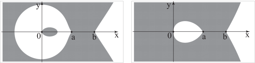
Figure 3: The shaded region is the region where $\operatorname{{Re}}\phi_{t}(z)<0$. The left and right pictures correspond to cases when $t<0$ and $t>0$, respectively.

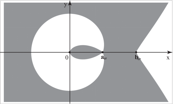
Figure 4: The shaded region is the region where $\operatorname{{Re}}\phi_{cr}(z)<0$. Note that this figure is not the exact one for $\phi_{cr}$ defined in (3.15). Here we have rescaled the figure, especially near $a_{cr}$, for better illustration: because the exact value of $a_{cr}$ is too small as compared with $b_{cr}$; see (1.33).

4 Nonlinear steepest descent analysis

In this section, we apply the nonlinear steepest descent method developed by Deift and Zhou et al. [12, 13] to the RH problem for $Y$. The idea is to obtain, via a series of invertible transformations $Y\to T\to S\to R$, the RH problem for $R$ whose jump matrices are close to the identity ones.

4.1 The first transformation $Y\to T$: Normalization at infinity

We make use of the $g$-function defined in (3.13) to normalize the RH problem for $Y$ in Section 2.1 when $k=n$. As $g(z)\sim\log z$ for large $z$, we introduce the first transformation $Y\to T$ as follows:

$$T(z)=e^{-\frac{nl}{2}\sigma_{3}}Y(z)e^{-n(g(z)-\frac{l}{2})\sigma_{3}},$$ (4.1)

where $l$ is the Lagrange multiplier in (3.16). Then, $T$ solves the following RH problem.

(T1)   $T(z)$ is analytic in $\mathbb{C}\backslash\Gamma$; see Figure 1 for $\Gamma=\Gamma_{1}\cup\Gamma_{2}\cup\Gamma_{3}$;

(T2)   The jump condition is

$$T_{+}(z)=T_{-}(z)\left(\begin{array}[]{cc}e^{n(g_{-}(z)-g_{+}(z))}&c_{j}e^{n(-V_{t}(z)+g_{+}(z)+g_{-}(z)-l)}\\ 0&e^{n(g_{+}(z)-g_{-}(z))}\\ \end{array}\right)$$ (4.2)

for $z\in\Gamma_{j}$, $j=1,2,3$, where $V_{t}(z)$ is defined in (1.7), and $c_{1}=1$, $c_{2}=\alpha$, $c_{3}=1-\alpha$;

(T3)   The asymptotic behavior of $T(z)$ at infinity is

$$T(z)=I+O(1/z)\quad\mbox{as}\quad z\rightarrow\infty.$$ (4.3)

Appealing to the properties of $g(z)$ and $\phi_{t}(z)$ in (3.16) and (3.18), the jump matrices in (4.2) can be expressed in terms of the function $\phi_{t}(z)$ as follows:

$$T_{+}(z)=T_{-}(z)\left\{\begin{array}[]{ll}\left(\begin{array}[]{cc}1&c_{j}e^{-2n\phi_{t}(z)}\\ 0&1\\ \end{array}\right),&z\in\Gamma_{j}\setminus(a_{cr},b),~{}j=1,2,3;\\[11.38092pt] \left(\begin{array}[]{cc}e^{2n\left(\phi_{t}\right)_{+}(z)}&1\\ 0&e^{2n\left(\phi_{t}\right)_{-}(z)}\\ \end{array}\right),&z\in(a_{cr},b).\end{array}\right.$$ (4.4)

4.2 The second transformation $T\to S$: Contour deformation

Since $\left(\phi_{t}\right)_{\pm}(z)$ are purely imaginary on $(a_{cr},b)$, the jump matrix for $T(z)$ on $z\in(a_{cr},b)$ possesses highly oscillatory diagonal entries. To remove the oscillation, we open the lens near $(a_{cr},b)$ and introduce the second transformation:

$$S(z)=\left\{\begin{array}[]{ll}T(z),&\mbox{for $z$ outside the lens shaped region;}\\[11.38092pt] T(z)\left(\begin{array}[]{cc}1&0\\ -e^{2n\phi_{t}(z)}&1\\ \end{array}\right),&\mbox{for $z$ in the upper lens region;}\\[11.38092pt] T(z)\left(\begin{array}[]{cc}1&0\\ e^{2n\phi_{t}(z)}&1\\ \end{array}\right),&\mbox{for $z$ in the lower lens region. }\end{array}\right.$$ (4.5)

Figure 5: Contour $\Sigma_{S}=(a_{cr},b)\cup(b,\infty)\cup_{j=2}^{5}\Gamma_{j}$. The shaded region is the region where $\operatorname{{Re}}\phi_{cr}(z)<0$.

Then $S(z)$ solves the RH problem

(S1)   $S(z)$ is analytic in $\mathbb{C}\setminus\Sigma_{S}$; see Figure 5 for the contours;

(S2)  The jump conditions are

$$S_{+}(z)=S_{-}(z)\left\{\begin{array}[]{ll}\left(\begin{array}[]{cc}1&0\\ e^{2n\phi_{t}(z)}&1\\ \end{array}\right),&z\in\Gamma_{4}\cup\Gamma_{5},\\[11.38092pt] \left(\begin{array}[]{cc}0&1\\ -1&0\\ \end{array}\right),&z\in(a_{cr},b),\\[11.38092pt] \left(\begin{array}[]{cc}1&\alpha e^{-2n\phi_{t}(z)}\\ 0&1\\ \end{array}\right),&z\in\Gamma_{2},\\[11.38092pt] \left(\begin{array}[]{cc}1&(1-\alpha)e^{-2n\phi_{t}(z)}\\ 0&1\\ \end{array}\right),&z\in\Gamma_{3},\\[11.38092pt] \left(\begin{array}[]{cc}1&e^{-2n\phi_{t}(z)}\\ 0&1\\ \end{array}\right),&z\in(b,+\infty).\end{array}\right.$$ (4.6)

(S3)   The asymptotic behavior at infinity is

$$S(z)=I+O(1/z),~{}~{}~{}\mbox{as}~{}~{}z\rightarrow\infty.$$ (4.7)

To study the asymptotic behavior of $S(z)$ for large $n$, we may exam the signs of $\operatorname{{Re}}\phi_{t}(z)$, to see if the jumps are of the form $I$ plus exponentially small terms. Special attention should be paid in the present case since we are dealing with the signed measure (3.9). Fortunately, when $n$ is large and $t-t_{cr}$ is small enough, we can still determine the signs of $\operatorname{{Re}}\phi_{t}(z)$ near the endpoint $a_{cr}$. Similar discussions can be found in [6, 14] where modified equilibrium problems are also addressed.

Proposition 4.

Let $U$ be a neighbourhood of $a_{cr}$. Then, for any $\varepsilon>0$, there exists a $\delta_{T}>0$ such that for all $t\in\mathbb{R}$ with $|t-t_{cr}|<{\delta_{T}}$, we have $\operatorname{{Re}}\phi_{t}(z)<-\varepsilon$ on the upper and lower lips of the lens on the outside of $U$, namely, $z\in\{\Gamma_{4}\cup\Gamma_{5}\}\setminus U$. Moreover, there exists a positive $r$, such that $\operatorname{{Re}}\phi_{t}(z)>\varepsilon$ on $\{\Gamma_{2}\cup\Gamma_{3}\}\setminus U$ and on $[b+r,\infty)$.

Proof.

In view of (3.12), we see that the factor $x^{2}+d_{1}x+d_{0}$ in (3.9) possesses a pair of zeros

$$x_{\pm}=a_{cr}\pm\frac{1}{\sqrt{2}}\left(\frac{a_{cr}}{b_{cr}}\right)^{1/4}(t-t_{cr})^{1/2}+O(t-t_{cr}).$$

One can choose $\delta_{T}$ small enough, so that $x_{\pm}\in U$. Similar to those conducted in [14, Prop. 4.2] and [6, p.23], we can prove that the jumps on the portions of $\Gamma_{4}$ and $\Gamma_{5}$, outside of $U$ and keeping a distance from the soft edge $b$, are of the form $I$ plus an exponentially small term.

Next, we estimate $\operatorname{{Re}}\phi_{t}(z)$ on $\Gamma_{2}\cup\Gamma_{3}\cup(b,\infty)$ in a straightforward manner, using the explicit representations of the $\phi$-functions (3.14), (3.15) and (3.19). In view of (3.19), we need only check the critical case for $\phi_{cr}$, and it is readily seen from (3.15) that

$$\operatorname{{Re}}\left(\phi_{cr}\right)_{\pm}(x)=\frac{1}{2}\int_{b_{cr}}^{x}\frac{(s-a_{cr})^{3/2}(s-b_{cr})^{1/2}}{s^{2}}ds>0~{}~{}\mbox{for}~{}x>b_{cr}.$$

For $z$ on the semi-circle $\Gamma_{2}$; cf. Figure 1, we take the integration path to be the arc from $a_{cr}$ to $z$, and adapt the parametrization $s=\delta+\delta e^{i\theta}$, where $\delta=a_{cr}/2$ and $\theta\in[0,\pi)$. As a result, we have

$$\phi_{cr}(z)=\frac{\sqrt{a_{cr}}}{4}\int_{0}^{\theta_{z}}\left\{|s-b_{cr}|^{\frac{1}{2}}\left(\sin\frac{\theta}{2}\right)^{\frac{3}{2}}\left(\cos\frac{\theta}{2}\right)^{-2}\right\}e^{i\left(\frac{5\pi}{4}+\frac{3\theta}{4}+\frac{1}{2}\arg(s-b_{cr})\right)}d\theta,$$ (4.8)

where $\theta_{z}\in[0,\pi)$ such that $z=\delta+\delta e^{i\theta_{z}}$. What is more, we have $\arg(s-b_{cr})\in[\pi-\arcsin A,\pi]\subset[3\pi/4,\pi]$ on $\Gamma_{2}$, where $A=\frac{a_{cr}}{2b_{cr}-a_{cr}}$ so that $\arcsin A\approx 0.0021\pi$. Hence the argument of the integrand lies in the interval $[2\pi-3\pi/8,2\pi+\pi/2)$, so long as $\theta\in[0,\pi)$. Therefore, from (4.8) we see that $\phi_{cr}(a_{cr})=0$, and $\operatorname{{Re}}\phi_{cr}(z)$ is strictly monotonically increasing as $z\in\Gamma_{2}$ goes away from $a_{cr}$. The same result holds for $z\in\Gamma_{3}$. It is worth mentioning that $\operatorname{{Re}}\phi_{t}(z)\to+\infty$ as $z\to 0$, $z\in\Gamma_{2}\cup\Gamma_{3}$; see the formula (3.22) and the discussion that follows. We note that the estimates on the lens boundaries $\Gamma_{4}$ and $\Gamma_{5}$ can also be obtained from the representations (3.14), (3.15) and (3.19). ∎

4.3 The global parametrix

Having had Proposition 4, we see from (4.6) that the jump matrix for $S$ is the identity matrix, plus an exponentially small term, for fixed $z$ bounded away from the interval $(a_{cr},b)$. Neglecting the exponentially small terms, we arrive at an approximating RH problem for $N(z)$ as follows:

(N1)   $N(z)$ is analytic in $\mathbb{C}\backslash[a_{cr},b]$;

(N2)

$$N_{+}(x)=N_{-}(x)\left(\begin{array}[]{cc}0&1\\ -1&0\\ \end{array}\right)~{}~{}~{}\mbox{for}~{}~{}x\in(a_{cr},b);$$ (4.9)

(N3)

$$N(z)=I+O(1/z)~{}~{}~{}\mbox{as}~{}~{}z\rightarrow\infty.$$ (4.10)

The solution to the above RH problem is constructed explicitly as

$$N(z)=M^{-1}\varrho(z)^{-\sigma_{3}}M,$$ (4.11)

where $M=(I+i\sigma_{1})/{\sqrt{2}}$ and $\varrho(z)=\left(\frac{z-b}{z-a_{cr}}\right)^{1/4}$ with $\arg(z-a_{cr})\in(-\pi,\pi)$ and $\arg(z-b)\in(-\pi,\pi)$.

The jump matrices of $S(z)N(z)^{-1}$ are not uniformly close to the identical matrix $I$ near the endpoints $a_{cr}$ and $b$, thus local parametrices have to be constructed in neighborhoods of these endpoints.

4.4 The local parametrix at the soft edge

The local parametrix at the right endpoint $z=b$ is the same as that of the Laguerre polynomials at the soft edge. More precisely, the parametrix is to be constructed in $U(b,r)=\{z~{}|\;|z-b|<r\}$, $r$ being a fixed positive number, such that

(a)   $P^{(b)}(z)$ is analytic in $U(b,r)\backslash\Sigma_{S}$; see Figure 5 for the contour $\Sigma_{S}$;

(b)   In $U(b,r)$, $P^{(b)}(z)$ satisfies the same jump conditions as $S(z)$ does; cf. (4.6);

(c)   $P^{(b)}(z)$ fulfils the following matching condition on $\partial U(b,r)$:

$$P^{(b)}(z)N^{-1}(z)=I+O\left(\frac{1}{n}\right).$$ (4.12)

The parametrix can be constructed, out of the Airy function and its derivative, as in [28, (3.74)]; see also [11, 13].

4.5 Local parametrix at the critical point $z=a_{cr}$ and Painlevé I

Now we focus on the construction of the parametrix at the endpoint $a_{cr}$. We seek a parametrix in $U(a_{cr},r)=\{z~{}|\;|z-a_{cr}|<r\}$, $r$ being a fixed positive number, such that the following RH problem is satisfied:

(a)   $P^{(a)}(z)$ is analytic in $U(a_{cr},r)\backslash\Sigma_{S}$; cf. Figure 5;

(b)   In $U(a_{cr},r)$, $P^{(a)}(z)$ satisfies the same jump conditions as $S(z)$ does; cf. (4.6);

(c)   $P^{(a)}(z)$ fulfils the following matching condition on $\partial U(a_{cr},r)$:

$$P^{(a)}(z)N^{-1}(z)=I+O\left(n^{-1/5}\right)~{}~{}\mbox{as}~{}n\to\infty.$$ (4.13)

First we make a transformation to convert all the jumps of the RH problem for $P^{(a)}(z)$ to constant jumps. Let us define

$$P^{(a)}(z)=\hat{P}^{(a)}(z)e^{n\phi_{t}(z)\sigma_{3}},~{}~{}z\in U(a_{cr},r)\backslash\Sigma_{S},$$ (4.14)

then it is readily verified that $\hat{P}^{(a)}(z)$ satisfies a RH problem as follows:

(a)   $\hat{P}^{(a)}(z)$ is analytic in $U(a_{cr},r)\backslash\Sigma_{S}$;

(b)   In $U(a_{cr},r)$, $\hat{P}^{(a)}(z)$ satisfies the jump conditions

$$\hat{P}^{(a)}_{+}(z)=\hat{P}^{(a)}_{-}(z)\left\{\begin{array}[]{ll}\left(\begin{array}[]{cc}1&\alpha\\ 0&1\\ \end{array}\right),&z\in\Gamma_{2},\\[11.38092pt] \left(\begin{array}[]{cc}1&1-\alpha\\ 0&1\\ \end{array}\right),&z\in\Gamma_{3},\\[11.38092pt] \left(\begin{array}[]{cc}0&1\\ -1&0\\ \end{array}\right),&z\in(a_{cr},a_{cr}+r),\\[11.38092pt] \left(\begin{array}[]{cc}1&0\\ 1&1\\ \end{array}\right),&z\in\Gamma_{4}\cup\Gamma_{5}.\end{array}\right.$$ (4.15)

We are now in a position to construct a solution for the above RH problem by using the $\Psi$-function associated with the Painlevé I equation, as introduced in Section 1.1. We note that $\hat{P}^{(a)}(-z)\,e^{\frac{\pi i\sigma_{3}}{4}}$ shares the same jumps with the $\Psi$-function. Then, we establish the following conformal mapping:

$$f(z)=\left(\frac{5}{4}\phi_{cr}(z)\right)^{2/5}\quad\textrm{for }z\in U(a_{cr},r),$$ (4.16)

and $r$ being sufficiently small; cf. (3.21). Indeed, in view of (3.15), one can improve (3.21) to obtain

$$f(z)=-(b_{cr}-a_{cr})^{\frac{1}{5}}(2a_{cr})^{-\frac{4}{5}}(z-a_{cr})\left(1+\frac{17}{25}\left(\frac{1}{2(a_{cr}-b_{cr})}-\frac{2}{a_{cr}}\right)(z-a_{cr})+\cdots\right)$$ (4.17)

as $z\to a_{cr}$. Moreover, we have

$$f(z)^{5/2}=-\frac{5}{4}\phi_{cr}(z),$$ (4.18)

where the fractional power takes the principle branch. We also define

$$q(z)=-(t-t_{cr})\frac{\phi_{0}(z)}{f(z)^{1/2}},$$ (4.19)

where the square root takes the principal branch again. It follows from the definitions of $\phi_{0}(z)$ and $f(z)$ in (3.20) and (4.16) that $q(z)$ is analytic in a neighborhood of $z=a_{cr}$ and

$$q(a_{cr})=-(2a_{cr})^{-\frac{3}{5}}(a_{cr}b_{cr})^{-\frac{1}{2}}(b_{cr}-a_{cr})^{\frac{2}{5}}(t-t_{cr}).$$ (4.20)

Moreover, we have

$$\theta(n^{\frac{2}{5}}f(z),n^{\frac{4}{5}}q(z))=-n\phi_{t}(z),$$ (4.21)

where $\theta(\zeta,s)$ is the function defined in (1.23).

With all these preparations, the parametrix near the endpoint $a_{cr}$ can be constructed explicitly as

$$P^{(a)}(z)=E(z)\Psi\left(n^{\frac{2}{5}}f(z),n^{\frac{4}{5}}q(z)\right)e^{-\frac{\pi i\sigma_{3}}{4}}e^{n\phi_{t}(z)\sigma_{3}},$$ (4.22)

where $E(z)$ is defined as

$$E(z)=N(z)e^{\frac{\pi i\sigma_{3}}{4}}\frac{\sigma_{3}+\sigma_{1}}{\sqrt{2}}(n^{\frac{2}{5}}f(z))^{-\frac{1}{4}\sigma_{3}}.$$ (4.23)

It is ready to see that $E(z)$ is analytic in $U(a_{cr},r)$ and the function $P^{(a)}(z)$ in (4.22) indeed satisfies the matching condition (4.13).

Remark 4.

As we have discussed in Section 1.1, the solution $\Psi(\zeta;s)$ exists if and only if $s$ is not a pole of $y_{\alpha}(s)$. Then, to make $P^{(a)}(z)$ in (4.22) well-defined, we choose $t-t_{cr}=O(n^{-4/5})$ as $n\to\infty$, and require $n^{\frac{4}{5}}q(z)$ is not a pole of $y_{\alpha}(s)$. Moreover, from the large-$\zeta$ behavior of $\Psi(\zeta;s)$ in (1.22), we can verify the desired matching condition on $\partial U(a_{cr},r)$ in (4.13).

4.6 The final transformation $S\to R$

With all the parametrices constructed, let us introduce the final transformation

$$R(z)=\left\{\begin{array}[]{ll}S(z)N^{-1}(z),&z\in\mathbb{C}\backslash\left\{U(a,r)\cup U(b,r)\cup\Sigma_{S}\right\};\\[2.84544pt] S(z)(P^{(a)})^{-1}(z),&z\in U(a,r)\backslash\Sigma_{S};\\[2.84544pt] S(z)(P^{(b)})^{-1}(z),&z\in U(b,r)\backslash\Sigma_{S}.\end{array}\right.$$ (4.24)

Then $R(z)$ satisfies a RH problem as follows:

(R1)   $R(z)$ is analytic in $\mathbb{C}\backslash\Sigma_{R}$; see Figure 6;

(R2)   $R(z)$ satisfies the jump conditions

$$R_{+}(z)=R_{-}(z)J_{R}(z),~{}~{}z\in\Sigma_{R},$$ (4.25)

where

$$J_{R}(z)=\left\{\begin{array}[]{ll}P^{(a)}(z)N^{-1}(z),{}&z\in\partial U(a_{cr},r),\\[2.84544pt] P^{(b)}(z)N^{-1}(z),&z\in\partial U(b,r),\\[2.84544pt] N(z)J_{S}(z)N^{-1}(z),{}&\Sigma_{R}\setminus\partial(U(a_{cr},r)\cup U(b,r));\end{array}\right.$$

(R3)   $R(z)$ satisfies the following behavior at infinity:

$$R(z)=I+O\left({1}/{z}\right),~{}~{}\mbox{as}~{}z\rightarrow\infty.$$ (4.26)

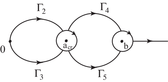
Figure 6: Contour $\Sigma_{R}$

Based on the matching conditions (4.12), (4.13) and the properties of the function $\phi_{t}(z)$ stated in Proposition 4, we have the following estimates:

$$J_{R}(z)=\left\{\begin{array}[]{ll}I+O\left(n^{-1/5}\right),&z\in\partial U(a_{cr},r),\\[2.84544pt] I+O\left(\frac{1}{n}\right),&z\in\partial U(b,r),\\[2.84544pt] I+O(e^{-cn}),{}&z\in\Sigma_{R}\setminus(\partial U(a,r)\cup\partial U(b,r)),\end{array}\right.$$ (4.27)

where $c$ is a positive constant, and the error term is uniform for $z$ on the corresponding contours. Here we also require that $t-t_{cr}=O(n^{-4/5})$; see Remark 4. Then, applying the standard argument of integral operator and using the technique of deformation of contours, see for example [11], we can see that $R(z)$ exits when $n$ is large enough and $t$ is close to $t_{cr}$. Moreover, we have

$$R(z)=I+O(n^{-1/5}),$$ (4.28)

uniformly for $z$ in the whole complex plane.

This completes the nonlinear steepest descent analysis.

5 Proof of the main results

To prove our main results, Theorems 2 and 3, we need more refined asymptotic approximations for $R(z)$ than the one we get in (4.28).

5.1 Asymptotic approximation of $R(z)$

For this purpose, we derive an asymptotic approximation for $R(z)$. To simplify the statement of our result, we denote

$$\sigma_{+}=\left(\begin{array}[]{cc}0&1\\ 0&0\\ \end{array}\right)~{}~{}\mbox{and}~{}~{}\sigma_{-}=\left(\begin{array}[]{cc}0&0\\ 1&0\\ \end{array}\right).$$

Proposition 5.

Let $M=\frac{1}{\sqrt{2}}(I+i\sigma_{1})$ and $\mathcal{H}=\mathcal{H}(n^{4/5}q(z))$; see (1.28). For $n\to\infty$, $t\to t_{cr}$ as in (1.34), and $s^{*}$ is not a pole of the tronquée solution $y_{\alpha}(s)$, we have

$$R(z)=I+M^{-1}\biggl{(}\frac{R^{(1)}(z)}{n^{1/5}}+\frac{R^{(2)}(z)}{n^{2/5}}+O\left(\frac{1}{n^{3/5}}\right)\biggr{)}M,$$ (5.1)

where

$$R^{(1)}(z)=\begin{cases}\displaystyle\frac{r_{1}\mathcal{H}(s^{*})}{z-a_{cr}}\sigma_{-},&z\in\mathbb{C}\setminus U(a_{cr},r),\vspace{2mm}\\ -\displaystyle\frac{i\mathcal{H}}{\varrho^{2}\sqrt{f}}\sigma_{+}+\left(\frac{i\mathcal{H}\varrho^{2}}{\sqrt{f}}+\frac{r_{1}\mathcal{H}(s^{*})}{z-a_{cr}}\right)\sigma_{-},&z\in U(a_{cr},r)\end{cases}$$ (5.2)

and

$$R^{(2)}(z)=\frac{r_{2}}{z-a_{cr}}(y_{\alpha}(s^{*})-\mathcal{H}^{2}(s^{*}))\sigma_{3},\quad z\in\mathbb{C}\setminus U(a_{cr},r).$$ (5.3)

The constants $r_{1}$ and $r_{2}$ in the above formulas are given as

$$r_{1}=-i\biggr{(}2a_{cr}(b_{cr}-a_{cr})\biggl{)}^{\frac{2}{5}},~{}~{}r_{2}=-\displaystyle\frac{a_{cr}^{4/5}}{(2(b_{cr}-a_{cr}))^{1/5}},$$ (5.4)

and $s^{*}=n^{4/5}q(a_{cr})=n^{4/5}(t_{cr}-t)(2a_{cr})^{-\frac{3}{5}}(a_{cr}b_{cr})^{-\frac{1}{2}}(b_{cr}-a_{cr})^{\frac{2}{5}}$, cf. (1.34).

Proof.

From (1.22) and (4.27), we derive an asymptotic expansion for the jump $J_{R}(z)$

$$J_{R}(z)=P^{(a)}(z)N^{-1}(z)=I+\sum_{k=1}^{\infty}\frac{J_{R}^{(k)}(z)}{n^{k/5}},\qquad z\in\partial U(a_{cr},r),$$ (5.5)

where

$$J_{R}^{(k)}(z)=N(z)e^{\pi i\sigma_{3}/4}\,\Psi_{-k}(n^{\frac{4}{5}}q(z))\,e^{-\pi i\sigma_{3}/4}N(z)^{-1}(f(z))^{-k/2},~{}~{}k=1,2,\cdots.$$ (5.6)

For $z\in\partial U(b,r)$, $J_{R}(z)$ is expanded in terms of $n^{-k}$ for non-negative integers $k$. Thus, we have (5.1) for large $n$.

To derive the explicit formulas of $R^{(1)}(z)$ and $R^{(2)}(z)$, we combine (4.25), (5.1) with (5.5). Then one can see that $R^{(1)}(z)$ and $R^{(2)}(z)$ satisfy RH problems as follows:

• $R^{(1)}(z)$ and $R^{(2)}(z)$ are analytic for $z\in\mathbb{C}\setminus\partial U(a_{cr},r)$;

• $R^{(1)}(z)$ and $R^{(2)}(z)$ satisfy the jump conditions

  $$R^{(1)}_{+}(z)-R^{(1)}_{-}(z)=\frac{i\mathcal{H}}{\varrho^{2}\sqrt{f}}\sigma_{+}-\frac{i\mathcal{H}\varrho^{2}}{\sqrt{f}}\sigma_{-},\ z\in\partial U(a_{cr},r)$$ (5.7)

  and

  $$R^{(2)}_{+}(z)-R^{(2)}_{-}(z)=\frac{\mathcal{H}^{2}I+y_{\alpha}\sigma_{3}}{2f}+R_{-}^{(1)}(z)\left(\frac{i\mathcal{H}}{\varrho^{2}\sqrt{f}}\sigma_{+}-\frac{i\mathcal{H}\varrho^{2}}{\sqrt{f}}\sigma_{-}\right),\ z\in\partial U(a_{cr},r),$$ (5.8)

• As $z\to\infty$, both $R^{(1)}(z)$ and $R^{(2)}(z)$ are of order $O(z^{-1})$.

It follows from the Plemelj formula that $R^{(1)}(z)$ and $R^{(2)}(z)$ can be represented as the Cauchy-type integrals on the circular contour $\partial U(a_{cr},r)$ of the right-hand terms in (5.7) and (5.8), respectively. The above RH problems can then be solved by conducting residue calculations of the Cauchy-type integrals. As a direct consequence we obtain (5.2) and (5.3). ∎

5.2 Proof of the main theorems

Now we are ready to derive the large-$n$ asymptotics for the recurrence coefficients and the Hankel determinant, as stated in our main theorems, Theorems 2 and 3.

Proof of Theorems 2 and 3. Tracing back the transformations $R\to S\to T\to Y$ in (4.1), (4.5) and (4.24), we have

$$Y(z)=e^{\frac{nl}{2}\sigma_{3}}R(z)N(z)e^{n(g(z)-\frac{1}{2}l)\sigma_{3}}$$ (5.9)

for $z$ close to the origin. To apply the differential identities (2.8) in Lemma 1, we need to extract the asymptotics of $Y(0)$ when $k=n$, $n\to\infty$, $t\to t_{cr}$ as in (1.34), and $s^{*}$ is not a pole of the tronquée solution $y_{\alpha}(s)$. From the explicit formula of $N(z)$ in (4.11) and the approximation of $R(z)$ in (5.1), we have

$$R(0)N(0)= \frac{1}{2}\left(\begin{array}[]{cc}d+\frac{1}{d}&-i(d-\frac{1}{d})\\ i(d-\frac{1}{d})&d+\frac{1}{d}\\ \end{array}\right)-\frac{r_{1}\mathcal{H}(s^{*})}{2a_{cr}d\,n^{1/5}}\left(\begin{array}[]{cc}-i&1\\ 1&i\\ \end{array}\right)$$ (5.14)

$$-\frac{r_{2}\left(y_{\alpha}(s^{*})-\mathcal{H}^{2}(s^{*})\right)}{2a_{cr}n^{2/5}}\left(\begin{array}[]{cc}\frac{1}{d}-d&i(d+\frac{1}{d})\\ -i(d+\frac{1}{d})&\frac{1}{d}-d\\ \end{array}\right)+O\left(\frac{1}{n^{3/5}}\right),$$ (5.17)

where $d=\left(\frac{b}{a_{cr}}\right)^{1/4}$ and the constants $r_{j}$ are defined in (5.4). Now (2.8) in Lemma 1 implies that

$$\frac{d}{dt}H_{n,n}(t)=-n^{2}(R(0)N(0))_{12}(R(0)N(0))_{21}.$$ (5.18)

Then the asymptotic formula (1.35) for the Hankel determinant follows immediately from the identities (5.14) and (5.18). This completes the proof of Theorem 2.

To derive the asymptotics of the recurrence coefficient $\beta_{n,n}$ and the leading coefficient $\gamma_{n,n}$, we use the relations

$$\beta_{n,n}=(Y_{-1})_{12}(Y_{-1})_{21},\qquad\gamma_{n,n}^{2}=-\frac{1}{2\pi i(Y_{-1})_{12}},$$ (5.19)

where $Y_{-1}$ is the coefficient of the $O(1/z)$ term in the asymptotic expansion of $Y(z)z^{-n\sigma_{3}}$, that is,

$$Y(z)z^{-n\sigma_{3}}=I+\sum_{j=1}^{\infty}\frac{Y_{-j}}{z^{j}}\quad\textrm{as }\ z\to\infty.$$ (5.20)

Therefore, we also need to expand $N(z)$ and $R(z)$ as $z\to\infty.$ Again, using the explicit formula of $N(z)$ in (4.11) and the asymptotic approximation of $R(z)$ in (5.1), we have

$$N(z)=I+\frac{N_{-1}}{z}+O\left(\frac{1}{z^{2}}\right),\quad\textrm{with }N_{-1}=\frac{1}{4}(b-a_{cr})M^{-1}\sigma_{3}M,$$ (5.21)

and

$$R(z)=I+\frac{R_{-1}}{z}+O\left(\frac{1}{z^{2}}\right),$$ (5.22)

where

$$R_{-1}=\frac{r_{1}\mathcal{H}(s^{*})M^{-1}\sigma_{-}M}{n^{1/5}}+\frac{r_{2}(y_{\alpha}(s^{*})-\mathcal{H}(s^{*})^{2})M^{-1}\sigma_{3}M}{n^{2/5}}+O\left(\frac{1}{n^{3/5}}\right).$$ (5.23)

Recalling the values of $r_{1}$ and $r_{2}$ in (5.4), and the identities $M^{-1}\sigma_{-}M=\frac{1}{2}\left(\begin{array}[]{cc}-i&1\\ 1&i\\ \end{array}\right)$ and $M^{-1}\sigma_{3}M=\left(\begin{array}[]{cc}0&i\\ -i&0\\ \end{array}\right)$, we have from (5.9) and (5.19) that

$$\beta_{n,n} =(R_{-1}+N_{-1})_{12}(R_{-1}+N_{-1})_{21}$$

$$=\frac{(b_{cr}-a_{cr})^{2}}{16}-\frac{(2a_{cr}(b_{cr}-a_{cr}))^{4/5}y_{\alpha}(s^{*})}{4}\frac{1}{n^{2/5}}+O\left(\frac{1}{n^{3/5}}\right).$$

This is (1.37).

Similarly, the asymptotics for the leading coefficient can be obtained. Indeed, we have

$$\gamma_{n,n}^{2}= -\frac{e^{-nl}}{2\pi i}\frac{1}{(R_{-1}+N_{-1})_{12}}$$

$$= -\frac{e^{-nl}}{2\pi i}\left(\frac{b_{cr}-a_{cr}}{4}i+\frac{r_{1}\mathcal{H}(s^{*})}{2n^{1/5}}+\frac{ir_{2}(y_{\alpha}(s^{*})-\mathcal{H}(s^{*})^{2})}{n^{2/5}}+O\left(\frac{1}{n^{3/5}}\right)\right)^{-1}$$

$$= \frac{2e^{-nl}}{\pi(b_{cr}-a_{cr})}\left(1-\frac{2ir_{1}\mathcal{H}(s^{*})}{(b_{cr}-a_{cr})n^{1/5}}+\frac{4r_{2}(y_{\alpha}(s^{*})-\mathcal{H}(s^{*})^{2})}{(b_{cr}-a_{cr})n^{2/5}}+O\left(\frac{1}{n^{3/5}}\right)\right)^{-1}$$

$$= \frac{2e^{-nl}}{\pi(b_{cr}-a_{cr})}\biggl{(}1+\frac{2ir_{1}\mathcal{H}(s^{*})}{(b_{cr}-a_{cr})n^{1/5}}$$

$$-\frac{4r_{1}^{2}\mathcal{H}(s^{*})^{2}+4r_{2}(y_{\alpha}(s^{*})-\mathcal{H}(s^{*})^{2})(b_{cr}-a_{cr})}{(b_{cr}-a_{cr})^{2}n^{2/5}}+O\left(\frac{1}{n^{3/5}}\right)\biggr{)},$$ (5.24)

which gives us (1.38).

Finally, we derive the asymptotics for $a_{n,n}$. Note that, from (2.6), we have

$$a_{n,n}=2\pi it\gamma_{n,n}^{2}Y_{11}(0)Y_{12}(0).$$ (5.25)

To find the asymptotic behavior of $Y_{11}(0)Y_{12}(0)$, we have from (5.9) and (5.14) that

$$Y_{11}(0)Y_{12}(0)$$

$$=e^{nl}(R(0)N(0))_{11}(R(0)N(0))_{12}$$

$$=e^{nl}\left\{-\frac{i}{4}\left(d^{2}-d^{-2}\right)-\frac{r_{1}\mathcal{H}(s^{*})}{2\sqrt{a_{cr}b_{cr}}n^{1/5}}\right.$$

$$\quad\left.-i\left(\frac{r_{1}^{2}\mathcal{H}(s^{*})^{2}}{4a_{cr}\sqrt{a_{cr}b_{cr}}}+\frac{r_{2}(y_{\alpha}(s^{*})-\mathcal{H}(s^{*})^{2})(b_{cr}+a_{cr})}{2a_{cr}\sqrt{a_{cr}b_{cr}}}\right)\frac{1}{n^{2/5}}+O\left(\frac{1}{n^{3/5}}\right)\right\}$$

$$=-e^{nl}\frac{(b_{cr}-a_{cr})i}{4\sqrt{a_{cr}b_{cr}}}\left\{1-\frac{2ir_{1}\mathcal{H}(s^{*})}{(b_{cr}-a_{cr})n^{1/5}}\right.$$

$$\quad\left.+\left(\frac{r_{1}^{2}\mathcal{H}(s^{*})^{2}}{a_{cr}(b_{cr}-a_{cr})}+\frac{2r_{2}(y_{\alpha}(s^{*})-\mathcal{H}(s^{*})^{2})(b_{cr}+a_{cr})}{a_{cr}(b_{cr}-a_{cr})}\right)\frac{1}{n^{2/5}}+O\left(\frac{1}{n^{3/5}}\right)\right\}.$$

Then, the asymptotic approximation for $a_{n,n}$ in (1.36) follows from the above formula and (5.2).

This completes the proof of Theorem 3. ∎

References

- [1] M.R. Atkin, T. Claeys and F. Mezzadri, Random matrix ensembles with singularities and a hierarchy of Painlevé III equations, preprint, arXiv:1501.04475.
- [2] M. Bertola, B. Eynard and J. Harnad, Semiclassical orthogonal polynomials, matrix models and isomonodromic tau functions, Comm. Math. Phys., 263(2006), 401-437.
- [3] M. Bertola, B. Eynard and J. Harnad, Partition functions for matrix models and isomonodromic tau functions. Random matrix theory, J. Phys. A, 36(2003), 3067-3083.
- [4] M. Bertola and A. Tovbis, Asymptotics of orthogonal polynomials with complex varying quartic weight: global structure, critical point behaviour and the first Painlevé equation, Constr. Approx., 41(2015), 529-587.
- [5] P.M. Bleher and A. Deaño, Topological expansion in the cubic random matrix model, Int. Math. Res. Not., 2013(2013), 2699-2755.
- [6] P.M. Bleher and A. Deaño, Painlevé I double scaling limit in the cubic matrix model, arXiv:1310.3768.
- [7] L. Brightmore, F. Mezzadri and M.Y. Mo, A matrix model with a singular weight and Painlevé III, Comm. Math. Phys., 333(2015), 1317-1364.
- [8] P.W. Brouwer, K.M. Frahm and C.W.J. Beenakker, Quantum mechanical time-delay matrix in chaotic scattering, Phys. Rev. Lett., 78(1997), 4737-4740.
- [9] Y. Chen and A. Its, Painlevé III and a singular linear statistics in Hermitian random matrix ensembles. I, J. Approx. Theory, 162(2010), 270-297.
- [10] T. Claeys and A.B.J. Kuijlaars, Universality of the double scaling limit in random matrix models, Comm. Pure Appl. Math., 59(2006), 1573-1603.
- [11] P. Deift, Orthogonal polynomials and random matrices: a Riemann-Hilbert approach, Courant Lecture Notes 3, New York University, 1999.
- [12] P. Deift, T. Kriecherbauer, K.T.-R. McLaughlin, S. Venakides and X. Zhou, Uniform asymptotics for polynomials orthogonal with respect to varying exponential weights and applications to universality questions in random matrix theory, Comm. Pure Appl. Math., 52(1999), 1335-1425.
- [13] P. Deift, T. Kriecherbauer, K.T.-R. McLaughlin, S. Venakides and X. Zhou, Strong asymptotics of orthogonal polynomials with respect to exponential weights, Comm. Pure Appl. Math., 52(1999), 1491-1552.
- [14] M. Duits and A.B.J. Kuijlaars, Painlevé I asymptotics for orthogonal polynomials with respect to a varying quartic weight, Nonlinearity, 19(2006), 2211-2245.
- [15] L. Eisenbud, Formal properties of nuclear collisions, Ph.D. thesis, Princeton University, 1948.
- [16] A.S. Fokas, A.R. Its and A.V. Kitaev, Discrete Painlevé equations and their appearance in quantum gravity, Comm. Math. Phys., 142(1991) 313-344.
- [17] A.S. Fokas, A.R. Its and A.V. Kitaev, The isomonodromy approach to matrix models in 2D quantum gravity, Comm. Math. Phys., 147(1992), 395-430.
- [18] A.S. Fokas, A.R. Its, A.A. Kapaev and V.Yu. Novokshenov, Painlevé transcendents: the Riemann-Hilbert approach, AMS Mathematical Surveys and Monographs, Vol. 128, Amer. Math. Soc., Providence R.I., 2006.
- [19] M. Jimbo, T. Miwa and K. Ueno, Monodromy preserving deformation of linear ordinary differential equations with rational coefficients. I. General theory and -function, Phys. D, 2(1981), 306-352.
- [20] N. Joshi and A.V. Kitaev, On Boutroux’s tritronquée solutions of the first Painlevé equation, Stud. Appl. Math., 107(2001), 253–291.
- [21] A.A. Kapaev, Quasi-linear Stokes phenomenon for the Painlevé first equation, J. Phys. A, 37(2004), 11149-11167.
- [22] F. Olver, D. Lozier, R. Boisvert and C. Clark, NIST handbook of mathematical functions, Cambridge University Press, Cambridge, 2010.
- [23] V.A. Osipov and E. Kanzieper, Are bosonic replicas faulty? Phys. Rev. Lett., 99(2007), 050602.
- [24] E.B. Saff and V. Totik, Vilmos, Logarithmic potentials with external fields, Grundlehren der Mathematischen Wissenschaften vol. 316, Springer-Verlag, Berlin, 1997.
- [25] F.T. Smith, Lifetime matrix in collision theory, Phys. Rev., 118(1960), 349-356.
- [26] G. Szegő, Orthogonal polynomials, Fourth Edition, Colloquium Publications Vol. 23, Amer. Math. Soc., Providence, R.I., 1975.
- [27] C. Texier and S.N. Majumdar, Wigner time-delay distribution in chaotic cavities and freezing transition, Phys. Rev. Lett., 110(2013), 250602.
- [28] M. Vanlessen, Strong asymptotics of Laguerre-type orthogonal polynomials and applications in random matrix theory, Constr. Approx., 25(2007), 125-175.
- [29] E.P. Wigner, Lower limit for the energy derivative of the scattering phase shift, Phys. Rev., 98(1955). 145-147.
- [30] S.-X. Xu, D. Dai and Y.-Q. Zhao, Critical edge behavior and the Bessel to Airy transition in the singularly perturbed Laguerre unitary ensemble, Comm. Math. Phys., 332(2014), 1257-1296.
- [31] S.-X. Xu, D. Dai and Y.-Q. Zhao, Painlevé III asymptotics of Hankel determinants for a singularly perturbed Laguerre weight, J. Approx. Theory, 192(2015), 1-18.