Testing separability of space–time functional processes

Abstract

We present a new methodology and accompanying theory to test for separability of spatio–temporal functional data. In spatio–temporal statistics, separability is a common simplifying assumption concerning the covariance structure which, if true, can greatly increase estimation accuracy and inferential power. While our focus is on testing for the separation of space and time in spatio-temporal data, our methods can be applied to any area where separability is useful, including biomedical imaging. We present three tests, one being a functional extension of the Monte Carlo likelihood method of [2005], while the other two are based on quadratic forms. Our tests are based on asymptotic distributions of maximum likelihood estimators, and do not require Monte Carlo or bootstrap replications. The specification of the joint asymptotic distribution of these estimators is the main theoretical contribution of this paper. It can be used to derive many other tests. The main methodological finding is that one of the quadratic form methods, which we call a norm approach, emerges as a clear winner in terms of finite sample performance in nearly every setting we considered. The norm approach focuses directly on the Frobenius distance between the spatio–temporal covariance function and its separable approximation. We demonstrate the efficacy of our methods via simulations and an application to Irish wind data.

1 Introduction

The assumption of separability is used heavily in spatio–temporal statistics, [1995], [2007], [2011], [2011], [2012], among many others. It is introduced in many textbooks, e.g. [2005], [2011]. Separability means that the spatio–temporal covariance structure factors into the product of two functions, one depending only on space, the other only on time. Such an assumption provides a number of benefits. From a modeling perspective, it allows one to draw on the large literature on covariance structures for spatial or temporal data. The simpler structure induced by separability is then much easier to estimate than a nonseparable structure. In the context of multivariate spatio–temporal data, the separability assumption can be stated in terms of the factorization of the covariance matrix. For more complex spatio–temporal data structures, analogous definitions can be formulated, as we explain below. The work presented in this paper is motivated by geostatistical functional data; functions are observed at a number of spatial locations, though our methods can be readily generalized to a number of areas. For example, in biomedical imaging, such as fMRI, one often has data in both space (the brain) and time, separability can greatly simplify modeling. In our context, separability implies that the optimal functions used for (temporal) dimension reduction are the same at every spatial location; information can then be pooled across spatial locations to get very good estimates of these functions. Geostatistical functional data are quite common. Perhaps the best known example is provided by annual temperature and log–precipitation curves (averaged over several decades) at several dozen locations in Canada. These data have been used in many examples in the monograph of of [2005] and many research papers that followed, [2010] provide further references. Our own work has been concerned with such data as well; [2012] and Gromenko and Kokoszka (?, ?) study curves describing the evolution of certain ionospheric parameters measured at globally distributed locations at which radar–type instruments called ionosondes operate. In [2015], we study precipitation measurements extending over several decades at about sixty locations in the Midwest.

Tests of separability for spatio–temporal covariances of scalar fields are reviewed in Mitchell et al. (?, ?) and [2006]. If the spatio–temporal covariance has a specific parametric form, a likelihood ratio test is possible. A similar parametric approach, in conjunction with bootstrap, is taken by [2014] in the context of functional data. [2006] introduce a more general, nonparametric LRT test, which requires that the number of repeated measurements be greater than the product of the number of spatial and temporal locations. We explain their idea in greater detail in the following. [2005] explain how to deal with this restrictions by dividing the temporal domain into blocks. The test of [2006] is based on the spectral representation which assumes that the data are available on a spatial grid. The data that motivate this research are not of this form.

We now explain the contribution of this paper in more specific terms. It is instructive to begin by summarizing the procedure of [2006]. Suppose we observe $N$ iid scalar fields at temporal points $t_{i}$ and spatial locations $s_{k}$, so that the data are replications of the spatio–temporal observations:

$$X_{n}({\bf s}_{k};t_{i}),\ \ \ 1\leq k\leq K,\ \ 1\leq i\leq I.$$

The iid assumption implies that the mean function $EX_{n}({\bf s};t)=\mu({\bf s};t)$ is the same for each replication. The covariances

$$\sigma_{k\ell;ij}=E\left\{\left[X_{n}({\bf s}_{k};t_{i})-\mu({\bf s}_{k};t_{i})\right]\left[X_{n}({\bf s}_{\ell};t_{j})-\mu({\bf s}_{\ell};t_{j})\right]\right\}$$

do not depend on $n$ either. The assumption of separability implies that $\sigma_{k\ell;ij}=u_{k\ell}v_{ij},$ where $u_{kl}$ does not depend on $t$ (time) and $v_{ij}$ does not depend on ${\bf s}$ (space). This relation stated in the matrix form as

(1.1) $${\boldsymbol{\Sigma}}={\bf V}\otimes{\bf U}=\begin{bmatrix}v_{11}{\bf U}&v_{12}{\bf U}&\ldots&v_{1I}{\bf U}\\ v_{21}{\bf U}&v_{22}{\bf U}&\ldots&v_{2I}{\bf U}\\ \vdots&\vdots&\vdots&\vdots\\ v_{I1}{\bf U}&v_{I2}{\bf U}&\ldots&v_{II}{\bf U}\\ \end{bmatrix},$$

where ${\bf U}$ is the $K\times K$ matrix with entries $u_{k\ell}$ and ${\bf V}$ is the $I\times I$ matrix with entries $v_{ij}$. The matrix ${\boldsymbol{\Sigma}}$ is $KI\times KI$ and can be viewed as the covariance matrix of the vectorized matrix $\{X_{n}(s_{k},t_{i})\}$ (with $k$ indexing rows and $i$ columns). [2006] use the test statistic

(1.2) $$\widehat{T}=N\left\{K\log\det[\widehat{\bf V}]+I\log\det[\widehat{\bf U}]-\log\det[\widehat{\boldsymbol{\Sigma}}]\right\},$$

where $\widehat{\bf V},\widehat{\bf U},\widehat{\boldsymbol{\Sigma}}$ are Gaussian likelihood estimates defined in Theorem 2.1. Their approach is based on Theorem 1.1 which justifies a Monte Carlo approximation for the null distribution of $\widehat{T}$. One can, e.g., use $\mu=0,{\bf U}={\bf I}_{K},{\bf V}={\bf I}_{I}$ to obtain a large number of replicates of $\widehat{T}$, and so approximate its null distribution.

Theorem 1.1 ([2006]).

If the observations are normal, (1.1) holds, and $N>KI,$ then the distribution of $\widehat{T}$ defined in (1.2) does not depend on $\mu,{\bf U},{\bf V}$.

The choice of statistic (1.2) is thus fundamentally justified by the invariance property stated in Theorem 1.1. Perhaps more natural test statistics should be based on some distance between the matrices $\widehat{\boldsymbol{\Sigma}}$ and $\widehat{\bf V}\otimes\widehat{\bf U}$. It might be hoped that a more direct comparison would lead to tests with better power. However, such statistics are not invariant in the sense of Theorem 1.1 and their asymptotic distribution has not been found. The first contribution of this paper is to derive the joint asymptotic null distribution of $\widehat{\boldsymbol{\Sigma}},\widehat{\bf V},\widehat{\bf U}$ and show how it enables to derive the limit distribution a several natural test statistic in the multivariate context. This is addressed in Section 2. The proofs are presented in the Appendix.

The second contribution, which motivated our research, is related to functional data which are $N$ replications of the field

$$X_{n}({\bf s}_{k},t),\ \ 1\leq k\leq K,\ \ t\in{\mathcal{T}}.$$

At each spatial location ${\bf s}_{k}$, a function with argument $t$ is observed. For example, $X_{n}({\bf s}_{k},t)$ can be the maximum daily temperature on day $t$ of year $n$ at location ${\bf s}_{k}$. For historical climate and environmental data sets of this type, $N$ is about 100, $K$ can be anything from several dozen to a few hundred, and the number of measurements per year is $I=365$. The approach of [2006] thus cannot be applied because the condition $N>KI$ is violated. One cannot subdivide the years into smaller units because the assumption of the identical distribution would be violated, so the modification of [2005] cannot be applied. Our approach exploits the functional structure of the data and uses a dimension reduction. Since for historical climate and environmental data sets $N$ is fairly large, we derive asymptotic tests as $N\to\infty$ using the results of Section 2. These developments are described in Section 3.

The only related work we are aware of which also concerns functional data is given in the (currently) unpublished work of [Aston et al. (2015)]. Since both papers, developed independently and concurrently, are currently unpublished, it is only appropriate to discuss differences and similarities, refraining from any evaluative statements. Both papers aim at solving the same problem, with motivation coming from different data structures. Our work is motivated by geostatistical functional data, curves observed at irregularly distributed spatial locations; [Aston et al. (2015)] are motivated by data observed on grids with one dimension which can be called space and the other time. In their application to phonetic data, space is frequency. Our approach is based on the joint asymptotic distribution of the MLE’s, followed, as an option, by dimension reduction; [Aston et al. (2015)] first perform dimension reduction in space and time which allows them to compute their tests statistic without estimating the full spatio–temporal covariance. Our method uses an approximation via limiting distributions; they use bootstrap approximations. The computational efficiency is thus obtained in very different ways. Regarding asymptotic theory, ours is based on joint MLE’s which require an iterative procedure to compute; [Aston et al. (2015)] compute the marginal space and time covariances by integrating out the other dimension, and then apply the CLT to the difference projected on a finite number of tensor products.

The remainder of this paper is organized as follows. Section 4 compares the finite sample performance of the tests derived Section 3. We show that a test related to a norm of the difference $\widehat{\boldsymbol{\Sigma}}-\widehat{\bf V}\otimes\widehat{\bf U}$ has correct size and is most powerful. It is also more powerful than a Monte Carlo test based on Theorem 1.1 (with a suitable extension to functional data). We apply the tests to an extensively studied Irish wind data set, and confirm the conjecture of T. Gneiting that these space–time data are not separable.

2 Multivariate theory

This section clarifies the behavior of several test statistics based on normal maximum likelihood estimators. The theory is valid under the following assumption.

Assumption 2.1.

Assume ${\bf X}_{1},\ldots,{\bf X}_{N}$ are iid normally distributed $K\times I$ matrices with $\operatorname{E}[{\bf X}_{n}]={\bf M}$ and $\operatorname{Cov}(\operatorname{vec}({\bf X}_{n}))={\boldsymbol{\Sigma}}$, where ${\boldsymbol{\Sigma}}$ is an $KI\times KI$ matrix of full rank.

We begin with Theorem 2.1 whose proof is based on direct, but lengthy and tedious calculations of Gaussian likelihoods for vectorized matrices of various dimensions and solving score equations. It is placed in the supplement. Recall that if ${\bf A}$ is a $K\times I$ matrix, then $\operatorname{vec}({\bf A})$ is a column vector of length $KI$ obtained by stacking the columns of ${\bf A}$ on top of each other.

Theorem 2.1.

Under Assumption 2.1, the maximum likelihood estimators of ${\bf M}$ and ${\boldsymbol{\Sigma}}$ are

$$\widehat{\bf M}=\frac{1}{N}\sum_{n=1}^{N}{\bf X}_{n},\ \ \ \ \widehat{\boldsymbol{\Sigma}}=\frac{1}{N}\sum_{n=1}^{N}\operatorname{vec}({\bf X}_{n}-\widehat{\bf M})(\operatorname{vec}({\bf X}_{n}-\widehat{\bf M}))^{\top}.$$

If ${\boldsymbol{\Sigma}}$ admits the decomposition

(2.1) $${\boldsymbol{\Sigma}}={\bf V}\otimes{\bf U},\ \ \ {\rm dim}({\bf U})=K\times K,\ \ {\rm dim}({\bf V})=I\times I,$$

where ${\bf U}$ and ${\bf V}$ are of full rank, then the maximum likelihood estimators of ${\bf U}$ and ${\bf V}$ satisfy

$$\widehat{\bf U} =\frac{1}{NI}\sum_{n=1}^{N}({\bf X}_{n}-\widehat{\bf M}){\widehat{\bf V}}^{-1}({\bf X}_{n}-\widehat{\bf M})^{\top}$$

$$\widehat{\bf V} =\frac{1}{NK}\sum_{n=1}^{N}({\bf X}_{n}-\widehat{\bf M})^{\top}{\widehat{\bf U}}^{-1}({\bf X}_{n}-\widehat{\bf M}).$$

The estimators $\widehat{\bf U}$ and $\widehat{\bf V}$ are defined indirectly and must be computed using an iterative procedure with some normalization to ensure identifiability. The following algorithm, [1999], produces $O_{P}(N^{-1/2})$ consistent estimators. It uses the normalization $\operatorname{tr}({\bf U}_{i})=K$.

Algorithm 2.1.

Initialize with ${\bf U}_{0}={\bf I}_{K}$ ($K\times K$ identity matrix). For $i=0,1,2,\ldots$ calculate

$$\widehat{\bf V}_{i} =\frac{1}{NK}\sum_{n=1}^{N}({\bf X}_{n}-\widehat{\bf M})^{\top}{\widehat{\bf U}}_{i}^{-1}({\bf X}_{n}-\widehat{\bf M}),$$

$$\widetilde{\bf U}_{i+1} =\frac{1}{NI}\sum_{n=1}^{N}({\bf X}_{n}-\widehat{\bf M}){\widehat{\bf V}}_{i}^{-1}({\bf X}_{n}-\widehat{\bf M})^{\top},$$

$$\widehat{\bf U}_{i+1} =\frac{K}{\operatorname{tr}(\widetilde{\bf U}_{i+1})}\widetilde{\bf U}_{i+1},$$

until convergence is reached.

The most natural statistic to test separability, i.e. ${\boldsymbol{\Sigma}}={\bf V}\otimes{\bf U}$, should be based on a difference between $\widehat{\bf V}\otimes\widehat{\bf U}$ and $\widehat{\boldsymbol{\Sigma}}$. We will show that the statistic

$$\widehat{T}_{F}=N\|\widehat{\bf V}\otimes\widehat{\bf U}-\widehat{\boldsymbol{\Sigma}}\|_{F}^{2},$$

where $\|\cdot\|_{F}^{2}$ is the squared Frobenius matrix norm (i.e. the sum of squares of all entries), converges, and find the asymptotic distribution. This distribution involves the asymptotic covariance matrix of $\operatorname{vec}(\widehat{\bf V}\otimes\widehat{\bf U}-\widehat{\boldsymbol{\Sigma}})$, which we denote by ${\bf W}$. The form of ${\bf W}$ is complex, see (B.1). To obtain a chi–square limit distribution, a suitable quadratic form must be used. This leads to the statistic

$$\widehat{T}_{W}=N\operatorname{vec}(\widehat{\bf V}\otimes\widehat{\bf U}-\widehat{\boldsymbol{\Sigma}})^{\top}\widehat{\bf W}^{+}\operatorname{vec}(\widehat{\bf V}\otimes\widehat{\bf U}-\widehat{\boldsymbol{\Sigma}}),$$

where $\widehat{\bf W}$ is an estimator of ${\bf W}$ and $\widehat{\bf W}^{+}$ is its generalized inverse. A generalized inverse must be used because ${\bf U}$, ${\bf V}$, and ${\boldsymbol{\Sigma}}$ (and the corresponding estimates) are all symmetric, and this implies many linear constraints, $\hat{U}_{k\ell}=\hat{U}_{\ell k}$ for example, on the entries of $\operatorname{vec}(\widehat{\bf V}\otimes\widehat{\bf U}-\widehat{\boldsymbol{\Sigma}})$ and so of $\widehat{\bf W}$. Using a generalized inverse is equivalent to dropping redundant entries.

We will also show that the likelihood ratio statistic

$$\widehat{T}_{L}=N\left(T\log\det(\widehat{\bf U})+K\log\det(\widehat{\bf V})-\log\det(\widehat{\boldsymbol{\Sigma}})\right)$$

discussed in Section 1 has the same limit as $\widehat{T}_{W}$, i.e. is asymptotically chi–square with a known number of degrees of freedom. The asymptotic chi–square distribution of $\widehat{T}_{L}$ was claimed by [2005] without proof. We present a detailed proof in Section B. [2006] did not use this asymptotic result; they utilized a Monte Carlo finite sample approximation based on Theorem 1.1. We collect our results in Theorem 2.2.

Theorem 2.2.

Suppose Assumption 2.1 and decomposition (2.1) hold. Let ${\bf W}$ be the $KI\times KI$ matrix defined in (B.1), with $\gamma_{1},\gamma_{2},\dots,\gamma_{R}$ its eigenvalues. Then, as $N\to\infty$,

$$\widehat{T}_{L}\sim\chi^{2}_{d}\quad\mbox{and}\quad\widehat{T}_{W}\sim\chi^{2}_{d}$$

where

$$d=\frac{KI(KI+1)}{2}-\frac{K(K+1)}{2}-\frac{I(I+1)}{2}+1,$$

and

$$\widehat{T}_{F}\sim\sum_{r=1}^{R}\gamma_{r}\chi^{2}_{1}(r),$$

where $\{\chi^{2}_{1}(r)\}$ are iid chi-square random variables with one degree of freedom.

Theorem 2.2 is proven in Section B. The three statistics listed in Theorem 2.2 are not the only ones that our theory covers. Theorem B.1, which specifies the joint asymptotic distribution of $\widehat{\bf V},\widehat{\bf U}$ and $\widehat{\boldsymbol{\Sigma}}$, can be used to derive the asymptotic distribution of many other reasonable test statistics.

3 Tests for functional data

We now show how the results of Section 2 are applied to testing separability of geostatistical functional data. For a reader interested in learning more about functional data methods there are now several introductory books including [2005, 2009, 2012, 2015]. We consider independent spatio–temporal random fields $X_{n}(\cdot,\cdot),1\leq n\leq N,$ which have the same distribution as the field $\left\{X({\bf s},t),{\bf s}\in{\mathcal{S}},t\in{\mathcal{T}}\right\}$, which satisfies $E\int_{{\mathcal{S}}}\int_{\mathcal{T}}X^{2}({\bf s},t)d{\bf s}dt<\infty.$ Then $X_{n}({\bf s},t)=\mu({\bf s},t)+\varepsilon_{n}({\bf s},t),$ where $\mu\in L^{2}({\mathcal{S}}\times{\mathcal{T}})$, and the $\varepsilon_{n}$ are iid random elements of $L^{2}({\mathcal{S}}\times{\mathcal{T}})$ which satisfy

$$E\int_{{\mathcal{S}}}\int_{\mathcal{T}}\varepsilon_{n}^{2}({\bf s},t)d{\bf s}dt<\infty\ \ \ {\rm and}\ \ \ E\varepsilon_{n}({\bf s},t)=0.$$

We consider the covariances

$$\sigma({\bf s},{\bf s}^{\prime};t,t^{\prime})=\operatorname{Cov}(X({\bf s},t),X({\bf s}^{\prime},t^{\prime}))=E[\varepsilon_{n}({\bf s};t)\varepsilon_{n}({\bf s}^{\prime},t^{\prime})].$$

Our objective is to test

(3.1) $$H_{0}:\ \ \ \sigma({\bf s},{\bf s}^{\prime};t,{t^{\prime}})={\mathcal{U}}({\bf s},{\bf s}^{\prime}){\mathcal{V}}(t,{t^{\prime}}).$$

As in the multivariate case, the functions ${\mathcal{U}}$ and ${\mathcal{V}}$ are uniquely determined only up to multiplicative constants, and a testing algorithm must include some arbitrary normalization. However, the P–values of our testing procedures do not depend on this choice. We now proceed with the description of test procedures of increasing complexity.

3.1 Procedure 1: fixed spatial locations, fixed temporal basis

We assume that for each $n$ the field $X_{n}$ is observed at the same spatial locations ${\bf s}_{k},1\leq k\leq K$. We estimate $\mu({\bf s}_{k},t)$ by the sample average $\hat{\mu}({\bf s}_{k},t)=N^{-1}\sum_{n=1}^{N}X_{n}({\bf s}_{k},t),$ and focus in the following on the covariance structure. Under $H_{0}$, the covariances of the observations are

$$\operatorname{Cov}(X_{n}({\bf s}_{k},t)X_{n}({\bf s}_{\ell},{t^{\prime}}))=U(k,\ell){\mathcal{V}}(t,{t^{\prime}}),$$

with entries $U(k,\ell)={\mathcal{U}}({\bf s}_{k},{\bf s}_{\ell})$ forming a $K\times K$ matrix ${\bf U}$, and $\mathcal{V}$ being the temporal covariance function over ${\mathcal{T}}\times{\mathcal{T}}$. As in the multivariate setting, the estimation of the matrix ${\bf U}$ and the covariance function ${\mathcal{V}}$ must involve an iterative procedure. In the functional setting, a dimension reduction is also needed. Suppose $\{v_{j},j\geq 1\}$ is a basis system in $L^{2}({\mathcal{T}})$ such that for sufficiently large $J$, the functions

$$X_{n}^{(J)}({\bf s}_{k},t)=\mu({\bf s}_{k},t)+\sum_{j=1}^{J}\xi_{jn}({\bf s}_{k})v_{j}(t)$$

are good approximations to the functions $X_{n}({\bf s}_{k})$. We thus replace a large number of time points by a moderate number $J$, and seek to reduce the testing of $H_{0}$ (3.1) to testing the separability of the covariances of the transformed observations given as $K\times J$ matrices

(3.2) $$\mbox{\boldmath${\Xi}$}_{n}=[\xi_{jn}({\bf s}_{k}),\ 1\leq k\leq K,\ 1\leq j\leq J].$$

The index $j$ should be viewed as a transformed time index. The number $I$ of the actual time points $t_{i}$ can be very large, $J$ is usually much smaller. The following proposition is easy to prove. It establishes the connection between the testing problem (3.1) and testing the separability of the transformed data (3.2). The assumption that the $v_{j}$ are orthonormal cannot be removed.

Proposition 3.1.

For some orthonormal $v_{j}$, set

$$X^{(J)}({\bf s}_{k},t)=\mu({\bf s}_{k},t)+\sum_{j=1}^{J}\xi_{j}({\bf s}_{k})v_{j}(t).$$

If

(3.3) $$E[\xi_{j}({\bf s}_{k})\xi_{i}({\bf s}_{\ell})]=U(k,\ell)V(j,i),$$

then

(3.4) $$\operatorname{Cov}(X^{(J)}({\bf s}_{k},t),X^{(J)}({\bf s}_{\ell},s))=U(k,\ell){\mathcal{V}}(t,s).$$

Conversely, (3.4) implies (3.3). The entries $V(j,i)$ and ${\mathcal{V}}(t,s)$ are related via

$$V(j,i)=\iint{\mathcal{V}}(t,s)v_{j}(t)v_{i}(s)dtds,\ \ \ {\mathcal{V}}(t,s)=\sum_{j,i=1}^{J}V(j,i)v_{j}(t)v_{i}(s).$$

We assume that $\left\{v_{j},\ 1\leq j\leq J\right\}$ is a fixed orthonormal system, for example the first $J$ trigonometric basis functions. Slightly abusing notation, consider the matrices

$$\widehat{\boldsymbol{\Sigma}}\ (KJ\times KJ),\ \ \ \widehat{\bf U}\ (K\times K),\ \ \ \widehat{\bf V}\ (J\times J),$$

defined as in Theorem 2.1, but with matrices ${\bf X}_{n}$ replaced by the matrices $\mbox{\boldmath${\Xi}$}_{n}$. The index $j\leq J$ now plays the role of the index $i\leq I$ of Section 2. To apply tests based on Theorem 2.2, we must recursively calculate $\widehat{\bf U}$ and $\widehat{\bf V}$ using the relations stated in Theorem 2.1. This can be done using Algorithm 2.1 with $\mbox{\boldmath${\Xi}$}_{n}$ in place of ${\bf X}_{n}$. This approach leads to the following test procedure. The test statistic can be one of the three statistics introduced in Section 2.

Procedure 3.1.

1. Choose a deterministic orthonormal basis $v_{j},j\geq 1$.

2. Approximate each curve $X_{n}({\bf s}_{k},t)$ by

$$X_{n}^{(J)}({\bf s}_{k},t)=\hat{\mu}({\bf s}_{k},t)+\sum_{j=1}^{J}\xi_{jn}({\bf s}_{k})v_{j}(t).$$

Construct $K\times J$ matrices $\mbox{\boldmath${\Xi}$}_{n}$ defined in (3.2).

3. Compute the matrix

$$\widehat{\boldsymbol{\Sigma}}=\frac{1}{N}\sum_{n=1}^{N}\operatorname{vec}(\mbox{\boldmath${\Xi}$}_{n}-\widehat{\bf M})(\operatorname{vec}(\mbox{\boldmath${\Xi}$}_{n}-\widehat{\bf M}))^{\top},\ \ \ \ \widehat{\bf M}=\frac{1}{N}\sum_{n=1}^{N}\mbox{\boldmath${\Xi}$}_{n}.$$

Using Algorithm 2.1 with $\mbox{\boldmath${\Xi}$}_{n}$ in place of ${\bf X}_{n}$, compute the matrices $\widehat{\bf U}$ and $\widehat{\bf V}$.

4. Estimate the matrix ${\bf W}$ defined by (B.1) by replacing ${\boldsymbol{\Sigma}},{\bf U},{\bf V}$ by their estimates.

5. Calculate the P–value using the limit distribution specified in Theorem 2.2, with $I$ replaced by $J$.

Step 2 can be easily implemented using R function pca.fd, see [2009]. Several methods of choosing $J$ are available; we used the cumulative variance rule requiring that $J$ be so large that at least 80% of variance is explained for each location ${\bf s}_{k}$.

3.2 Procedure 2: fixed spatial locations, data driven temporal basis

In Section 3.1, we used a deterministic orthonormal system. To achieve the most efficient dimension reduction, it is usual to project on a data driven system, with the functional principal components being used most often. Since the sequences of functions are defined at a number of spatial locations, it is not a priori clear how a suitable orthonormal system should be constructed, as each sequence $\left\{X_{n}({\bf s}_{k}),1\leq n\leq N\right\}$ has different functional principal components $v_{j}({\bf s}_{k}),j\geq 1$, and Proposition 3.1 requires that a single system be used. Our next algorithm proposes an approach which leads to suitable estimates $\widehat{\bf U},\widehat{\bf V}$ and $\widehat{\boldsymbol{\Sigma}}$. It is not difficult to show that these estimators are $O_{P}(N^{-1/2})$ consistent.

Algorithm 3.1.

Initialize with ${\bf U}_{0}={\bf I}_{K}$.

For $i=1,2,\dots$, perform the following two steps until convergence is reached.

1. Calculate

$${\mathcal{V}}_{i}(t,{t^{\prime}})=(NK)^{-1}\sum_{n=1}^{N}(X_{n}(\cdot,t)-\hat{\mu}(\cdot,t))^{\top}{\bf U}_{i-1}^{-1}(X_{n}(\cdot,{t^{\prime}})-\hat{\mu}(\cdot,{t^{\prime}})).$$

Denote the eigenfunctions and eigenvalues of ${\mathcal{V}}_{i}$ by $\{v_{ij}\}$ and $\{\lambda_{ij}\}$. Determine $J_{i}$ such that the first $J_{i}$ eigenfunctions of ${\mathcal{V}}_{i}$ explain at least 85% of the variance.

2. Project each function $X_{n}({\bf s}_{k},\cdot)$ on the first $J_{i}$ eigenfunctions of $\mathcal{V}_{i}$. Denote the scores of these projections by

$$Z_{in}({\bf s}_{k},j)=\langle X_{n}({\bf s}_{k},\cdot)-\hat{\mu}({\bf s}_{k},\cdot),v_{ij}\rangle$$

and calculate

$$U_{i}(k,\ell)=(NJ_{i})^{-1}\sum_{j=1}^{J_{i}}\sum_{n=1}^{N}\frac{Z_{in}({\bf s}_{k},j)Z_{in}({\bf s}_{\ell},j)}{\lambda_{ij}}.$$

Normalize ${\bf U}_{i}$ so that $\operatorname{tr}({\bf U}_{i})=K$.

Let $\{\hat{v}_{j},1\leq j\leq J\}$ denote the final eigenfunctions. Carry out the final projection $\hat{Z}_{n}({\bf s}_{k},j)=\langle X_{n}({\bf s}_{k},\cdot)-\hat{\mu}({\bf s}_{k},\cdot),\hat{v}_{j}\rangle$. For each $n$, denote by $\widehat{\bf Z}_{n}$ the $K\times J$ matrix with these entries. Set

(3.5) $$\widehat{\boldsymbol{\Sigma}}=\frac{1}{N}\sum_{n=1}^{N}\operatorname{vec}(\widehat{\bf Z}_{n})\operatorname{vec}(\widehat{\bf Z}_{n})^{\top}$$

and apply Algorithm 2.1 with ${\bf X}_{n}=\widehat{\bf Z}_{n}$ to obtain $\widehat{\bf U}$ and $\widehat{\bf V}$.

Using the above algorithm, the testing procedure is as follows:

Procedure 3.2.

1. Calculate matrices $\widehat{\boldsymbol{\Sigma}},\widehat{\bf U},\widehat{\bf V}$ according to Algorithm 3.1.

2. Perform steps 4 and 5 of Procedure 3.1.

3.3 Procedure 3: dimension reduction in both space and time

Similar with Procedure 1 we assume that for each $n$ the field $X_{n}$ is observed at the same spatial locations ${\bf s}_{k},1\leq k\leq K$. We estimate $\mu({\bf s}_{k},t)$ by the sample average $\hat{\mu}({\bf s}_{k},t)=N^{-1}\sum_{n=1}^{N}X_{n}({\bf s}_{k},t),$ and focus in the following on the covariance structure. Under $H_{0}$, the covariances of the observations are

$$\operatorname{Cov}(X_{n}({\bf s}_{k},t)X_{n}({\bf s}_{\ell},{t^{\prime}}))=U(k,\ell){\mathcal{V}}(t,{t^{\prime}}),$$

with entries $U(k,\ell)={\mathcal{U}}({\bf s}_{k},{\bf s}_{\ell})$ forming a $K\times K$ matrix ${\bf U}$, and $\mathcal{V}$ being the temporal covariance function over ${\mathcal{T}}\times{\mathcal{T}}$.

The testing procedure for dimension reduction in both space and time is as follows:

Procedure 3.3.

1. Choose a deterministic orthonormal basis $v_{j},j\geq 1$.

2. Approximate each curve $X_{n}({\bf s}_{k},t)$ by

$$X_{n}^{(J)}({\bf s}_{k},t)=\hat{\mu}({\bf s}_{k},t)+\sum_{j=1}^{J}\xi_{jn}({\bf s}_{k})v_{j}(t).$$

Construct $K\times J$ matrices $\mbox{\boldmath${\Xi}$}_{n}$ defined in (3.2) where $J$ is chosen so large that for each $k$ the first $J$ sample eigenvalues explain at least $80\%$ of the variance. This is Functional Principal Components Analysis carried out on the pooled (across space) sample.

3. Approximate each vector $(\xi_{jn}({\bf s}_{1}),\dots,\xi_{jn}({\bf s}_{K}))$ using

$$\xi_{jn}({\bf s}_{k})=\sum_{l=1}^{L}\zeta_{lj;n}u_{l}(s_{k}).$$

The vectors $(u_{l}(s_{1}),\dots,u_{l}(s_{K}))$ are the eigenvectors of the following matrix

$$\tilde{U}_{i}(k,\ell)=(NJ_{i})^{-1}\sum_{j=1}^{J_{i}}\sum_{n=1}^{N}\frac{\xi_{jn}({\bf s}_{k})\xi_{jn}({\bf s}_{\ell})}{\lambda_{ij}}.$$

Construct the $L\times J$ matrices ${\bf Z}_{n}=[\zeta_{lj;n},\ 1\leq l\leq L,\ 1\leq j\leq J]$ where $L$ is chosen large enough so that the first $L$ eigenvalues explain at least $80\%$ of the variance. This is a multivariate PCA on the pooled (across time) variance adjusted sample.

4. Compute the matrix

$$\widehat{\boldsymbol{\Sigma}}=\frac{1}{N}\sum_{n=1}^{N}\operatorname{vec}({\bf Z}_{n}-\widehat{\bf M})(\operatorname{vec}({\bf Z}_{n}-\widehat{\bf M}))^{\top},\ \ \ \ \widehat{\bf M}=\frac{1}{N}\sum_{n=1}^{N}{\bf Z}_{n}.$$

Using Algorithm 2.1 with ${\bf Z}_{n}$ in place of ${\bf X}_{n}$, $J$ in place of $I$ and $L$ in place of $K$ compute the matrices $\widehat{\bf U}$ and $\widehat{\bf V}$.

5. Estimate the matrix ${\bf W}$ defined by (B.1) by replacing ${\boldsymbol{\Sigma}},{\bf U},{\bf V}$ by their estimates.

6. Calculate the P–value using the limit distribution specified in Theorem 2.2, with $I$ replaced by $J$ and $K$ replaced by $L$.

Step 2 can be easily implemented using R function pca.fd and step 3 by using R function prcomp.

4 Finite sample comparison and application to Irish wind data

We now compare the performance of the tests based on statistics introduced in Section 2 and procedures introduced in Section 3. We include in the comparison the modified approach of [2006] which is based on Theorem 1.1 and the spatial principal components introduced in Section 3.3. We tabulate the results for the most general approach described in Section 3.3, which also leads to most accurate tests for the simulated data we used. The relative ranking of the tests remains the same if the approaches of Sections 3.1 and 3.2 are applied; these approaches perform best if the number of spatial locations is small. The approach based on Theorem 1.1 can typically be applied only in conjunction with the procedure of Section 3.3 so that the condition $N>LJ$ holds.

We Thus consider four test procedures applicable to space–time functional data, which we denote $T_{L},T_{F},T_{W}$ and $T_{L-MC}$. The first three procedures use asymptotic critical values of limit distributions specified in Theorem 2.2; $T_{L-MC}$ uses the Monte Carlo critical values computed using $\mu=0,{\bf U}={\bf I}_{L},{\bf V}={\bf I}_{J}$.

To generate data, we use the following spatio–temporal covariance function introduced by [2002]:

(4.1) $$\sigma({\bf s},{\bf s}^{\prime},t,{t^{\prime}})=\frac{\sigma^{2}}{(a|t-t^{\prime}|^{2\alpha}+1)^{\tau}}\exp\left(-\frac{c\|{\bf s}-{\bf s}^{\prime}\|^{2\gamma}}{(a|t-{t^{\prime}}|^{2\alpha}+1)^{\beta\gamma}}\right)$$

In this covariance function, $a$ and $c$ are nonnegative scaling parameters of time and space respectively, $\alpha$ and $\gamma$ are smoothness parameters which take values in $(0,1]$, $\beta$ is the separability parameter which takes values in $[0,1]$, $\sigma^{2}>0$ is the point-wise variance and finally $\tau\geq\beta d/2$, where $d$ is the spatial dimension. We focus on the effect of the space–time interaction parameter, $\beta\in[0,1]$. If $\beta=0$, the covariance function is separable. As $\beta$ increases the space-time interaction becomes stronger. We set $\gamma=1$, $\alpha=1/2$, $\sigma^{2}=1$, $a=1$, $c=1$ and $\tau=1$ so the covariance function becomes:

$$\sigma({\bf s},{\bf s}^{\prime},t,{t^{\prime}})=\frac{1}{(|t-{t^{\prime}}|+1)}\exp\left(-\frac{\|{\bf s}-{\bf s}^{\prime}\|^{2}}{(|t-{t^{\prime}}|+1)^{\beta}}\right).$$

We use $I=100$ time points equally spaced on $[0,1]$ and $K=11$ space points on a grid in $[0,1]\times[0,1]$. The number $K=11$ is motivated by the Irish wind data considered by [2002], which we also study below in this section. We will consider different values of the parameter $\beta$ as well as the number of spatial PC’s, $L$, and temporal FPC’s, $J$. We will also consider different values for the sample size $N$. All empirical rejection rates are based on one thousand replications, so their precision is about 0.7 percent for size (we use significance level of 5%), and about two percent for power.

We study three different scenarios. The first scenario considers different values of $\beta$. The second scenario examines the effect of the sample size $N$, while the third scenario the effect of the number of principal components. Each table reports the rejection rates in percent.

$\bullet$ Scenario 1: $N=100$, $L=J=2$, $\beta=0,0.5,1$.

	$T_{L-MC}$	$T_{L}$	$T_{F}$	$T_{W}$
$\beta=0$	5.1	5.9	4.5	3.7
$\beta=0.5$	12.3	13.4	15.2	5.4
$\beta=1$	54.1	55.8	63.4	32.3

The test $T_{F}$ has the best balance of size and power. The test $T_{W}$ is a bit conservative here, however we will see in Scenario 3 that this pattern is not consistent. The two likelihood methods do not exhibit significantly different rejection rates.

$\bullet$ Scenario 2: $N=100,150,200$, $L=J=2$, $\beta=1$.

	$T_{L-MC}$	$T_{L}$	$T_{F}$	$T_{W}$
$N=100$	54.1	55.8	63.4	32.3
$N=150$	68.0	68.3	79.8	29.8
$N=200$	80.4	80.8	91.5	52.0

As the sample size increases, the empirical power is also increasing, with the $T_{F}$–test preserving its lead in terms of power.

$\bullet$ Scenario 3: $N=100$, $\beta=0,1$, $L+J$ increasing.

$\beta=0$	$T_{L-MC}$	$T_{L}$	$T_{F}$	$T_{W}$
$L=J=2$	5.1	5.9	4.5	3.7
$L=2,J=3$	5.5	6.5	5.3	29.5
$L=3,J=2$	4.6	5.4	4.5	10.2
$L=J=3$	4.4	6.9	4.7	39.4
$L=J=4$	5.2	13.6	5.2	98.1
$\beta=1$
$L=J=2$	54.1	55.8	63.4	32.3
$L=2,J=3$	52.3	55.0	75.5	91.6
$L=3,J=2$	47.3	50.0	74.6	59.9
$L=J=3$	54.7	61.9	89.1	95.8
$L=J=4$	79.0	90.5	99.7	100.0

Only the tests $T_{L-MC}$ and $T_{F}$ are robust to the number of the principal components used. This a a very desirable property, as in all procures of FDA there is some uncertainty as the actual number of PC’s that should be used. The test $T_{F}$ is more powerful than $T_{L-MC}$.

Our overall conclusion is that the norm based test, $T_{F}$, works better than the other approaches. This is due to the fact that it targets the difference between ${\boldsymbol{\Sigma}}$ and ${\bf U}\otimes{\bf V}$ most directly. The application of this norm based approach is possible because we have derived the asymptotic distribution of $\widehat{T}_{F}$. Even though this distribution is very complex (the matrix ${\bf W}$ defined in (B.1) has a complex structure), once the algorithm is coded, the test can be applied without difficulty.

We conclude this section by considering the Irish wind data of [1989] which consists of daily averages of wind speeds at $11$ synoptic meteorological stations in Ireland during the period $1961-1978$. The data are available at Statlib,
http://lib.stat.cmu.edu/datasets/wind.data. The geographical locations of the stations are shown in [1989]; they are fairly uniformly distributed over Ireland. Each functional observation $X_{n}(s_{k},t)$ consists of the average of wind speed for day $t$, month $n$ ($N=216$), and at location $s_{k}$. The left panel of Figure 1 shows the daily averages for the $11$ stations for January $1961$. The right panel shows a functional box plot of the same data [2011].

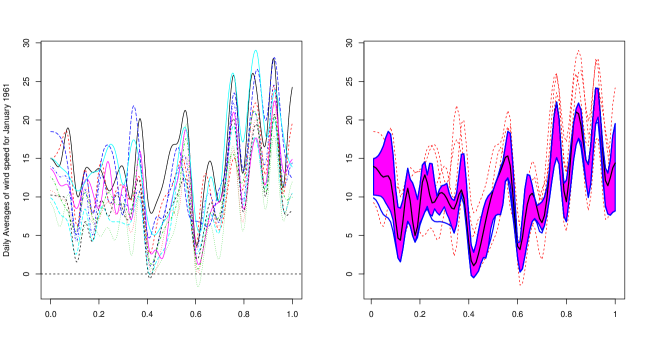
Figure 1: Irish wind speed curves for January 1961. Each is measured at a different location. The left panel plots the functional observations while the right gives a functional boxplot.

[2002] estimated model (4.1) on these data and obtained $\hat{\beta}=0.61$, which indicates a nonseparable covariance structure. We applied our tests to validate this conjecture. All four tests produced P–values smaller than 10E-4 for all $L,J\in\{2,3,4\}$. The P–values of the $T_{L}$–test were all smaller than 10E-104 and of the $T_{W}$–test smaller than 10E-21. The $T_{F}$–test had the largest P–values (but still extremely small).

While the tests fully validate the conclusion of [2002], we provide another illustration by applying them to residual curves obtained after removing the monthly mean from each curve; we center all January months, February months, etc., separately. This simple transformation removes to a large extent the annual seasonality, and it is interesting to see if a nonseparable structure is still needed for the data so transformed. The P–values for selected combinations of $L$ and $J$ are shown in Table 1. We now see a much more interesting pattern. Only when $L$ and $J$ are larger than $3$, do we see a clear evidence for nonseparability. A possible explanation is that the covariance structure is made up of two components, one which is separable and one which is not. The separable component makes up the majority of the variation in the process which is why the separability is not seen for smaller values of $L$ and $J$. The pattern of dependence of the P–values on $L$ and $J$ is inconsistent with what we have seen in Scenario 3 above, but this may be due to the specific parameter values in (4.1) we used in the simulations.

	$T_{L-MC}$	$T_{L}$	$T_{F}$	$T_{W}$
$L=J=2$	0.06	0.055	0.039	0.034
$L=J=3$	0.467	0.436	0.149	0.203
$L=J=4$	$<$10E-6	8.079E-24	4.237E-09	2.146E-09

Table 1: P–values for the separability tests applied to deseasonalized wind speed data.

Appendix A Derivation of the Q matrices

This section introduces four matrices that describe the covariance structure of products of various vectorized matrices consisting of standard normal variables. We refer to them collectively as “Q matrices”, as we use the symbol ${\bf Q}$ with suitable subscripts and superscripts to denote them. These matrices appear in the asymptotic distribution of the vectorized matrices $\widehat{\bf U},\widehat{\bf V},\widehat{\boldsymbol{\Sigma}}$, which, in turn, is used to prove Theorem 2.2. In particular, the asymptotic distribution of statistic $\widehat{T}_{F}$, which we recommended in Section 4, is expressed in terms of these Q matrices. Some of them are defined though an algorithm.

Theorem A.1.

If ${\bf E}$ is an $K\times I$ matrix of standard normals, then

(A.1) $$\operatorname{Cov}(\operatorname{vec}({\bf E}{\bf E}^{\top}))=2I{\bf Q}_{K}.$$

where

$${\bf Q}_{K}(i,j)=\begin{cases}1&i=j=k+(k-1)K\mbox{ for }k=1,\dots,K\\ \frac{1}{2}&i=j\neq k+(k-1)K\mbox{ for }k=1,\dots,K\\ \frac{1}{2}&i\neq j=1+\left(\frac{(i-1)-((i-1)\mbox{ mod }K)}{K}\right)+((i-1)\mbox{ mod }K)K\\ 0&\mbox{otherwise},\end{cases}.$$

Proof.

Denote by $e_{kl}$ the independent standard normals, and set

$${{\bf e}}_{k}=[e_{k1},e_{k2},\ldots,e_{kI}]^{\top},\ \ \ 1\leq k\leq K,$$

so that

$${\bf E}=\left[\begin{matrix}{\bf e}_{1}^{\top}\\ \vdots\\ {\bf e}_{K}^{\top}\end{matrix}\right].$$

Then for any $i,j$ in $\{1,\dots,K\}$ we have that the $(i,j)$ entry of $\operatorname{Cov}(\operatorname{vec}({\bf E}{\bf E}^{\top}))$ can be written as

$$\operatorname{Cov}({\bf e}_{k_{1}}^{\top}{\bf e}_{l_{1}},{\bf e}_{k_{2}}^{\top}{\bf e}_{l_{2}}),$$

where we have the relationships

$$i=k_{1}+(l_{1}-1)K,\qquad k_{1}=((i-1)\mbox{ mod }K)+1,\qquad l_{1}=1+\frac{(i-1)-(i-1)\mbox{ mod }K}{K}$$

$$j=k_{2}+(l_{2}-1)K,\qquad k_{2}=((j-1)\mbox{ mod }K)+1,\qquad l_{2}=1+\frac{(j-1)-(j-1)\mbox{ mod }K}{K}.$$

For the diagonal terms, i.e. $i=j$, we have two settings $k_{1}=k_{2}=l_{1}=l_{2}$, in which case the covariance is $2I$, or alternatively $k_{1}=k_{2}\neq l_{1}=l_{2}$ in which case the covariance is $I$. Since the former occurs in every $K^{th}$ term, we have established the proper pattern for the diagonal.

We now need only establish the pattern for the off diagonal. Every term in the off diagonal can be expressed as $\operatorname{Cov}({\bf e}_{i}^{\top}{\bf e}_{j},{\bf e}_{k}^{\top}{\bf e}_{l})$, for some $i,j,k,l=1,\dots,K$. Clearly, if any one index is different from the other 3, then the covariance is 0. We can’t have all four indices being equal as that would be a diagonal element, and we can’t have $i=k\neq j=k$ as that would also be a diagonal element. If $i=j$ and $k=l$ then two inner products are independent, and thus the covariance is zero. Therefore, the only nonzero off diagonal entries occur when $i=l\neq j=k$, and the covariance would be $I$. To determine where in the $K^{2}\times K^{2}$ matrix these occur, we use the change of base formulas. ∎

We illustrate the form of the matrices ${\bf Q}_{K}$:

$${\bf Q}_{2}=\left(\begin{matrix}1.0&0&0&0\\ 0&0.5&0.5&0\\ 0&0.5&0.5&0\\ 0&0&0&1.0\end{matrix}\right),$$

$${\bf Q}_{3}=\left(\begin{matrix}1.0&0&0&0&0&0&0&0&0\\ 0&0.5&0&0.5&0&0&0&0&0\\ 0&0&0.5&0&0&0&0.5&0&0\\ 0&0.5&0&0.5&0&0&0&0&0\\ 0&0&0&0&1.0&0&0&0&0\\ 0&0&0&0&0&0.5&0&0.5&0\\ 0&0&0.5&0&0&0&0.5&0&0\\ 0&0&0&0&0&0.5&0&0.5&0\\ 0&0&0&0&0&0&0&0&1.0\end{matrix}\right).$$

Theorem A.2.

If ${\bf E}$ is an $K\times I$ matrix of standard normals, then

(A.2) $$\operatorname{Cov}(\operatorname{vec}({\bf E}{\bf E}^{\top}),\operatorname{vec}({\bf E}^{\top}{\bf E}))=2\sqrt{IK}{\bf Q}_{K,I},$$

where ${\bf Q}_{K,I}$ is an $K^{2}\times I^{2}$ matrix given by

$${\bf Q}_{K,I}(i,j)=\begin{cases}(KI)^{-1/2}&i=k_{1}+K(k_{1}-1),j=k_{2}+I(k_{2}-1)\ k_{1}=1,\dots,K\ k_{2}=1,\dots,I\\ 0&\mbox{otherwise},\end{cases}.$$

Proof.

Here, each entry of the above covariance matrix is obtained by taking two rows of ${\bf E}$ (possibly the same row) forming the inner product, taking two columns, taking their inner product, and then computing the covariance between the two. Due to the symmetry of this calculation, there are only three possible resulting values: when the two rows are different, then the two columns are different, or when both the rows and columns are different. When both rows and columns are different, we can (without loss of generality) take the first two rows and columns. In that case, the covariance becomes

$$\operatorname{Cov}\left(\sum_{k=1}^{K}e_{1,k}e_{2,k},\sum_{i=1}^{I}e_{i,1}e_{i,2}\right)=\sum_{k=1}^{K}\sum_{i=1}^{I}\operatorname{Cov}\left(e_{1,k}e_{2,k},e_{i,1}e_{i,2}\right).$$

However, every summand above is zero when $i>2$ or $k>2$ since they will then involve independent variables. Therefore, we can express the above as

$$\operatorname{Cov}(e_{1,1}e_{2,1}+e_{1,2}e_{2,2},e_{1,1}e_{1,2}+e_{2,1}e_{2,2})=0.$$

Hence, any term with two different rows and columns is zero. A similar result will hold when there are either two different rows or two different columns. The only nonzero term will stem from taking the same row and same column, in which case the value becomes

$$\operatorname{Cov}(e_{1,1}e_{1,1}+e_{1,2}e_{1,2},e_{1,1}e_{1,1}+e_{2,1}e_{2,1})=\operatorname{Var}(e_{1,1}^{2})=2.$$

Therefore, every nonzero entry will be 2. We now only need to determine which entries of the covariance matrix correpond to taking the same row and same column. Considering the structure induced by vectorizing, the first row of the covariance matrix and every subsequent $K$ rows will correspond to matching the same row of ${\bf E}$. Similalry, the first and every subsequent $I$ column will correspond to matching the same colmun of ${\bf E}$. This corresponds to our definition and the result follows.

∎

Some examples ${\bf Q}_{K,I}$ are

$${\bf Q}_{2,2}=\left(\begin{matrix}0.5&0&0&0.5\\ 0&0&0&0\\ 0&0&0&0\\ 0.5&0&0&0.5\end{matrix}\right)$$

and

$${\bf Q}_{2,3}=\left(\begin{matrix}6^{-1/2}&0&0&0&6^{-1/2}&0&0&0&6^{-1/2}\\ 0&0&0&0&0&0&0&0&0\\ 0&0&0&0&0&0&0&0&0\\ 6^{-1/2}&0&0&0&6^{-1/2}&0&0&0&6^{-1/2}\\ \end{matrix}\right).$$

Before the next theorem, we define the matrix $\tilde{\bf Q}_{R,K}$ via a pseudo code.

Begin Code

Set $\tilde{\bf Q}_{R,K}$ to be an $R^{2}=K^{2}I^{2}$ by $K^{2}$ matrix of zeros

For $i=1,\dots,R^{2}$

$l=1+\lfloor(i-1)/(K^{2}I)\rfloor$

$k=1+\lfloor(i-1-(l-1)K^{2}T)/(KI)\rfloor$

$p=1+\lfloor(i-1-(l-1)K^{2}I-(k-1)KI)/(K)\rfloor$

$m=i-(l-1)K^{2}I-(k-1)KI-(p-1)K$

If ($p=l$ and $m\neq k$) then $\tilde{\bf Q}_{R,K}[i,m+(k-1)K]=1/(2\sqrt{I})$

and $\tilde{\bf Q}_{R,K}[i,k+(m-1)K]=1/(2\sqrt{I})$

If ($p=l$ and $m=k$) then $\tilde{\bf Q}_{R,K}[i,m+(m-1)K]=1/\sqrt{I}$

End For Loop

End Code

Theorem A.3.

If ${\bf E}$ is an $K\times I$ matrix of standard normals and ${\bf E}_{\diamond}=\operatorname{vec}({\bf E})$, then

(A.3) $$\operatorname{Cov}(\operatorname{vec}({\bf E}_{\diamond}{\bf E}_{\diamond}^{\top}),\operatorname{vec}({\bf E}{\bf E}^{\top}))=2\sqrt{T}\tilde{\bf Q}_{R,K},$$

where $\tilde{\bf Q}_{R,K}$ is the $R^{2}\times K^{2}$ matrix defined by the pseudo code above.

Proof.

Begin by considering the $(i,j)$ of the desired covariance matrix. There exists indices such that the $(i,j)$ entry is equal to

$$\operatorname{Cov}(e_{m,p}e_{k,l},e_{r}^{\top}e_{s}),$$

where $m,k,r,s$ take values $1,\dots,K$ and $p,l$ take values $1,\dots,I$. Moving from $(r,s)$ to $j$ we have that

$$j=1+(r-1)+(s-1)K,$$

and the reverse is obtained using

$$s =1+\lfloor(j-1)/K\rfloor$$

$$r =j-(s-1)K.$$

Moving from $(m,p,k,l)$ to $i$ we have that

$$i=1+(m-1)+(p-1)K+(k-1)KI+(l-1)K^{2}I.$$

We can move back to $(m,p,k,l)$ from $i$ using

$$l =1+\lfloor(i-1)/(K^{2}I)\rfloor$$

$$k =1+\lfloor(i-1-(l-1)K^{2}I)/(KI)\rfloor$$

$$p =1+\lfloor(i-1-(l-1)K^{2}I-(k-1)KI)/(K)\rfloor$$

$$m =i-(l-1)K^{2}I-(k-1)KI-(p-1)K.$$

We can see that the covariance will be zero if any one of $m,k,r$ or $s$ is distinct. Thus, the only nonzero entries will correspond to either $m=r=k=s$, $m=r\neq k=s$, or $m=s\neq k=r$ (when $m=k\neq r=s$ we get zero). When all four are equal we get that

$$\operatorname{Cov}(e_{m,p}e_{m,l},e_{m}^{\top}e_{m})=\operatorname{Cov}(e_{m,p}e_{m,l},e_{m,p}^{2}+e_{m,l}^{2}1_{p\neq l}),$$

which will be zero unless $p=l$, in which case it equals

$$\operatorname{Cov}(e_{m,p}^{2},e_{m,p}^{2})=(\operatorname{E}[e_{m,p}^{4}]-\operatorname{E}[e_{m,p}^{2}]^{2})=2.$$

We have therefore established the first if-statement in the pseudo code.

Turning to the next case, when $m=r\neq k=s$, we have that

$$\operatorname{Cov}(e_{m,p}e_{k,l},e_{m}^{\top}e_{k})=\operatorname{Cov}(e_{m,p}e_{k,l},e_{m,p}e_{k,p}+e_{m,l}e_{k,l}1_{l\neq p}),$$

which is again only nonzero when $p=l$, in which case it will be

$$\operatorname{Cov}(e_{m,p}e_{k,p},e_{m,p}e_{k,p})=\operatorname{E}[e_{m,p}^{2}]\operatorname{E}[e_{k,p}^{2}]=1.$$

An identical result will hold for when $m=s\neq k=r$, which gives both the second and third if-statements in the pseudo code, and the proof is established. ∎

One example of $\tilde{\bf Q}_{R,K}$ is

$$\tilde{\bf Q}_{4,2}=\left(\begin{matrix}2^{-1/2}&0&0&0\\ 0&8^{-1/2}&8^{-1/2}&0\\ 0&0&0&0\\ 0&0&0&0\\ 0&8^{-1/2}&8^{-1/2}&0\\ 0&0&0&2^{-1/2}\\ 0&0&0&0\\ 0&0&0&0\\ 0&0&0&0\\ 0&0&0&0\\ 2^{-1/2}&0&0&0\\ 0&8^{-1/2}&8^{-1/2}&0\\ 0&0&0&0\\ 0&0&0&0\\ 0&8^{-1/2}&8^{-1/2}&0\\ 0&0&0&2^{-1/2}\end{matrix}\right).$$

For the last Q matrix, we also use pseudo code which is only slightly different from the code defining $\tilde{\bf Q}_{R,K}$.

Begin Code

Set $\breve{\bf Q}_{R,I}$ to be an $R^{2}=K^{2}I^{2}$ by $I^{2}$ matrix of zeros

For $i=1,\dots,R^{2}$

$l=1+\lfloor(i-1)/(K^{2}I)\rfloor$

$k=1+\lfloor(i-1-(l-1)K^{2}I)/(KI)\rfloor$

$p=1+\lfloor(i-1-(l-1)K^{2}I-(k-1)KI)/(K)\rfloor$

$m=i-(l-1)K^{2}I-(k-1)KI-(p-1)K$

If ($m=k$ and $p\neq l$) then $\breve{\bf Q}_{R,I}[i,p+(l-1)I]=1/(2\sqrt{K})$

and $\breve{\bf Q}_{R,I}[i,l+(p-1)I]=1/(2\sqrt{K})$

If ($m=k$ and $p=l$) then $\breve{\bf Q}_{R,I}[i,l+(l-1)I]=1/\sqrt{K}$

End For Loop

End Code

Theorem A.4.

If ${\bf E}$ is an $K\times I$ matrix of standard normals and ${\bf E}_{\diamond}=\operatorname{vec}({\bf E})$, then

(A.4) $$\operatorname{Cov}(\operatorname{vec}({\bf E}_{\diamond}{\bf E}_{\diamond}^{\top}),\operatorname{vec}({\bf E}^{\top}{\bf E}))=2\sqrt{K}\breve{\bf Q}_{R,I},$$

where $\breve{\bf Q}_{R,I}$ is the $R^{2}\times I^{2}$ matrix defined by the pseudo code above.

Proof.

Begin by considering the $(i,j)$ of the desired covariance matrix. There exists indices such that the $(i,j)$ entry is equal to

$$\operatorname{Cov}(e_{m,p}e_{k,l},e_{(r)}^{\top}e_{(s)}),$$

where $m,k$ take values $1,\dots,K$ and $p,l,r,s$ take values $1,\dots,I$. Moving from $(r,s)$ to $j$ we have that

$$j=1+(r-1)+(s-1)I,$$

and the reverse is obtained using

$$s =1+\lfloor(j-1)/I\rfloor$$

$$r =j-(s-1)I.$$

Moving from $(m,p,k,l)$ to $i$ we have that

$$i=1+(m-1)+(p-1)K+(k-1)KI+(l-1)K^{2}I.$$

We can move back to $(m,p,k,l)$ from $i$ using

$$l =1+\lfloor(i-1)/(K^{2}I)\rfloor$$

$$k =1+\lfloor(i-1-(l-1)K^{2}I)/(KI)\rfloor$$

$$p =1+\lfloor(i-1-(l-1)K^{2}I-(k-1)KI)/(K)\rfloor$$

$$m =i-(l-1)I^{2}K-(k-1)KI-(p-1)K.$$

We can see that the covariance will be zero if any one of $p,l,r$ or $s$ is distinct. Thus, the only nonzero entries will correspond to either $p=r=l=s$, $p=r\neq l=s$, or $p=s\neq l=r$ (when $p=l\neq r=s$ we get zero). When all four are equal we get that

$$\operatorname{Cov}(e_{m,p}e_{k,p},e_{(p)}^{\top}e_{(p)})=\operatorname{Cov}(e_{m,p}e_{k,p},e_{m,p}^{2}+e_{k,p}^{2}1_{m\neq k}),$$

which will be zero unless $m=k$, in which case it equals it will be equal to 2. We have therefore established the first if-statement in the pseudo code.

Turning to the next case, when $p=r\neq l=s$, we have that

$$\operatorname{Cov}(e_{m,p}e_{k,l},e_{(p)}^{\top}e_{(l)})=\operatorname{Cov}(e_{m,p}e_{k,l},e_{m,p}e_{m,l}+e_{k,p}e_{k,l}1_{m\neq k}),$$

which is again only nonzero when $m=k$, in which case it will be

$$\operatorname{Cov}(e_{m,p}e_{m,l},e_{m,p}e_{m,l})=\operatorname{E}[e_{m,p}^{2}]\operatorname{E}[e_{m,l}^{2}]=1.$$

An identical result will hold for when $p=s\neq l=r$, which gives both the second and third if-statements in the pseudo code, and the proof is established. ∎

Appendix B Proof of Theorem 2.2

We begin by establishing in Theorem B.1 the joint null limit distribution of the vectors $\operatorname{vec}(\hat{\bf U}-{\bf U}),\operatorname{vec}(\hat{\bf V}-{\bf V})$, and $\operatorname{vec}(\hat{\boldsymbol{\Sigma}}-{\boldsymbol{\Sigma}})$. We first define several matrices that appear in this distribution. Recall the Q matrices derived in Section A: the matrix ${\bf Q}_{K}$ is defined in (A.1), ${\bf Q}_{K,I}$ in (A.2), $\tilde{\bf Q}_{R,K}$ in (A.3), and $\breve{\bf Q}_{R,I}$ in (A.4). Denote by $(\cdot)^{+}$ a generalized inverse. We define the following generalized information matrices:

$${\mathcal{I}}_{{\bf U},{\bf V}}= \frac{1}{2}\left(\begin{matrix}{\bf U}^{-1/2}\otimes{\bf U}^{-1/2}&0\\ 0&{\bf V}^{-1/2}\otimes{\bf V}^{-1/2}\end{matrix}\right)$$

$$\times\left(\begin{matrix}I{\bf Q}_{K}&\sqrt{IK}{\bf Q}_{K,I}\\ \sqrt{IK}{\bf Q}_{I,K}&K{\bf Q}_{I}\end{matrix}\right)\left(\begin{matrix}{\bf U}^{-1/2}\otimes{\bf U}^{-1/2}&0\\ 0&{\bf V}^{-1/2}\otimes{\bf V}^{-1/2}\end{matrix}\right),$$

$${\mathcal{I}}_{{\bf U},{\bf V}}^{c}= ({\bf D}({\bf D}^{\top}{\mathcal{I}}_{{\bf U},{\bf V}}{\bf D})^{+}{\bf D}^{\top})^{+},$$

where ${\bf D}$ is an $(K^{2}+I^{2})\times(K^{2}+I^{2}-1)$ matrix whose columns are orthonormal and are perpendicular to $\operatorname{vec}({\bf I}_{K^{2}+I^{2}})$, and

$${\mathcal{I}}_{{\boldsymbol{\Sigma}}}=\frac{1}{2}({\boldsymbol{\Sigma}}^{-1/2}\otimes{\boldsymbol{\Sigma}}^{-1/2}){\bf Q}_{R}({\boldsymbol{\Sigma}}^{-1/2}\otimes{\boldsymbol{\Sigma}}^{-1/2}),$$

where $R=KI$.

Theorem B.1.

Suppose Assumption 2.1 and decomposition (2.1) hold. Assume further that $\operatorname{tr}({\bf U})=K$. Then

$$\sqrt{N}\left(\begin{matrix}\operatorname{vec}(\hat{\bf U}-{\bf U})\\ \operatorname{vec}(\hat{\bf V}-{\bf V})\\ \operatorname{vec}(\hat{\boldsymbol{\Sigma}}-{\boldsymbol{\Sigma}})\end{matrix}\right)\overset{{\mathcal{D}}}{\to}N({\bf 0},\mbox{\boldmath${\Gamma}$}).$$

The asymptotic covariance matrix ${\Gamma}$ is defined as follows. The asymptotic covariance of $(\operatorname{vec}(\hat{\bf U}-{\bf U}),\operatorname{vec}(\hat{\bf V}-{\bf V}))$ is given by $({\mathcal{I}}_{{\bf U},{\bf V}}^{c})^{+}$, of $\operatorname{vec}(\hat{\boldsymbol{\Sigma}}-{\boldsymbol{\Sigma}})$ is given by ${\mathcal{I}}_{{\boldsymbol{\Sigma}}}^{+}$, and the cross covariance matrix between the two is

$$\frac{1}{2}({\mathcal{I}}^{c}_{{\bf U},{\bf V}})^{+}\left(\begin{matrix}{\bf U}^{-1/2}\otimes{\bf U}^{-1/2}&0\\ 0&{\bf V}^{-1/2}\otimes{\bf V}^{-1/2}\end{matrix}\right)\left(\begin{matrix}\sqrt{I}\tilde{\bf Q}_{R,K}^{\top}\\ \sqrt{K}\breve{\bf Q}_{R,I}^{\top}\end{matrix}\right)({\boldsymbol{\Sigma}}^{-1/2}\otimes{\boldsymbol{\Sigma}}^{-1/2}){\mathcal{I}}^{+}_{{\boldsymbol{\Sigma}}}.$$

Proof.

From standard theory for MLEs, [1996] Chapter 18, we can use the partial derivatives of the log likelihood function (score equations) to find the Fisher information as well as asymptotic expressions for the MLEs. One can show that the cross terms of the Fisher information involving ${\bf M}$ and ${\bf V},{\bf U}$ and ${\boldsymbol{\Sigma}}$ are all zero, meaning that the estimate of the ${\bf M}$ is asymptotically independent of $\widehat{\bf U},\widehat{\bf V}$ and $\widehat{\boldsymbol{\Sigma}}$. We therefore treat in the following ${\bf M}$ as known.

We start by working with ${\bf U}$ and ${\bf V}$. Applying the constrained likelihood methods described in [2008], asymptotically, $\widehat{\bf U}$ and $\widehat{\bf V}$ are jointly normally distributed with means ${\bf U}$ and ${\bf V}$ and covariance given by the generalized inverse of the constrained Fisher information matrix. Starting with ${\bf U}$ we have that unconstrained score equation is given by

$$\frac{1}{\sqrt{N}}\frac{\partial l({\bf M},{\bf U},{\bf V})}{\partial{\bf U}}$$

$$=\frac{1}{2\sqrt{N}}\sum_{n=1}^{N}[{\bf U}^{-1}({\bf X}_{n}-{\bf M}){\bf V}^{-1}({\bf X}_{n}-{\bf M})^{\top}{\bf U}^{-1}-T{\bf U}^{-1}]$$

$$=\frac{1}{2\sqrt{N}}\sum_{n=1}^{N}[{\bf U}^{-1/2}{\bf E}_{n}{\bf E}_{n}^{\top}{\bf U}^{-1/2}-T{\bf U}^{-1}]$$

$$=\frac{1}{2\sqrt{N}}\sum_{n=1}^{N}[{\bf U}^{-1/2}[{\bf E}_{n}{\bf E}_{n}^{\top}-I{\bf I}_{K\times K}]{\bf U}^{-1/2}].$$

To get a handle on the unconstrained Fisher information matrix (and therefore the covariance matrix), it will be easier to work with the vectorized version

$$\frac{1}{2\sqrt{N}}({\bf U}^{-1/2}\otimes{\bf U}^{-1/2})\sum_{n=1}^{N}\operatorname{vec}[{\bf E}_{n}{\bf E}_{n}^{\top}-I{\bf I}_{K\times K}].$$

Notice that we will have a complete handle on the above if we can understand the form for the covariance of $\operatorname{vec}[{\bf E}_{n}{\bf E}_{n}^{\top}-I{\bf I}_{K\times K}]$. However, this is a term that in no way depends on the underlying parameters as it is composed entirely of iid standard normals. We label ${\bf Q}_{K}=(2I)^{-1}\operatorname{Cov}(\operatorname{vec}[{\bf E}_{n}{\bf E}_{n}^{\top}-I{\bf I}_{K\times K}])$ and its explicit form is given in (A.1).

The part of the Fisher information matrix for $\operatorname{vec}({\bf U})$ is given by

$$\frac{I}{2}({\bf U}^{-1/2}\otimes{\bf U}^{-1/2}){\bf Q}_{K}({\bf U}^{-1/2}\otimes{\bf U}^{-1/2}).$$

Identical arguments give that the part of the Fisher information matrix for $\operatorname{vec}({\bf V})$ is given by

$$\frac{K}{2}({\bf V}^{-1/2}\otimes{\bf V}^{-1/2}){\bf Q}_{I}({\bf V}^{-1/2}\otimes{\bf V}^{-1/2}).$$

The joint unconstrained Fisher information matrix for $\widehat{\bf U}$ and $\widehat{\bf V}$ is given by

$${\mathcal{I}}_{{\bf U},{\bf V}}=\frac{1}{2} \left(\begin{matrix}{\bf U}^{-1/2}\otimes{\bf U}^{-1/2}&0\\ 0&{\bf V}^{-1/2}\otimes{\bf V}^{-1/2}\end{matrix}\right)$$

$$\times\left(\begin{matrix}I{\bf Q}_{K}&\sqrt{IK}{\bf Q}_{I,K}\\ \sqrt{IK}{\bf Q}_{I,K}&K{\bf Q}_{I}\end{matrix}\right)\left(\begin{matrix}{\bf U}^{-1/2}\otimes{\bf U}^{-1/2}&0\\ 0&{\bf V}^{-1/2}\otimes{\bf V}^{-1/2}\end{matrix}\right),$$

where ${\bf Q}_{K,I}$ is defined in (A.2). The constrained version is then given by

$${\mathcal{I}}_{{\bf U},{\bf V}}^{c}=({\bf D}({\bf D}^{\top}{\mathcal{I}}_{{\bf U},{\bf V}}{\bf D}){\bf D}^{+})^{+}.$$

Recall that ${\bf D}$ is an $(K^{2}+I^{2})\times(K^{2}+I^{2}-1)$ matrix whose columns are orthonormal and are perpendicular to $\operatorname{vec}({\bf I}_{K^{2}+I^{2}})$. The form for ${\bf D}$ come from the gradient of the constraint $\operatorname{tr}({\bf U})=K$.

The last piece we need is the joint behavior of $\widehat{\bf U}$ (or $\widehat{\bf V}$) and the estimator $\widehat{\boldsymbol{\Sigma}}$. The score equation for ${\boldsymbol{\Sigma}}$ can be expressed as

$$\frac{\partial l(\mu,{\boldsymbol{\Sigma}})}{\partial{\boldsymbol{\Sigma}}} =-\frac{N}{2}{\boldsymbol{\Sigma}}^{-1}+\frac{1}{2}{\boldsymbol{\Sigma}}^{-1}\left(\sum_{n=1}^{N}(Y_{n}-\mu)(Y_{n}-\mu)\right){\boldsymbol{\Sigma}}^{-1}$$

$$=-\frac{N}{2}{\boldsymbol{\Sigma}}^{-1}+\frac{1}{2}{\boldsymbol{\Sigma}}^{-1/2}\left(\sum_{n=1}^{N}E_{n}E_{n}^{\top}\right){\boldsymbol{\Sigma}}^{-1/2}$$

$$=\frac{1}{2}{\boldsymbol{\Sigma}}^{-1/2}\left(\sum_{n=1}^{N}E_{n}E_{n}^{\top}-{\bf I}_{KI\times KI}\right){\boldsymbol{\Sigma}}^{-1/2}.$$

Using the same arguments as before, we get that Fisher information matrix for $\operatorname{vec}({\boldsymbol{\Sigma}})$ is

$${\mathcal{I}}_{\boldsymbol{\Sigma}}=\frac{1}{2}({\boldsymbol{\Sigma}}^{-1/2}\otimes{\boldsymbol{\Sigma}}^{-1/2}){\bf Q}_{R}({\boldsymbol{\Sigma}}^{-1/2}\otimes{\boldsymbol{\Sigma}}^{-1/2}).$$

For the joint behavior, we use the following asymptotic expression for the MLEs, [1996] Chapter 18,

$$\sqrt{N}\left(\begin{matrix}\operatorname{vec}(\widehat{\bf U}-{\bf U})\\ \operatorname{vec}(\widehat{\bf V}-{\bf V})\\ \end{matrix}\right)=\frac{1}{\sqrt{N}}({\mathcal{I}}^{c}_{{\bf U},{\bf V}})^{+}\left(\begin{matrix}\operatorname{vec}\left(\frac{\partial l({\bf M},{\bf U},{\bf V})}{\partial{\bf U}}\right)\\ \operatorname{vec}\left(\frac{\partial l({\bf M},{\bf U},{\bf V})}{\partial{\bf V}}\right)\\ \end{matrix}\right)+o_{P}(1),$$

and

$$\sqrt{N}\operatorname{vec}(\widehat{\boldsymbol{\Sigma}}-{\boldsymbol{\Sigma}})=\frac{1}{\sqrt{N}}{\mathcal{I}}^{+}_{{\boldsymbol{\Sigma}}}\frac{\partial l(\mu,{\boldsymbol{\Sigma}})}{\partial{\boldsymbol{\Sigma}}}+o_{P}(1).$$

For the covariance between $\widehat{\boldsymbol{\Sigma}}$ and $\widehat{\bf U}$ (or $\widehat{\bf V}$) we obtain two more matrices, called $\tilde{\bf Q}_{R,K}$ and $\breve{\bf Q}_{R,I}$ which satisfy

$$\operatorname{Cov}\left[\operatorname{vec}({\bf E}_{\diamond n}{\bf E}_{\diamond n}^{\top}-{\bf I}_{R\times R}),\operatorname{vec}({\bf E}_{n}{\bf E}_{n}^{\top}-I{\bf I}_{K\times K})\right]=2\sqrt{I}\tilde{\bf Q}_{R,K},$$

$$\operatorname{Cov}\left[\operatorname{vec}({\bf E}_{\diamond n}{\bf E}_{\diamond n}^{\top}-{\bf I}_{R\times R}),\operatorname{vec}({\bf E}_{n}^{\top}{\bf E}_{n}-K{\bf I}_{I\times I})\right]=2\sqrt{K}\breve{\bf Q}_{R,I}.$$

Recall that the diamond subscript indicates vectorization and the definitions of $\tilde{\bf Q}_{R,K}$ and $\breve{\bf Q}_{R,I}$ can be found in (A.3) and (A.4), respectively. The cross–covariance matrix for $\sqrt{N}\operatorname{vec}(\widehat{\boldsymbol{\Sigma}}-{\boldsymbol{\Sigma}})$ and $\sqrt{N}\operatorname{vec}(\widehat{\bf U}-{\bf U})$ is then given by

$$({\mathcal{I}}^{c}_{{\bf U},{\bf V}})^{+}\operatorname{Cov}\left(\left(\begin{matrix}\operatorname{vec}\left(N^{-1/2}\frac{\partial l(M,U,V)}{\partial U}\right)\\ \operatorname{vec}\left(N^{-1/2}\frac{\partial l(M,U,V)}{\partial V}\right)\\ \end{matrix}\right),\operatorname{vec}\left(N^{-1/2}\frac{\partial l(M,\Sigma)}{\partial\Sigma}\right)\right){\mathcal{I}}^{+}_{{\boldsymbol{\Sigma}}}$$

$$=\frac{1}{2}({\mathcal{I}}^{c}_{{\bf U},{\bf V}})^{+}\left(\begin{matrix}{\bf U}^{-1/2}\otimes{\bf U}^{-1/2}&0\\ 0&{\bf V}^{-1/2}\otimes{\bf V}^{-1/2}\end{matrix}\right)\left(\begin{matrix}\sqrt{I}\tilde{\bf Q}_{R,K}^{\top}\\ \sqrt{K}\breve{\bf Q}_{R,I}^{\top}\end{matrix}\right)({\boldsymbol{\Sigma}}^{-1/2}\otimes{\boldsymbol{\Sigma}}^{-1/2}){\mathcal{I}}^{+}_{{\boldsymbol{\Sigma}}}$$

∎

Proof of Theorem 2.2: Since we have the joint asymptotic distribution for $\widehat{\bf U},\widehat{\bf V},$ and $\widehat{\boldsymbol{\Sigma}}$, we can use the delta method to find the asymptotic distributions of desired test statistics, and in particular, we can find the form of ${\bf W}$, the asymptotic covariance matrix of $\operatorname{vec}(\widehat{\bf V}\otimes\widehat{\bf U})-\operatorname{vec}(\widehat{\boldsymbol{\Sigma}}).$ To apply the delta method, we need the partial derivatives. Taking the derivative with respect to $V_{i,j}$ yields

$$\operatorname{vec}(\mbox{\boldmath${1}$}_{i,j}\otimes{\bf U})$$

and with respect to $U_{k,l}$

$$\operatorname{vec}({\bf V}\otimes\mbox{\boldmath${1}$}_{k,l}).$$

So the matrix of partials with respect to $\operatorname{vec}({\bf V})$ is

$${\bf G}_{\bf V}=\left(\begin{matrix}\operatorname{vec}(\mbox{\boldmath${1}$}_{1,1}\otimes{\bf U})^{\top}\\ \operatorname{vec}(\mbox{\boldmath${1}$}_{2,1}\otimes{\bf U})^{\top}\\ \vdots\\ \operatorname{vec}(\mbox{\boldmath${1}$}_{I,I}\otimes{\bf U})^{\top}\end{matrix}\right),$$

with respect to $\operatorname{vec}({\bf U})$ is

$${\bf G}_{\bf U}=\left(\begin{matrix}\operatorname{vec}({\bf V}\otimes\mbox{\boldmath${1}$}_{1,1})^{\top}\\ \operatorname{vec}({\bf V}\otimes\mbox{\boldmath${1}$}_{2,1})^{\top}\\ \vdots&\\ \operatorname{vec}({\bf V}\otimes\mbox{\boldmath${1}$}_{K,K})^{\top}\end{matrix}\right),$$

and with respect to $\operatorname{vec}({\boldsymbol{\Sigma}})$ is just $(-1)$ times the $KI\times KI$ identity matrix. We therefore have that

$$\operatorname{vec}(\widehat{\bf V}\otimes\widehat{\bf U})-\operatorname{vec}(\widehat{\boldsymbol{\Sigma}})\approx\left(\begin{matrix}{\bf G}_{\widehat{\bf U}}\\ {\bf G}_{\widehat{\bf V}}\\ -{\bf I}_{ST\times ST}\end{matrix}\right)^{\top}\left(\begin{matrix}\operatorname{vec}(\widehat{\bf U})\\ \operatorname{vec}(\widehat{\bf V})\\ \operatorname{vec}(\widehat{\boldsymbol{\Sigma}})\end{matrix}\right).$$

This implies that

(B.1) $${\bf W}=\left(\begin{matrix}{\bf G}_{{\bf U}}\\ {\bf G}_{{\bf V}}\\ -{\bf I}_{KI\times KI}\end{matrix}\right)^{\top}\mbox{\boldmath${\Gamma}$}\left(\begin{matrix}{\bf G}_{{\bf U}}\\ {\bf G}_{{\bf V}}\\ -{\bf I}_{KI\times KI}\end{matrix}\right).$$

The degrees of freedom are obtained by noticing that under the alternative ${\boldsymbol{\Sigma}}$ has $KI(KI+1)/2$ free parameters, while under the null there $K(K+1)/2+I(I+1)/2-1$, where the last $-1$ is included because we have one constraint ($\operatorname{tr}({\bf U})=K$).

References

Aston et al. (2015)
Aston, J. A. D., Pigoli, D. and Tavakoli, S.
(?).
Tests for separability in nonparametric covariance operators of
random surfaces.
Technical report. University of Cambridge, Cambridge, UK.
2010
Delicado, P., Giraldo, R., Comas, C. and Mateu, J.
(?).
Statistics for spatial functional data: some recent contributions.
Environmetrics, 21, 224–239.
1999
Dutilleul, P.
(?).
The MLE algorithm for the matrix normal distribution.
Journal of Statistical Computing and Simulation, 64, 105–123.
1996
Ferguson, T. S.
(?).
A Course in Large Sample Theory.
Chapman & Hall, London.
2006
Fuentes, M.
(?).
Testing for separability of spatial–temporal covariance functions.
Journal of Multivariate Analysis, 136, 447–466.
2007
Genton, M. G.
(?).
Separable approximations of space-time covariance matrices.
Environmetrics, 18, 681–695.
2002
Gneiting, T.
(?).
Nonseparable, stationary covariance functions for space–time data.
Journal of the American Statistical Association, 97, 590–600.
2012
Gromenko, O. and Kokoszka, P.
(?).
Testing the equality of mean functions of spatially distributed
curves.
Journal of the Royal Statistical Society (C), 61,
715–731.
2013
Gromenko, O. and Kokoszka, P.
(?).
Nonparametric inference in small data sets of spatially indexed
curves with application to ionospheric trend determination.
Computational Statistics and Data Analysis, 59,
82–94.
2015
Gromenko, O., Kokoszka, P. and Reimherr, M.
(?).
Detection of change in the spatio–temporal mean function.
Journal of the Royal Statistical Society (B), 00,
000–000; under minor revision.
2012
Gromenko, O., Kokoszka, P., Zhu, L. and Sojka, J.
(?).
Estimation and testing for spatially indexed curves with application
to ionospheric and magnetic field trends.
The Annals of Applied Statistics, 6, 669–696.
1995
Haas, T. C.
(?).
Local Prediction of a Spatio-Temporal Process with an
Application to Wet Sulfate Deposition.
Journal of the American Statistical Association, 90, 1189–1199.
1989
Haslett, J. and Raftery, A. E.
(?).
Space–time modelling with long–memory dependence: assesing
Ireland’s wind power resource.
Appl. Statist., 38, number 1, 1–50.
2011
Hoff, P. D.
(?).
Separable covariance arrays via the tucker product, with applications
to multivariate relational data.
Bayesian Analysis, 6, 179–196.
2012
Horváth, L. and Kokoszka, P.
(?).
Inference for Functional Data with Applications.
Springer.
2015
Hsing, Tailen and Eubank, Randall
(?).
Theoretical foundations of functional data analysis, with an
introduction to linear operators.
John Wiley & Sons.
2014
Liu, C., Ray, S. and Hooker, G.
(?).
Functional principal components analysis of spatially correlated
data.
Technical report. University of Glasgow.
Available at http://arxiv.org/abs/1411.4681.
2005
Lu, N. and Zimmerman, D.
(?).
The likelihood ratio test for a separable covariance matrix.
Statistics & Probability Letters, 73, 449–457.
2005
Mitchell, M. W., Genton, M. G. and Gumpertz, M. L.
(?).
Testing for separability of space–time covariances.
Environmetrics, 16, 819–831.
2006
Mitchell, M. W., Genton, M. G. and Gumpertz, M. L.
(?).
A likelihood ratio test for separability of covariances.
Journal of Multivariate Analysis, 97, 1025–1043.
2008
Moore, J. T., B. M. Sadler, Brian M and Kozick, R. J.
(?).
Maximum-likelihood estimation, the Cramér–Rao bound, and the
method of scoring with parameter constraints.
IEEE Transactions on Signal Processing, 56,
895–908.
2011
Paul, D. and Peng, J.
(?).
Principal components analysis for sparsely observed correlated
functional data using a kernel smoothing approach.
Electronic Journal of Statistics, 5, 1960–2003.
2009
Ramsay, J., Hooker, G. and Graves, S.
(?).
Functional Data Analysis with R and MATLAB.
Springer.
2005
Ramsay, J. O. and Silverman, B. W.
(?).
Functional Data Analysis.
Springer.
2005
Schabenberger, O. and Gotway, C. A.
(?).
Statistical Methods for Spatial Data Analysis.
Chapman & Hall/CRC.
2011
Sherman, M.
(?).
Spatial Statistics and Spatio–Temporal data: Covariance
Functions and Directional Properties.
Wiley.
2011
Sun, Y. and Genton, M. G.
(?).
Functional boxplots.
Journal of Computational and Graphical Statistics, 20, 316–334.
2012
Sun, Y., Li, B. and Genton, M.G.
(?).
Geostatistics for large datasets.
In Advances and Challenges in Space-time Modelling of
Natural Events, Berlin (eds E. Porcu, J.M. Montero and M.
Schlather), chapter 3, pp. 55–77.
Springer.