Frequency shifts and relaxation rates for spin-1/2 particles moving in electromagnetic fields

Abstract

We discuss the behavior of the Larmor frequency shift and the longitudinal relaxation rate due to non-uniform electromagnetic fields on an assembly of spin 1/2 particles, in adiabatic and nonadiabatic regimes. We also show some general relations between the various frequency shifts and between the frequency shifts and relaxation rates. The remarkable feature of all our results is that they are obtained without any specific assumptions on the explicit form of the correlation functions of the fields. Hence, we expect that our results are valid for both diffusive and ballistic regimes of motion and for arbitrary cell shapes and surface scattering. These results can then be applied to a wide variety of realistic systems.

I Introduction

The behavior of a system of spins interacting with static and time varying magnetic fields is a very broad topic and has been the subject of intense study for decades. A very important application is to the study of spins interacting with the randomly fluctuating fields associated with a thermal reservoir. Bloembergen, Purcell and Pound Bloembergen et al. (1948) have treated this problem using physical arguments based on Fermi’s golden rule and showed that the relaxation induced by the fields associated with a thermal reservoir is proportional to the power spectrum of the fluctuating fields evaluated at the Larmor frequency, $\omega_{0}=\gamma B_{0},$ (where $\gamma$ is the gyromagnetic ratio and $B_{0}$ is an applied constant and uniform field), which is given by the Fourier transform of the auto-correlation function of these fluctuating fields evaluated at $\omega_{0}$. Wangsness and Bloch Wangsness and Bloch (1953) and then Bloch Bloch (1956) approached the problem using second order perturbation theory applied to the equation of motion of the density matrix and Redfield, Redfield (1957, 1965) (see also Slichter (1964)) carried this calculation forward to show that the relaxation, indeed, depends on the spectrum of the auto-correlation of the fluctuating fields.

Another source of randomly fluctuating fields is the stochastic motion of spins (e.g. diffusion) through a region with an inhomogeneous magnetic field. To study this problem Torrey Torrey (1956) introduced a diffusion term into the Bloch equation applied to the bulk magnetization of a sample containing many spins (Torrey equation). Cates, Schaeffer and Happer Cates et al. (1988) then rewrote the Torrey equation to apply to the density matrix and solved this equation to second order in the varying fields using an expansion in the eigenfunctions of the diffusion equation. McGregor McGregor (1990) applied the Redfield theory to this problem using diffusion theory to calculate the auto-correlation function of the fluctuating fields experienced by spins diffusing through a (uniform gradient) inhomogeneous field. Recently Golub et al. Golub et al. (2011) showed that these two approaches Cates et al. (1988); McGregor (1990) are identical. A useful review of the field is Nicholas et al. (2010).

Another problem that can be treated by these methods is the case of a gas of spins contained in a cell subject to inhomogeneous magnetic fields and a strong electric field as in experiments to search for a non-zero electric dipole moment (EDM) of neutral particles such as the neutron Lamoreaux and Golub (2009) or various atoms or molecules Eckel et al. (2013). This was shown by Pendlebury et al. Pendlebury et al. (2004) using a second order perturbation approach to the classical Bloch equation, to lead to an unwanted, linear in electric field, frequency shift, (often called a ’false EDM’ effect) which can be the largest systematic error in such experiments. Lamoreaux and Golub Lamoreaux and Golub (2005) showed, using a standard density matrix calculation (Redfield theory), that the ’false EDM’ frequency shift is given, to second order, by certain correlation functions of the fields seen by the moving particles.

Barabanov et. al. Barabanov et al. (2006) gave analytic expressions for the relevant correlation functions for a gas of particles moving in a cylindrical vessel exposed to a magnetic field with a linear gradient along with an electric field. Petukhov et al. Petukhov et al. (2010) and Clayton Clayton (2011) showed how to determine the correlation functions for arbitrary geometries and spatial field dependence for cases where the diffusion theory applies, while Swank et. al. Swank et al. (2012) showed how to calculate the spectra of the relevant correlation functions for gases in rectangular cells in magnetic fields of arbitrary position dependence even in those cases where the diffusion theory does not apply. Recently Afach et al Afach et al. (2015) measured a frequency shift that is linearly proportional to an applied electric field (false electric dipole moment) for a system consisting of Hg atoms moving in a confined gas exposed to parallel electric and magnetic fields.

Pignol and Roccia Pignol and Roccia (2012) have initiated a program to search for universal expressions giving general results valid for all geometries and scattering conditions in the gas and gave such a result for the false EDM effect valid in the nonadiabatic (low frequency) limit. Further steps in this direction were taken by Guigue et. al. Guigue et al. (2014) who provided a universal result for frequency shifts induced by inhomogeneous fields in the adiabatic (high frequency) limit and for the relaxation rate ($\Gamma_{1}$) in the case where diffusion theory applies.

In this work we extend the search for universal expressions of frequency shifts and relaxation for both the adiabatic and nonadiabatic (high and low Larmor frequency) limits.

II Frequency shifts and relaxation rates from Redfield theory

We consider the case of a gas of spin-1/2 particles inside a trap with a gyromagnetic ratio $\gamma$ evolving in a slightly inhomogeneous magnetic field $\vec{B}(\vec{r})=\vec{B}_{0}+\vec{b}(\vec{r})$. One can define the holding magnetic field $\vec{B}_{0}=B_{0}\vec{e}_{z}$ and the Larmor precession frequency $\omega_{0}=\gamma B_{0}$. The inhomogeneities $\vec{b}$ can be taken to have $\langle\vec{b}\rangle=\vec{0}$ where $\langle\cdots\rangle$ represents the ensemble average over all particles in the trap. In addition to this inhomogeneity, the particles can move with a velocity $\vec{v}$ in an electric field $\vec{E}$. For simplicity, one can consider that the direction of this electric field is aligned with the holding magnetic field: $\vec{E}=E\vec{e}_{z}$. These particles will experience an effective motional magnetic field $\vec{E}\times\vec{v}/c^{2}$. The transverse components of the total magnetic inhomogeneity will then depend on the position and the velocity of the particles in the trap

$$B_{x} =b_{x}-\frac{E}{c^{2}}v_{y}$$ (1)

$$B_{y} =b_{y}+\frac{E}{c^{2}}v_{x}.$$ (2)

These transverse inhomogeneities induce a shift $\delta\omega$ of the precession frequency and a longitudinal relaxation rate $\Gamma_{1}$. Correct to second order in the perturbation, $b$, the frequency shift $\delta\omega$, the longitudinal relaxation rate $\Gamma_{1}$ and the transverse relaxation rate $\Gamma_{2}$, involving the Fourier spectra of the inhomogeneity correlation functions, are given by the Redfield theory Slichter (1964); Redfield (1965); McGregor (1990); Guigue et al. (2014):

$$\delta\omega =\frac{\gamma^{2}}{2}\left\{\mathrm{Re}\left[S_{xy}(\omega_{0})-S_{yx}(\omega_{0})\right]+\mathrm{Im}\left[S_{xx}(\omega_{0})+S_{yy}(\omega_{0})\right]\right\},$$ (3)

$$\Gamma_{1} =\gamma^{2}\left\{\mathrm{Re}\left[S_{xx}(\omega_{0})+S_{yy}(\omega_{0})\right]+\mathrm{Im}\left[S_{yx}(\omega_{0})-S_{xy}(\omega_{0})\right]\right\}$$ (4)

$$\Gamma_{2} =\frac{\Gamma_{1}}{2}+\gamma^{2}S_{zz}(\omega=0)$$ (5)

with

$$S_{ij}(\omega)=\int_{0}^{\infty}e^{i\omega\tau}\langle B_{i}(0)B_{j}(\tau)\rangle\mathrm{d}\tau.$$ (6)

This result is valid in cases where the field fluctuations are stationary in the statistical sense and where the measurements are made over a time scale $T\gg\tau_{\mathrm{corr}}$ where the correlation time $\tau_{\mathrm{corr}}$ is the time scale for which the correlation functions go to zero. In the case of particles evolving in both an inhomogeneous magnetic field and an electric field, the frequency shift $\delta\omega$ and relaxation rate $\Gamma_{1}$ can be decomposed as

$$\delta\omega =\delta\omega_{B^{2}}+\delta\omega_{E^{2}}+\delta\omega_{BE},$$ (7)

$$\Gamma_{1} =\Gamma_{1(B^{2})}+\Gamma_{1(E^{2})}+\Gamma_{1(BE),}$$ (8)

with

$$\delta\omega_{B^{2}} =\frac{\gamma^{2}}{2} \mathrm{Im}\int_{0}^{\infty}e^{i\omega_{0}\tau}\langle b_{x}(0)b_{x}(\tau)+b_{y}(0)b_{y}(\tau)\rangle\mathrm{d}\tau,$$ (9)

$$\delta\omega_{E^{2}} =\frac{\gamma^{2}E^{2}}{2c^{4}} \mathrm{Im}\int_{0}^{\infty}e^{i\omega_{0}\tau}\langle v_{x}(0)v_{x}(\tau)+v_{y}(0)v_{y}(\tau)\rangle\mathrm{d}\tau,$$ (10)

$$\delta\omega_{BE} =\frac{\gamma^{2}E}{c^{2}} \mathrm{Re}\int_{0}^{\infty}e^{i\omega_{0}\tau}\langle b_{x}(0)v_{x}(\tau)+b_{y}(0)v_{y}(\tau)\rangle\mathrm{d}\tau,$$ (11)

$$\Gamma_{1(B^{2})} =\gamma^{2} \mathrm{Re}\int_{0}^{\infty}e^{i\omega_{0}\tau}\langle b_{x}(0)b_{x}(\tau)+b_{y}(0)b_{y}(\tau)\rangle\mathrm{d}\tau,$$ (12)

$$\Gamma_{1(E^{2})} =\frac{\gamma^{2}E^{2}}{c^{4}} \mathrm{Re}\int_{0}^{\infty}e^{i\omega_{0}\tau}\langle v_{x}(0)v_{x}(\tau)+v_{y}(0)v_{y}(\tau)\rangle\mathrm{d}\tau,$$ (13)

$$\Gamma_{1(BE)} =\frac{2\gamma^{2}E}{c^{2}} \mathrm{Im}\int_{0}^{\infty}e^{i\omega_{0}\tau}\langle b_{x}(0)v_{x}(\tau)+b_{y}(0)v_{y}(\tau)\rangle\mathrm{d}\tau.$$ (14)

These Larmor frequency shifts and relaxation rates cannot be further simplified to a form valid for all values of holding magnetic field and independent of the particle motion in the trap. However, due to the properties of the Fourier transform, there are universal relations that hold for all types of particle motion and all shapes of trap geometry for values of Larmor frequency (magnetic field) large and small relative to the inverse transit time of particles across the cell, $\lambda/v$ (see  below).

III Spin dynamics and particle motion regimes

In general two length scales describe the motion of a gas of particles in a cell: (i) the mean free path between particle collisions noted $l_{c}$, and (ii) the mean distance between two points on the wall which can be evaluated by the Clausius expression $\lambda=4V/S$ where $V$ and $S$ are the volume and the surface of the cell. We define Knudsen’s number as $Kn=\frac{l_{c}}{\lambda}$. At high pressure, $Kn\ll 1$: this is the diffusive regime where the propagation of the particles is described by the diffusion equation, characterized by the diffusion coefficient $D$. At low pressure, $Kn\gg 1$: this is the ballistic regime where the particles travel in straight lines across the cell in free molecular flow.

The correlation time $\tau_{\mathrm{corr}}$ corresponds to the typical time necessary for a particle to probe the magnetic inhomogeneity. Since one usually has to deal with large scale inhomogeneities, $\tau_{\mathrm{corr}}$ is of the order of the average time between successive collisions with the trap walls. Therefore, it depends on the geometry of the trap and on the properties of the particle motion inside this trap. In the case of a gas at atmospheric pressure, the correlation time is about $1\leavevmode\nobreak\ \mathrm{s}$ for a cubic trap with $10\leavevmode\nobreak\ \mathrm{cm}$ sides. For rarefied gas confined in the trap, $\tau_{\mathrm{corr}}$ is approximately equal to $1\leavevmode\nobreak\ \mathrm{ms}$. This time scale can be compared with the Larmor precession frequency $\omega_{0}$. The limit when $\omega_{0}$ is much bigger than $1/\tau_{\mathrm{corr}}$, is called adiabatic regime. This regime can be interpreted as the particle spins following the local magnetic field. It is also valid when the particles are moving slowly in the trap or if they encounter a great number of collisions with other particles between two collisions with walls. In contrast, the regime is called nonadiabatic if $\omega_{0}\tau_{c}\ll 1$. This limit physically appears when the particles are able to probe the whole magnetic inhomogeneity within times shorter than a Larmor period. It is also sometimes refered to as the regime of motional narrowing. This phenomenon can be observed in systems immersed in very weak magnetic fields or if the thermal particles are in a ballistic regime in a small container.

For a given trap geometry, these regimes depend on the pressure of the spin gas and on the holding magnetic field. Fig. 1 shows this classification as a function of pressure and holding field for a ³He gas contained in a spherical cell with $5\leavevmode\nobreak\ \mathrm{cm}$ radius. The super-adiabatic regime corresponds to the situation where the gas is in a diffusive regime and the spin motion is adiabatic between two interparticles collisions. In this case, we have the condition $\omega_{0}\tau_{\rm{coll}}\gg 1$, with $\tau_{\rm{coll}}$ the time between two interparticles collisions. The correlation functions calculated in Swank et al. (2012) are valid in this region as is Eq. (12) in McGregor (1990).

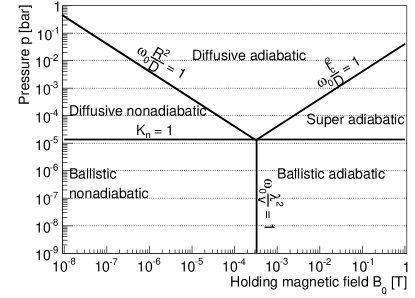
Figure 1: Classification of the different regimes for a $R=5$ cm radius spherical cell filled with polarized ³He gas as a function of pressure and holding magnetic field.

To illustrate this classification, let us consider some realistic systems of particular relevance for our study. The cylindrical RAL/Sussex/ILL trap Pendlebury et al. (2004), used to measure the neutron EDM, contains ultracold neutrons (UCN) and a mercury comagnetometer, immersed in a $1\leavevmode\nobreak\ \mathrm{\mu T}$ holding magnetic field. The small particles number of each species and the size of the trap ($47\leavevmode\nobreak\ \mathrm{cm}$ diameter and $12\leavevmode\nobreak\ \mathrm{cm}$ height) lead to a large Knudsen’s number and so to the ballistic regime. However, the speeds of the two particle species are very different: while the mercury atoms are at thermal equilibrium and have an average speed of several hundred meters per second, the UCN are moving at a few meters per second. Therefore the mercury comagnetometer is in the ballistic nonadiabatic regime whereas UCN are in the ballistic adiabatic limit. In the case of a gas at atmospheric pressure, such as a polarized ³He gas Petukhov et al. (2010), in a several $\mu\mathrm{{T}}$ holding field, the particle motion follows the diffusion equation and the number of Larmor precessions done by the spins between two collisions with the walls is very high. This kind of systems is thus in diffusive adiabatic regime.

As shown in Pignol and Roccia (2012); Guigue et al. (2014), the leading order of frequency shifts (9), (10) and (11) for adiabatic and nonadiabatic regimes can be expressed as powers of $\omega_{0}\tau_{\mathrm{corr}}$ or $1/\omega_{0}\tau_{\mathrm{corr}}$. To do so, we apply a succession of integrations by parts of the integrals defining the frequency shifts. This is the purpose of the two next sections. The first one presents the simplified expression of the frequency shift in the adiabatic regime. The nonadiabatic regime will be considered in the second next section. The well-known case of uniform magnetic gradients will be discussed in Section VI.

IV Adiabatic regime: high magnetic field or slow particles, arbitrary fields

The adiabatic regime corresponds to systems which satisfy $\omega_{0}\gg 1/\tau_{\mathrm{corr}}$. We want to expand the frequency shift (7) in power series of $1/\omega_{0}$. One way to obtain such an expression consists in applying several integrations by parts

$$\int_{0}^{\infty}\sin(\omega_{0}\tau)f(\tau)\mathrm{d}\tau=\left[\frac{-\cos(\omega_{0}\tau)}{\omega_{0}}f(\tau)\right]_{0}^{\infty}+\frac{1}{\omega_{0}}\int_{0}^{\infty}\cos(\omega_{0}\tau)\frac{\mathrm{d}f}{\mathrm{d}\tau}(\tau)\mathrm{d}\tau,$$ (15)

$$\int_{0}^{\infty}\cos(\omega_{0}\tau)f(\tau)\mathrm{d}\tau=\left[\frac{\sin(\omega_{0}\tau)}{\omega_{0}}f(\tau)\right]_{0}^{\infty}-\frac{1}{\omega_{0}}\int_{0}^{\infty}\sin(\omega_{0}\tau)\frac{\mathrm{d}f}{\mathrm{d}\tau}(\tau)\mathrm{d}\tau.$$ (16)

Equation (15) and (16) assume that the function $f$ and its derivative are integrable. We denote $\dot{f}=\frac{\mathrm{d}f}{\mathrm{d}\tau}$. Using the fact that the correlation functions go to zero at infinite time, we can write

$$\delta\omega_{B^{2}} = \frac{\gamma^{2}}{2\omega_{0}}\langle b_{x}^{2}+b_{y}^{2}\rangle-\frac{\gamma^{2}}{2\omega_{0}^{3}}\langle b_{x}(0)\ddot{b}_{x}(0)+b_{y}(0)\ddot{b}_{y}(0)\rangle$$ (17)

$$- \frac{\gamma^{2}}{2\omega_{0}^{3}}\int_{0}^{\infty}\cos(\omega_{0}\tau)\langle b_{x}(0)\dddot{b}_{x}(\tau)+b_{y}(0)\dddot{b}_{y}(\tau)\rangle\mathrm{d}\tau,$$

$$\delta\omega_{E^{2}} = \frac{\gamma^{2}E^{2}}{2c^{4}\omega_{0}}\langle v_{x}^{2}+v_{y}^{2}\rangle$$ (18)

$$+ \frac{\gamma^{2}E^{2}}{2c^{4}\omega_{0}}\int_{0}^{\infty}\cos(\omega_{0}\tau)\langle v_{x}(0)\dot{v}_{x}(\tau)+v_{y}(0)\dot{v}_{y}(\tau)\rangle\mathrm{d}\tau,$$

$$\delta\omega_{BE} = \frac{\gamma^{2}E}{c^{2}\omega_{0}^{2}}\langle b_{x}(0)\dot{v}_{x}(0)+b_{y}(0)\dot{v}_{y}(0)\rangle$$ (19)

$$- \frac{\gamma^{2}E}{c\omega_{0}^{2}}\int_{0}^{\infty}\cos(\omega_{0}\tau)\langle b_{x}(0)\ddot{v}_{x}(0)+b_{y}(0)\ddot{v}_{y}(0)\rangle\mathrm{d}\tau.$$

Making the reasonable assumption that the correlation functions and their derivatives are continuously decaying to 0 for $\tau\rightarrow\infty$, we apply the Riemann-Lebesgue lemma Appel (2007) and arrive at the conclusion that the last terms in Eq. (17), (18), (19) go to zero faster than the other terms in each equation. The frequency shift expressions can be written as (see also Eq. (27), (28), (29)):

$$\delta\omega_{B^{2}}=\frac{\gamma^{2}}{2\omega_{0}}\langle b_{x}^{2}+b_{y}^{2}\rangle-\frac{\gamma^{2}}{2\omega_{0}^{3}}\langle b_{x}(0)\ddot{b}_{x}(0)+b_{y}(0)\ddot{b}_{y}(0)\rangle+O\left(1/(\omega_{0}\tau_{\mathrm{corr}})^{5}\right),$$ (20)

$$\delta\omega_{E^{2}}=\frac{\gamma^{2}E^{2}}{2c^{4}\omega_{0}}\left\langle v_{x}^{2}+v_{y}^{2}\right\rangle+O\left(1/(\omega_{0}\tau_{\mathrm{corr}})^{3}\right),$$ (21)

$$\delta\omega_{BE}=\frac{\gamma^{2}E}{c^{2}\omega_{0}^{2}}\langle b_{x}(0)\dot{v}_{x}(0)+b_{y}(0)\dot{v}_{y}(0)\rangle+O\left(1/(\omega_{0}\tau_{\mathrm{corr}})^{4}\right).$$ (22)

Using the expressions for the derivatives of the correlation functions presented in the Appendix and assuming that velocities in different directions are uncorrelated and $\langle v_{x}^{2}\rangle=\langle v_{y}^{2}\rangle=\langle v_{z}^{2}\rangle=\frac{1}{3}\langle v^{2}\rangle$, we obtain

$$\delta\omega_{B^{2}} = \frac{\gamma^{2}}{2\omega_{0}}\langle b_{x}^{2}+b_{y}^{2}\rangle+\frac{\gamma^{2}}{6\omega_{0}^{3}}\langle v^{2}\rangle\langle|\vec{\nabla}b_{x}|^{2}+|\vec{\nabla}b_{y}|^{2}\rangle+O\left(1/(\omega_{0}\tau_{\mathrm{corr}})^{5}\right),$$ (23)

$$\delta\omega_{E^{2}}=\frac{\gamma^{2}E^{2}}{3c^{4}\omega_{0}}\langle v^{2}\rangle+O\left(1/(\omega_{0}\tau_{\mathrm{corr}})^{3}\right),$$ (24)

$$\delta\omega_{BE}=\frac{\gamma^{2}E}{c^{2}\omega_{0}^{2}}\left(\langle\frac{\partial b_{x}}{\partial x}\,v_{x}^{2}\rangle+\langle\frac{\partial b_{y}}{\partial y}\,v_{y}^{2}\rangle\right)+O\left(1/(\omega_{0}\tau_{\mathrm{corr}})^{4}\right).$$ (25)

These results are presented in Table 1. The first term in Eq. (23) corresponds to the leading order of the frequency shift in adiabatic regime Guigue et al. (2014).

It is instructive to note that these results can be obtained in another way. One can rewrite Eq. (6)

$$S_{ij}(\omega)=\int_{0}^{\infty}e^{i\omega\tau}\langle B_{i}(0)B_{j}(\tau)\rangle\mathrm{d}\tau=\int_{0}^{\infty}e^{i\omega\tau}f(\tau)\mathrm{d}\tau$$ (26)

and expand $f(\tau)$ in a Taylor series

$$S_{ij}(\omega) = \int_{0}^{\infty}\left(f(0)+\dot{f}(0)\tau+\cdots+f^{(n)}(0)\frac{\tau^{n}}{n!}\right)e^{i\omega\tau}\mathrm{d}\tau$$ (27)

$$= \left(f(0)+\dot{f}(0)\frac{\partial}{\partial(i\omega)}+\cdots+\frac{f^{(n)}(0)}{n!}\frac{\partial^{n}}{\partial(i\omega)^{n}}\right)\int_{0}^{\infty}e^{i\omega t}d\tau$$

$$= f(0)\frac{i}{\omega}-\dot{f}(0)\frac{1}{\omega^{2}}+\ddot{f}(0)\frac{1}{i\omega^{3}}+\cdots+f^{(n)}(0)\frac{(-1)^{n}}{\omega^{n+1}i^{n-1}}.$$

Taking the real part (that is, the relaxation rate for the $B^{2},E^{2}$ terms and the frequency shift for the $EB$ term, we obtain

$$\mathrm{Re}\left[S_{ij}(\omega)\right]=-\dot{f}(0)\frac{1}{\omega^{2}}+\frac{\dddot{f}(0)}{\omega^{4}}+\cdots,$$ (28)

which is equivalent to Eq. (14) of Guigue et al. (2014) and (19) above but now we have another form of the correction term and we can use this to calculate the frequency range where the first term is a good approximation. For the imaginary part ($B^{2},E^{2}$ frequency shifts and $EB$ relaxation) we find

$$\mathrm{Im}\left[S_{ij}(\omega)\right]=\frac{f(0)}{\omega}-\frac{\ddot{f}(0)}{\omega^{3}}+\cdots,$$ (29)

which is equivalent to Eq. (17) of the same paper and Eq. (20) above. In addition we find,

$$\Gamma_{1(B^{2})} =\gamma^{2}\left[-\frac{1}{\omega_{0}^{2}}\langle b_{x}(0)\dot{b}_{x}(0)+b_{y}(0)\dot{b}_{y}(0)\rangle+\frac{1}{\omega_{0}^{4}}\langle b_{x}(0)\dddot{b}_{x}(0)+b_{y}(0)\dddot{b}_{y}(0)\rangle\right],$$ (30)

$$\Gamma_{1(E^{2})} =\frac{\gamma^{2}E^{2}}{c^{4}}\left[-\frac{1}{\omega_{0}^{2}}\langle v_{x}(0)\dot{v}_{x}(0)+v_{y}(0)\dot{v}_{y}(0)\rangle+\frac{1}{\omega_{0}^{4}}\langle v_{x}(0)\dddot{v}_{x}(0)+v_{y}(0)\dddot{v}_{y}(0)\rangle\right],$$ (31)

$$\Gamma_{1(BE)} =\frac{2\gamma^{2}E}{c^{2}}\left[\frac{1}{\omega_{0}}\langle b_{x}(0)v_{x}(\tau)+b_{y}(0)v_{y}(\tau)\rangle\mathrm{|}_{\tau=0}+\frac{1}{\omega_{0}^{3}}\langle b_{x}(0)\ddot{v}_{x}(0)+b_{y}(0)\ddot{v}_{y}(0)\rangle\right].$$ (32)

Using the results presented in the Appendix, we can write

$$\Gamma_{1(B^{2})} =-\frac{\gamma^{2}}{2\omega_{0}^{2}}\langle\vec{v}\cdot\vec{\nabla}\left(b_{x}^{2}+b_{y}^{2}\right)\rangle+O\left(1/\left(\omega_{0}\tau_{\mathrm{corr}}\right)^{4}\right),$$ (33)

$$\Gamma_{1(E^{2})} =-\frac{\gamma^{2}E^{2}}{\omega_{0}^{2}c^{4}}\langle v_{x}\dot{v}_{x}+v_{y}\dot{v}_{y}\rangle+O\left(1/(\omega_{0}\tau_{\mathrm{corr}})^{4}\right)$$ (34)

$$\Gamma_{1(BE)} =\frac{2\gamma^{2}E}{\omega_{0}c^{2}}\langle b_{x}v_{x}+b_{y}v_{y}\rangle+O\left(1/(\omega_{0}\tau_{\mathrm{corr}})^{3}\right)$$ (35)

We expressed the correlation function derivatives in (23), (24), (25), (33) and (35) as volume averages of the velocity and magnetic field, in the adiabatic limit. These expressions are therefore independent of the particle motion in the cell. The high frequency limits for $\delta\omega_{B^{2}}$, $\delta\omega_{E^{2}}$, $\Gamma_{1(B^{2})}$ and $\Gamma_{1(BE)}$ are universal.

The first term in (33) behaves as $1/\omega_{0}^{2}$ and has been calculated in Guigue et al. (2014) in the diffusive adiabatic regime. However the diffusion theory breaks down at times shorter than the collision time $\tau_{\rm{coll}}$, so that at high frequencies, ($\omega_{0}\tau_{\rm{coll}}\gg 1$) the spectrum deviates from that expected on the basis of diffusion theory. The high frequency (super-adiabatic) limit is correctly given by Swank et al. (2012), using a correlation function that is valid for all times, namely the first term in (33) goes to zero as the velocity is initially uncorrelated with position, and the very high frequency behavior goes as $\left(1/\omega_{0}^{4}\right)$. The result of Swank et al. (2012) shows how the behavior goes from the $\left(\sim 1/\omega_{0}^{2}\right)$ predicted by diffusion theory at high frequencies to $\left(\sim 1/\omega_{0}^{4}\right)$ as $\omega_{0}\tau_{\rm{coll}}$ becomes on the order of or greater than 1.

V Nonadiabatic regime: weak magnetic field or fast particles, arbitrary fields

We now consider the nonadiabatic limit $\omega_{0}\tau_{\mathrm{corr}}\ll 1$. To expand the frequency shifts expressions in terms of power of $\omega_{0}$, we simply apply the same procedure of recursive integrations by parts, changing the part that is integrated:

$$\int_{0}^{\infty}\sin(\omega_{0}\tau)f(\tau)\mathrm{d}\tau=\left[\sin(\omega_{0}\tau)\int_{0}^{\tau}f(t)\mathrm{d}t\right]_{0}^{\infty}-\omega_{0}\int_{0}^{\infty}\cos(\omega_{0}\tau)\int_{0}^{\tau}f(t)\mathrm{d}t\mathrm{d}\tau$$ (36)

$$\int_{0}^{\infty}\cos(\omega_{0}\tau)f(\tau)\mathrm{d}\tau=\left[\cos(\omega_{0}\tau)\int_{0}^{\tau}f(t)\mathrm{d}t\right]_{0}^{\infty}+\omega_{0}\int_{0}^{\infty}\sin(\omega_{0}\tau)\int_{0}^{\tau}f(t)\mathrm{d}t\mathrm{d}\tau.$$ (37)

When applying these relations to Eq. (9), (10) and (11), we obtain:

$$\delta\omega_{E^{2}}= -\frac{\gamma^{2}E^{2}}{2c^{4}}\omega_{0}\langle x^{2}+y^{2}\rangle$$

$$+\frac{\gamma^{2}E^{2}}{2c^{4}}\omega_{0}^{2}\int_{0}^{\infty}\sin(\omega_{0}\tau)\langle x(0)x(\tau)+y(0)y(\tau)\rangle d\tau$$ (38)

$$\delta\omega_{BE}= -\frac{\gamma^{2}E}{c^{2}}\langle b_{x}x+b_{y}y\rangle$$

$$+\frac{\gamma^{2}E}{c^{2}}\omega_{0}\int_{0}^{\infty}\sin(\omega_{0}\tau)\langle b_{x}(0)x(\tau)+b_{y}(0)y(\tau)\rangle d\tau.$$ (39)

One can see that the last terms on the right-hand sides of Eq. (38) and (39), as well as Eq. (9) involve Fourier transforms of correlation functions which depends exclusively on position. Since we are in the limit $\omega_{0}\tau_{\mathrm{corr}}\ll 1$ we need to consider only the first order expansion of the involved trigonometric functions: $\sin(\omega_{0}\tau)\approx\omega_{0}\tau$. (For times $\tau\gtrsim\tau_{\mathrm{corr}}$ the correlation function goes to zero.) Applying this method to Eq. (9), (38) and (39), we obtain

$$\delta\omega_{B^{2}}\approx\frac{\gamma^{2}}{2}\omega_{0}\int_{0}^{\infty}\tau\langle b_{x}(0)b_{x}(\tau)+b_{y}(0)b_{y}(\tau)\rangle\mathrm{d}\tau$$ (40)

$$\delta\omega_{E^{2}}\approx-\frac{\gamma^{2}E^{2}}{2c^{4}}\omega_{0}\langle x^{2}+y^{2}\rangle+\frac{\gamma^{2}E^{2}}{2c^{4}}\omega_{0}^{3}\int_{0}^{\infty}\tau\langle x(0)x(\tau)+y(0)y(\tau)\rangle\mathrm{d}\tau$$ (41)

$$\delta\omega_{BE}\approx -\frac{\gamma^{2}E}{c^{2}}\langle b_{x}x+b_{y}y\rangle$$ (42)

$$+\frac{\gamma^{2}E}{c^{2}}\omega_{0}^{2}\int_{0}^{\infty}\tau\langle b_{x}(0)x(\tau)+b_{y}(0)y(\tau)\rangle\mathrm{d}\tau.$$

The last terms in Eq. (41) and (42) can not be calculated for any arbitrary trap geometry. But one can see that they behave as $\omega_{0}^{2}\tau_{\mathrm{corr}}^{2}$ when $\omega_{0}\tau_{\mathrm{corr}}$ goes to zero. This means that the expressions of the frequency shifts are dominated by the first term on the right hand side. These results are presented in Table 1.

Similarly, since $\cos\omega_{0}\tau\approx 1$, Eq. (12), (13) and (14)) become

$$\Gamma_{1(B^{2})} =\gamma^{2}\int_{0}^{\infty}\langle b_{x}(0)b_{x}(\tau)+b_{y}(0)b_{y}(\tau)\rangle\mathrm{d}\tau,$$ (43)

$$\Gamma_{1(E^{2})} =\frac{\gamma^{2}E^{2}}{c^{4}}\omega_{0}^{2}\int_{0}^{\infty}\langle x(0)x(\tau)+y(0)y(\tau)\rangle\mathrm{d}\tau,$$ (44)

$$\Gamma_{1(BE)} =\frac{2\gamma^{2}E}{c^{2}}\omega_{0}\int_{0}^{\infty}\langle b_{x}(0)x(\tau)+b_{y}(0)y(\tau)\rangle\mathrm{d}\tau,$$ (45)

from which the low frequency limits follow immediately.

Frequency	Adiabatic	Nonadiabatic
shift	(UCNs)	(Hg)
$\delta\omega_{B^{2}}$	$\frac{\gamma^{2}}{2\omega_{0}}\langle b_{x}^{2}+b_{y}^{2}\rangle+\frac{\gamma^{2}}{6\omega_{0}^{3}}\langle v^{2}\rangle\langle|\vec{\nabla}b_{x}|^{2}+|\vec{\nabla}b_{y}|^{2}\rangle$	$\frac{\gamma^{2}}{2}\omega_{0}\int_{0}^{\infty}\tau\langle b_{x}(0)b_{x}(\tau)+b_{y}(0)b_{y}(\tau)\rangle\mathrm{d}\tau$
$\delta\omega_{E^{2}}$	$\frac{\gamma^{2}E^{2}}{3c^{4}\omega_{0}}\langle v^{2}\rangle$	$-\frac{\gamma^{2}E^{2}}{2c^{4}}\omega_{0}\langle x^{2}+y^{2}\rangle$
$\delta\omega_{BE}$	$-\frac{\gamma^{2}E}{c^{2}\omega_{0}^{2}}\left(\langle\frac{\partial b_{x}}{\partial x}\,v_{x}^{2}\rangle+\langle\frac{\partial b_{y}}{\partial y}\,v_{y}^{2}\rangle\right)$	$\frac{\gamma^{2}E}{c^{2}}\langle b_{x}x+b_{y}y\rangle$

Table 1: Expressions of the leading terms of the frequency shifts induced by the transverse magnetic and motional fields, in the adiabatic and nonadiabatic limits.

VI Magnetic field linearly dependent on position (uniform gradients)

In this case, which is what is usually treated theoretically and applies to most experimental situations, one can simplify the derivatives in terms of trajectory correlation functions without any evolution equation and derive a variety of relationships. Let us consider a magnetic inhomogeneity $\vec{b}$ dependent linearly on the position of a spin:

$$b_{x} =G_{x}x,$$ (46)

$$b_{y} =G_{y}y,$$ (47)

where the relation $G_{x}+G_{y}=-\frac{\partial b_{z}}{\partial z}=-G_{z}$ holds by the divergence theorem.

VI.1 General relations for fields with linear gradients and cylindrical symmetry

VI.1.1 Expressions relating frequency shifts with frequency shifts

In the common case of cylindrical field symmetry, (with arbitrary cell shape) the correlation functions of interest are $\langle v_{x}(0)v_{x}(\tau)+v_{y}(0)v_{y}(\tau)\rangle,$ $\langle x(0)v_{x}(\tau)+y(0)v_{y}(\tau)\rangle,$ $\langle x(0)x(\tau)+y(0)y(\tau)\rangle$ which satisfy the relations

$$\langle x(0)v_{x}(\tau)+y(0)v_{y}(\tau)\rangle =-\frac{d}{d\tau}\langle x(0)x(\tau)+y(0)y(\tau)\rangle,$$ (48)

$$\langle v_{x}(0)v_{x}(\tau)+v_{y}(0)v_{y}(\tau)\rangle =\frac{d}{d\tau}\langle x(0)v_{x}(\tau)+y(0)v_{y}(\tau)\rangle=-\frac{d^{2}}{d\tau^{2}}\langle x(0)x(\tau)+y(0)y(\tau)\rangle.$$ (49)

Then

$$S_{xv}\left(\omega\right) =-i\omega S_{xx}\left(\omega\right)+\left\langle x^{2}+y^{2}\right\rangle,$$ (50)

$$S_{vv}\left(\omega\right) =-i\omega S_{xv}\left(\omega\right).$$ (51)

According to Eq. (9, 10, 11) we find

$$\delta\omega_{BE}=K_{BE}\mathrm{Re}\left(S_{xv}(\omega)\right)=-K_{BE}\mathrm{Im}\left(S_{vv}(\omega)/\omega\right)=-\frac{K_{BE}}{K_{E^{2}}}\frac{\delta\omega_{E^{2}}}{\omega},$$ (52)

with $K_{BE}=\frac{\gamma^{2}G_{z}E}{2c^{2}}$, $K_{B^{2}}=\frac{\gamma^{2}G_{z}^{2}}{8}$, $K_{E^{2}}=\frac{\gamma^{2}E^{2}}{2c^{4}}$. The last expression was obtained in Pendlebury et al. (2004) for the case of particles moving in a cylinder with specular reflecting walls and no gas collisions, but our result holds for any cell shape and type of particle motion. Equation (39) can be written as

$$\delta\omega_{BE} =\frac{\gamma^{2}EG_{z}}{2c^{2}}\langle x^{2}+y^{2}\rangle-\frac{\gamma^{2}EG_{z}}{2c^{2}}\omega_{0}\int_{0}^{\infty}\sin(\omega_{0}\tau)\langle x(0)x(\tau)+y(0)y(\tau)\rangle d\tau$$ (53)

$$=\frac{\gamma^{2}EG_{z}}{2c^{2}}\langle x^{2}+y^{2}\rangle-\frac{4E\omega_{0}}{c^{2}G_{z}}\delta\omega_{B^{2}},$$ (54)

so that Eq. (54) represents a method of measuring the linear in E shift without applying an electric field. To do this one would apply a known constant gradient and look for a frequency shift dependent on the square of the gradient. The possibility of the volume average field being changed by application of the gradient can be accounted for by taking the part of the shift proportional to the square of the gradient. Another method would be to measure the relaxation rate due to then application of the gradient as discussed in the next paragraph.

VI.1.2 Expressions relating frequency shifts and relaxation rates

As the correlation functions defined in Eqs. (9 - 14) are all causal, that is, they are zero for $\tau<0$, their real and imaginary parts are related by a dispersion relation Papoulis (1962) and we can write

$$\delta\omega_{BE} =K_{BE}\left[\langle x^{2}+y^{2}\rangle-\omega\mathrm{Im}\left[S_{xx}\left(\omega\right)\right]\right]$$ (55)

$$=K_{BE}\left[\langle x^{2}+y^{2}\rangle-\frac{\omega}{\pi}\int_{-\infty}^{\infty}\frac{\mathrm{Re}\left[S_{xx}\left(\omega^{\prime}\right)\right]}{\omega-\omega^{\prime}}d\omega^{\prime}\right]$$ (56)

$$=K_{BE}\left[\langle x^{2}+y^{2}\rangle-\frac{\omega}{\pi}\frac{1}{2K_{B^{2}}}\int_{-\infty}^{\infty}\frac{\Gamma_{1\left(B^{2}\right)}}{\omega-\omega^{\prime}}d\omega^{\prime}\right]$$ (57)

$$=K_{BE}\left[\langle x^{2}+y^{2}\rangle-\frac{1}{K_{B^{2}}}\frac{\omega^{2}}{\pi}\int_{-\infty}^{\infty}\frac{\Gamma_{1\left(B^{2}\right)}\left(\omega^{\prime}\right)}{\omega^{2}-\omega^{\prime 2}}d\omega^{\prime}\right]$$ (58)

$$=K_{BE}\left[\langle x^{2}+y^{2}\rangle-\frac{1}{K_{E^{2}}}\frac{\omega^{2}}{\pi}\int_{-\infty}^{\infty}\frac{\Gamma_{1\left(E^{2}\right)}\left(\omega^{\prime}\right)}{\left(\omega^{2}-\omega^{\prime 2}\right)\omega^{\prime 2}}d\omega^{\prime}\right].$$ (59)

Equations (58) and (59) are particularly interesting because they allow measurement of the frequency dependence of $\delta\omega_{BE}$, the shift, linear in $E$, that produces a serious systematic error in the searches for particle electric dipole moments without application of an electric field. By applying a gradient, $\frac{\partial b_{z}}{\partial z},$ larger than any existing gradients and measuring $\Gamma_{1\left(B^{2}\right)}\left(\omega\right)$ one can reconstruct the frequency dependence of $\delta\omega_{BE}$. For the case of a non-cylindrically symmetric cell we can apply relatively large gradients $\partial b_{x,y}/\partial x,y$ and thus measure, separately, the spectra of the correlation functions in the two directions. While according to (58) we need to know the relaxation for all frequencies, the necessary range of measurement is limited because the known high and low frequency limits are reached rather quickly (30,43). Substituting (13) into (59) we obtain a form of the relation that has been obtained by another method in Lamoreaux and Golub (2005).

VI.1.3 Expressions relating relaxation rates with relaxation rates.

For completeness we give relations between the relaxation rates which are abtained in a similar way:

$$\Gamma_{1(E^{2})}=\frac{K_{E^{2}}}{K_{B^{2}}}\omega^{2}\Gamma_{1(B^{2})}=\frac{K_{E^{2}}}{K_{BE}}\omega\Gamma_{1(BE)}.$$ (60)

The relaxation caused by the electric field alone, $\Gamma_{1(E^{2})},$ has been discussed in Schmid et al. (2008).

VI.2 Adiabatic regime: high magnetic field or slow particles for fields with uniform gradients

We specify Eq. (23), (24), (25) to the case of a uniform gradient:

$$\delta\omega_{B^{2}}=\frac{\gamma^{2}}{2\omega_{0}}\langle b_{x}^{2}+b_{y}^{2}\rangle+\frac{\gamma^{2}}{2\omega_{0}^{3}}\left\{G_{x}^{2}\langle v_{x}^{2}\rangle+G_{y}^{2}\langle v_{y}^{2}\rangle\right\}+O(1/\omega_{0}^{5}\tau_{\mathrm{corr}}^{5})$$ (61)

$$\delta\omega_{E^{2}}=\frac{\gamma^{2}E^{2}}{2c^{4}\omega_{0}}\langle v_{x}^{2}+v_{y}^{2}\rangle+O(1/\omega_{0}^{3}\tau_{\mathrm{corr}}^{3})$$ (62)

$$\delta\omega_{BE}=-\frac{\gamma^{2}E}{c^{2}\omega_{0}^{2}}\left\{G_{x}\langle v_{x}^{2}\rangle+G_{y}\langle v_{y}^{2}\rangle\right\}+O(1/\omega_{0}^{4}\tau_{\mathrm{corr}}^{4}).$$ (63)

Similarly, the relaxation rates can be expressed as:

$$\Gamma_{1\left(B^{2}\right)} =-\gamma^{2}\frac{1}{\omega_{0}^{2}}\left[G_{x}^{2}\langle xv_{x}\rangle+G_{y}^{2}\langle yv_{y}\rangle\right]+O(1/\omega_{0}^{4}\tau_{\mathrm{corr}}^{4}),$$ (64)

$$\Gamma_{1\left(BE\right)} =\frac{2\gamma^{2}E}{c^{2}}\left[\frac{1}{\omega_{0}}\langle G_{x}xv_{x}+G_{y}yv_{y}\rangle+O(1/\omega_{0}^{3}\tau_{\mathrm{corr}}^{3})\right].$$ (65)

The first term in Eq. (61) corresponds to Eq. (18) in Guigue et al. (2014). It is remarkable that it is possible to derive a simple and universal expression for the third order term $\propto\omega_{0}^{-3}$ in Eq. (61). To our knowledge this third order term has never been calculated before.

VI.3 Low field, high velocity limit for fields with uniform gradients

For uniform gradients (47), the expression of $\delta\omega_{BE}$ (42) can be simplified to

$$\delta\omega_{BE} =-\frac{\gamma^{2}E}{c^{2}}\langle G_{x}x^{2}+G_{y}y^{2}\rangle+\frac{\gamma^{2}E}{c^{2}}\omega_{0}^{2}\int_{0}^{\infty}\tau\langle G_{x}x(0)x(\tau)+G_{y}y(0)y(\tau)\rangle\mathrm{d}\tau$$ (66)

$$=-\frac{\gamma^{2}E}{c^{2}}\langle G_{x}x^{2}+G_{y}y^{2}\rangle+O(\omega_{0}^{2}\tau_{\mathrm{corr}}^{2}).$$ (67)

Also (40) becomes

$$\delta\omega_{B^{2}}\approx\frac{\gamma^{2}}{2}\omega_{0}\int_{0}^{\infty}\tau\langle G_{x}^{2}x(0)x(\tau)+G_{y}^{2}y(0)y(\tau)\rangle\mathrm{d}\tau$$ (68)

and (41)

$$\delta\omega_{E^{2}}=-\frac{\gamma^{2}E^{2}}{2c^{4}}\omega_{0}\langle x^{2}+y^{2}\rangle+\frac{\gamma^{2}E^{2}}{2c^{4}}\omega_{0}^{3}\int_{0}^{\infty}\tau\langle x(0)x(\tau)+y(0)y(\tau)\rangle\mathrm{d}\tau.$$ (69)

Similarly

$$\Gamma_{1(B^{2})} =\gamma^{2}\int_{0}^{\infty}\langle G_{x}^{2}x(0)x(\tau)+G_{y}^{2}y(0)y(\tau)\rangle\mathrm{d}\tau,$$ (70)

$$\Gamma_{1(E^{2})} =\frac{\gamma^{2}E^{2}}{c^{4}}\omega_{0}^{2}\int_{0}^{\infty}\langle x(0)x(\tau)+y(0)y(\tau)\rangle\mathrm{d}\tau,$$ (71)

$$\Gamma_{1(BE)} =\frac{2\gamma^{2}E}{c^{2}}\omega_{0}\int_{0}^{\infty}\langle G_{x}x(0)x(\tau)+G_{y}y(0)y(\tau)\rangle\mathrm{d}\tau,$$ (72)

so that in the low frequency limit there are no universal or quasi-universal expressions.

VII Conclusion

In this paper we have investigated the asymptotic behavior of the spin-relaxation and related frequency shifts due to the restricted motion of particles in non-uniform magnetic and electric fields. Simple universal expressions (valid for any form of gas container and any spatial form of the field) were obtained for the observables $\delta\omega$ and $\Gamma_{1}$ for adiabatic and nonadiabatic regimes of spin - motion. The remarkable feature of all our results is that they were obtained without any specific assumptions about the explicit form of the correlation functions. Hence, we expect that our results are valid for both diffusive and ballistic regimes of motion. These results can then be applied to a wide variety of realistic systems. They are especially important in the context of experiments searching for the electric dipole moment using trapped particles, for the frequency shifts proportional to electric fields are of utmost importance. In particular we have given general relations between various frequency shifts and relaxation rates.

VIII Acknowledgment

The authors would like to thank Albert Steyerl for pointing out a numerical error in the first verision of the manuscript.

Appendix A Useful expressions of correlation functions

We derive three useful relations for the derivative of certain correlation functions in terms of volume averages. Let us consider an inhomogeneity $b_{i}$ with $i=x$ or $y$.

$$\frac{\mathrm{d}}{\mathrm{d}\tau}\langle b_{i}(0)b_{i}(\tau)\rangle|_{\tau=0} =\langle b_{i}(0)\dot{b}_{i}(0)\rangle$$ (73)

$$=\langle b_{i}\vec{\nabla}b_{i}\cdot\frac{\mathrm{d}\vec{r}}{\mathrm{d}\tau}\rangle$$ (74)

$$=\langle b_{i}\frac{\partial b_{i}}{\partial x}v_{x}\rangle+\langle b_{i}\frac{\partial b_{i}}{\partial y}v_{y}\rangle+\langle b_{i}\frac{\partial b_{i}}{\partial z}v_{z}\rangle$$ (75)

$$=\frac{1}{2}\langle\vec{v}\cdot\vec{\nabla}b_{i}^{2}\rangle$$ (76)

$$\frac{\mathrm{d}^{2}}{\mathrm{d}\tau^{2}}\langle b_{i}(0)b_{i}(\tau)\rangle|_{\tau=0} =\langle b_{i}(0)\ddot{b_{i}}(0)\rangle$$ (77)

$$=-\langle\dot{b_{i}}(0)\dot{b_{i}}(0)\rangle$$ (78)

$$=-\langle\left(\vec{\nabla}b_{i}\cdot\frac{\mathrm{d}\vec{r}}{\mathrm{d}\tau}\right)^{2}\rangle$$ (79)

$$=\langle\left(\frac{\partial b_{i}}{\partial x}v_{x}\right)^{2}\rangle+\langle\left(\frac{\partial b_{i}}{\partial y}v_{y}\right)^{2}\rangle+\langle\left(\frac{\partial b_{i}}{\partial z}v_{z}\right)^{2}\rangle$$ (80)

$$=\langle\left(\frac{\partial b_{i}}{\partial x}\right)^{2}\rangle\langle v_{x}^{2}\rangle+\langle\left(\frac{\partial b_{i}}{\partial y}\right)^{2}\rangle\langle v_{y}^{2}\rangle+\langle\left(\frac{\partial b_{i}}{\partial z}\right)^{2}\rangle\langle v_{z}^{2}\rangle$$ (81)

$$\frac{\mathrm{d}}{\mathrm{d}\tau}\langle b_{i}(0)v_{j}(\tau)\rangle|_{\tau=0} =-\langle\dot{b_{i}(0)}v_{j}(0)\rangle=-\langle(\vec{\nabla}b_{i}\cdot\vec{v})v_{j}\rangle$$ (82)

$$=-\langle\frac{\partial b_{i}}{\partial j}\,v_{j}^{2}\rangle$$ (83)

References

- Bloembergen et al. (1948) N. Bloembergen, E. Purcell, and R. Pound, Physical Review 73, 679 (1948).
- Wangsness and Bloch (1953) R. Wangsness and F. Bloch, Physical Review 89, 728 (1953).
- Bloch (1956) F. Bloch, Physical Review 102, 104 (1956).
- Redfield (1957) A. G. Redfield, IBM Journal of Research and Development 1, 19 (1957).
- Redfield (1965) A. G. Redfield, Advances in Magnetic Resonance 1, 1 (1965).
- Slichter (1964) C. P. Slichter, Principles of Magnetic Resonance (Harper&Row, 1964), ISBN 3540501576.
- Torrey (1956) H. Torrey, Physical Review 104, 563 (1956).
- Cates et al. (1988) G. D. Cates, S. R. Schaefer, and W. Happer, Physical Review A 37, 2877 (1988).
- McGregor (1990) D. D. McGregor, Physical Review A 41, 2631 (1990).
- Golub et al. (2011) R. Golub, R. M. Rohm, and C. M. Swank, Physical Review A 83, 023402 (2011).
- Nicholas et al. (2010) M. P. Nicholas, E. Eryilmaz, F. Ferrage, D. Cowburn, and R. Ghose, Progress in nuclear magnetic resonance spectroscopy 57, 111 (2010).
- Lamoreaux and Golub (2009) S. K. Lamoreaux and R. Golub, Journal of Physics G: Nuclear and Particle Physics 36, 104002 (2009).
- Eckel et al. (2013) S. Eckel, P. Hamilton, E. Kirilov, H. W. Smith, and D. DeMille, Phys. Rev. A 87, 052130 (2013).
- Pendlebury et al. (2004) J. Pendlebury, W. Heil, Y. Sobolev, P. Harris, J. Richardson, R. Baskin, D. Doyle, P. Geltenbort, K. Green, M. van der Grinten, et al., Physical Review A 70, 032102 (2004).
- Lamoreaux and Golub (2005) S. K. Lamoreaux and R. Golub, Physical Review A 71, 032104 (2005).
- Barabanov et al. (2006) A. L. Barabanov, R. Golub, and S. K. Lamoreaux, Physical Review A 74, 052115 (2006).
- Petukhov et al. (2010) A. K. Petukhov, G. Pignol, D. Jullien, and K. H. Andersen, Physical Review Letters 105, 170401 (2010).
- Clayton (2011) S. M. Clayton, Journal of magnetic resonance 211, 89 (2011).
- Swank et al. (2012) C. M. Swank, A. K. Petukhov, and R. Golub, Physics Letters A 376, 2319 (2012).
- Afach et al. (2015) S. Afach, C. A. Baker, G. Ban, G. Bison, K. Bodek, Z. Chowdhuri, M. Daum, M. Fertl, B. Franke, P. Geltenbort, et al., European Physical Journal D 69, 225 (2015).
- Pignol and Roccia (2012) G. Pignol and S. Roccia, Physical Review A 85, 042105 (2012).
- Guigue et al. (2014) M. Guigue, G. Pignol, R. Golub, and A. K. Petukhov, Physical Review A 90, 013407 (2014).
- Appel (2007) W. Appel, Mathematics for Physics and Physicists (2007), ISBN 978-0691131023.
- Papoulis (1962) A. Papoulis, The Fourier integral and its applications, McGraw-Hill electronic sciences series (McGraw-Hill, New York, San Francisco, London, 1962), ISBN 0-07-048447-3.
- Schmid et al. (2008) R. Schmid, B. Plaster, and B. W. Filippone, Physical Review A 78, 023401 (2008).