Self-dual configurations in Abelian Higgs models with $k$-generalized gauge field dynamics

Abstract

We have shown the existence of self-dual solutions in new Maxwell-Higgs scenarios where the gauge field possesses a $k$-generalized dynamic, i.e., the kinetic term of gauge field is a highly nonlinear function of $F_{\mu\nu}F^{\mu\nu}$. We have implemented our proposal by means of a $k$-generalized model displaying the spontaneous symmetry breaking phenomenon. We implement consistently the Bogomol’nyi-Prasad-Sommerfield formalism providing highly nonlinear self-dual equations whose solutions are electrically neutral possessing total energy proportional to the magnetic flux. Among the infinite set of possible configurations, we have found families of $k$-generalized models whose self-dual equations have a form mathematically similar to the ones arising in the Maxwell-Higgs or Chern-Simons-Higgs models. Furthermore, we have verified that our proposal also supports infinite twinlike models with $|\phi|^{4}$-potential or $|\phi|^{6}$-potential. With the aim to show explicitly that the BPS equations are able to provide well-behaved configurations, we have considered a test model in order to study axially symmetric vortices. By depending of the self-dual potential, we have shown that the $k$-generalized model is able to produce solutions that for long distances have a exponential decay (as Abrikosov-Nielsen-Olesen vortices) or have a power-law decay (characterizing delocalized vortices). In all cases, we observe that the generalization modifies the vortex core size, the magnetic field amplitude and the bosonic masses but the total energy remains proportional to the quantized magnetic flux.

I Introduction

Configurations exhibiting nontrivial topology usually emerge as static solutions of classical fields models presenting highly nonlinear interactions. In general, this nonlinearity is introduced by means of a potential describing the scalar-matter self-interaction n5 . Moreover, the potential must allow the mechanism of the spontaneous symmetry breaking happen, because it is known that the topological structures are formed during symmetry-breaking phase transitions. It is the reason why these solutions receive so much attention within the cosmological context or condensed matter physics.

In the last years have received a special attention the topological objects arising from noncanonical field models, some of them coming from string theories. These new field theories (called $k$-generalized models) are characterized by possess nonstandard kinetic terms that could play the role of a symmetry breaking potential o1 ; MHgeral . The new self-dual $k$-generalized solutions can exhibit similar behavior as their conventional counterparts however the exotic dynamics can also produce variations on the vortex-core size and on the field amplitudes o2 . Furthermore, some $k$-models possesses the same self-dual configurations (they have exactly the same BPS equations), including their energy density and total energy than their canonical counterparts, they are named are named twinlike models n007 ; n009 ; n008 ; n010 . Such a versatility has motivated the use of nonstandard kinetic terms in an attempt to explain the accelerated inflationary phase of the universe n8 , strong gravitational waves sgw , dark matter dm , and others o .

There are many scenarios motivating the study of the generalized Maxwell-Higgs models. Among them we can cite the problem of the localization of gravity and/or particle/field in a 6-D braneworld massimo and the Born-Infeld-Higgs models BI_1 ; Diego . Another interesting scenario for to study Maxwell-Higgs models is related to cosmic strings, topological defects similar to the vortices, which may have great importance in the evolution of the Cosmos and formation of the structures existing in the Universe Vilenkin . The community has renewed its interest because recently it was established that superstrings theory supports cosmic strings solutions inside its theoretical framework Sakellariadou .

The aim of the present manuscript is go further in the study of self-dual configurations in noncanonical models by considering a Maxwell-Higgs (MH) scenario where the $k$-generalization is driven by the gauge field kinetic term, i.e., the kinetic term of gauge field is a highly nonlinear function of $F_{\mu\nu}F^{\mu\nu}$. We have organized our contribution as follows: In Sec. II we establish the theoretical framework in which our studies will be developed. We implement consistently the Bogomol’nyi-Prasad-Sommerfield formalism n4 providing highly nonlinear self-dual equations whose solutions are electrically neutral possessing total energy proportional to the magnetic flux. It was verified $k$-generalized framework supports infinity twinlike self-dual models with $|\phi|^{4}$ or $|\phi|^{6}$ potentials. In Sec. III we have managed to establishing a class of models whose BPS equations become linear in the magnetic field, i.e., they have mathematical expressions very similar to the self-dual equations corresponding to the Maxwell-Higgs or Chern-Simons-Higgs models. In Sec. IV, we study the general properties of the axially symmetric vortex solutions generated by an arbitrary $k$-generalized Abelian-Higgs model with $|\phi|^{4}$ and $|\phi|^{6}$ potentials. We have also propose a general potential generating self-dual delocalized vortex whose behavior for long distances is type a power decay. Finally, in Sec. V, we present our ending comments and perspectives.

II Abelian Higgs models with $k$-generalized gauge field dynamics

Our proposal consists of a possible generalized model where the $k$-generalization idea is applied only to the dynamics of the gauge field. We introduce an approach based in models supporting spontaneous symmetry breaking potentials described by the following Lagrangian density,

$$\mathcal{L}=h(|\phi|)K(Y)+w(|\phi|)\left|D_{\mu}\phi\right|^{2}-V(|\phi|),$$ (1)

where the complex scalar field $\phi$ stands for the Higgs one whose minimal covariant derivative reading as $D_{\mu}\phi=\partial_{\mu}\phi-ieA_{\mu}\phi$, with $A_{\mu}$ being the gauge field. In the gauge field sector $h(|\phi|)$ is a nonnegative function and $K(Y)$ driving the $k$-generalization of the gauge field is an arbitrary and nonpositive function of $Y$ which is defined by

$$Y\equiv-\frac{F_{\mu\nu}F^{\mu\nu}}{4\mathcal{U}(|\phi|)},$$ (2)

being $F_{\mu\nu}=\partial_{\mu}A_{\nu}-\partial_{\nu}A_{\mu}$ the electromagnetic field strength tensor. In the Higgs sector, $w(|\phi|)$ must be positive, whilst $V(|\phi|)$ represents some convenient potential. The Lagrangian density (1) allows to describe many of the generalized models present in the literature, for example, we can recover Born-Infeld-Higgs ones BI_1 ; Diego , the prototype of highly nonlinear gauge field dynamics.

In the remainder of the manuscript we are interested in the self-dual configurations can be generated by these $k$-generalized models by considering $w(|\phi|)=1$. Thus, we consider the $k$-generalized models defined by the Lagrangian density,

$$\mathcal{L}=h(|\phi|)K(Y)+\left|D_{\mu}\phi\right|^{2}-V(|\phi|).$$ (3)

The equation of motion of the gauge field reads

$$\partial_{\nu}\left(\frac{h}{\mathcal{U}}K_{Y}F^{\nu\mu}\right)=eJ^{\mu},$$ (4)

where $K_{Y}\equiv dK/dY$ and $J_{\mu}$ is the conserved current density given by

$$J_{\mu}=i\left(\phi\partial_{\mu}\phi^{\ast}-\phi^{\ast}\partial_{\mu}\phi\right)-2eA_{\mu}\left|\phi\right|^{2}.$$ (5)

The equation of motion for the Higgs field is

$$D_{\mu}D^{\mu}\phi-K\frac{\partial h}{\partial\phi^{\ast}}+\frac{h}{\mathcal{U}}YK_{Y}\frac{\partial\mathcal{U}}{\partial\phi^{\ast}}+\frac{\partial V}{\partial\phi^{\ast}}=0.$$ (6)

From equation (4) we obtain the Gauss and Ampère laws for time independent solutions,

$$\partial_{j}\left(\frac{h}{\mathcal{U}}K_{Y}\partial_{j}A_{0}\right)=2e^{2}A_{0}\left|\phi\right|^{2},\\$$ (7)

$$\epsilon_{kj}\partial_{j}\left(\frac{h}{\mathcal{U}}K_{Y}B\right)=eJ_{k},$$ (8)

respectively.

From the Gauss law, the electric charge density is given by $J_{0}=-2e{2}A_{0}\left|\phi\right|^{2}$ whose integral provides null total electric charge,

$$Q=\int d^{2}xJ_{0}=0.$$ (9)

It can be proved directly by integrating the Gauss law under suitable boundary conditions, i.e., for $|x|\rightarrow\infty$, $A_{0}\rightarrow 0$ and $|\phi|\rightarrow cte.$ Therefore, the field configurations are electrically neutral.

We observe that for such configurations the gauge condition $A_{0}=0$ is compatible with the Gauss. Consequently, for this gauge condition, the Higgs field equation reduces to be

$$D_{k}D_{k}\phi+K\frac{\partial h}{\partial\phi^{\ast}}-\frac{h}{\mathcal{U}}YK_{Y}\frac{\partial\mathcal{U}}{\partial\phi^{\ast}}-\frac{\partial V}{\partial\phi^{\ast}}=0.$$ (10)

II.1 The BPS formalism

The energy-momentum tensor for the models described by the Lagrangian density (3) is

$$T_{\mu\nu} = -\frac{h}{\mathcal{U}}K_{Y}F_{\mu\beta}F_{\nu}{}^{\beta}+(D_{\mu}\phi)^{\ast}D_{\nu}\phi$$

$$+(D_{\nu}\phi)^{\ast}D_{\mu}\phi-\eta_{\mu\nu}\mathcal{L}.$$

The energy is given by the integration of the $T_{00}$ component which for time-independent configurations with $A_{0}=0$ reads,

$$E=\int d^{2}x\left[\frac{{}}{{}}-hK+\left|D_{k}\phi\right|^{2}+V\right].$$ (12)

It is positive-definite due to the conditions previously imposed to the functions $h(|\phi|)$ and $K(Y)$.

We begin the implementation of the BPS formalism n4 by introducing the identity

$$\left|D_{k}\phi\right|^{2}=\left|D_{\pm}\phi\right|^{2}\pm eB\left|\phi\right|^{2}\pm\frac{1}{2}\epsilon_{ik}\partial_{i}J_{k},$$ (13)

into the total energy (12) that after some algebraic manipulations can expressed as

$$E = \int d^{2}x\left[\left|D_{\pm}\phi\right|^{2}+\frac{\mathcal{U}}{2hK_{Y}}\left(\frac{h}{\mathcal{U}}K_{Y}B\mp\sqrt{W}\right)^{2}\right.$$

$$\hskip 35.56593pt\pm B\left(\sqrt{W}+e\left|\phi\right|^{2}\right)\pm\frac{1}{2}\epsilon_{ik}\partial_{i}J_{k}$$

$$\hskip 35.56593pt\left.-\frac{\mathcal{U}}{2hK_{Y}}W-\frac{1}{2}\frac{h}{\mathcal{U}}K_{Y}B^{2}-hK+V\right],$$

where we have introduced the function $W(|\phi|)$ that will be determined later. At this point, we remember that the BPS formalism consist in expressing the energy density as a sum of quadratic terms plus a term proportional to the magnetic field plus a total derivative. In our case, such requirements are achieved in two steps: The first one consists in to determine $W(|\phi|)$ by choosing that the factor multiplying the magnetic field in (II.1) to be $ev^{2}=cte.$, thus, we get

$$W=e^{2}\left(v^{2}-\left|\phi\right|^{2}\right)^{2}.$$ (15)

A second step is to require that the third row in (II.1) be null,

$$\frac{\mathcal{U}}{2hK_{Y}}W+\frac{1}{2}\frac{h}{\mathcal{U}}K_{Y}B^{2}+hK-V=0,$$ (16)

establishing a relation between all the functions defining the generalized model. Importantly that the Eq. (16) it is not arbitrary because, as we will see later, in the BPS limit, it becomes equivalent to the condition: $T_{11}+T_{22}=0$, proposed by Schaposnik and Vega SV to obtain self-dual configurations.

By fulfilling the conditions (15) and (16), the energy (II.1) is written as

$$E = \int d^{2}x\left\{\pm ev^{2}B\pm\frac{1}{2}\epsilon_{ik}\partial_{i}J_{k}+\left|D_{\pm}\phi\right|^{2}\frac{{}}{{}}\right.$$

$$\hskip 31.2982pt\left.+\frac{\mathcal{U}}{2hK_{Y}}\left[\frac{h}{\mathcal{U}}K_{Y}B\mp e\left(v^{2}-\left|\phi\right|^{2}\right)\right]^{2}\right\}.$$

The integration of the first term in Eq. (II.1) provides the total magnetic flux,

$$\int d^{2}xB=\Phi,$$ (18)

and, under suitable boundary conditions, the integration of the total derivative in Eq. (II.1) gives null contribution to the energy.

Then, from Eq. (II.1), we can see that total energy has a lower bound

$$E\geq\pm ev^{2}\Phi,$$ (19)

which is attained by field configurations satisfying the BPS or self-dual equations,

$$D_{\pm}\phi=0,$$ (20)

$$\frac{h}{\mathcal{U}}K_{Y}B=\pm e\left(v^{2}-\left|\phi\right|^{2}\right).$$ (21)

Besides, the Eqs. (16) in the BPS limit becomes

$$\frac{h}{\mathcal{U}}K_{Y}B^{2}+hK-V=0,$$ (22)

which corresponds exactly to the condition $T_{11}+T_{22}=0$, from the Schaposnik and Vega formalism. It also allows us to determine explicitly the self-dual potential,

$$V_{sd}=\frac{h}{\mathcal{U}}K_{Y}B^{2}+hK\geq 0,$$ (23)

where $K_{Y}$ must be a positive function.

Finally, from Eq. (12) we obtain the energy density of the solutions satisfying the Bogomol’nyi bound (19), i. e., the field configurations are solutions the self-dual equations (20) and (21),

$$\varepsilon_{{}_{BPS}}=\frac{h}{\mathcal{U}}K_{Y}B^{2}+|D_{k}\phi|^{2}.$$ (24)

It will be positive-definite since the functions $h(|\phi|)$, $\mathcal{U}(|\phi|)$ and $K_{Y}(Y)$ also are.

It can be verified that the BPS equations (20) and (21) also solve the second-order Euler-Lagrange equations given by Eqs. (8) and (10) when the potential (23) is considered.

II.2 Self-dual configurations with $k$-generalized gauge field dynamics without an explicit SSB potential

The results obtained for the model (3) can be used to analyze the interesting case when there is no an explicit spontaneous symmetry breaking potential. Such a situation is obtained by setting $V(|\phi|)=0$ and $h(|\phi|)=\mathcal{U}(|\phi|)$ resulting in the following Lagrangian density,

$$\mathcal{L}=\mathcal{U}(|\phi|)K(Y)+\left|D_{\mu}\phi\right|^{2}.$$ (25)

Obviously, the equations of motion for both gauge and Higgs fields are modified, but the configurations remain electrically neutral. The self-dual configurations have the total energy (19) and they are described by the following BPS or self-dual equations: The first one is exactly the Eq. (20) and the second one is obtained from (21) to be

$$K_{Y}B=\pm e\left(v^{2}-\left|\phi\right|^{2}\right).$$ (26)

Similarly to the Eq.(21), it can be highly nonlinear in the magnetic field $B(|\phi|)$ due to the presence of $K_{Y}(Y)$.

Besides, the Eq. (22) is reduced to the following form

$$K_{Y}B^{2}+K\mathcal{U}_{sd}=0,$$ (27)

where $\mathcal{U}_{sd}$ means the self-dual form of the function $\mathcal{U}(|\phi|)$, which can be explicitly determined

$$\mathcal{U}_{sd}(|\phi|)=-\frac{2U_{{}_{MH}}(|\phi|)}{K(Y)K_{Y}(Y)}.$$ (28)

The function $U_{{}_{MH}}(|\phi|)$ express the usual self-dual potential of the Maxwell-Higgs model given by

$$U_{{}_{MH}}(|\phi|)=\frac{e^{2}}{2}\left(v^{2}-\left|\phi\right|^{2}\right)^{2}.$$ (29)

From Eq. (28) we can see that function $\mathcal{U}_{sd}(|\phi|)$ would the role of a self-dual potential in the $k$-generalized model (25) with no an explicit spontaneous symmetry breaking potential.

II.3 Twinlike self-dual models

In this section, our purpose is to show that the Lagrangian density (3) supports different models with the same self-dual configurations (they have exactly the same BPS equations), including their energy density and total energy, they are called twinlike models.

II.3.1 $|\phi|^{4}$-twinlike self-dual models

Twinlike models to Maxwell-Higgs model must have the second BPS equation written as follows

$$B=\pm e\left(v^{2}-\left|\phi\right|^{2}\right),$$ (30)

So, the models described by the Lagrangian density (3) attain this condition if we impose the following constraint in the BPS equation (21),

$$hK_{Y}=\mathcal{U}.$$ (31)

Consequently, from Eq. (23) we determine the self-dual potential to be

$$V_{sd}=2U_{{}_{MH}}+hK,$$ (32)

and from Eq. (24) the BPS energy density reads

$$\varepsilon_{{}_{BPS}}=2U_{{}_{MH}}+|D_{k}\phi|^{2},$$ (33)

that is exactly the one of the Maxwell-Higgs model with its corresponding total energy given by the lower bound (19).

We observe that the BPS equations (20) and (30) do not depend explicitly of the functions $h(|\phi|)$, $K_{Y}(Y)$ and $\mathcal{U}(|\phi|)$. This allows to conclude that there are an infinite number of twinlike models to Maxwell-Higgs model, one for each chosen set of the generalizing functions whenever the condition (31 ) is satisfied.

II.3.2 $|\phi|^{6}$-twinlike self-dual models

We will show that the Lagrangian density (3) also supports twinlike models possessing self-dual solutions electrically neutral whose BPS equations are exactly the same as the ones of the Chern-Simons-Higgs model. It is possible to be achieved if the generalizing functions in Eq. (21) satisfy the following condition

$$hK_{Y}=\frac{\kappa^{2}}{2e^{2}}\frac{\mathcal{U}}{|\phi|^{2}}.$$ (34)

Thus, the BPS equation (21) is written in the exact form like that of the Chern-Simons-Higgs model Hong ; Lee ,

$$B=\pm\frac{2e^{3}}{\kappa^{2}}\left|\phi\right|^{2}\left(v^{2}-\left|\phi\right|^{2}\right).$$ (35)

Then, from (23) we obtain the self-dual potential

$$V_{sd}=2U_{{}_{CSH}}+hK\geq 0,$$ (36)

where $U_{{}_{CSH}}$ reads for the self-dual potential of the Chern-Simons-Higgs model

$$U_{{}_{CSH}}(\left|\phi\right|)=\frac{e^{4}}{\kappa^{2}}\left|\phi\right|^{2}(v^{2}-\left|\phi\right|^{2})^{2}.$$ (37)

Finally, from the Eq. (24), the BPS energy density becomes

$$\varepsilon_{{}_{BPS}}=2U_{{}_{CSH}}+|D_{k}\phi|^{2},$$ (38)

that is exactly the one of the CSH model.

Similarly to previous case, we conclude that there are infinite models possessing configurations with exactly the same BPS equations, BPS energy density and total energy than the Chern-Simons-Higgs electrodynamics but, in this case, the self-dual configurations are electrically neutral. Again, there is a model for each chosen set of generalizing functions satisfying the condition (34).

III Some $k$-generalized models

We will show the existence of $k$-generalized models described by the Lagrangian density (3) whose BPS equations (20) and (21) becomes linear in the magnetic field such as it happens in the case of the Maxwell-Higgs or Chern-Simons-Higgs models, i.e., $|D_{\pm}\phi|=0$ and $B=\pm\mathcal{V}(V_{sd}(|\phi|),h(|\phi|),{\cal{U}}(|\phi|)$, where $\mathcal{V}$ is some function of the self-dual potential and generalizing functions. Among these models we can include the twinlike ones shown in previous section.

III.1 A simplest model

A model given the simplest solution of the BPS equations is defined by

$$K(Y)=-\alpha\left(-Y\right)^{\beta},$$ (39)

with $\alpha,\beta>0$ being constant parameters.

The second BPS equation (21) becomes,

$$B=\pm\frac{2\beta}{2\beta-1}\frac{V_{sd}}{\sqrt{2U_{{}_{MH}}}},$$ (40)

where we must consider $\beta>1/2$, the potential $U_{{}_{MH}}(|\phi|)$ is given by Eq. (29) and $V_{sd}(|\phi|)$ stands by the self-dual potential computed from Eq. (23),

$$V_{sd}{(|\phi|)=}\left[\frac{{(2\beta-1)}^{2\beta-1}}{{\alpha\beta^{2\beta}}}\right]^{\frac{1}{2\beta-1}}\left(\frac{\mathcal{U}U_{{}_{MH}}}{{h}^{1/\beta}}\right)^{\frac{\beta}{2\beta-1}},$$ (41)

it is expressed in terms of the arbitrary functions $h(|\phi|)$ and $\mathcal{U}(|\phi|)$.

Therefore, the BPS can be fixed whether we know the functions $h(|\phi|)$ and $\mathcal{U}(|\phi|)$ or we give the explicit form of the self-dual potential. In the case when we fix the self-dual potential and $h(|\phi|)$ or $\mathcal{U}(|\phi|)$ it is possible to determine the other.

For example, by choosing $V_{sd}(|\phi|)=U_{{}_{MH}}(|\phi|)$, a $|\phi|^{4}$-potential, the BPS equation (40) reads

$$B=\pm\frac{\beta}{2\beta-1}e\left(v^{2}-\left|\phi\right|^{2}\right),$$ (42)

which is similar to the Maxwell-Higgs one.

On the other hand, by selecting the $|\phi|^{6}$-potential given in (37), $V_{sd}{(|\phi|)}=U_{{}_{CSH}}(|\phi|)$, the equation (40) becomes

$$B=\pm\frac{\beta}{2\beta-1}\frac{2e^{3}}{\kappa^{2}}\left|\phi\right|^{2}\left(v^{2}-\left|\phi\right|^{2}\right),$$ (43)

which looks like with the one of the Chern-Simons-Higgs model Hong ; Lee .

III.2 Other simplest models

Other class of models providing simple self-dual equations can be obtained by imposing in the BPS limit the following condition

$$\frac{B^{2}}{2\mathcal{U}}=\Delta=cte,$$ (44)

with $\Delta>0$. It fixes $Y=-\Delta$ and, consequently, both $K(\Delta)<0$ and $K_{Y}(\Delta)>0$ become well-defined constants.

In the following, we will show that the constant $\Delta$ and the function $\mathcal{U}(|\phi|)$ determine completely the BPS structure of the model. First, by using (44) in Eq. (21) we obtain the function $h(|\phi|)$ as

$$h(|\phi|)=\frac{\sqrt{\Delta\mathcal{U}U_{{}_{MH}}}}{\Delta K_{Y}(\Delta)}.$$ (45)

Next, the Eq. (44) together with the Eq. (45) simplify enormously the Eq. (23) such that the self-dual potential becomes

$$V_{sd}(|\phi|)=\frac{2\Delta K_{Y}(\Delta)+K(\Delta)}{\Delta K_{Y}(\Delta)}\sqrt{\Delta\mathcal{U}U_{{}_{MH}}},$$ (46)

it will be nonnegative whenever we choose a function $K(Y)$ satisfying $2\Delta K_{Y}(\Delta)+K(\Delta)>0$. Finally, the BPS equation (21) can be expressed in terms of the self-dual potential

$$B=\pm\frac{2\Delta K_{Y}(\Delta)}{2\Delta K_{Y}(\Delta)+K(\Delta)}\frac{V_{sd}}{\sqrt{2U_{{}_{MH}}}}.$$ (47)

We conclude that the condition (44) beside to determine completely the BPS structure of the model also generates a infinity family of self-dual configurations described by fixing $\mathcal{U}(|\phi|)$ and running $\Delta$. Alternatively, we can observe that the Eq. (46) also allows to fix the function $\mathcal{U}(|\phi|)$ if we know the self-dual potential $V_{sd}(|\phi|)$.

For example, we consider the self-dual models described by the $|\phi|^{4}$-potential (29), $V_{sd}(|\phi|)=U_{{}_{MH}}(|\phi|)$, the BPS equation (47) reads

$$B=\pm\frac{\Delta K_{Y}(\Delta)}{2\Delta K_{Y}(\Delta)+K(\Delta)}e\left(v^{2}-\left|\phi\right|^{2}\right),$$ (48)

it turns on very similar to the one of the Maxwell-Higgs model.

We can also consider the self-dual models described by the $\left|\phi\right|^{6}$-potential (37), i.e., $V_{sd}(|\phi|)=U_{{}_{CSH}}(|\phi|)$, in this case BPS equation (47) is

$$B=\pm\frac{\Delta K_{Y}(\Delta)}{2\Delta K_{Y}(\Delta)+K(\Delta)}\frac{2e^{3}}{\kappa^{2}}\left|\phi\right|^{2}(v^{2}-\left|\phi\right|^{2}),$$ (49)

which is analogue to the one of the Chern-Simons-Higgs model but in the present case the self-dual solutions are electrically neutral.

III.3 $k$-generalized models without explicit SSB potential

Such as it happens in the general case described by Lagrangian density (3) it is possible to show that the Lagrangian density (25) also supports the existence of $k$-generalized models whose second BPS equation (26) is linear in the magnetic field. Such models can be obtained by imposing at the BPS limit the following condition:

$$\frac{B^{2}}{2\mathcal{U}_{sd}}=\Delta>0,$$ (50)

it is similar to the Eq. (44) but now the function $\mathcal{U}_{sd}(|\phi|)$ stands for the self-dual form obtained from Eq. (27). By using the above condition in Eq. (27) allows to write

$$K(\Delta)=-2\Delta K_{Y}(\Delta).$$ (51)

This condition allows to find the all possible values of $\Delta$ for a given model defined by the function $K(Y)$.

Thus, the second BPS equation (26) and the self-dual self-interaction $\mathcal{U}_{sd}(|\phi|)$ become

$$B = \pm\frac{e}{K_{Y}(\Delta)}\left(v^{2}-\left|\phi\right|^{2}\right),$$ (52)

$$\mathcal{U}_{sd}(|\phi|) = \frac{1}{\Delta\left[K_{Y}(\Delta)\right]^{2}}\frac{e^{2}}{2}\left(v^{2}-|\phi|^{2}\right)^{2},$$ (53)

which now mathematically look very similar to the ones of the Maxwell-Higgs model.

It is importantly to note that the condition (50) only provides self-dual models supporting $|\phi|^{4}$-self-interaction. It is a remarkable difference with the simplest models described in the previous cases despite the conditions (44) and (50) are very similar.

For example, a model satisfying all above conditions is given by

$$K(Y)=-\alpha(-Y)^{1/2},$$ (54)

with $\alpha>0$.

IV The self-dual vortex solutions

In this section, we seek axially symmetric solutions according to the usual vortex Ansatz NO

$$\phi(r,\theta) = vg(r)e^{in\theta},$$ (55)

$$A_{\theta}(r,\theta) = -\frac{a(r)-n}{er},$$ (56)

with $n=\pm 1,\pm 2,\pm 3...$ standing for the winding number of the vortex solutions. The profiles $g(r)$ and $a(r)$ are regular functions describing solutions possessing finite energy and obeying the boundary conditions,

$$g(0) = 0,\;\;a(0)=n,$$ (57)

$$g(\infty) = 1\text{{,}}\;\;a(\infty)=0.$$ (58)

The magnetic field is given by

$$B(r)=-\frac{1}{er}\frac{da}{dr},$$ (59)

and the self-dual energy density (24) reads as

$$\varepsilon_{sd}=\frac{h}{\mathcal{U}}K_{Y}B^{2}+2v^{2}\left(\frac{ag}{r}\right)^{2}.$$ (60)

The total energy of the self-dual solutions is given by the lower bound (19),

$$E_{sd}=\pm ev^{2}\Phi_{B}=\pm 2\pi v^{2}n,$$ (61)

it is proportional to the winding number of the vortex solution, as expected.

IV.1 Vortices in ${|\phi|^{4}}$-models

As we have seen all self-dual models have the same first BPS equation (20). The difference is in the second BPS equation (21) which depends of the specific model to be analyzed. For the $|\phi|^{4}$-models here analyzed, the BPS (21) can be given by Eq. (42) or Eq. (48) or Eq. (52). All of them can be written in a unique form:

$$\frac{dg}{dr}=\pm\frac{ag}{r},$$ (62)

$$B=-\frac{1}{er}\frac{da}{dr}=\pm f_{{}_{4}}ev^{2}(1-g^{2}),$$ (63)

where the parameter $f_{{}_{4}}>0$ (depending on $\beta$ or $\Delta$) is

$$f_{{}_{4}}=\left\{\begin{array}[]{ccc}\displaystyle{\frac{\beta}{2\beta-1}}&,&\text{in Eq. (\ref{4m22}), }\\[11.38092pt] \displaystyle\frac{\Delta K_{Y}(\Delta)}{2\Delta K_{Y}(\Delta)+K(\Delta)}&,&\text{in Eq. (\ref{4m1-2}),}\\[9.95863pt] \displaystyle\frac{1}{K_{Y}(\Delta)}&,&\text{in Eq. (\ref{m2-2}).}\end{array}\right.$$ (64)

In addition, the self-dual energy density is given by

$$\varepsilon_{sd}=2f_{{}_{4}}{U_{{}_{MH}}}+2v^{2}\left(\frac{ag}{r}\right)^{2}.$$ (65)

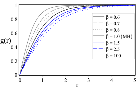
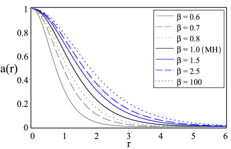
Figure 1: The Higgs profile $g(r)$ (upper) and the gauge field profile $a(r)$ (lower) for the model (39) with a $|\phi|^{4}$-self-dual-potential (29) and some values of $\beta>1/2$.

The behavior of $g(r)$ and $a(r)$ near the boundaries can be easily determined by solving the self-dual equations (62) and (63) around the boundary values (57) and (58). This way, near the origin, the profile functions behave as

$$g(r) \approx G_{n}^{{}^{(f_{{}_{4}})}}r^{\left|n\right|}+...,$$ (66)

$$a(r) \approx n\mp\frac{e^{2}v^{2}}{2}f_{{}_{4}}r^{2}+....$$ (67)

On the other hand, when $r\rightarrow\infty$ they behave as

$$g(r) \simeq 1-\frac{G_{\infty}^{{}^{(f_{{}_{4}})}}}{\sqrt{r}}e^{-m_{{}_{4}}r},$$ (68)

$$a(r) \simeq {m_{{}_{4}}}G_{\infty}^{{}^{(f_{{}_{4}})}}\sqrt{r}e^{-m_{{}_{4}}r}.$$ (69)

The constants $G_{n}^{{}^{(f_{{}_{4}})}}>0$ and $G_{\infty}^{{}^{(f_{{}_{4}})}}$ can be determined only numerically and $m_{{}_{4}}$ being the self-dual mass,

$$m_{{}_{4}}=m_{{}_{MH}}\sqrt{f_{{}_{4}}},$$ (70)

with $m_{{}_{MH}}=\sqrt{2}ev$ standing for the mass of the usual self-dual Maxwell-Higgs bosons.

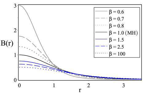
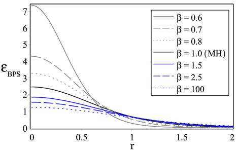
Figure 2: The magnetic field $B(r)$ (upper) and the BPS energy density $\varepsilon_{{}_{BPS}}(r)$ (lower) coming from the model (39) with a $|\phi|^{4}$-self-dual-potential (29) and some values of $\beta>1/2$.

We perform the numerical analysis of the $|\phi|^{4}$-models arising from the $k$-generalized model defined in Eq. (39), i.e., we consider the BPS equations (62) and (63) with

$$f^{(\beta)}_{{}_{4}}=\frac{\beta}{2\beta-1},$$ (71)

for some values of $\beta>1/2$.

In order to compute the numerical solutions we choose the upper signs, $e=v=1$ and the configurations with winding number $n=1$. The profiles for the Higgs and gauge fields are given in Fig. 1, the correspondent ones for the magnetic field and the self-dual energy density are depicted in Fig. 2.

A brief analysis of the amplitude (71) elucidates that, within the range $1/2<\beta<1$, the mass $m_{{}_{4}}$ increase for $\beta\rightarrow 1/2$, whilst reaching $m_{{}_{4}}\rightarrow m_{{}_{MH}}$ for $\beta\rightarrow 1$. On the other hand, for $\beta>1$, the mass $m_{{}_{4}}$ decreases continuously whenever $\beta$ increases attaining its minimum value $m_{{}_{4}}\rightarrow ev$ when $\beta\rightarrow\infty$. It explains the changes in the vortex-core size showed in the Figs. 1 and 2.

For $n=1$, the magnetic field and the BPS energy density attain their maximum amplitude at origin (see Fig. 2) and they are given by

$$B(0) = ev^{2}f^{(\beta)}_{{}_{4}},$$ (72)

$$\varepsilon_{{}_{BPS}}(0) = e^{2}v^{4}f^{(\beta)}_{{}_{4}}+2v^{2}(G_{1}^{{}^{(f_{{}_{4}})}})^{2},$$ (73)

respectively. The function (71) explains clearly because the amplitudes in relation to the MH ones ($\beta=1$) are higher for $1/2<\beta<1$ or smaller for $\beta>1$.

From the Eqs. (63), (70) and (65) we can establish the general conclusion for $|\phi|^{4}$-configurations when compared with the correspondent Maxwell-Higgs vortices: The $k$-generalization besides modifies the amplitude of magnetic field and the masses of the self-dual bosons also alters the self-dual energy density. The change in the boson mass value implies that the vortex-core size can be increased or diminished.

IV.2 Vortices in ${|\phi|^{6}}$-models

We have demonstrated that the Lagrangian density (3) also supports $|\phi|^{6}$-models whose self-dual equations are given by (20) together with (43) or (49). Such equations in the vortex Ansatz are written as

$$\frac{dg}{dr}=\pm\frac{ag}{r},$$ (74)

$$B=-\frac{1}{er}\frac{da}{dr}=\pm f_{{}_{6}}\frac{2e^{3}v^{4}}{\kappa^{2}}g^{2}(1-g^{2}),$$ (75)

where $f_{{}_{6}}>0$ (depending on $\beta$ or $\Delta$)  is given by

$$f_{{}_{6}}=\left\{\begin{array}[]{ccc}\displaystyle{\frac{\beta}{2\beta-1}}&,&\text{in Eq. (\ref{6m22}), }\\[9.95863pt] \displaystyle\frac{\Delta K_{Y}(\Delta)}{2\Delta K_{Y}(\Delta)+K(\Delta)}&,&\text{in Eq. (\ref{6m1-2}).}\end{array}\right.$$ (76)

The self-dual energy density is given by

$$\varepsilon_{sd}={2f_{{}_{6}}U_{{}_{CSH}}}+2v^{2}\left(\frac{ag}{r}\right)^{2}.$$ (77)

The profiles for $r\rightarrow 0$ behave as

$$g(r) \approx G_{n}^{{}^{(f_{{}_{6}})}}r^{\left|n\right|}+...,$$ (78)

$$a(r) \approx n\mp f_{{}_{6}}\frac{e^{4}v^{4}}{\kappa^{2}}\frac{\left(G_{n}^{{}^{(f_{{}_{6}})}}\right)^{2}}{\left(|n|+1\right)}r^{2|n|+2}+....$$ (79)

For $r\rightarrow\infty$, the asymptotic behavior is

$$g(r) \simeq 1-\frac{G_{\infty}^{{}^{(f_{{}_{6}})}}}{\sqrt{r}}e^{-m_{{}_{6}}r},$$ (80)

$$a(r) \simeq \frac{G_{\infty}^{{}^{(f_{{}_{6}})}}}{m_{{}_{6}}}\sqrt{r}e^{-m_{6}r}.$$ (81)

The constants $G_{n}^{{}^{(f_{{}_{6}})}}>0$ and $G_{\infty}^{{}^{(f_{{}_{6}})}}$ are determined numerically. The self-dual mass $m_{{}_{6}}$ is given by

$$m_{{}_{6}}=m_{{}_{CSH}}\sqrt{f_{{}_{6}}},$$ (82)

with $m_{{}_{CSH}}=2e^{2}v^{2}/\kappa$ standing for self-dual CSH mass.

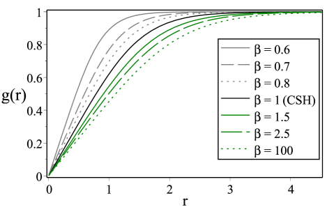
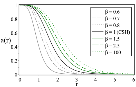
Figure 3: The profiles $g(r)$ (upper) and $a(r)$ (lower) coming from the model (39) with the $|\phi|^{6}$-self-dual-potential (37) and some values of $\beta>1/2$.

Similarly to the case of the $|\phi|^{4}$-models, we perform the numerical analysis of the $|\phi|^{6}$-models arising from the $k$-generalized model defined in Eq. (39). So, we consider the BPS equations (62) and (63) with $f^{(\beta)}_{{}_{6}}$ given by Eq. (71), i.e., $f^{(\beta)}_{{}_{6}}=\beta/(2\beta-1)$ . In order to compute the numerical solutions we choose the upper signs, $e=v=\kappa=1$ and the configurations with winding number $n=1$. The profiles for the Higgs and gauge fields are given in Fig. 3, the correspondent ones for the magnetic field and the self-dual energy density are depicted in Fig. 4.

The Figs. 3 and 4 shows the changes in the core-size of the vortex whenever the parameter $\beta$ changes its values. Such a effect has been also observed in the $|\phi|^{4}$-models analyzed previously.

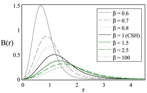
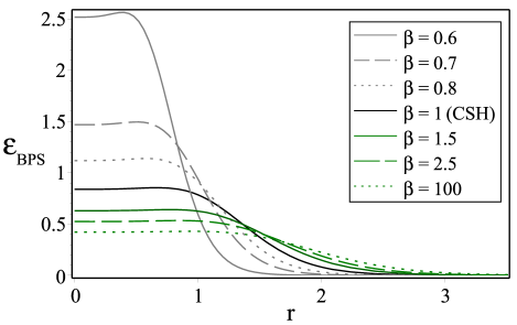
Figure 4: The magnetic field $B(r)$ (upper) and the BPS energy density $\varepsilon_{{}_{BPS}}(r)$ (lower) coming from the model (39) with the $|\phi|^{6}$-self-dual-potential (37) and some values of $\beta>1/2$.

For $n=1$, the magnetic field profiles are rings around the origin (see upper figure in Fig. 4) whose maximum amplitude is

$$B^{{}^{(\text{max})}}(r^{*})=\frac{e^{3}v^{4}}{2\kappa^{2}}\frac{\beta}{2\beta-1},$$ (83)

for a $r^{*}$ such that $g(r^{*})=\sqrt{2}/2$.

On the other hand, for $n=1$, the amplitude at origin of the BPS energy density is

$$\varepsilon_{{}_{BPS}}(0)=2v^{2}(G_{1}^{{}^{(f_{{}_{6}})}})^{2},$$ (84)

it changes whenever $\beta$ do it, i.e., the amplitudes in relation to $\beta=1$ ones are higher for $1/2<\beta<1$ or smaller for $\beta>1$ (see lower figure in Fig. 4).

IV.3 Delocalized self-dual vortices

In the previous examples we have studied localized vortex solutions whose behavior for very large values of $r$ is similar to the one of the Abrikosov-Nielsen-Olesen vortices, i.e., they have a exponential decay. Now we go to show that the $k$-generalized models defined by the Lagrangian density (3) can engender delocalized vortex, i.e., solutions possessing for $r\rightarrow\infty$ a power-law decay.

We present such solution by means of the model defined in Eq. (39) whose second BPS equation is given by Eq. (40). The delocalized vortices are obtained by choosing the following self-dual potential,

$$V_{sd}(g)=\frac{e^{2}v^{4}}{2}\left(1-g^{2}\right)^{2+2/\gamma}.$$ (85)

It is obtained from (41) by selecting appropriately the functions $h(g)$ and $\mathcal{U}(g)$. Here the parameter $\gamma>0$ will define the power-law decay ($r^{-\gamma}$) for large values of $r$ of the self-dual solutions.

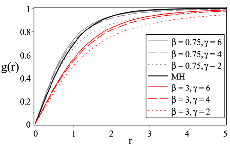
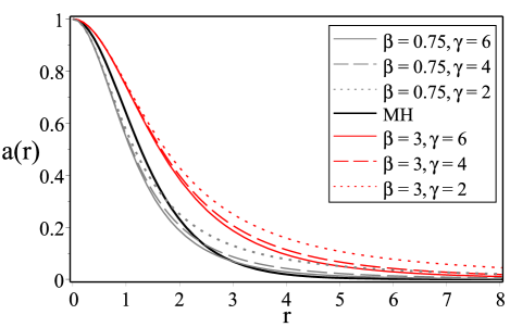
Figure 5: The profiles $g(r)$ (upper) and $a(r)$ (lower) coming from the model (39) with self-dual potential (85).

Then, the BPS equations describing the self-dual vortex solutions are

$$\frac{dg}{dr}=\pm\frac{ag}{r},$$ (86)

$$B=-\frac{1}{er}\frac{da}{dr}=\pm\frac{\beta}{2\beta-1}ev^{2}\left(1-g^{2}\right)^{1+2/\gamma}.$$ (87)

It is clear that the BPS equations of the usual Maxwell-Higgs model can be obtained when $\beta=1$ and $\gamma\rightarrow\infty$.

The positive-definite self-dual energy density is

$$\varepsilon_{{}_{BPS}}=\frac{2\beta}{2\beta-1}V_{sd}(g)+2v^{2}\left(\frac{ag}{r}\right)^{2}.$$ (88)

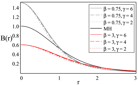
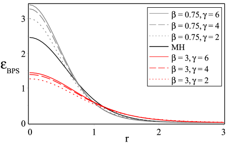
Figure 6: The magnetic field $B(r)$ (upper) and the BPS energy density $\varepsilon_{{}_{BPS}}(r)$ (lower) coming from the model (39) with self-dual potential (85).

The behavior of $g(r)$ and $a(r)$ when $r\rightarrow 0$ is obtained by solving the self-dual equations (86) and (87) around the boundary values (57). Such analysis gives

$$g(r) \approx G_{n}^{{}^{(\gamma)}}r^{\left|n\right|}+...,$$ (89)

$$a(r) \approx n\mp\frac{\beta}{2(2\beta-1)}\left(ev\right)^{2}r^{2}+.....$$ (90)

We see that the behavior is similar to the localized vortices previously analyzed.

On the other hand, the solution of the BPS equations (86) and (87) for $r\rightarrow\infty$ provides a power-law decay for the asymptotic behavior for the profiles $g(r)$ and $a(r)$,

$$g(r) \simeq 1-\frac{1}{2}\left(\frac{\gamma^{2}(2\beta-1)}{2\beta}\right)^{\gamma/2}\left(ev\right)^{-\gamma}\frac{1}{r^{\gamma}},$$ (91)

$$a(r) \simeq \frac{\gamma}{2}\left(\frac{\gamma^{2}(2\beta-1)}{2\beta}\right)^{\gamma/2}\left(ev\right)^{-\gamma}\frac{1}{r^{\gamma}}.$$ (92)

It means that the vortex solutions are delocalized configurations because their slow decay for long distances in contrast with the Abrikosov-Nielsen-Olesen vortices.

It is well know that the so-called London limit n013 provides the behavior of the fields of a vortex in the full Ginzburg-Landau model which is correctly predicts that the magnetic field varies monotonically and it is exponentially localized at large distances. However, there are vortex solutions having a delocalized magnetic field with profiles possessing slowly decaying. These delocalized vortices with power-law decay has been obtained by studying magnetic field delocalization in two-component superconductors Babaev . Recently, such a behavior has been also reported in diamagnetic vortices generated within of a Chern-Simons theory xxzz .

In order to compute the numerical solutions for the delocalized vortices, we have select the upper signs, $e=v=1$ and the configurations with winding number $n=1$. The numerical solutions of the BPS equations (86) and (87) have been performed for fixing $\beta=0.75$ (grey lines) and $\beta=3$ (red lines). For each $\beta$ we have selected some values of the power $\gamma=2,4,6$. The resulting profiles for the Higgs and gauge fields are given in Fig. 5, the correspondent ones for the magnetic field and the self-dual energy density are depicted in Fig. 6.

V Ending comments

We have shown the existence of self-dual configurations in Abelian-Higgs models where the kinetic term of gauge field is a highly nonlinear function of $F_{\mu\nu}F^{\mu\nu}$. Our study is based in the Lagrangian density (3) which in stationary regimen provides electrically neutral configurations. Starting from the canonical energy density, we have implemented consistently the BPS formalism by obtaining the general form of the self-interaction (potential) allowing to establish that the total energy has a lower bound proportional to the magnetic flux. Consequently, the field configurations having the minimum energy satisfy highly nonlinear first-order differential equations the so called self-dual or BPS equations. We have verified that the Lagrangian density (3) besides to support self-dual models in absence of a self-interacting potential also supports infinite twinlike models with $|\phi|^{4}$-potential or $|\phi|^{6}$-potential.

Among the infinite set of possible configurations, we have found families of $k$-generalized models whose self-dual equations have a form mathematically similar to the ones arising in the Maxwell-Higgs or Chern-Simons-Higgs models, i.e., $|D_{\pm}\phi|=0$ and $B=\pm\mathcal{V}(V_{sd}(|\phi|),h(|\phi|),{\cal{U}}(|\phi|)$, where $\mathcal{V}$ is some function of the self-dual potential and generalizing functions. The models with such a set of BPS equation could fulfill the condition (44) despite the self-dual potential (41) present a complicated form but by choosing suitably the generalizing functions it is able to describe $|\phi|^{4}$ or $|\phi|^{6}$ models. An example is the model defined by Eq. (39) with potential given by Eq. (46). Furthermore, in absence of a explicit SSB potential, the condition (50) allows to describe simplest $k$-generalized models admitting only $|\phi|^{4}$-self-interactions (see Eq. (53)).

With the aim to show explicitly that the BPS equations are able to provide well-behaved solutions, we have considered the model given by Eq. (39) to study axially symmetric vortices. For a self-dual potential type $|\phi|^{4}$ or $|\phi|^{6}$, we have shown that the $k$-generalized model is able to produce solutions that for long distances have a exponential decay (as Abrikosov-Nielsen-Olesen vortices). We have also shown that for the self-dual potential given by Eq. (85), the vortices for long distances have a power-law decay (characterizing delocalized vortices). They are remarkable solutions because such a behavior has been obtained by studying magnetic field delocalization in two-component superconductors Babaev and recently in diamagnetic vortices xxzz . In all cases, we have observed that the generalization modifies the vortex-core size, the magnetic field amplitude, the BPS energy density, the self-dual masses but the total energy remains proportional to the quantized magnetic flux.

Finally, we consider two interesting challenges: Firstly to study the influence of the $k$-generalized dynamics of the gauge field in the existence of charged self-dual configurations in Abelian Higgs models with Chern-Simons term or with Lorentz symmetry breaking terms. A second study is to analyze cosmic string solutions for gauge field with $k$-generalized dynamics in the context of modify gravity. Advances in this direction will be reported elsewhere.

- (1) N. Manton and P. Sutcliffe, Topological Solitons (Cambridge University Press, Cambridge, England, 2004).
- (2) D. Bazeia, E. da Hora, C. dos Santos and R. Menezes, Phys. Rev. D 81 (2010) 125014. D. Bazeia, E. da Hora, R. Menezes, H. P. de Oliveira and C. dos Santos, Phys. Rev. D 81 (2010) 125016. C. dos Santos and E. da Hora, Eur. Phys. J. C 70 (2010) 1145; Eur. Phys. J. C 71 (2011) 1519. C. dos Santos, Phys. Rev. D 82 (2010) 125009. D. Bazeia, E. da Hora and D. Rubiera-Garcia, Phys. Rev. D 84 (2011) 125005. C. dos Santos and D. Rubiera-Garcia, J. Phys. A 44 (2011) 425402. D. Bazeia, R. Casana, E. da Hora and R. Menezes, Phys. Rev. D 85 (2012) 125028. R. Casana, M. M. Ferreira Jr. and E. da Hora, Phys. Rev. D 86 (2012) 085034. R. Casana, M. M. Ferreira, E. da Hora and C. dos Santos, Phys. Lett. B 722 (2013) 193. D. Bazeia, R. Casana, M. M. Ferreira Jr., E. da Hora and L. Losano, Phys. Lett. B 727 (2013) 548. C. Adam, L. A. Ferreira, E. da Hora, A. Wereszczynski and W. J. Zakrzewski, J. High Energy Phys. 1308 (2013) 062. R. Casana, M. M. Ferreira Jr., E. da Hora and C. dos Santos, Adv. in High Energy Phys. 2014 (2014) 210929.
- (3) D. Bazeia, E. da Hora, C. dos Santos and R. Menezes, Eur. Phys. J. C 71 (2011) 1833
- (4) E. Babichev, Phys. Rev. D 74 (2006) 085004; Phys. Rev. D 77 (2008) 065021. C. Adam, N. Grandi, J. Sanchez-Guillen and A. Wereszczynski, J. Phys. A 41 (2008) 212004. C. Adam, J. Sanchez-Guillen and A. Wereszczynski, J. Phys. A 40 (2007) 13625; Phys. Rev. D 82 (2010) 085015. C. Adam, N. Grandi, P. Klimas, J. Sanchez-Guillen and A. Wereszczynski, J. Phys. A 41 (2008) 375401. C. Adam, P. Klimas, J. Sanchez-Guillen and A. Wereszczynski, J. Phys. A 42 (2009) 135401. C. Adam, J. M. Queiruga, J. Sanchez-Guillen and A. Wereszczynski, Phys. Rev. D 84 (2011) 025008; Phys. Rev. D 84 (2011) 065032. P. P. Avelino, D. Bazeia and R. Menezes, Eur. Phys. J. C 71 (2011) 1683. D. Bazeia and R. Menezes, Phys. Rev. D 84 (2011) 105018. C. Adam and J. M. Queiruga, Phys. Rev. D 85 (2012) 025019. C. Adam, C. Naya, J. Sanchez-Guillen and A. Wereszczynski, Phys. Rev. D 86 (2012) 085001; Phys. Rev. Dr 86 (2012) 045015. D. Bazeia, E. da Hora and R. Menezes, Phys. Rev. D 85 (2012) 045005. D. Bazeia, A. S. Lobão Jr. and R. Menezes, Phys. Rev. D 86 (2012) 125021.
- (5) M. Andrews, M. Lewandowski, M. Trodden, and D. Wesley, Phys. Rev. D 82, 105006 (2010).
- (6) C. Adam and J. M. Queiruga, Phys. Rev. D 84, 105028 (2011).
- (7) D. Bazeia, J. D. Dantas, A. R. Gomes, L. Losano, and R. Menezes, Phys. Rev. D 84, 045010 (2011).
- (8) D. Bazeia and R. Menezes, Phys. Rev. D 84, 125018 (2011).
- (9) C. Armendariz-Picon, T. Damour and V. Mukhanov, Phys. Lett. B 458 (1999) 209.
- (10) V. Mukhanov and A. Vikman, J. Cosmol. Astropart. Phys. 02 (2005) 004.
- (11) C. Armendariz-Picon and E. A. Lim, J. Cosmol. Astropart. Phys. 08 (2005) 007.
- (12) J. Garriga and V. Mukhanov, Phys. Lett. B 458 (1999) 219. R. J. Scherrer, Phys. Rev. Lett. 93 (2004) 011301.
- (13) M. Giovannini, Phys. Rev. D 66 (2002) 044016.
- (14) K. Shiraishi, S. Hirenzaki, Int. J. Mod. Phys. A 6 (1991) 2635.
- (15) R. Casana, E. da Hora, D. Rubiera-Garcia, C. dos Santos, Eur. Phys. J. C 75 (2015) 380.
- (16) A. Vilenkin, Phys. Rep. 121 (1985) 263. A. A. Starobinsky, Phys. Lett. 91B (1980) 99. S. M. Carroll, V. Duvvuri, M. Trodden and M. S. Turner, Phys. Rev. D 70 (2004) 043528. K. S. Stelle, Gen. Relativ. Grav., 9 (1978) 353. A. De Fellice, D. F. Mota and S. Tsujikawa, Phys. Rev. D 81 (2010) 023532.
- (17) M. Sakellariadou, Phys. Proc. Suppl. 68 (2009) 192.
- (18) E. Bogomol’nyi, Sov. J. Nucl. Phys. 24 (1976) 449 .
- (19) H. J. de Vega and F. A. Schaposnik, Phys. Rev. D 14 (1976) 1100.
- (20) J. Hong, Y. Kim and P. Y. Pac, Phys. Rev. Lett. 64 (1990) 2230.
- (21) R. Jackiw and E. J. Weinberg, Phys. Rev. Lett. 64 (1990) 2234; R. Jackiw, K. Lee and E. J. Weinberg, Phys. Rev. D. 42 (1990) 3488.
- (22) H. B. Nielsen and P. Olesen, Nucl. Phys. B 61 (1973) 45.
- (23) E. Babaev, Phys. Rev. Lett. 89, 067001 (2002).
- (24) E. Babaev, J. Jykk and M. Speight, Phys. Rev. Lett. 103 (2009) 237002.
- (25) Mohamed M. Anber, Yannis Burnier, Eray Sabancilar, and Mikhail Shaposhnikov, Phys. Rev. D 92, 085049 (2015).