Simple model of the slingshot effect

Abstract

We present a detailed quantitative description of the recently proposed “slingshot effect”. Namely, we determine a broad range of conditions under which the impact of a very short and intense laser pulse normally onto a low-density plasma (or matter locally completely ionized into a plasma by the pulse) causes the expulsion of a bunch of surface electrons in the direction opposite to the one of propagation of the pulse, and the detailed, ready-for-experiments features of the expelled electrons (energy spectrum, collimation, etc). The effect is due to the combined actions of the ponderomotive force and the huge longitudinal field arising from charge separation. Our predictions are based on estimating 3D corrections to a simple, yet powerful plane 2-fluid magnetohydrodynamic (MHD) model where the equations to be solved are reduced to a system of Hamilton equations in one dimension (or a collection of) which become autonomous after the pulse has overcome the electrons. Experimental tests seem to be at hand. If confirmed by the latter, the effect would provide a new extraction and acceleration mechanism for electrons, alternative to traditional radio-frequency-based or Laser-Wake-Field ones.

I Introduction and set-up

Laser-driven Plasma-based Acceleration (LPA) mechanisms were first conceived by Tajima and Dawson in 1979 Tajima-Dawson1979 and have been intensively studied since then. In particular, after the rapid development StriMou85 ; PerMou94 of chirped pulse amplification laser technology - making available compact sources of intense, high-power, ultrashort laser pulses - the Laser Wake Field Acceleration (LWFA) mechanism Tajima-Dawson1979 ; Gorbunov-Kirsanov1987 ; Sprangle1988 allows to generate extremely high acceleration gradients ($>$1GV/cm) by plasma waves involving huge charge density variations. Since 2004 experiments have shown that LWFA in the socalled bubble (or blowout) regime can produce electron bunches of high quality (i.e. very good collimation and small energy spread), energies of up to hundreds of MeVs ManEtAl04 ; GedEtAl04 ; FauEtAl04 or more recently even GeVs WanEtAl13 ; LeeEtAl14 . This allows a revolution in acceleration techniques of charged particles, with a host of potential applications in research (particle physics, materials science, structural biology, etc.) as well as applications in medicine, optycs, etc.

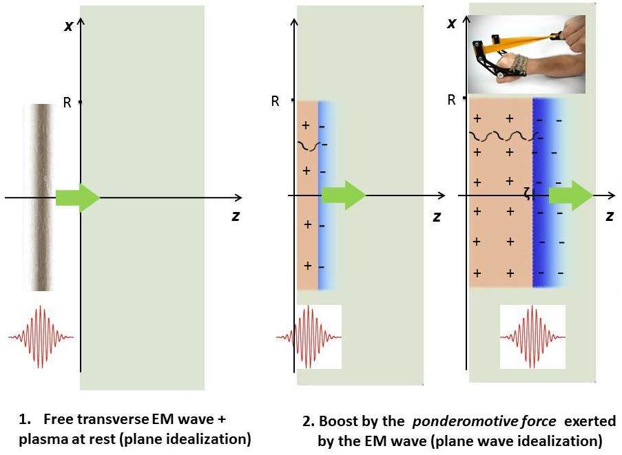
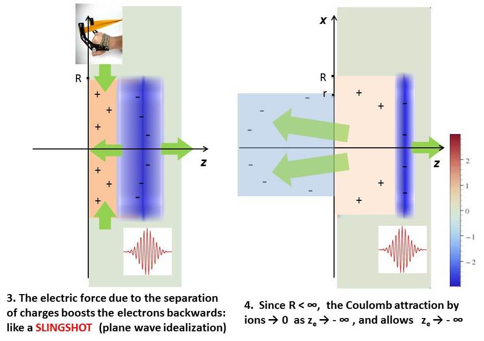
Figure 1: Schematic stages of the slingshot effect

In the LWFA and its variations the laser pulse travelling in the plasma leaves a wakefield of plasma waves behind; a bunch of electrons (either externally Irman2007 or self injected Joshi2006 ) can be accelerated “surfing” one of these plasma waves and exit the plasma sample just behind the pulse, in the same direction of propagation of the latter (forward expulsion). In Ref. FioFedDeA14 a new LPA mechanism, named slingshot effect, has been proposed, in which a bunch of electrons is expected to be accelerated and expelled backwards from a low-density plasma sample shortly after the impact of a suitable ultra-short and ultra-intense laser pulse in the form of a pancake normally onto the plasma (see fig. 1). The surface electrons (i.e. plasma electrons in a thin layer just beyond the vacuum-plasma interface) first are all displaced forward (with respect to the ions) by the ponderomotive force $F\!_{p}\!:=\!\langle-e(\frac{{\bm{v}}}{c}\times{\bm{B}})^{z}\rangle$ generated by the pulse, leaving a layer of ions completely depleted of electrons (here $\langle\>\rangle$ is the average over a period of the laser carrier wave, ${\bm{E}},{\bm{B}}$ are the electric and magnetic fields, ${\bm{v}}$ is the electron velocity, $c$ is the speed of light, $\hat{\bm{z}}$ is the direction of propagation of the laser pulse); $F\!_{p}$ is positive (negative) while the modulating amplitude $\epsilon_{s}$ of the pulse respectively grows (decreases). These electrons are then pulled back by the longitudinal electric force $F_{e}^{z}\!=\!-eE^{z}$ exerted by the ions and the other electrons, and leave the plasma. [In the meanwhile the pulse proceeds deeper into the plasma, generating a wakefield.] Tuning the electron density in the range where the plasma oscillation period $T\!_{{\scriptscriptstyle H}}$footnote1 is about twice the pulse duration $\tau$, we can make these electrons invert their motion when they are reached by the maximum of $\epsilon_{s}$, so that the negative part of $F\!_{p}$ (due to the subsequent decrease of $\epsilon_{s}$) adds to $F_{e}^{z}$ in accelerating them backwards; thus the total work $W\!=\!\int_{0}^{\tau}\!dt\,F\!_{p}\langle v^{z}\rangle$ done by the ponderomotive force is maximal footnote2 . Provided the laser spot size $R$ is sufficiently small a significant part of the expelled electrons will have enough energy to win the attraction by ions and escape to infinity.

Very short $\tau$’s and huge nonlinearities make approximation schemes based on Fourier analysis and related methods (slowly varying amplitude approximation, frequency-dependent refractive indices,…) unconvenient. On the contrary, in the relevant space-time region a MHD description of the impact is self-consistent, simple and predictive (collisions are negligible, and recourse to kinetic theory is not needed). Here we develop and improve the 2-fluid MHD approach introduced in FioFedDeA14 ; Fio14JPA and apply it to determine a broad range of conditions enabling the effect, as well as detailed quantitative predictions about it (a brief summary is given in FioDeN16 ; Fio16b ). In section II we study the plane problem ($R\!=\!\infty$) and show that for sufficiently low density and small times (after the impact) we can neglect the radiative corrections [back-reaction of the plasma on the electromagnetic (EM) field (3)] and determine the motion of the surface electrons in the bulk by (numerically) solving a single system of two coupled first order ordinary differential equations of Hamiltonian form, if the initial density $\widetilde{n_{0}}$ is step-shaped, or a collection of such systems, otherwise; the role of ‘time’ is played by the light-like coordinate $\xi\!=\!ct-z$. The rough model of FioFedDeA14 considered only step-shaped $\widetilde{n_{0}}$ and was based on neglecting: $F_{e}^{z}$ during the forward motion, $F_{p}$ during the backward motion of the electrons; the estimates could be considered reliable only for very low, unrealistic $\widetilde{n_{0}}$. Here $\widetilde{n_{0}}$ needs no longer to be so low, nor step-shaped, as in FioFedDeA14 , because we take $F_{e}^{z},F_{p}$ in due account during the whole motion of the electrons. In section III we heuristically modify the potential energy outside the bulk to account for finite $R$ and determine a $R$-range such that the motion of the surface electrons coming from some inner cylinder $\rho^{2}\!\leq\!r^{2}\!<\!R^{2}$ be (by causality) well approximated by the solution of the correspondingly modified Hamilton equations; we then find which electrons indeed escape to infinity and estimate in detail their final energy spectrum, collimation, total number, charge and energy. To be specific, in section IV we specialize predictions to potential experiments at the FLAME facility (LNF, Frascati) or the ILIL laboratory (INO-CNR, Pisa). We welcome 3D simulations and experiments checking these predictions; the experimental conditions are at hand in many laboratories. In section V we discuss the results, the conditions for their validity and draw the conclusions.

As a context remark, we recall that relatively simple 2-fluid magnetohydrodynamic models can be used also to describe the complicated physics of the impact of very intense and short laser pulses on overdense solid targets. If the density gradient of the target is sufficiently steep, the massive displacement of electrons (induced by the ponderomotive force) with respect to ions (named snowplow in SahEtAl13 ; Sah14 ) produces a longitudinal electric force which may accelerate also protons or other light ions, either backward or forward, by the socalled Skin-Layer Ponderomotive Acceleration BadEtAl04 or Relativistically Induced Transparency Acceleration SahEtAl13 ; Sah14 mechanisms.

The 2-fluid magnetohydrodynamic framework

The set-up is as follows. We assume that the plasma is initially neutral, unmagnetized and at rest with electron (and proton) density equal to zero in the region  $z\!<\!0$. We describe the plasma as consisting of a static background fluid of ions (the motion of ions can be neglected during the short time interval in which the effect occurs) and a fully relativistic collisionless fluid of electrons, with the “plasma + EM field” system fulfilling the Lorentz-Maxwell and the continuity equations. We show a posteriori that such a MHD treatment is self-consistent in the spacetime region of interest. We denote as  ${\bm{x}}_{e}(t,{\bm{X}})$  the position at time $t$ of the electrons’ fluid element initially located at ${\bm{X}}\!\equiv\!(X,Y,Z)$, and for each fixed $t$ as ${\bm{X}}_{e}(t,{\bm{x}})$ the inverse map [${\bm{x}}\!\equiv\!(x,y,z)$]. For brevity, we refer: to such a fluid element as to the “${\bm{X}}$ electrons”; to the fluid elements with arbitrary $X,Y$ and specified $Z$, or with ${\bm{X}}$ in a specified region $\Omega$, respectively as the “$Z$ electrons” or the “$\Omega$ electrons”. We denote as $m,n_{e},{\bm{v}}_{e}$ the electron mass, Eulerian density and velocity and often use the dimensionless fields  ${\bm{\beta}}_{e}\!\equiv\!{\bm{v}}_{e}/c$, ${\bm{u}}_{e}\!\equiv\!{\bm{p}}_{e}/mc\!=\!{\bm{\beta}}_{e}/\sqrt{1\!-\!{\bm{\beta}}_{e}^{2}}$, $\gamma_{e}\!\equiv\!1/\sqrt{1\!-\!{\bm{\beta}}_{e}^{2}}\!=\!\sqrt{1\!+\!{\bm{u}}_{e}^{2}}$.  The equations of motion are

$$\begin{array}[]{l}\displaystyle\frac{d{\bm{p}}_{e}}{dt}\!=\!-e\left({\bm{E}}\!+\!\frac{{\bm{v}}_{e}}{c}\wedge{\bm{B}}\right),\\[10.0pt] \partial_{t}{\bm{x}}_{e}(t,{\bm{X}})={\bm{v}}_{e}\!\left[t,{\bm{x}}_{e}(t,{\bm{X}})\right]\end{array}$$ (1)

in CGS units ($d/dt\!\equiv\!\partial_{t}\!+\!{\bm{v}}_{e}\!\cdot\!\nabla_{x}$ is the electrons’ material derivative) and the initial conditions are ${\bm{p}}_{e}(0,{\bm{X}})\!=\!{\bf 0}$, ${\bm{x}}_{e}(0,{\bm{X}})\!=\!{\bm{X}}$ for $Z\!\geq\!0$. The Lagrangian fields depend on $t,{\bm{X}}$, rather than on $t,{\bm{x}}$, and are distinguished by a tilde, e.g. $\widetilde{n_{e}}(t,\!{\bm{X}})=n_{e}[t,\!{\bm{x}}_{e}(t,\!{\bm{X}})]$. The continuity equation $dn_{e}/dt\!+\!n_{e}\nabla_{x}\!\cdot{\bm{v}}_{e}=0$  follows from the local conservation of the number of electrons, which amounts to

$$\tilde{n}_{e}(t,{\bm{X}})\,\det\!\left(\frac{\partial{\bm{x}}_{e}}{\partial{\bm{X}}}\right)=\widetilde{n_{0}}({\bm{X}})\equiv\tilde{n}_{e}(0,{\bm{X}}).$$ (2)

We assume that $\widetilde{n_{0}}$ is independent of $X,Y$ and, as said, vanishes if $Z\!<\!0$; also as a warm-up to more general $Z$-dependence, we start by studying the case that it is constant in the region $Z\!\geq\!0$: $\widetilde{n_{0}}(Z)\!=\!n_{0}\theta(Z)$, where $\theta$ is the Heaviside step function. We consider a purely transverse EM pulse in the form of a pancake with cylindrical symmetry around the $z$-axis, propagating in the positive ${\hat{\bm{z}}}$ direction and hitting the plasma surface  $z\!=\!0$ at $t\!=\!0$. We schematize the pulse as a free plane pulse multiplied by a “cutoff” function $\chi\!_{{\scriptscriptstyle R}}(\rho)$ which is approximately equal to 1 for $\rho\!\equiv\sqrt{\!x^{2}\!+\!y^{2}}\!\leq\!R$ and rapidly goes to zero for $\rho\!>\!R$ (with some finite radius $R$, see fig. 1-1)

$${\bm{E}}^{{\scriptscriptstyle\perp}}\!(t,\!{\bm{x}})={\bm{\epsilon}}\!^{{\scriptscriptstyle\perp}}\!(ct\!-\!z)\,\chi\!_{{\scriptscriptstyle R}}(\rho),\qquad{\bm{B}}^{{\scriptscriptstyle\perp}}={\hat{\bm{z}}}\!\times\!{\bm{E}}\!^{{\scriptscriptstyle\perp}}$$ (3)

[in particular we consider $\chi\!_{{\scriptscriptstyle R}}(\rho)\!\equiv\!\theta(R\!-\!\rho)$]; the ‘pump’ ${\bm{\epsilon}}^{{\scriptscriptstyle\perp}}\!(\xi)$ vanishes outside some finite interval $0\!<\!\xi\!<\!l$ footnote2bis .

II Plane wave idealization

In the plane problem ($R\!=\!\infty$) the invertibility of ${\bm{x}}_{e}\!:\!{\bm{X}}\!\mapsto\!{\bm{x}}$ for all fixed $t$ amounts to $z_{e}(t\!,Z)$ being strictly increasing with respect to $Z$ for all $t$. Eq. (2) becomes

$$\begin{array}[]{l}\left[\tilde{n}_{e}\frac{\partial z_{e}}{\partial Z}\!\right]\!\!(t,\!Z)\!=\!\widetilde{n_{0}}(Z)\quad\Leftrightarrow\quad n_{e}(t,\!z)\!=\!\widetilde{n_{0}}\!\left[Z_{e}\!(\!t,\!z\!)\right]\frac{\partial Z_{e}}{\partial z}(t,\!z).\end{array}$$ (4)

Regarding ions as immobile, the Maxwell equations imply Fio14JPA that the longitudinal component of the electric field is related to $\widetilde{N}(Z)\!\equiv\!\int^{Z}_{0}\!dZ^{\prime}\,\widetilde{n_{0}}(Z^{\prime})$ (the number of electrons per unit surface in the layer $0\!\leq\!Z^{\prime}\!\leq\!Z$) by

$$E^{z}(t,z)\!=\!4\pi e\big{\{}\widetilde{N}(z)\!-\!\widetilde{N}[Z_{e}(t,z)]\big{\}}.\quad{}$$ (5)

We partially fix the gauge Fio14JPA imposing that the transverse (with respect to ${\hat{\bm{z}}}$) vector potential itself is independent of $x,y$, and hence is the physical observable ${\bm{A}}\!^{{\scriptscriptstyle\perp}}\!(t,z)\!=\!-\!\int^{t}_{-\!\infty}\!\!dt^{\prime}c{\bm{E}}^{{\scriptscriptstyle\perp}}\!(t^{\prime}\!,z)$; then  $c{\bm{E}}^{{\scriptscriptstyle\perp}}\!=\!-\partial_{t}{\bm{A}}\!^{{\scriptscriptstyle\perp}}$,  ${\bm{B}}\!=\!{\bm{B}}^{{\scriptscriptstyle\perp}}\!=\!{\hat{\bm{z}}}\!\wedge\!\partial_{z}{\bm{A}}\!^{{\scriptscriptstyle\perp}}$. As known, the transverse component of the Lorentz equation (1)₁ implies  ${\bm{p}}_{e}^{{\scriptscriptstyle\perp}}\!-\!\frac{e}{c}{\bm{A}}^{{\scriptscriptstyle\perp}}\!\!\!=$const on the trajectory of each electron;  this is zero at $t\!=\!0$,   hence  ${\bm{p}}_{e}^{{\scriptscriptstyle\perp}}\!=\!mc{\bm{u}}_{e}^{{\scriptscriptstyle\perp}}\!=\!e{\bm{A}}\!^{{\scriptscriptstyle\perp}}\!/c$. Hence ${\bm{u}}{}_{e}^{{\scriptscriptstyle\perp}}$ is determined in terms of ${\bm{A}}\!^{{\scriptscriptstyle\perp}}$. As in Fio14JPA , we introduce the positive-definite field

$$s_{e}\!\equiv\!\gamma_{e}\!-\!u^{z}_{e},$$ (6)

which we name electron s-factor.  $u_{e}^{z},\gamma_{e},{\bm{\beta}}_{e}^{{\scriptscriptstyle\perp}},\beta_{e}^{z}$ are recovered from ${\bm{u}}_{e}^{{\scriptscriptstyle\perp}},s_{e}$ through the formulae (44) of Fio14JPA :

$$\gamma_{e}\!=\!\frac{1\!+\!{\bm{u}}_{e}^{{\scriptscriptstyle\perp}}{}^{2}\!\!+\!s_{e}^{2}}{2s_{e}},\quad\>u_{e}^{z}\!=\!\frac{1\!+\!{\bm{u}}_{e}^{{\scriptscriptstyle\perp}}{}^{2}\!\!-\!s_{e}^{2}}{2s_{e}},\quad\>\displaystyle{\bm{\beta}}_{e}\!=\!\frac{{\bm{u}}_{e}}{\gamma_{e}}.\quad$$ (7)

Remarkably, all of (7) are rational functions of ${\bm{u}}_{e}^{{\scriptscriptstyle\perp}},s_{e}$ (no square roots appear). Moreover, fast oscillations of ${\bm{u}}_{e}^{{\scriptscriptstyle\perp}}$ affect $\gamma_{e},u_{e}^{z}$ but not $s_{e}$ [see the comments after (17)]. For these reasons it is convenient to use ${\bm{u}}_{e}^{{\scriptscriptstyle\perp}},s_{e}$ instead of ${\bm{u}}_{e}^{{\scriptscriptstyle\perp}},u_{e}^{z}$ as independent unknowns. The evolution equation of $s_{e}$ (difference of the ones of $\gamma_{e},u_{e}^{z}$; the former is the scalar product of (1)₁ with ${\bm{p}}_{e}/\gamma_{e}m^{2}c^{2}$) reads

$$\gamma_{e}\frac{ds_{e}}{dt}\!=\!\frac{eE^{{\scriptscriptstyle z}}}{mc}s_{e}\!+\!(\partial_{t}\!+\!c\partial_{z}){\bm{u}}_{e}^{{\scriptscriptstyle\perp}}{}^{2}.$$ (8)

The Maxwell equation for ${\bm{A}}\!^{{\scriptscriptstyle\perp}}$ takes the form  $(\partial_{0}^{2}\!-\!\partial_{z}^{2}){\bm{A}}\!^{{\scriptscriptstyle\perp}}\!+\!{\bm{A}}\!^{{\scriptscriptstyle\perp}}4\pi e^{2}n_{e}/mc^{2}\gamma_{e}\!=\!0$;  eq. (3) with $R\!=\!\infty$ implies ${\bm{A}}\!^{{\scriptscriptstyle\perp}}(t\!,z)\!=\!{\bm{\alpha}}\!^{{\scriptscriptstyle\perp}}(ct\!-\!z)$ for $t\!\leq\!0$, where ${\bm{\alpha}}^{{\scriptscriptstyle\perp}}\!(\xi)\!\equiv\!-\!\!\int^{\xi}_{-\infty}\!\!d\xi^{\prime}{\bm{\epsilon}}^{{\scriptscriptstyle\perp}}\!(\xi^{\prime})$. Using the Green function of the D’Alembertian $\partial_{0}^{2}\!-\!\partial_{z}^{2}$, abbreviating $x\!\equiv\!(t,z)$, these equations can be equivalently reformulated as the integral equation (42) of Fio14JPA

$${\bm{A}}\!^{{\scriptscriptstyle\perp}}(t\!,z)-{\bm{\alpha}}\!^{{\scriptscriptstyle\perp}}(ct\!-\!z)=-\!\!\displaystyle\int_{D\!_{x}\cap T}\!\!\!\!\!\!dt^{\prime}dz^{\prime}\left[\frac{2\pi e^{2}n_{e}}{mc\gamma_{e}}{\bm{A}}\!^{{\scriptscriptstyle\perp}}\right]\!\!(x^{\prime})\qquad$$ (9)

$$D\!_{x}\!\equiv\!\{(t^{\prime},z^{\prime})\>|\>{t}^{\prime}\!\leq\!t,\,|z\!-\!z^{\prime}|\!\leq\!{ct}\!-\!{ct}^{\prime}\},\quad T\!\equiv\!\{x\>|\>|z|\!<\!ct\}$$

The past, future causal cones $D\!_{x},T$, the supports of ${\bm{A}}^{{\scriptscriptstyle\perp}},\widetilde{n_{0}}(z)$, and their intersections are shown in fig. 2. For $t\!<\!0$  $D\!_{x}\!\cap\!T$  is empty, and the right-hand side of (9)₁ is zero, as it must be. Below we shall analyze the consequences of neglecting it also for small $t$, and determine the range of validity of such an approximation.

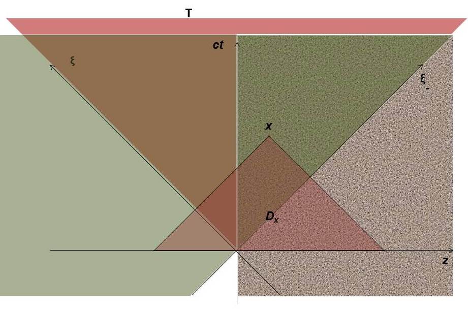
Figure 2: Past (light brown) and future (purple) causal cones $D\!_{x},T$; supports of ${\bm{A}}^{{\scriptscriptstyle\perp}}$ (light green) and $\widetilde{n_{0}}(z)$ (anthracite).

II.1 Motion of the electrons

$$\begin{array}[]{l}\mbox{Let}\qquad\displaystyle\hat{\bm{u}}^{{\scriptscriptstyle\perp}}(\xi)\!\equiv\!e{\bm{\alpha}}^{{\scriptscriptstyle\perp}}(\xi)/mc^{2},\qquad v(\xi)\!\equiv\!\hat{\bm{u}}^{{\scriptscriptstyle\perp}2}(\xi),\\[6.0pt] \qquad\quad\>\>F_{e}^{z}(z,\!Z)\!\equiv\!-4\pi e^{2}\left\{\widetilde{N}(z)\!-\!\widetilde{N}(Z)\right\}.\end{array}$$ (12)

$\widetilde{F_{e}^{z}}(t,\!Z)\!\equiv\!F_{e}^{z}[z_{e}\!(t,\!Z),\!Z]$ is the longitudinal electric force acting on the $Z$ electrons at time $t$; it is conservative, as it depends on $t$ only through $z_{e}(t,\!Z)$. The approximation ${\bm{A}}\!^{{\scriptscriptstyle\perp}}(t\!,z)\!=\!{\bm{\alpha}}\!^{{\scriptscriptstyle\perp}}(ct\!-\!z)$ implies ${\bm{u}}_{e}^{{\scriptscriptstyle\perp}}(t\!,z)\!=\!\hat{\bm{u}}^{{\scriptscriptstyle\perp}}(ct\!-\!z)$, and the last term of (8) vanishes. Replacing (5) in the Lagrangian version of (8),  we find for each $Z\!\geq\!0$ the equation   $\tilde{\gamma}_{e}\partial_{t}\tilde{s}_{e}=-\tilde{s}_{e}\widetilde{F_{e}^{z}}/mc$. The initial condition is $\tilde{s}_{e}(0,Z)\!\equiv\!1$. The other equation to be solved is (1)₂  with the initial condition  ${\bm{x}}_{e}(0,{\bm{X}})\!=\!{\bm{X}}$. By (7) one is thus led to the Cauchy problems (parametrized by $Z\!\geq\!0$)

$$\partial_{t}\frac{z_{e}\!-\!Z}{c}=\frac{1\!+\!v[ct\!-\!z_{e}(t,\!Z)]\!\!-\!\tilde{s}_{e}^{2}}{1\!+\!v[ct\!-\!z_{e}(t,\!Z)]\!+\!\tilde{s}_{e}^{2}},\quad\partial_{t}\tilde{s}_{e}=\displaystyle\frac{-\tilde{s}_{e}\!}{\tilde{\gamma}_{e}mc}\widetilde{F_{e}^{z}},\qquad$$ (13)

$$\>z_{e}(0,Z)\!-\!Z\!=\!0,\qquad\qquad\tilde{s}_{e}(0,Z)\!=\!1.\qquad\qquad\qquad\qquad$$ (14)

${\bm{x}}_{e}^{{\scriptscriptstyle\perp}}(t,\!{\bm{X}})$ is obtained from the solutions of (13-14) using (1), (7):

$${\bm{x}}^{{\scriptscriptstyle\perp}}_{e}(t,\!{\bm{X}})={\bm{X}}^{{\scriptscriptstyle\perp}}\!+\!\!\displaystyle\int^{t}_{0}\!\!dt{}^{\prime}\,c{\bm{\beta}}_{e}^{{\scriptscriptstyle\perp}}[t{}^{\prime},z_{e}(t{}^{\prime}\!,\!Z)].\qquad$$ (15)

For all fixed $Z$ the map $t\mapsto\tilde{\xi}(t,\!Z)\!\equiv\!ct\!-\!z_{e}(t\!,\!Z)$ is invertible, because the speed of electrons is always smaller than $c$. We can simplify (13) by the change of variables $(t,\!Z)\mapsto\big{(}\xi,Z\big{)}$, making the argument of $v$ an independent variable. Denoting the dependence on $\big{(}\xi,Z\big{)}$ by a caret [e.g. $\hat{s}(\xi,\!Z)\!=\!\tilde{s}_{e}(t,\!Z)$] and introducing the displacement from the initial position  $\hat{\Delta}(\xi,\!Z)\!\equiv\!\hat{z}_{e}(\xi,\!Z)\!-\!Z$,  we find  $\partial_{\xi}=(\tilde{\gamma}_{e}/c\,\tilde{s}_{e})\partial_{t}$, and (13) becomes

$$\hat{\Delta}^{\prime}=\displaystyle\frac{1\!+\!v}{2\hat{s}^{2}}\!-\!\frac{1}{2},\qquad\hat{s}^{\prime}=\frac{4\pi e^{2}}{mc^{2}}\left\{\!\widetilde{N}[\hat{\Delta}\!+\!Z]\!-\!\widetilde{N}(Z)\!\right\}\quad$$ (16)

(the prime means differentiation with respect to $\xi$). For $\xi\!\leq\!0$  $v(\xi)\!\equiv\!0$, $\hat{\Delta},\hat{s}$ remain constant, and we can replace the initial conditions $\hat{\Delta}(-Z,\!Z)\!=\!0$, $\hat{s}(-Z,\!Z)\!=\!1$ by

$$\>\hat{\Delta}(0,\!Z)\!=\!0,\qquad\qquad\hat{s}(0,\!Z)\!=\!1.\qquad\qquad\qquad\qquad$$ (17)

An alternative derivation of (16-17) with a deeper insight on the role of the $s$-factor is given in Fio16c . In the zero density limit $\widetilde{N}(Z)\!\equiv\!0$, $\hat{s}\!\equiv\!1$, (16-17) is integrable, and all unknowns are determined explicitly from ${\bm{\epsilon}}^{{\scriptscriptstyle\perp}}$ Fio14JPA ; Fio14 ). As $v\!\geq\!0$, even if ${\bm{\epsilon}}^{{\scriptscriptstyle\perp}}\!,{\bm{u}}^{{\scriptscriptstyle\perp}}\!,v$ oscillate fast with $\xi$, integrating (16) makes relative oscillations of $\hat{\Delta}$ much smaller than those of $v$ and those of $\hat{s}$ much smaller than the former; hence, $\hat{s}$ is practically smooth, see e.g. fig. 7. Setting  $q\!\equiv\!\hat{\Delta}$, $p\!\equiv\!-\hat{s}$,   for each fixed $Z$ (16) are the Hamilton equations (with ‘time’ $\xi$) $q^{\prime}=\partial\check{H}/\partial p$, $p^{\prime}=-\partial\check{H}/\partial q$ of a system with Hamiltonian $\check{H}(q,p,\xi;Z)\!\equiv\!H(q,-p,\xi;Z)$,

$$\begin{array}[]{l}H\!(\Delta,\!s,\!\xi;\!Z)\equiv\gamma(s,\xi)+{\cal U}(\Delta;\!Z),\quad\gamma(s,\xi)\!\equiv\!\displaystyle\frac{s^{2}\!\!+\!1\!+\!v(\xi)}{2s},\\[8.0pt] {\cal U}(\Delta;\!Z)\!\equiv\!\frac{4\pi e^{2}}{mc^{2}}\left[\widetilde{{\cal N}}\!(Z\!+\!\Delta)\!-\!\widetilde{{\cal N}}\!(Z)\!-\!\widetilde{N}\!(Z)\Delta\right],\\[8.0pt] \widetilde{{\cal N}}(Z)\equiv\int^{Z}_{0}\!\!\!dZ^{\prime}\,\widetilde{N}(Z^{\prime})\!=\!\int^{Z}_{0}\!\!\!dZ^{\prime}\,\widetilde{n_{0}}(Z^{\prime})\,(Z\!-\!Z^{\prime}).\end{array}$$ (21)

Defining ${\cal U}$ we have fixed the free additive constant so that ${\cal U}(0,\!Z)\!\equiv\!0$ for each $Z$;  $H\!-\!\sqrt{1\!+\!v}$  is positive definite. Below we shall abbreviate  $P(\xi;Z)\!\equiv\!\big{(}\hat{\Delta}(\xi;Z),\hat{s}(\xi;Z)\big{)}$.

The right-hand side of (16)₂ is an increasing function of $\hat{\Delta}$, because so is $\widetilde{N}(Z)$. As $v(\xi)$  is zero for $\xi\!\leq\!0$ and positive for small $\xi\!>\!0$, then so are also $\hat{\Delta}(\xi,\!Z)$ and $\hat{s}(\xi,\!Z)\!-\!1$.   Both keep increasing until $\hat{\Delta}$ reaches a positive maximum $\hat{\Delta}(\bar{\xi},Z)$ at the $\xi\!=\!\bar{\xi}(Z)\!>\!0$ such that

$$\hat{\Delta}^{\prime}(\bar{\xi},Z)=0\quad\Leftrightarrow\quad\hat{s}^{2}(\bar{\xi},\!Z)\!=\!1\!+\!v(\bar{\xi})$$ (22)

(note that $\bar{\xi}\!<\!l$ if $v(l)\!=\!0$). We shall denote as $\zeta\!\equiv\!\hat{\Delta}[\bar{\xi}(0),0]$ the maximum penetration of the $Z\!=\!0$ electrons. For $\xi\!>\!\bar{\xi}(Z)$ $\hat{\Delta}$ starts decreasing; $\hat{s}$ reaches a maximum at the $\xi\!=\!\xi_{r}(Z)$ such that $\hat{\Delta}(\xi_{r},\!Z)\!=\!0$ (i.e. at $\xi\!=\!\xi_{r}(Z)$ the $Z$ electrons have regained their initial $z$). Both decrease for $\xi\!>\!\xi_{r}(Z)$, until $\hat{s}$ becomes so small, and the right-hand side of (16)₁ so large, that first $\hat{\Delta}$, and then $\hat{s}\!-\!1$, are forced to abruptly grow again to positive values. This prevents $\hat{s}$ to vanish anywhere, consistently with (6). In $\xi$-intervals where $v(\xi)\!\equiv\!v_{c}\!\equiv$const, $H$ is conserved, and all trajectories $P(\xi;Z)$ in phase space (paths) are level curves $H(\Delta,s;Z)\!=\!h(Z)$, above the line $s\!=\!0$, integrable by quadrature Fio16 . For $Z\!=\!0$ the paths are unbounded with $\hat{\Delta}(\xi,0)\!\to\!-\infty$ as $\xi\!\to\!\infty$. For $Z\!>\!0$ the paths are cycles around the only critical point $C\!\equiv\!(\Delta,s)\!=\!(0,\sqrt{1\!+\!v_{c}})$ (a center); therefore for $\xi\!\geq\!l$ $v(\xi)\!=\!v(l)$, and these solutions are periodic. There exists a $Z_{b}\!>\!0$ such that: the paths $P(\xi;Z)$ with $Z\!<\!Z_{b}$ cross the $\hat{\Delta}\!=\!-Z$ line twice, i.e. go out of the bulk and then come back into it; the path $P(\xi;Z_{b})$ is tangent to this line in the point $(\hat{\Delta},\hat{s})\!=\!(-Z_{b},\sqrt{1\!+\!v(l)})$ (where $\hat{\Delta}^{\prime}\!=\!0$); the paths $P(\xi;Z)$ with $Z\!>\!Z_{b}$ do not cross this line. For $Z\!\leq\!Z_{b}$ let $\xi_{ex}(Z)$ be the first positive solution of the equation  $\hat{\Delta}(\xi,\!Z)\!=\!-Z$, i.e. at $\xi\!=\!\xi_{ex}(Z)$ the $Z$ electrons exit the bulk:

$$\hat{z}_{e}\left[\xi_{ex}(Z),\!Z\right]=0.$$ (23)

The function $\xi_{ex}(Z)$ is strictly increasing if $\partial_{{\scriptscriptstyle Z}}\hat{z}_{e}\!>\!0$.

For any family $P(\xi;Z)$ of solutions of (16-17) let

$$\hat{u}^{z}\!\equiv\!\displaystyle\frac{1\!+\!v\!-\!\hat{s}^{2}}{2\hat{s}},\qquad\qquad\hat{\gamma}\!\equiv\!\displaystyle\frac{1\!+\!v\!+\!\hat{s}^{2}}{2\hat{s}},$$

$$\hat{\bm{x}}_{e}(\xi,\!{\bm{X}})={\bm{X}}+\hat{\bm{Y}}\!(\xi,\!Z),\qquad\hat{\bm{Y}}\!(\xi,\!Z)\!\equiv\!\!\displaystyle\int\limits^{\xi}_{0}\!\!\!dy\,\frac{\hat{\bm{u}}(y,\!Z)}{\hat{s}(y,\!Z)},\qquad$$ (24)

$$c\hat{t}(\xi,Z)\!=\!Z\!+\!\hat{\Xi}(\xi,\!Z),\quad\hat{\Xi}(\xi,\!Z)\!\equiv\!\!\displaystyle\int^{\xi}_{0}\!\!\!\!\!dy\,\frac{\hat{\gamma}(y,\!Z)}{\hat{s}(y,\!Z)}\!=\!\xi\!+\!\hat{\Delta}(\xi,\!Z)$$

(note that $\hat{Y}^{z}\!=\!\hat{\Delta}$). The so defined $\hat{\bm{u}},\hat{\gamma},\hat{\bm{x}}_{e}$ are the solutions - expressed as functions of $\xi,{\bm{X}}$ - of all equations and initial conditions footnote3 . Note that $\hat{\bm{x}}_{e},\hat{t}$ can be obtained also solving the system of functional equations

$$\xi=ct\!-\!z,\qquad\hat{\Xi}(ct\!-\!z,\!Z)\!=\!ct\!-\!Z,\qquad{\bm{x}}-{\bm{X}}=\hat{\bm{Y}}(ct\!-\!z,\!Z)$$ (25)

[by (24) the second is actually equivalent to the $z$-component of the third] with respect to $t,{\bm{x}}$. Clearly  $\hat{\Xi}(\xi,\!Z)$  is strictly increasing and invertible with respect to $\xi$ for all fixed $Z$. Solving (25) with respect to $\xi,{\bm{x}}$ (resp. $\xi,{\bm{X}}$) as functions of $t,{\bm{X}}$ (resp. of $t,{\bm{x}}$) and replacing the results in $\hat{\bm{u}},\hat{\gamma},\hat{s},...$ one obtains the solutions in the Lagrangian (resp. Eulerian) description: in particular one finds (generalizing Fio14JPA )

$$\begin{array}[]{l}\tilde{\xi}(t,Z)\!=\!\hat{\Xi}^{{{\scriptscriptstyle-1}}}\!(ct\!-\!Z,\!Z),\quad{\bm{x}}_{e}(t,\!{\bm{X}}\!)\!=\!{\bm{X}}\!\!+\!\hat{\bm{Y}}\!\!\left[\tilde{\xi}(t,Z),\!Z\!\right]\!,\\ z_{e}(t\!,\!Z)\!=\!Z+\hat{\Delta}\!\left[\tilde{\xi}(t,Z),Z\!\right]\!\!=\!ct\!-\!\tilde{\xi}(t,Z),\\ \tilde{s}_{e}(t,\!Z)\!\equiv\!\hat{s}\!\left[\tilde{\xi}(t,Z),Z\right],\quad\tilde{\bm{u}}_{e}(t,\!Z)\!=\!\hat{\bm{u}}\!\!\left[\tilde{\xi}(t,Z),\!Z\!\right]\!,\\[8.0pt] {\bm{X}}_{e}^{{\scriptscriptstyle\perp}}(t,{\bm{x}})={\bm{x}}^{{\scriptscriptstyle\perp}}\!-\!\hat{\bm{Y}}^{{\scriptscriptstyle\perp}}\!\left[ct\!-\!z,\!Z_{e}(t,\!z)\right],\\[8.0pt] {\bm{u}}_{e}(t,\!z)\!=\!\hat{\bm{u}}\!\left[ct\!-\!z,\!Z_{e}(t,\!z)\right]\!.\end{array}\qquad$$ (31)

Indeed, it is straightforward to check that $\big{(}z_{e}(t,Z),\tilde{s}_{e}(t,Z)\big{)}$ is the solution of (13-14) and ${\bm{p}}_{e}(t,{\bm{x}})\!\equiv\!mc{\bm{u}}_{e}(t,\!z)$,  ${\bm{x}}_{e}(t,\!{\bm{X}})$  of the PDE’s (1) with the initial conditions ${\bm{p}}_{e}(0,{\bm{X}})\!=\!{\bf 0}$, ${\bm{x}}_{e}(0,{\bm{X}})\!=\!{\bm{X}}$ for $Z\!\geq\!0$.

From (22), (23), (24)₅, the times of maximal penetration and of expulsion of the $Z$ electrons are

$$\bar{t}(Z)\!=\!\frac{Z\!+\!\hat{\Xi}(\bar{\xi},\!Z)}{c},\qquad t_{ex}(Z)\!=\!\frac{Z\!+\!\hat{\Xi}(\xi_{ex},\!Z)}{c}.$$ (32)

Deriving (31) and the identity  $y\!\equiv\!\hat{\Xi}\!\left[\hat{\Xi}^{-1}(y,\!Z),\!Z\right]$ we obtain a few useful relations, e.g.

$$\frac{\partial\hat{\Xi}^{{{\scriptscriptstyle-1}}}}{\partial Z}\!=\!\left.\frac{-\hat{s}}{\hat{\gamma}}\frac{\partial\hat{\Delta}}{\partial Z}\right|_{\xi=\hat{\Xi}^{-1}\!(y,Z)}\!\!\!\!\!\!,\quad\frac{\partial z_{e}}{\partial Z}\!=\!\left.\frac{\hat{s}}{\hat{\gamma}}\frac{\partial\hat{z}_{e}}{\partial Z}\right|_{\xi=\hat{\Xi}^{-1}\!(ct\!-\!Z,Z)}\!\!\!\!\!\!,\qquad$$

$$\frac{\partial Z_{e}}{\partial z}=\left.\frac{\hat{\gamma}}{\hat{s}\partial_{{\scriptscriptstyle Z}}\hat{z}_{e}}\right|_{(\xi,Z)=\big{(}ct\!-z,Z_{e}(t,z)\big{)}}\!\!\!.\qquad\qquad\qquad\qquad$$ (33)

By (33), $\partial_{{\scriptscriptstyle Z}}\hat{z}_{e}\!\equiv\!1\!+\!\partial_{{\scriptscriptstyle Z}}\hat{\Delta}\!>\!0$ is thus a necessary and sufficient condition for the invertibility of the maps  $z_{e}\!:\!Z\!\mapsto\!z$, ${\bm{x}}_{e}\!:\!{\bm{X}}\!\mapsto\!{\bm{x}}$  (at fixed $t$), justifying the hydrodynamic description of the plasma adopted so far and the presence of the inverse function $Z_{e}(t,\!z)$ in (31). Finally, from (4), (33) we find also

$$n_{e}(t,z)\!=\!\widetilde{n_{0}}\!\left[Z_{e}(t,\!z)\right]\left.\frac{\hat{\gamma}}{\hat{s}\,\partial_{Z}\hat{z}_{e}}\right|_{(\xi,Z)=\big{(}ct\!-z,Z_{e}(t,z)\big{)}}\!\!.\qquad$$ (34)

We can test the range of validity of the approximation ${\bm{A}}\!^{{\scriptscriptstyle\perp}}(t\!,z)\!=\!{\bm{\alpha}}\!^{{\scriptscriptstyle\perp}}(ct\!-\!z)$ by showing that the latter makes the modulus of the right-hand side of (9) much smaller than $\alpha\!^{{\scriptscriptstyle\perp}}(ct\!-\!z)$ on  $D\!\equiv\!\{(t,z)\>|\>0\!\leq\!ct\!-\!z\!\leq\!\xi_{ex}(Z_{{\scriptscriptstyle M}}),\,0\!\leq\!ct\!+\!z\!\leq\!\xi_{ex}(Z_{{\scriptscriptstyle M}})\}$ ($Z_{{\scriptscriptstyle M}}$ is defined below), or equivalently [multiplying by $e/mc^{2}$ and using (34)]

$$\mbox{for $x\!\equiv(t,z)\!\in D$}\qquad\left|\delta{\bm{u}}\!^{{\scriptscriptstyle\perp}}\!(t,z)\right|\ll|{\bm{u}}\!^{{\scriptscriptstyle\perp}}\!(ct\!-\!z)|,\qquad$$ (35)

$$\delta{\bm{u}}\!^{{\scriptscriptstyle\perp}}\!(t,z)\!\equiv\!\!\displaystyle\int_{D\!_{x}\cap T}\!\!\!\!\!\!\!\!\!\!\!\!dt^{\prime}dz^{\prime}\frac{2\pi e^{2}\widetilde{n_{0}}[Z_{e}(t^{\prime},\!z^{\prime})]{\bm{u}}\!^{{\scriptscriptstyle\perp}}\!(ct^{\prime}\!-\!z^{\prime})}{mc\,[\hat{s}\,\partial_{{\scriptscriptstyle Z}}\hat{z}_{e}]_{(\xi,Z)=\big{(}ct^{\prime}\!-z^{\prime},Z_{e}(t^{\prime},z^{\prime})\big{)}}};\qquad$$

actually, it suffices to check this inequality on the worldlines of the expelled electrons.

II.2 Auxiliary problem: constant initial density

As a simplest illustration of the approach, and for later application to a step-shaped initial density, we first consider the case that  $\widetilde{n_{0}}(Z)=n_{0}$.  Then $F_{e}^{z}$ is the force of a harmonic oscillator (with equilibrium at $z_{e}\!=\!Z$) $F_{e}^{z}(z_{e},\!Z)\!=\!-4\pi n_{0}e^{2}[z_{e}\!-\!Z]\!=\!-4\pi n_{0}e^{2}\Delta$;  the $Z$-dependence disappears completely in (16-17), which reduces to the auxiliary Cauchy problem

$$\Delta^{\prime}=\displaystyle\frac{1\!+\!v}{2s^{2}}\!-\!\frac{1}{2},\quad s^{\prime}=M\Delta,\qquad\Delta(0)\!=\!0,\>\>s(0)\!=\!1,\qquad$$ (36)

where $M\!\equiv\!4\pi e^{2}n_{0}/mc^{2}$.  The potential energy in (21) takes the form ${\cal U}(\Delta,Z)\!\equiv\!M\Delta^{2}/2$. Problem (36), and hence also its solution $\big{(}\Delta(\xi),s(\xi)\big{)}$, the value of the energy as a function of $\xi$ and the functions defined in (24), are $Z$-independent. It follows $\partial_{Z}\hat{\Delta}\!\equiv\!0$ and by (33) the automatic invertibility of $z_{e}(t,\!Z)$; moreover, the inverse function $Z_{e}(t,\!z)$ has the closed form

$$Z_{e}(t,z)=ct\!\!-\!\Xi(ct\!-\!z)=z\!\!-\!\Delta(ct\!-\!z)$$ (37)

[here $\Xi(\xi)\!\equiv\!\xi\!+\!\Delta(\xi)$], what makes the solutions (31) of the system of functional equations (25), as well as those of (1), completely explicit in terms of $\Xi$ and the inverse $\Xi^{-1}$ only. As a consequence, all Eulerian fields depend on $t,z$ only through $ct\!-\!z$ (i.e. evolve as travelling-waves). In fig. 3-left we plot some solution of (36). If $v(\xi)\!\equiv\!v_{c}\!\equiv$const all paths $P(\xi;\!Z)$ are cycles around $C$ (fig. 3-right), corresponding to periodic solutions. Within the bulk electron trajectories for slowly modulated laser pulse like the ones considered in section IV are tipically as plotted in fig. 8; in average they have no transverse drift, but a longitudinal forward/backward one. Fig. 4 shows a couple of corresponding charge density plots.

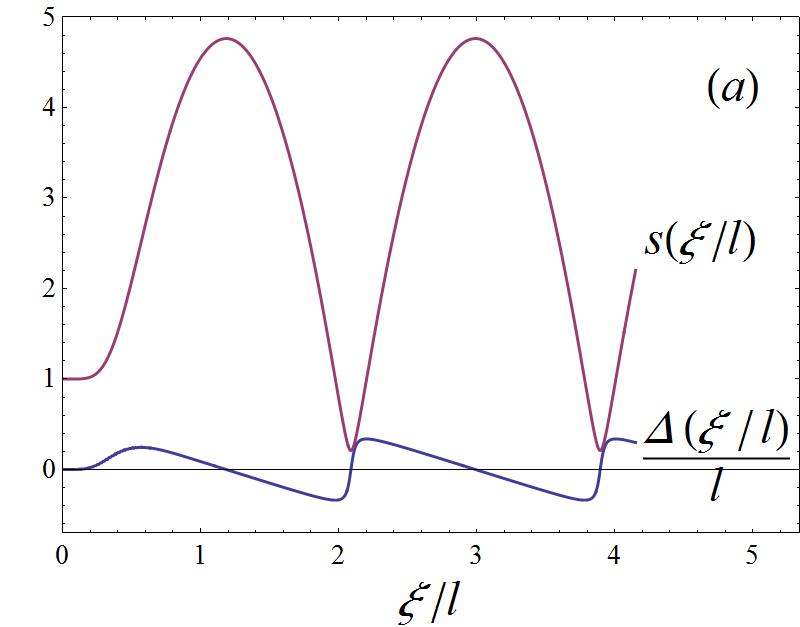
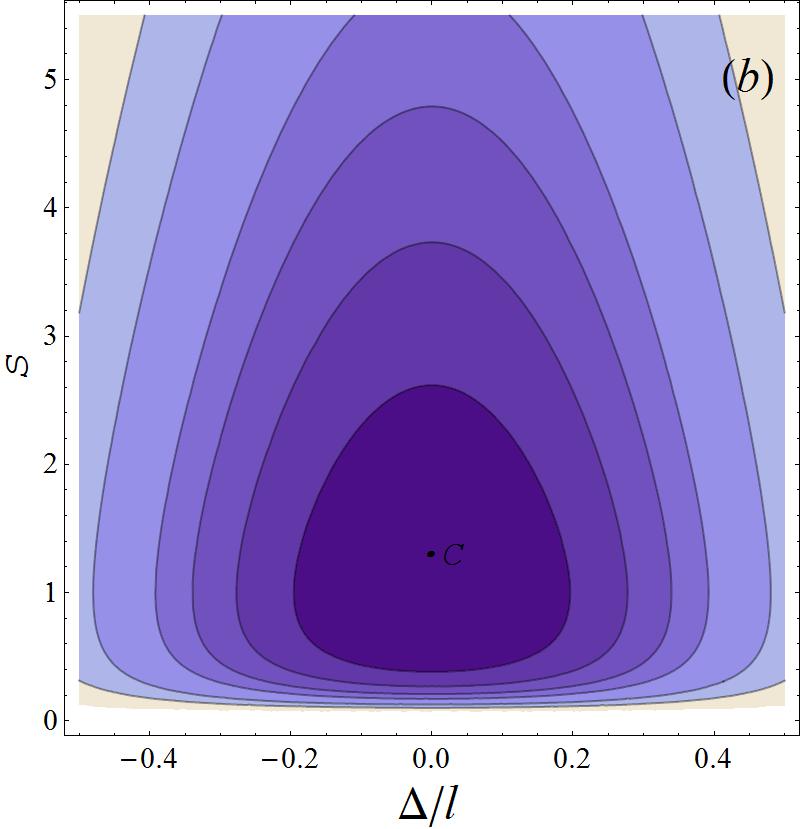
Figure 3: (a) Solution of (36) for $Ml^{2}\!=\!26$ and the $v(\xi)$ as in section IV of average intensity $I\!=\!10^{19}$W/cm². (b) Paths $P(\xi;Z)$ around the center $C$ for $Ml^{2}\!=\!26$, $v_{c}\!=\!0$.

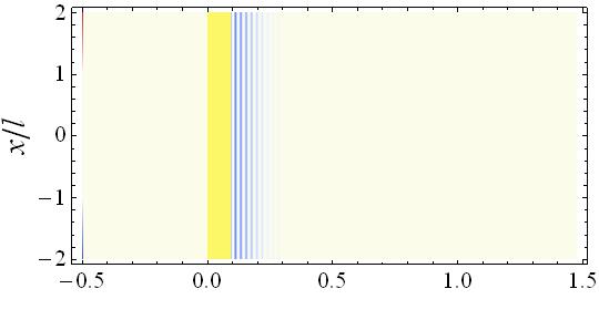
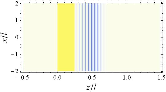
Figure 4: Normalized charge density plot $1\!-\!n_{e}/n_{0}$ under the same conditions as in fig. 7 after about 25 fs (up) and 70 fs (down), i.e. resp. before and after the maximal penetration time $\bar{t}(0)\!=\!51$fs; in the latter picture the electrons travelling backwards make light yellow-blue striped the region between the yellow and the white-blue striped ones.

III 3-dimensional effects

We now discuss the effects of the finiteness of $R$. For brevity, for any nonnegative $r,L$ we shall denote as $C_{r}$ the infinite cylinder of equation $\rho\!\leq\!r$, as $C_{r}^{\scriptscriptstyle L}$ the cylinder of equations $\rho\!\leq\!r$, $0\!\leq\!z\!\leq\!L$. The ponderomotive force of the pulse will boost forward (as in fig. 8) only the small-$Z$ electrons located within (or nearby) $C\!_{{\scriptscriptstyle R}}$. These Forward Boosted Electrons (FBE) will be thus completely expelled out of a cylinder which will reach its maximal extension $C\!_{{\scriptscriptstyle R}}^{\>\zeta}$ around the time $\bar{t}(0)$ of maximal longitudinal penetration $\zeta\!\equiv\!\hat{\Delta}[\bar{\xi}(0),\!0]$ of the $Z\!=\!0$ electrons. The displaced charges modify ${\bm{E}}$. By causality (see appendix A), for ${\bm{x}}$ near the $\vec{z}$ axis ${\bm{E}}(t,{\bm{x}})$ is the same as in the plane wave case for $t\!\lesssim\!\bar{t}(0)\!+\!R/c$, and smaller afterwards. We choose $\widetilde{n_{0}},R$ so that they fulfill

$$\frac{[t_{ex}\!-\!\bar{t}]c}{R}\sim 1,\quad r\equiv R-\frac{\zeta(t_{ex}\!-\!l/c)}{2(t_{ex}\!-\!\bar{t})}\>\theta(ct_{ex}-l)>0$$ (38)

and condition (35) for all $x\!=\!(t,{\bm{x}})$ such that $t\!\lesssim\!\bar{t}(0)\!+\!R/c$; here $\bar{t}\!\equiv\!\bar{t}(0)$, $t_{ex}\!\equiv\!t_{ex}(0)$ are the times of maximal penetration and of expulsion from the bulk of the $Z\!=\!0$ electrons [see (32)]. [As $\widetilde{n_{0}}$ grows from zero the right-hand side of (35) does as well, whereas $\bar{t}(0),t_{ex}(0)\!-\!\bar{t}(0)$ decrease]. In appendix A we show that conditions (38) respectively ensure that these FBE, at least within an inner cylinder $\rho\!\leq\!r\!\leq\!R$: i) move approximately as in section II until their expulsion; ii) are expelled before Lateral Electrons (LE), which are initially located outside the surface of $C\!_{{\scriptscriptstyle R}}$ and are attracted towards the $\vec{z}$-axis (see fig. 1.3), obstruct their way out. For the validity of our model we must a posteriori check also that the expelled $C_{r}$ electrons remain in $C\!_{{\scriptscriptstyle R}}$,

$$\mbox{ i.e. their transverse oscillations $\Delta x_{e}$ are $\ll R$}.$$ (39)

In the plane model the expelled $Z\!>\!0$ electrons cannot escape to $z\to\!-\infty$ because are decelerated by the constant electric force $\widetilde{F_{e}^{z}}(t,Z)\!=\!4\pi e^{2}\widetilde{N}(Z)\!>\!0$, see (12). The real electric force $\widetilde{F_{e}^{{\scriptscriptstyle zr}}}\!>\!0$ acting on the $C_{r}$ electrons after expulsion is generated by charges localized in $C\!_{{\scriptscriptstyle R}}$; hence $\widetilde{F_{e}^{{\scriptscriptstyle zr}}}\!\propto\!1/z_{e}^{2}$ as $z_{e}\!\to\!-\infty$, and the escape of expelled electrons is no more excluded a priori. Moreover, since $\widetilde{F_{e}^{z}}(t,\!0)\!=\!0$, it should be also $\widetilde{F_{e}^{{\scriptscriptstyle zr}}}(t,\!0)\!=\!0$, allowing the escape of the $Z\!=\!0$ electrons; by continuity there will exist some positive $Z\!_{{\scriptscriptstyle M}}\!\leq\!Z_{b}$ such that the $C_{r}^{Z_{{\scriptscriptstyle M}}}$ electrons escape to infinity. We stick to estimate $\widetilde{F_{e}^{{\scriptscriptstyle zr}}}$ on the $\vec{z}$-axis electrons; we assume that after the pulse has overcome them, they move along the $\vec{z}$-axis. Actually this will be justified below if $\hat{u}^{{\scriptscriptstyle\perp}}(l)\!\simeq\!0$, which in turn holds if, as usual, $l\!\gg\!\lambda$ [see the comments after (43)]. In fig. 5 a) we schematically depict the charge distribution expected shortly after the expulsion. The light blue area is occupied only by the ${\bm{X}}\!\in\!C_{r}^{Z\!_{{\scriptscriptstyle M}}}$ electrons. The orange area is positively charged due to an excess of ions. For any $Z$-electrons moving along the $\vec{z}$-axis consider the surfaces $S_{0},S_{1},S_{2}$ occupied at time $t$ by the ${\bm{X}}^{\prime}\!\in\!C_{r}$ electrons respectively having $Z^{\prime}\!=\!0,Z,Z_{2}(Z)$, where $Z_{2}(Z)$ is defined by the condition $\widetilde{N}(Z_{2})\!=\!2\widetilde{N}(Z)$, which ensures that the electron charges contained between $S_{0},S_{1}$ and $S_{1},S_{2}$ are equal (in the figure $S_{0},S_{1},S_{2}$ are respectively represented by the left border of the blue area, the dashed line and the solid line).

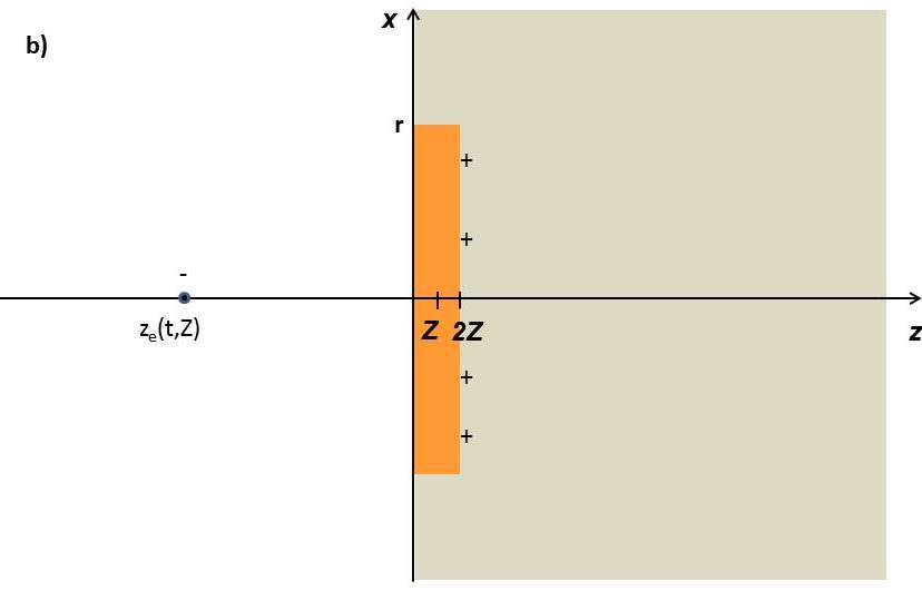
Figure 5: a) schematic picture of the expected charge distribution shortly after the expulsion (long arrows) of surface electrons; short arrows represent the inward motion of the lateral electrons; b) simplified charge distribution generating the effective potential energy.

The longitudinal electric force $\widetilde{F_{e}^{{\scriptscriptstyle zr}}}$ acting at time $t$ on this $Z$-electron is nonnegative and can be decomposed and bound as follows FioFedDeA14 :

$$0\leq\widetilde{F_{e}^{{\scriptscriptstyle zr}}}\!(t,\!Z)=-e\widetilde{E_{{\scriptscriptstyle-}}^{{\scriptscriptstyle z}}}\!(t,\!Z)\!-\!e\widetilde{E_{{\scriptscriptstyle+}}^{{\scriptscriptstyle z}}}\!(t,\!Z)\leq F_{er}^{z}\![\widetilde{\Delta}(t,\!Z),\!Z].$$

Here $\widetilde{E_{{\scriptscriptstyle-}}^{{\scriptscriptstyle z}}}(t,Z)$ stands for the part of the longitudinal electric field generated by the electrons between $S_{0},S_{2}$; since those between $S_{0},S_{1}$ have by construction the same charge as those between $S_{1},S_{2}$, but are more dispersed, it will be $-e\widetilde{E_{{\scriptscriptstyle-}}^{{\scriptscriptstyle z}}}(t,Z)\leq 0$. The part $-e\widetilde{E_{+}^{{\scriptscriptstyle z}}}(t,Z)$ of $\widetilde{F_{e}^{{\scriptscriptstyle zr}}}$ generated by the ions and the remaining electrons (at the right of $S_{2}$) will be smaller than the force $F_{er}^{z}$ generated by the charge distribution of fig. 5 b), where the remaining electrons are located farther from $(0,0,z_{e})$ (in their initial positions ${\bm{X}}^{\prime}$, not in the ones at $t$) and hence generate a smaller repulsive force. This explains the second inequality in the equation. In appendix B we show that for  $z_{e}\!\equiv\!Z\!+\!\Delta\!\leq\!0$

$$\frac{F_{er}^{z}(\Delta,\!Z)}{2\pi e^{2}}=2\widetilde{N}\!(\!Z\!)-\!\!\int_{0}^{Z_{2}(Z)}\!\!\!\!\!\!\!\!\!dZ^{\prime}\frac{\widetilde{n_{0}}(Z^{\prime})(Z^{\prime}\!-\!z_{e})}{\sqrt{\!(Z^{\prime}\!\!-\!z_{e})^{2}\!+\!r^{2}}}.\qquad$$ (40)

Commendably, $F_{er}^{z}$ is conservative, nonnegative and goes to zero as $\Delta\!\to\!-\infty$, while it reduces to zero for $Z\!=\!0$ and to $4\pi e^{2}\widetilde{N}\!(\!Z\!)$ as $r\!\to\!\infty$, as $\widetilde{F_{e}^{z}}$ in (12)₃; it becomes a function of $t$ (resp. $\xi$) through $\widetilde{\Delta}(t,Z)$ [resp. $\hat{\Delta}(\xi,\!Z)$] only. We therefore modify the dynamics outside the bulk replacing $F_{e}^{z}$ by $F_{er}^{z}$, or equivalently ${\cal U}$ by ${\cal U}\!_{r}$ in (21), where ${\cal U}\!_{r}$ is continuous and equals ${\cal U}$ for $z_{e}\!\equiv\!Z\!+\!\Delta\!\geq\!0$, and the potential energy (58) associated to $F_{er}^{z}$ for $z_{e}\!\equiv\!Z\!+\!\Delta\!\leq\!0$; there ${\cal U}\!_{r}$ is a decreasing function of $\Delta$ with finite left asymptotes (59). We will thus underestimate the final energy of the electrons, because $F_{er}^{z}$ is larger than the real electric force $\widetilde{F_{e}^{{\scriptscriptstyle zr}}}$ decelerating the electrons outside the bulk; this makes our estimates safer. In fig. 6 we plot suitably rescaled ${\cal U}$ and ${\cal U}\!_{r}$ for $\widetilde{n_{0}}(Z)=n_{0}\theta(Z)$.

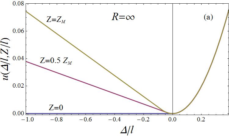
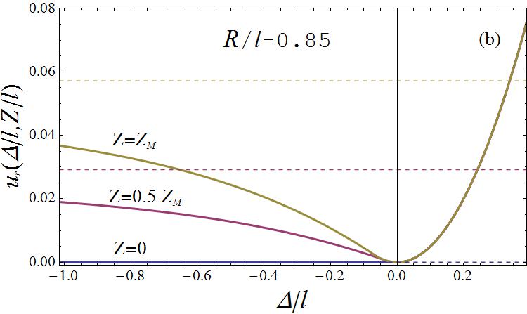
Figure 6: Rescaled longitudinal electric potential energies $u\!\equiv\!{\cal U}/4\pi n_{0}e^{2}\!l^{2}$, $u_{r}\!\equiv\!{\cal U}\!_{r}/4\pi n_{0}e^{2}\!l^{2}$ for (left) idealized plane wave $R/l\!=\!\infty$ or (right) for $R/l\!=\!0.85$, plotted as functions of $\Delta$ for $Z/Z_{{\scriptscriptstyle M}}=0,.2,.4,.6,.8,1$; the horizontal dashed lines are the left asymptotes of $u_{r}$ for the same values of $Z/Z_{{\scriptscriptstyle M}}$. Here the initial electron density is step-shaped: $\widetilde{n_{0}}(\!Z\!)\!=\!n_{0}\theta(\!Z\!)$.

After the pulse is passed we can compute $\gamma$ as a function of $\Delta,Z$ using energy conservation $m{}c^{2}\gamma\!+\!{\cal U}\!_{r}(\Delta,\!Z)\!=$const. For the expelled electrons the final relativistic factor $\gamma\!_{f}\,\!(Z)\!\equiv\!\gamma_{e}(\Delta\!=\!-\infty,\!Z)$ is the decreasing function (60). The maximum of $\gamma\!_{f}\,\!(Z)$ is $\gamma_{{\scriptscriptstyle M}}\!\equiv\!\gamma\!_{f}\,\!(0)$. Let $Z_{{\scriptscriptstyle M}}\!\leq\!Z_{b}$ be the $Z$ fulfilling $\gamma\!_{f}\,\!(Z)\!=\!1$. The estimated total number $N_{e}$, electric charge (in absolute value) $Q$, and kinetic energy ${\sf E}$ of the  ${\bm{X}}\in\!C_{r}^{Z_{{\scriptscriptstyle M}}}$  escaped electrons are thus

$$\begin{array}[]{l}N_{e}\!\sim\!\pi r^{2}\widetilde{N}\!\left(Z_{{\scriptscriptstyle M}}\!\right),\qquad Q\!\sim\!eN_{e},\\[6.0pt] {\sf E}\!\sim\!m\pi c^{2}r^{2}\!\!\!\displaystyle\int_{0}^{Z_{{\scriptscriptstyle M}}}\!\!dZ\,\widetilde{n_{0}}(Z)[\gamma\!_{f}\,\!(Z)\!-\!1].\end{array}$$ (41)

The number of escaped ${\bm{X}}^{\prime}\!\in\!C_{r}^{Z_{{\scriptscriptstyle M}}}$ electrons with $Z\!\leq\!Z^{\prime}\!\leq\!Z\!+\!dZ$ is estimated as $\pi r^{2}\widetilde{n_{0}}(Z)dZ$, that with relativistic factor between $\gamma$ and $\gamma\!+\!d\gamma$ is estimated as $dN\!=\!\pi r^{2}[\widetilde{n_{0}}(Z)/|d\gamma\!_{f}\,\!/dZ|]_{Z=\hat{Z}(\gamma)}\,d\gamma$,  where $\hat{Z}(\gamma)$ is the inverse of $\gamma\!_{f}\,(Z)$ (a strictly decreasing function, see appendix B). Hence the fraction of escaped electrons with final relativistic factor between $\gamma$ and $\gamma\!+\!d\gamma$ is estimated as $\nu(\gamma)d\gamma$, where

$$\nu(\gamma)\!\equiv\!\frac{1}{N_{e}}\frac{dN}{d\gamma}=\frac{1}{\widetilde{N}\!\!\left(Z_{{\scriptscriptstyle M}}\right)}\left.\frac{\widetilde{n_{0}}(Z)}{\left|d\gamma\!_{f}\,\!/dZ\right|}\right|_{Z=\hat{Z}(\gamma)}$$ (42)

determines the associated energy spectrum. As $\alpha^{{\scriptscriptstyle\perp}}(\xi)\!=\!\alpha^{{\scriptscriptstyle\perp}}(l)\!$ if $\xi\!\geq\!l$, by (7) the final transverse deviation of the escaped electrons will be

$$\frac{\beta_{f}^{{\scriptscriptstyle\perp}}}{\beta_{f}^{z}}(Z)\!=\!\frac{u_{f}^{{\scriptscriptstyle\perp}}}{u_{f}^{z}}(Z)\!=\!\frac{u_{f}^{{\scriptscriptstyle\perp}}}{\sqrt{\gamma_{f}^{2}(Z)\!-\!1\!-\!u_{f}^{{\scriptscriptstyle\perp}2}}},$$ (43)

where $u_{f}^{{\scriptscriptstyle\perp}}\equiv\hat{u}^{{\scriptscriptstyle\perp}}\!(l)$. This is an increasing function of $Z$, because $\gamma_{f}(Z)$ is decreasing. If  $\lambda\!\ll\!l$ then $u_{f}^{{\scriptscriptstyle\perp}}\!\simeq\!0$  (see next section), and (43) is negligible unless  $Z\!\simeq\!Z_{{\scriptscriptstyle M}}$.

III.1 Step-shaped initial density

If $\widetilde{n_{0}}(Z)\!=\!n_{0}\theta(Z)$ then $\widetilde{N}(Z)\!=\!n_{0}\theta(Z)Z$,  and for $Z\!\geq\!0$

$$\frac{F_{er}^{z}(\Delta,\!Z)}{2\pi n_{0}e^{2}}\!=\!\left\{\!\!\begin{array}[]{ll}-2\,\Delta\quad\mbox{(elastic force)},&z_{e}\!>\!0,\\[4.0pt] \!2Z\!+\!\sqrt{\!\!(\!Z\!\!+\!\!\Delta\!)^{2}\!\!+\!r^{2}}\!-\!\sqrt{\!\!(\!Z\!\!-\!\!\Delta\!)^{2}\!\!+\!r^{2}},&z_{e}\!\leq\!0.\end{array}\right.\quad$$ (46)

Since the first expression is the same as in the case $\widetilde{n_{0}}(Z)\!=\!n_{0}$, the motion of the $Z$-electron will be as in subsection II.2 until $\xi\!=\!\xi_{ex}(Z)$. The second expression goes to the constant force $4\pi n_{0}e^{2}Z$ as $r\!\to\!\infty$, as expected. The motion for $\xi\!>\!\xi_{ex}(Z)$ will be studied in detail in Fio16 ; we plot the graphs of a typical solution (until the expulsion) in fig. 7 and a few corresponding electron trajectories in Fig. 8. We can readily understand that it will be $\partial_{{\scriptscriptstyle Z}}\hat{z}_{e}(\xi,\!Z)\!\!>\!0$ for all $\xi$ and $0\!\leq\!Z\!\leq\!Z_{{\scriptscriptstyle M}}$, since this holds for $\xi\!\leq\!\xi_{ex}(Z)$ [by the comments following (36)], and both $\xi_{ex}(Z)$ and the decelerating force $F_{er}^{z}(\Delta,\!Z)$ (outside the bulk) increase with $Z$, while the speed of exit from the bulk decreases with $Z$, whence the distance between electrons with different $Z$ increases with $\xi,t$.

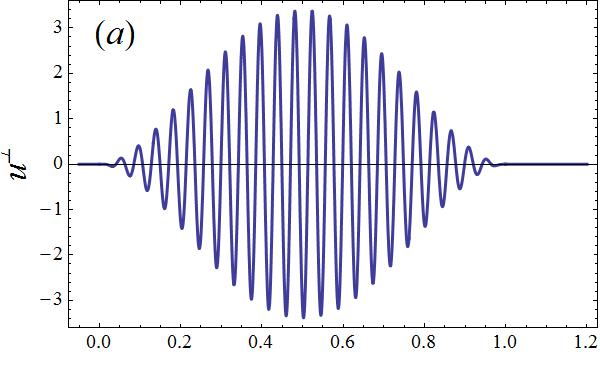
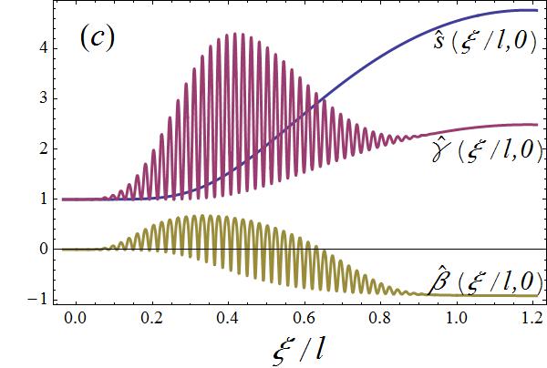
Figure 7: (a) Laser pulse of average intensity $I\!=\!10^{19}$W/cm² and shape as in section IV, with $l\!=\!18.75\mu$m. (b-c) Corresponding solution of (16-17) for initial density $\widetilde{n_{0}}(Z)\!=\!n_{0}\theta(Z)$, with $n_{0}\!=\!21\times 10^{17}$cm^-3 (i.e. $Ml^{2}\!=\!26$).

The $Z_{b}$ introduced before (23) is now the solution of the equation $\sqrt{1\!+\!v(l)}\!+\!MZ_{b}^{2}/2\!=\!h$, i.e. the $Z$ corresponding to the zero longitudinal velocity and the final value of the energy $h$ after the interaction of the pulse; one can determine $h$ evaluating $H$ at $\xi\!=\!l$, $h\!=\!\frac{1}{2}\{s(l)\!+\![1\!+\!v(l)]/s(l)\!+\!M[\Delta(l)]^{2}\}$. Hence,

$$Z_{b}=\sqrt{[\Delta(l)]^{2}+\left[s(l)\!-\!\sqrt{1\!+\!v(l)}\right]^{2}\!/2Ms(l)}.$$ (47)

$\gamma\!_{f}\,(Z)$, $\nu(\gamma)$ admit rather explicit forms (75), (78). In section IV we plot spectra $\nu(\gamma)$ corresponding to several $n_{0}$ and intensities.

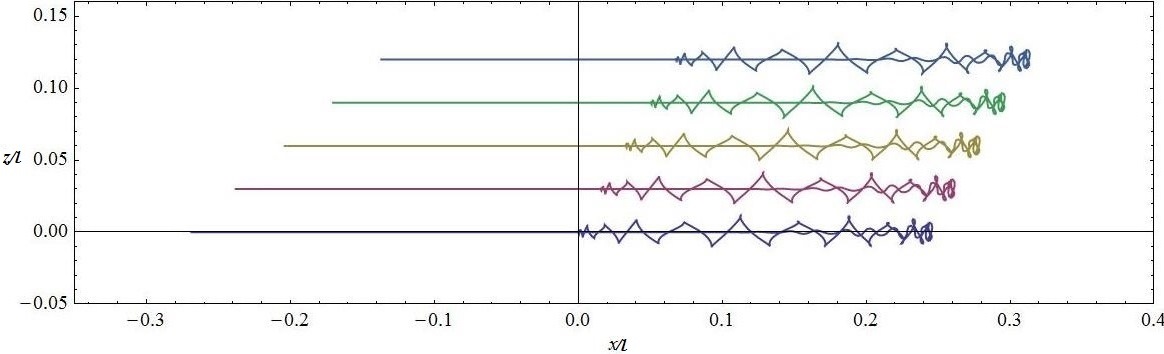
Figure 8: Trajectories gone in ca. 150 fs by electrons initially located at $Z/Z_{{\scriptscriptstyle M}}=0,0.25,0.5,0.75,1$ under conditions as in fig. 7.

Moreover,  $Q\!=\!\pi r^{2}en_{0}Z_{{\scriptscriptstyle M}}$,  ${\sf E}\!=\!\pi r^{2}n_{0}mc^{2}\!\!\int_{0}^{Z_{{\scriptscriptstyle M}}}\!\!dZ[\gamma\!_{f}\,\!(Z)\!-\!1]$. Finally, if $\xi_{ex}(0)\!<\!l$ then $\delta{\bm{u}}\!^{{\scriptscriptstyle\perp}}$ in (35) becomes

$$\delta{\bm{u}}\!^{{\scriptscriptstyle\perp}}\!(t,z)\!=\!\frac{M}{2}\!\!\displaystyle\int\limits^{ct-z}_{0}\!\!\!\!\!d\xi^{\prime}\,\frac{\hat{\bm{u}}\!^{{\scriptscriptstyle\perp}}\!(\xi^{\prime})}{s(\xi^{\prime})}\!\!\displaystyle\int\limits^{ct+z}_{0}\!\!\!\!d\xi^{\prime\prime}\,\theta\!\left[\frac{\xi^{\prime}\!\!\!+\!\xi^{\prime\prime}}{2}\!-\!\Xi(\xi^{\prime})\right]\!\!.$$ (48)

IV Numerical results

We assume for simplicity that the pulse is a slowly modulated sinusoidal function linearly polarized in the $x$ direction:  ${\bm{\epsilon}}^{{\scriptscriptstyle\perp}}(\xi)=\epsilon_{s}(\xi){\hat{\bm{x}}}\cos k\xi$,  the modulating amplitude $\epsilon_{s}(\xi)\!\geq\!0$ is nonzero only for $0\!<\!\xi\!<\!l$, and slowly varies on the scale of the period $\lambda\equiv\!2\pi/k\!\ll\!l$, i.e. $\lambda|\epsilon_{s}^{\prime}|\!\ll\!|\epsilon_{s}|$ on the support of $\epsilon_{s}$. Integrating by parts we find  ${\bm{\alpha}}^{{\scriptscriptstyle\perp}}(\xi)\!=\!{\hat{\bm{x}}}\epsilon_{s}(\xi)(\sin k\xi)/k\!+\!O(1/k^{2})$ Fio16c and, in terms of the rescaled amplitude $w(\xi)\!\equiv\!e\epsilon_{s}(\xi)/kmc^{2}$,

$$\hat{\bm{u}}^{{\scriptscriptstyle\perp}}(\xi)\!\simeq\!{\hat{\bm{x}}}\,w(\xi)\,\sin(k\xi),\qquad v(\xi)\!\simeq\!w^{2}(\xi)\,\sin^{2}(k\xi),\qquad$$ (49)

where  $a\!\simeq\!b$  means  $a\!=\!b\!+\!O(1/k^{2})$. Note that, as $\epsilon_{s}(\xi)\!=\!0$ for $\xi\!\geq\!l$, this implies $u_{f}^{{\scriptscriptstyle\perp}}\!=\!\hat{u}^{{\scriptscriptstyle\perp}}\!(l)\!\simeq\!0$,   as anticipated.

If we approximate as $\chi\!_{{\scriptscriptstyle R}}(\rho)\!\equiv\!\theta(R\!-\!\rho)$ the cutoff function in (3), the average pulse intensity on its support is  $I\!=\!c\,{\cal E}\!/\pi R^{2}l$. Here ${\cal E}$ is the EM energy carried by the pulse,

$${\cal E}=\!\int_{V}\!\!\!\!dV\frac{{\bm{E}}^{{\scriptscriptstyle\perp}2}\!\!+\!{\bm{B}}^{{\scriptscriptstyle\perp}2}}{8\pi}\!\simeq\!\frac{R^{2}}{4}\!\!\int_{0}^{l}\!\!\!\!d\xi\,{\bm{\epsilon}}^{{\scriptscriptstyle\perp}2}\!(\xi)\!\simeq\!\frac{R^{2}}{8}\!\!\int_{0}^{l}\!\!\!\!d\xi\,\epsilon_{s}^{2}\!(\xi).\qquad$$ (50)

High power lasers produce pulses where $\lambda\!\sim\!1\mu$m and $\epsilon_{s}$ is approximately gaussian, $\epsilon_{s}(\xi)\!\propto\!\exp\!\left[-(\xi\!-\!\xi_{0})^{2}/2\sigma\right]$; $\sigma$ is related to the fwhm (full width at half maximum) $l^{\prime}$ of $\epsilon_{s}^{2}$ by $\sigma\!=\!l^{\prime}{}^{2}/4\ln 2$. If initially matter is composed of atoms then $\epsilon_{s}(ct\!-\!z)$ can be considered zero where it is under the ionization threshold, because the pulse has not converted matter into a plasma yet. Hence we adopt as a modulating amplitude $\epsilon_{s}(\xi)$ the cut-off Gaussian

$$\epsilon_{g}(\xi)\!=\!b_{g}\exp\!\left[\frac{-(\xi\!-\!l/2)^{2}}{2\sigma}\right]\theta(\xi)\theta(l\!-\!\xi),\quad\sigma\!=\!\frac{l^{\prime}{}^{2}}{4\ln 2},\qquad$$ (51)

$$b_{g}^{2}\!=\!\frac{16\sqrt{\ln 2}}{\sqrt{\pi}}\frac{{\cal E}}{R^{2}l^{\prime}},\quad l^{2}=\frac{l^{\prime}{}^{2}}{\sqrt{\ln 2}}\ln\!\left[\frac{\sqrt{\ln 2}\,mc^{2}\,{\cal E}\,(e\lambda)^{2}}{U_{i}\,\sqrt{\pi}\,l^{\prime}\,(\pi Rm{}c^{2})^{2}}\right]\!,$$

where $U_{i}$ is the first ionization potential (for Helium $U_{i}\simeq 24eV$); the formula for $b_{g}^{2}$ follows replacing the Ansatz (51)₁ in (50) [neglecting the tails left out by the cutoff  $\theta(\xi)\theta(l\!-\!\xi)$]. Numerical computations are easier if we adopt Fio14JPA as $\epsilon_{s}(\xi)$ the following cut-off polynomial:

$$\epsilon_{p}(\xi)\!\equiv\!\frac{b_{p}}{4}\!\left[\!1\!-\!\left(2\xi/l_{p}\!-\!1\!\right)^{2}\!\right]^{2}\!\!\theta(\xi)\theta(l_{p}\!-\!\xi),$$ (52)

$b_{p},l_{p}$ are determined by the requirement to lead to the same fwhm and ${\cal E}$:  $b_{p}^{2}\!=\!5040\,{\cal E}/R^{2}l_{p}$ and $l_{p}\!=\!5l^{\prime}/2$.

We now present the results of extensive numerical simulations based on the experimental parameters available already now at the FLAME facility GizEtAl13 or in the near future at the ILIL facility footnote4 :  $l^{\prime}\!\simeq\!7.5\mu$m (implying $l_{p}\!=\!18.75\mu$m),  $\lambda\!\simeq\!0.8\mu$m (implying $kl_{p}\!=\!2\pi l_{p}/\lambda\!\simeq\!147$),   ${\cal E}\!=\!5$J,    and $R$ tunable by focalization in the range  $10^{-4}\div 1$ cm. We model the electron density: first as the step-shaped one   $\widetilde{n_{0}}(Z)\!=\!n_{0}\theta(Z)$ (this allows analytical derivation of more results);  then as a function smoothly increasing from zero to the asymptotic value $n_{0}$, with substantial variation in the interval  $0\!\leq\!Z\!\leq\!L\!\equiv\!20\mu$m  (as motivated by experiments, see section V), more precisely  $\widetilde{n_{0}}(Z)\!=\!n_{0}\,\theta(Z)\tanh(Z/L)$. We have numerically solved the corresponding systems (16-17) and proceeded as in section III, for $R\!=\!16,15,8,4,2,1\mu$m [resp. leading to average intensities $I/10^{19}$(W/cm${}^{2})\!\simeq\!1,1.1,4,16,64,255$], $n_{0}$ in the range $10^{17}$cm${}^{-3}\!\leq\!n_{0}\!\leq\!3\times 10^{20}$cm^-3 and $Z\!\leq\!Z_{{\scriptscriptstyle M}}$; all results follow from these solutions.

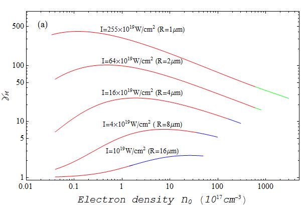
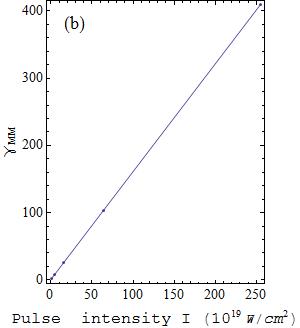
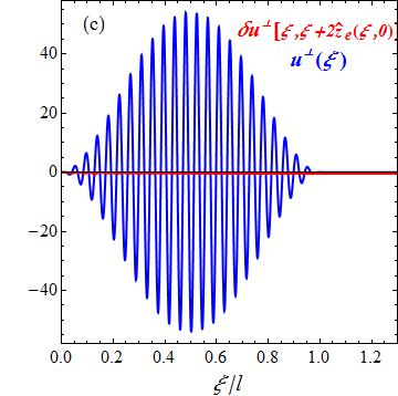
Figure 9: Left: relativistic factor $\gamma_{{\scriptscriptstyle M}}$ of the $Z\!=\!0$ expelled electrons (the maximal one) as a function of the step-shaped initial electron density $n_{0}$, for few values of the intensity $I$; the maximum of each graph is denoted as $\gamma_{{\scriptscriptstyle MM}}$. Center: $\gamma_{{\scriptscriptstyle MM}}$ vs. $I$. Right: ${\bm{u}}\!^{{\scriptscriptstyle\perp}}$ & its correction $\delta{\bm{u}}\!^{{\scriptscriptstyle\perp}}$ along the ${\bm{X}}\!\!=\!0$ electrons’ worldlines for $n_{0}\!=\!24\!\times\!10^{19}$cm^-3, $I\!=\!255\!\times\!10^{19}$W/cm²: $\delta{\bm{u}}\!^{{\scriptscriptstyle\perp}}$ is negligible.

In fig. 9-left we plot the maximal final relativistic factor $\gamma_{{\scriptscriptstyle M}}$ of the expelled electrons as a function of $n_{0}$, with the above values of $I$ and $\widetilde{n_{0}}(Z)\!=\!n_{0}\theta(Z)$; each graph stops where $n_{0}$ becomes too large for conditions (35), (38)₁, or (39) to be fulfilled and is red where condition (38)₂ is no more fulfilled. The latter prevents collisions with the LE and becomes superfluous if the target is a solid cylinder of radius $R$ (since then there are no LE) footnote5 ; the $I\!=\!64,255\!\times\!10^{19}$W/cm² graphs are plot green for densities corresponding to the lightest solids (aerogels) available today. As expected FioFedDeA14 : 1) as $n_{0}\!\to\!0$  $\gamma_{{\scriptscriptstyle M}}\!-\!1\!\propto\!n_{0}I^{2}$; 2) each graph $\gamma_{{\scriptscriptstyle M}}(n_{0};I)$ has a unique maximum $\gamma_{{\scriptscriptstyle MM}}(I)\!\equiv\!\gamma_{{\scriptscriptstyle M}}(n_{0{\scriptscriptstyle M}};I)$ at $n_{0{\scriptscriptstyle M}}\!\sim\!\bar{n}_{0}$, where $\bar{n}_{0}$ is the density making $\bar{\xi}(0)\!=\!l/2$, namely such that the $Z\!=\!0$ electrons reach the maximal penetration   $\zeta\!=\!\hat{\Delta}(l/2,0)$ when they are reached by the pulse maximum. The dependence of $\gamma_{{\scriptscriptstyle M}}$ on $n_{0}$ is anyway rather slow. The striking $\gamma_{{\scriptscriptstyle MM}}(I)\propto I$ behaviour shown in fig. 9 up-center hints at scaling laws and will be discussed elsewhere. In figures 10 we plot sample spectra $\nu(\gamma)$ for $I/10^{19}$(W/cm${}^{2})\!\simeq\!1,4,16,64$ and $\widetilde{n_{0}}$ compatible with (35), (38), (39). In table 1 we report our main predictions for the same $I$ (equivalently, $R$) and $\widetilde{n_{0}}$. The final energies of the expelled electrons range from few to about 15 MeV. The spectra (energy distributions) are rather flat for the step-shaped densities, albeit they become more peaked near $\gamma_{{\scriptscriptstyle M}}$ as $n_{0}$ grows; if $\widetilde{n_{0}}(Z)$ grows smoothly from zero to about the asymptotic value $n_{0}$ in the interval $0\!\leq\!Z\!\leq\!L\!\sim\!20\mu$m, they can be made much better (almost monochromatic) by tuning $L$. The collimation of the expelled electron bunch is very good, by (43); in all cases considered in table 1 we find deviations $\beta_{f}^{{\scriptscriptstyle\perp}}/\beta_{f}^{z}$ of $1\div 2$ milliradiants for the $(\rho,Z)\!=\!(0,0)$ and $4\div 10$ milliradiants for the $(\rho,Z)\!=\!(0,0.9Z_{{\scriptscriptstyle M}})$ expelled electrons.

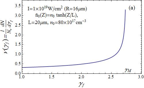
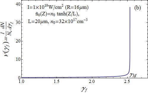
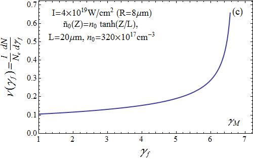
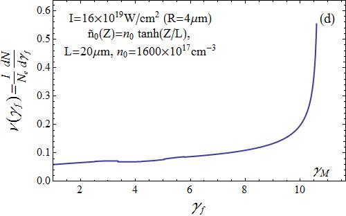
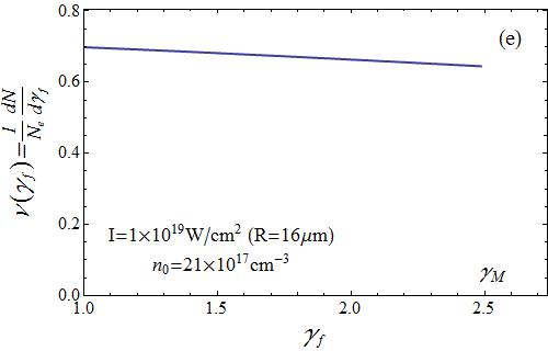
Figure 10: Sample spectra of the expelled electrons for pulse amplitudes of the form (52) with continuous initial electron densities  $\widetilde{n_{0}}(Z)\!\equiv\!n_{0}\theta(Z)\tanh(Z/L)$,  $L\!=\!20\mu$m (graphs a-d), or step-shaped initial electron densities  $\widetilde{n_{0}}\!\equiv\!n_{0}\theta(Z)$ (graphs e-f). The values of $n_{0}$ and of the average pulse intensity $I$ are the same as in Table 1.

pulse energy ${\cal E}\!\simeq\!5$J, wavelength $\lambda\!\simeq\!0.8\mu$m, fwhm $l^{\prime}\!\simeq\!7.5\mu$m, spot radius $R\!\simeq\!1\div 16\mu$m p PoP14 p PoP14 p g cp cg cp cg cp cg cp cg pulse spot radius $R\,(\mu$m) 15 15 16 16 2 2 16 16 16 16 8 8 4 4 mean intensity $I\,$(10¹⁹W/cm²) 1.1 1.1 1 1 64 64 1 1 1 1 4 4 16 16 initial el. density $n_{0}(10^{18}$cm^-3) .64 .64 .64 .64 64 64 3.2 3.2 8 8 32 32 160 160 ratio  $[t_{ex}(0)\!-\!\bar{t}({\bf 0})]c/R\!\!$ 0.8 .75 1.3 1.9 0.8 0.8 0.6 0.7 1.1 1.1 1.7 2.1 ratio  $r/R\!\!$ 0.6 0.7 1 1 0.6 0.7 0.8 0.9 0.8 1 1 1 ratio  $\Delta x_{e}^{{\scriptscriptstyle M}}/R$ .02 .02 .14 .09 .02 .19 .02 .17 .05 .04 .1 .06 maximal relativistic factor $\gamma_{{\scriptscriptstyle M}}$ 2.5 1.83 2.3 1.65 16 14 2.5 2.4 2.7 2.6 6.6 5.6 11 8.1 max. expulsion energy $H$(MeV) 1.3 0.94 1.2 0.9 8.1 7.2 1.3 1.2 1.4 1.3 3.4 2.9 5.4 4.2 tot expelled charge $|Q|(10^{-10}$C) 1.7 3.8 2.2 3.2 3.7 3.1 1.9 2.2 3.7 2.9 3.5 4 3.8 3.5 tot. exp. kin. energy ${\sf E}(10^{-4}$J) 0.7 0.7 16 12 0.8 0.8 1.6 1.1 4.5 4.0 8.6 5.8

Table 1: Sample inputs and outputs for possible experiments. In the ‘p,g’ columns the initial electron densities are step-shaped, $\widetilde{n_{0}}(Z)\!=\!n_{0}\,\theta(Z)$, and the amplitudes are resp. of the gaussian, polynomial forms (51), (52); in the ‘PoP14’ columns we report results computed in FioFedDeA14 with poorer approximation. In the ‘cg,cp’ columns the initial electron densities are the continuous ones $\widetilde{n_{0}}(Z)\!=\!n_{0}\,\theta(Z)\tanh(Z/L)$ with $L\!=\!20\mu$m, and the amplitudes are resp. of the forms (51), (52).

We now discuss the conditions guaranteeing the validity of our model. The comments after (46) show for all $\xi$ the invertibility of the maps $\hat{z}_{e}(\xi,\cdot):Z\!\mapsto\!z$ in the interval $0\!\leq\!Z\!\leq\!Z_{{\scriptscriptstyle M}}$, and therefore the self-consistency of this 2-fluid MHD model, in the step-shaped density case; numerical study of the map $\hat{z}_{e}(\cdot,\xi):Z\!\mapsto\!z$ shows that this holds true also in the continuous density case. Numerical computations show that (35) is fulfilled at least on the $Z\!\leq\!Z_{{\scriptscriptstyle M}}$ electrons’ worldlines, even with the highest densities considered here (see e.g. fig. 9 right). Finally, the data in table 1 show that (38), (39) are fulfilled.

If we choose $\epsilon_{s}(\xi)$ as the cut-off gaussian, instead of the cut-off polynomial, convergence of numerical computations is slower, but the outcomes do not differ significantly. Sample computations show that choices of other continuous $\widetilde{n_{0}}(Z)$ lead to similar results, provided the function $\widetilde{n_{0}}(Z)$ is increasing and significantly approaches the asymptotic value $n_{0}$ in the interval $0\!\leq\!Z\!\leq\!L\!\sim\!20\mu$m.

V Discussion, final remarks, conclusions

These results show that indeed the slingshot effect is a promising acceleration mechanism of electrons, in that it extracts from the targets highly collimated bunches of electrons with spectra which can be made peaked around the maximum energies by adjusting $R,\widetilde{n_{0}}$; with laser pulses of a few joules and duration of few tens of femtoseconds (as available today in many laboratories) we find that the latter range up to about ten MeV (it would increase with more energetic pulses). The spectra (distributions of electrons as functions of the final relativistic factor $\gamma_{f}$), their dependence on the electron density and pulse intensity, the collimation and the backward direction of expulsion in principle allow to discriminate the slingshot effect from the LWFA or other acceleration mechanisms. In table 1 and fig. 10 we have reported detailed quantitative predictions of the main features of the effect for some possible choices of parameters in experiments at the present FLAME, the future upgraded ILIL facilities, or similar laboratories. Low density gases or aerogels (the lightest solids available today) are targets with appropriate electron densities.

The steepest $z$-oriented density gradient of a gas sample isolated in vacuum is attained just outside a nozzle expelling a supersonic gas jet in the $xy$ plane; across the lateral border of the jet the density may vary from about zero to almost the asymptotic value $n_{0}$ in about $L\!\sim\!20\mu$m GizEtAl13 . Hence if we choose a supersonic helium jet as the laser pulse target the initial electron density is reasonably approximated by the choice $\widetilde{n_{0}}(Z)\!=\!n_{0}\,\theta(Z)\tanh(Z/L)$, and the predictions of table 1, fig. 10 (a-d) are reliable. By the way, the values of $n_{0}$ considered in table 1 are considerably higher than in typical LWFA experiments.

Step-shaped $\widetilde{n_{0}}(Z)$ are unrealistic approximations of densities of gas samples, but reasonable ones of solids (for which $\Delta Z\!\ll\!\lambda$), provided $n_{0}$ exceeds $48\!\times\!10^{18}$cm^-3, which is the electron density of aerographene (the lightest aerogel so far: mass density=0.00016 g/cm³). Silica areogels, with a wide range of densities from 0.7 to 0.001g/cm³, electron densities of the order of 10²⁰/cm^-3 and porosity from 50 nm down to 2 nm in diameter (i.e. much smaller than $\lambda$) have been produced and extensively studied PiePaj02 ; AmbBag06 . Therefore the results of the last two ‘p,g’ columns of table 1 [and the corresponding spectra, figure 10 (e)] are applicable to aerogels, while those of the first four are presently only of academic interest.

The quantitative predictions of our model are based on a rather rigorous plane-wave, 2-fluid magnetohydrodynamic model footnote6 and simple, but heuristic approximations for the 3D corrections, which certainly affect their liability. We welcome numerical 3D simulations (particle-in-cell ones, etc.) to improve the latter. Experimental tests are easily feasible with the equipments presently available in many laboratories. We welcome experiments testing the effect.

Acknowledgments. We are pleased to thank R. Fedele, L. Gizzi for stimulating discussions. G. F. acknowledges partial support by UniNA & Compagnia di San Paolo under the grant STAR Program 2013, and by COST Action MP1405 Quantum Structure of Spacetime.

Appendix A Finite $R$ conditions

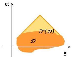
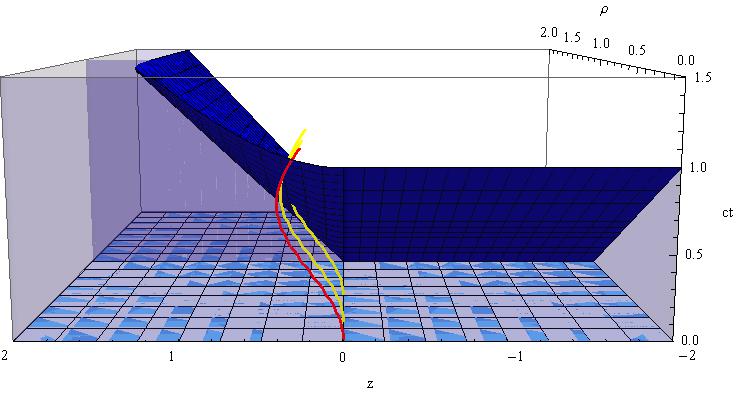
Figure 11: Left: future Cauchy development $D^{+}({\cal D})$ of a generic domain ${\cal D}$. Right: ${\cal D}^{0}_{{\scriptscriptstyle 1}}$ (light blue) and $D^{+}({\cal D}^{0}_{{\scriptscriptstyle 1}})$ (shaded region between the blue and light blue hypersurfaces) in $(\rho,z,ct)$ coordinates (we have dropped the inessential angle $\varphi$); worldlines of the ${\bm{X}}\!=\!0$ electrons (red) and of a couple of off-$\vec{z}$-axis electrons (yellow); the former remain in $D^{+}({\cal D}^{0}_{{\scriptscriptstyle 1}})$ longer.

As known, for any spacetime region ${\cal D}$ its future Cauchy development $D^{+}({\cal D})$ is defined as the set of all points $x$ for which every past-directed causal (i.e. non-spacelike) line through $x$ intersects ${\cal D}$ (see fig. 11 left). Causality implies: If two solutions of the system of dynamic equations coincide in some open spacetime region ${\cal D}$, then they coincide also in $D^{+}({\cal D})$. Therefore, knowledge of one solution determines also the other (which we will distinguish by adding a prime to all fields) in $D^{+}({\cal D})$.

In the problem at hand the solutions are exactly known for $t\!\leq\!0$, i.e. before the laser-plasma interaction begins. We use causality adopting: 1. as ${\cal D}$ a region ${\cal D}^{0}_{{\scriptscriptstyle R}}$ (see fig. 11 right) of equations $-\epsilon\!\leq\!t\!\leq\!0$ and either $\rho\!<\!R$ or $z\!>\!0$, with some $\epsilon\!>\!0$ (we can take also $\epsilon\!=\!0$ if we assign on ${\cal D}^{0}_{{\scriptscriptstyle R}}$ also the time derivatives of the $A^{\mu},{\bm{u}}$); 2. as the known solution the plane one induced (section II) by the plane transverse electromagnetic potential, which can be approximated as ${\bm{A}}\!^{{\scriptscriptstyle\perp}}(t\!,z)\!=\!{\bm{\alpha}}\!^{{\scriptscriptstyle\perp}}(ct\!-\!z)$ under the assumption (35); 3. as the unknown solution the “real” one induced by the “real” laser pulse $A^{\mu}_{f}(t,\!{\bm{x}})$, which we approximate as a potential leading to (3). It is easy to show that $D^{+}({\cal D}^{0}_{{\scriptscriptstyle R}})$ is the union of three regions, resp. of equations: a. $z\!\geq\!ct\!\geq\!0$; b. $ct\!\geq\!z\!\geq\!0$ and $\rho\!+\!\sqrt{c^{2}t^{2}\!-\!z^{2}}\!\leq\!R$; c. $t\!\geq\!0$, $z\!<\!0$ and $\rho\!+\!ct\!\leq\!R$ (see fig. 11). In $D^{+}({\cal D}^{0}_{{\scriptscriptstyle R}})$ the two solutions coincide, in particular a “real” electron worldline ${\bm{x}}_{e}^{\prime}(t,{\bm{X}})$ remains equal to the plane solution worldline ${\bm{x}}_{e}(t,{\bm{X}})$ as long as ${\bm{x}}_{e}(t,{\bm{X}})\!\in\!D^{+}({\cal D}^{0}_{{\scriptscriptstyle R}})$.

By continuity, we expect that the two solutions remain close to each other also in a neighbourhood of $D^{+}({\cal D}^{0}_{{\scriptscriptstyle R}})$. This is confirmed by estimates FioFedDeA14 involving the retarded electromagnetic potential (in the Lorentz gauge $\partial\cdot A\!=\!0$)

$$A^{\mu}\!(t,\!{\bm{x}})\!=\!A^{\mu}_{f}(t,\!{\bm{x}})\!+\!\!\int\!\!\!d^{3}x^{\prime}\frac{j^{\mu}[t_{r}(t,\!{\bm{x}}\!-\!{\bm{x}}^{\prime}),{\bm{x}}^{\prime}]}{|{\bm{x}}\!-\!{\bm{x}}^{\prime}|},\qquad$$ (53)

i.e. the general solution of the Maxwell equation $\Box A^{\mu}\!=\!4\pi j^{\mu}$ with a current $j^{\mu}(t,{\bm{x}})$ vanishing for $t\!<\!0$; here $t_{r}(t,\!{\bm{x}}\!-\!{\bm{x}}^{\prime})\!\equiv\!t\!-\!|{\bm{x}}\!-\!{\bm{x}}^{\prime}|/c$, $A^{\mu}_{f}(t,\!{\bm{x}})$ fulfills $\Box A^{\mu}_{f}\!=\!0$ (determining the $t\!\to\!-\infty$ behaviour), and ${\bm{E}}\!=\!\frac{-1}{c}\partial_{t}{\bm{A}}\!-\!\!\nabla\!\!A^{0}\!$, ${\bm{B}}\!=\!\nabla\!\times\!{\bm{A}}\!$. Since the formation of $C\!_{{\scriptscriptstyle R}}^{\>\zeta}$ is completed at $t\!=\!\bar{t}(0)$, and the ‘information’ [encoded in (53)] about the finite radius of $C\!_{{\scriptscriptstyle R}}^{\>\zeta}$ takes a time $R/c$ to go from the lateral surface $\rho\!=\!R$ to the $\vec{z}$-axis, then if eq. (38)₁ is fulfilled the ${\bm{X}}\!=\!0$ electrons (red worldline in fig. 11) move approximately as in section II until the expulsion. Similarly, the $Z\!\simeq\!0$, $\rho\!\lesssim\!r$ electrons (yellow worldlines in fig. 11) move approximately as in section II until $\bar{t}+(R\!-\!r)/c$, i.e get the main backward boost (acceleration is maximal around $\bar{t}$). Eq. (38)₂ is equivalent to

$$\begin{array}[]{llll}&t_{ex}\lesssim l/c;&\Rightarrow&r\simeq R;\\[4.0pt] \mbox{or }&0\!<\!(t_{ex}\!-\!l/c)v^{\rho}_{a}\!<\!R&\Rightarrow&r\simeq R-(t_{ex}\!-\!l/c)v^{\rho}_{a}>0.\end{array}$$ (56)

If the left-hand side of the first line is fulfilled the surface electrons are expelled while the laser pulse is still entering the bulk and thus producing an outward force that keeps the LE out of $C\!_{{\scriptscriptstyle R}}^{\>\zeta}$. Otherwise, the left-hand side of the second line ensures that the distance inward travelled by the most dangerous LE (the $Z\!=\!0$ ones) after the pulse has completely entered the bulk is less than $R$; $v^{\rho}_{a}$ stands for the average $\rho$-component of the velocity of these LE. By geometric reasons $v^{\rho}_{a}\!<\!v^{z}_{a}\!\equiv$ average $z$-component of the ${\bm{X}}\!=\!0$ electrons velocity in their backward trip within the bulk; our rough estimate $v^{\rho}_{a}\!\simeq\!v^{z}_{a}/2\!=\!\zeta/(t_{ex}\!-\bar{t})2$ gives (38)₂. Eq. (38) is thus explained.

Appendix B Finite $R$ energies

Using cylindrical coordinates $(y,\rho,\varphi)$ for ${\bm{X}}^{\prime}$, one easily finds that for $z_{e}\!\equiv\!Z\!+\!\Delta\!\leq\!0$ the electric force generated by the static charge distribution of fig. 5 b), the associated potential energy $mc^{2}{\cal U}\!_{r}$ and the left asymptotes of ${\cal U}\!_{r}$ are

$$F_{er}^{z}(\Delta,\!Z)\equiv\!\!\int_{0}^{Z_{2}(Z)}\!\!\!\!\!\!\!\!dy\,\widetilde{n_{0}}(y)\!\!\int_{0}^{r}\!\!\!d\rho\frac{2\pi e^{2}\rho(y\!-\!z_{e})}{\big{[}\rho{}^{2}\!+\!\left(y\!-\!z_{e}\right)^{2}\big{]}^{3/2}}\qquad$$

$$=\!-\!2\pi e^{2}\!\!\int_{0}^{Z_{2}(Z)}\!\!\!\!\!\!\!\!\!\!\!dy\>\frac{\widetilde{n_{0}}(y)(y\!-\!z_{e})}{\sqrt{\!(y\!-\!z_{e})^{2}\!+\!r^{2}}}+4\pi e^{2}\widetilde{N}\!(\!Z\!).\qquad\qquad$$ (57)

$${\cal U}\!_{r}(\Delta,\!Z)\equiv\displaystyle\frac{\mu}{2}\displaystyle\int_{0}^{Z_{2}(Z)}\!\!\!\!\!\!\!\!\!\!\!\!dy\,\widetilde{n_{0}}(y)\big{[}\sqrt{\!y{}^{2}\!+\!r^{2}}\qquad\qquad\qquad\qquad$$ (58)

$$\qquad\qquad\qquad\qquad\!-\!\sqrt{\!(y\!\!-\!\!Z\!\!-\!\!\Delta)^{2}\!+\!r^{2}}\big{]}\!-\!\mu\widetilde{N}\!(\!Z\!)\Delta\!-\!\mu\widetilde{{\cal N}}(Z),$$

$${\cal U}\!_{r}(-\infty,\!Z)\!=\!\displaystyle\frac{\mu}{2}\!\!\displaystyle\int_{0}^{Z_{2}(Z)}\!\!\!\!\!\!\!\!\!\!\!\!\!\!\!dy\,\widetilde{n_{0}}\!(\!y\!)\!\!\left[\!\!\sqrt{\!\!y{}^{2}\!\!+\!r^{2}}\!-\!y\right]\!+\!\mu\!\!\displaystyle\int_{0}^{Z}\!\!\!\!\!\!\!dy\,\widetilde{n_{0}}\!(\!y\!)y.\qquad$$ (59)

Here $\mu\!\equiv\!4\pi e^{2}\!/mc^{2}$. ${\cal U}\!_{r}$ is continuous in $(-Z,\!Z)$, since we have chosen ${\cal U}(-Z,Z)$ as the ($\Delta$-independent) ‘additive constants’. Energy conservation implies

$$\gamma\!+\!{\cal U}\!_{r}(\!\Delta,\!Z)\!=\!\hat{\gamma}[l,\!Z]\!+\!{\cal U}\!_{r}[\hat{\Delta}(l,\!Z),\!Z]\!=\!\hat{\gamma}[\xi_{ex}(\!Z\!),\!Z]\!+\!{\cal U}\!_{r}(\!-\!Z,\!Z).$$

The last equality holds only if $\hat{z}_{e}(l,\!Z)\!\geq\!0$, i.e. $l\!\leq\!\xi_{ex}(Z)$; the right-hand side is the electrons’ energy when expelled from the bulk. This leads to the final relativistic factor

$$\gamma\!_{f}\,\!(\!Z\!)\!\!=\!\hat{\gamma}(\!l\!,\!Z\!)\!-\!\mu\widetilde{N}\!(\!Z\!)\hat{z}_{e}\!(\!l\!,\!Z\!)\!+\!\displaystyle\frac{\mu}{2}\!\!\!\int_{0}^{Z_{2}(Z)}\!\!\!\!\!\!\!\!\!\!\!\!\!\!\!dy\,\widetilde{n_{0}}\!(\!y\!)\!\left[\!y\!\!-\!\!\sqrt{\![y\!\!-\!\!\hat{z}_{e}\!(\!l\!,\!Z\!)]^{2}\!\!+\!r^{2}}\!\right]\!$$

$$\!=\!\hat{\gamma}[\xi_{ex}\!(\!Z\!),\!Z]\!+\!\frac{\mu}{2}\!\!\!\int_{0}^{Z_{2}(Z)}\!\!\!\!\!\!\!\!\!\!\!\!\!\!\!\!dy\,\widetilde{n_{0}}\!(\!y\!)\!\!\left[y\!-\!\sqrt{\!y{}^{2}\!+\!r^{2}}\right]\!\!\quad\mbox{if }l\!\leq\!\xi_{ex}(\!Z\!).\qquad\>$$ (60)

Deriving this and the identity $\widetilde{N}[Z_{2}(Z)]\!=\!2\widetilde{N}(Z)$ we find  $\widetilde{n_{0}}[Z_{2}(Z)]\frac{dZ_{2}}{dZ}\!=\!2\widetilde{n_{0}}(Z)$  and that, as claimed, $\gamma\!_{f}\,\!(Z)$ is strictly decreasing, since $d\gamma\!_{f}\,\!\!/dZ$ is negative-definite:

$$\frac{d\gamma\!_{f}\,}{dZ}\!=\!\!\begin{array}[]{l}\frac{\partial\hat{\gamma}(l,\!Z)}{\partial Z}\!-\!\frac{\mu}{2}\!\frac{dZ_{2}}{dZ}\widetilde{n_{0}}[Z_{2}\!(\!Z\!)]\!\left[\!\sqrt{\![Z_{2}\!(\!Z\!)\!-\!\hat{z}_{e}\!(\!l\!,\!Z\!)]^{2}\!+\!r^{2}}\!\!-\!\!Z_{2}\!(\!Z\!)\!\Big{]}\right.\end{array}$$ (62)

$$\begin{array}[]{l}\!\!-\!\mu\widetilde{n_{0}}\!(\!Z\!)\hat{z}_{e}\!(\!l\!,\!Z\!)\!-\!\mu\widetilde{N}\!(\!Z\!)\frac{\partial\hat{z}_{e}\!(\!l\!,\!Z\!)}{\partial Z}\!=\!\frac{\partial\hat{\gamma}}{\partial Z}(\!l\!,\!Z\!)\!-\!\mu\widetilde{N}\!(\!Z\!)\frac{\partial\hat{z}_{e}}{\partial Z}(\!l\!,\!Z\!)\end{array}\quad$$ (64)

$$\!\!\!-\!\mu\widetilde{n_{0}}(\!Z\!)\!\left[\!\sqrt{\![Z_{2}\!(\!Z\!)\!-\!\hat{z}_{e}\!(\!l\!,\!Z\!)]^{2}\!+\!r^{2}}\!-\!Z_{2}\!(\!Z\!)\!+\!\hat{z}_{e}\!(\!l\!,\!Z\!)\right]\!\!.\qquad\quad$$ (65)

For the step-shaped initial density, setting $\phi\!\equiv\!\hat{\Delta}(l,\!Z)\!-\!Z$,

$$\begin{array}[]{l}{\cal U}\!_{r}(\Delta,\!Z)\!\!=\!\!\frac{M}{4}\!\left[(\Delta\!-\!Z)\sqrt{\!(\Delta\!-\!Z)^{2}\!+\!r^{2}}\!-\!4Z(\Delta\!+\!Z)\right.\\[6.0pt] \!+r^{2}\sinh^{\scriptscriptstyle-1}\!\!\frac{\Delta\!-\!Z}{r}\!-\!(\Delta\!+\!Z)\sqrt{\!(\Delta\!+\!Z)^{2}\!+\!r^{2}}\!-\!r^{2}\sinh^{\scriptscriptstyle-1}\!\!\frac{\Delta\!+\!Z}{r}\\[6.0pt] \left.\quad\qquad\!+2Z^{2}\!+\!2Z\sqrt{\!4Z^{2}\!+\!r^{2}}\!+\!r^{2}\sinh^{\scriptscriptstyle-1}\!\frac{2Z}{r}\right],\end{array}$$ (69)

$${\cal U}\!_{r}(-\infty,\!Z)=\begin{array}[]{l}\frac{M\!Z}{2}\!\left[\!\sqrt{\!4Z^{2}\!+\!r^{2}}\!-\!Z\!+\!\frac{r^{2}}{2Z}\sinh^{\scriptscriptstyle-1}\!\!\frac{2Z}{R}\!\right]\!\!,\end{array}\qquad\qquad$$ (71)

$$\gamma\!_{f}\,\!(Z)\!=\!\hat{\gamma}(\!l\!,\!Z\!)\!+\!\!\!\begin{array}[]{l}\frac{M}{4}\!\left\{\!\phi\sqrt{\!\phi\!+\!r^{2}}\!-\!4Z\hat{\Delta}(\!l\!,\!Z\!)\!+r^{2}\sinh^{\scriptscriptstyle-1}\!\frac{\phi}{r}\right.\end{array}\qquad$$ (73)

$$\begin{array}[]{l}\left.\!-\![\phi\!+\!2Z]\sqrt{\![\phi\!+\!2Z]^{2}\!+\!r^{2}}\!-r^{2}\sinh^{\scriptscriptstyle-1}\!\frac{\phi\!+\!2Z}{r}\right\}\end{array}\quad\qquad$$ (75)

$$\!=\!\hat{\gamma}[\xi_{ex}\!(\!Z\!)]\!+\!\!\begin{array}[]{l}M\!\!\left[\!Z^{2}\!\!-\!\frac{Z}{2}\!\sqrt{\!\!4Z^{2}\!\!+\!r^{2}}\!-\!\frac{r^{2}}{4}\sinh^{\scriptscriptstyle-1}\!\!\frac{2Z}{r}\!\right]\end{array}\>\>\mbox{if }l\!\leq\!\xi_{ex}\!(\!Z\!).$$ (77)

If $l\!\leq\!\xi_{ex}(Z)$ then  $\partial_{{\scriptscriptstyle Z}}\hat{\gamma}\!=\!0\!=\!\partial_{{\scriptscriptstyle Z}}\hat{\Delta}$ at $\xi\!=\!\xi_{ex}(Z)$,  eq. (65) reduces to  $d\gamma\!_{f}\,\!/dZ\!=\!M[Z-\sqrt{\!4Z^{2}\!+\!r^{2}}]$, and (42) to

$$1/\nu(\gamma)=M\,Z_{{\scriptscriptstyle M}}\big{[}\sqrt{\!4Z^{2}\!+\!r^{2}}\!-\!Z\big{]}_{Z=\hat{Z}(\gamma)}.$$ (78)

References

- (1) T. Tajima, J.M. Dawson, Phys.Rev.Lett. 43, 267 (1979).
- (2) D. Strickland, G. Mourou, Opt. Commun. 56 (1985), 219.
- (3) M. D. Perry, G. Mourou, Science 264 (1994), 917; and references therein.
- (4) L.M. Gorbunov, V.I. Kirsanov, Sov. Phys. JETP 66 (1987), 290.
- (5) P. Sprangle, E. Esarey, A. Ting, G. Joyce, Appl. Phys. Lett. 53, 2146 (1988).
- (6) S.P. Mangles, C.D. Murphy, Z. Najmudin, A.G. Thomas, J.L. Collier, A.E. Dangor, E.J. Divall, P.S. Foster, J.G. Gallacher, C.J. Hooker, D.A. Jaroszynski, A.J. Langley, W.B. Mori, P.A. Norreys, F.S. Tsung, R. Viskup, B.R. Walton, K. Krushelnick, Monoenergetic beams of relativistic electrons from intense laser-plasma interactions, Nature 431 (2004), 535.
- (7) C. G. R. Geddes, Cs. Tóth, J. van Tilborg, E. Esarey, C.B. Schroeder, D. Bruhwiler, C. Nieter, J. Cary, W.P. Leemans, Nature 431 (2004), 538.
- (8) J. Faure, Y. Glinec, A. Pukhov, S. Kiselev, S. Gordienko, E. Lefebvre, J.-P. Rousseau, F. Burgy, V. Malka, Nature 431 (2004), 541.
- (9) X. Wang, R. Zgadzaj, N. Fazel, Z. Li, S.A. Yi, Xi Zhang, W. Henderson, Y.-Y. Chang, R. Korzekwa, H.-E. Tsai, C.-H. Pai, H. Quevedo, G. Dyer, E. Gaul, M. Martinez, A.C. Bernstein, T. Borger, M. Spinks, M. Donovan, V. Khudik, G. Shvets, T. Ditmire, M.C. Downer, Nat. Commun. 4 (2013), article nr.: 1988.
- (10) W.P. Leemans, A.J. Gonsalves, H.-S. Mao, K. Nakamura, C. Benedetti, C.B. Schroeder, Cs. Tóth, J. Daniels, D.E. Mittelberger, S.S. Bulanov, J.-L. Vay, C.G.R. Geddes, E. Esarey, Phys. Rev. Lett. 113 (2014), 245002.
- (11) A. Irman, M.J.H. Luttikhof, A.G. Khachatryan, F.A. van Goor, J.W.J. Verschuur, H.M.J. Bastiaens, K.-J. Boller, J. Appl. Phys. 102 (2007), 024513.
- (12) C. Joshi, Scientific American 294 (2006), 40.
- (13) G. Fiore, R. Fedele, U. de Angelis, Phys. Plasmas 21 (2014), 113105.
- (14) G. Fiore, J. Phys. A: Math. Theor. 47 (2014), 225501.
- (15) G. Fiore, S. De Nicola, Nucl. Instr. Meth. Phys. Res. A, DOI: 10.1016/j.nima.2016.02.085
- (16) G. Fiore, Ricerche Mat., DOI 10.1007/s11587-016-0270-3
- (17) J. Badziak, S. Glowacz, S. Jablonski, P. Parys, J. Wolowski, H. Hora, J. Krása, L. Láska, K. Rohlena, Production of ultrahigh ion current densities at skin-layer subrelativistic laser–plasma interaction Plasma Phys. Control. Fusion 46 (2004), B541-B555.
- (18) A. A. Sahai, F. S. Tsung, A. R. Tableman, W. B. Mori, T. C. Katsouleas, Relativistically induced transparency acceleration of light ions by an ultrashort laser pulse interacting with a heavy-ion-plasma density gradient, Phys. Rev. E 88, 043105 (2013)
- (19) A. A. Sahai, Motion of the plasma critical layer during relativistic-electron laser interaction with immobile and comoving ion plasma for ion acceleration, Physics of Plasmas 21, 056707 (2014); doi: 10.1063/1.4876616
- (20) G. Fiore, Travelling waves and a fruitful ‘time’ reparametrization in relativistic electrodynamics, in preparation.
- (21) G. Fiore, Acta Appl. Math. 132 (2014), 261.
- (22) G. Fiore A plane-wave model of the impact of short laser pulses on plasmas, in preparation.
- (23) L.A. Gizzi, C. Benedetti, C.A. Cecchetti, G. Di Pirro, A. Gamucci, G. Gatti, A. Giulietti, D. Giulietti, P. Koester, L. Labate, T. Levatoy, N. Pathak, F. Piastra, Appl. Sci., 3 (2013), 559. doi:10.3390/app3030559.
- (24) A.C. Pierre, G.M. Pajonk, Chem. Rev. 102, 4243 (2002).
- (25) A.P. Ambekar, P. Bagade, Popular Plastics & Packaging, 51, 96-102 (2006).
- (26) P. L. Bhatnagar, E. P. Gross, M. Krook,
- (27) G. Fiore , A. Maio, P. Renno, Ric. Mat. 63 (2014), Suppl. 1, 157-164; and references therein.
- (28) grows with the oscillation amplitude , but goes to the nonrelativistic period as .
- (29) If , then while the pulse is passing can be neglected, and the motion of the electron is close to the one in vacuum; the backward acceleration takes place afterwards and is due only to , hence the final energy is smaller. Whereas if - which was the standard situation in laboratories until a couple of decades ago - then oscillates many times about 0, , and the backward acceleration is washed out.
- (30) Albeit the pump (3) violates the Maxwell equations (due to the -dependence), we adopt it as for our purposes it is essentially equivalent to one that fulfills the Maxwell equations and at the time of impact coincides with it in the main part of its support, while rapidly decaying outside (this and similar schematizations, e.g. the paraxial one, are currently used in the literature).
- (31) reduce to the of Fio14JPA if .
- (32) L. Gizzi, private communication.
- (33) We thank L. Gizzi for this remark.
- (34) There is no need of a recourse to kinetic theory taking collisions into account, e.g. by BGK BhaGroKro54 equations or effective linear inheritance relations FioMaiRen14 .