Ising model in clustered scale-free networks

Abstract

The Ising model in clustered scale-free networks has been studied by Monte Carlo simulations. These networks are characterized by a degree distribution of the form $P(k)\sim k^{-\gamma}$ for large $k$. Clustering is introduced in the networks by inserting triangles, i.e., triads of connected nodes. The transition from a ferromagnetic (FM) to a paramagnetic (PM) phase has been studied as a function of the exponent $\gamma$ and the triangle density. For $\gamma>3$ our results are in line with earlier simulations, and a phase transition appears at a temperature $T_{c}(\gamma)$ in the thermodynamic limit (system size $N\to\infty$). For $\gamma\leq 3$, a FM–PM crossover appears at a size-dependent temperature $T_{\rm co}$, so that the system remains in a FM state at any finite temperature in the limit $N\to\infty$. Thus, for $\gamma=3$, $T_{\rm co}$ scales as $\ln N$, whereas for $\gamma<3$, we find $T_{\rm co}\sim JN^{z}$, where the exponent $z$ decreases for increasing $\gamma$. Adding motifs (triangles in our case) to the networks causes an increase in the transition (or crossover) temperature for exponent $\gamma>3$ (or $\leq 3$). For $\gamma>3$, this increase is due to changes in the mean values $\langle k\rangle$ and $\langle k^{2}\rangle$, i.e., the transition is controlled by the degree distribution (nearest neighbor connectivities). For $\gamma\leq 3$, however, we find that clustered and unclustered networks with the same size and distribution $P(k)$ have different crossover temperature, i.e., clustering favors FM correlations, thus increasing the temperature $T_{\rm co}$. The effect of a degree cutoff $k_{\rm cut}$ on the asymptotic behavior of $T_{\rm co}$ is discussed.

I Introduction

Many natural and artificial systems have a network structure, with nodes representing typical system units and edges playing the role of interactions between connected pairs of units. Complex networks can be used to model various kinds of real-life systems (social, economic, technological, biological), and to analyze processes taking place on them Strogatz (2001); Albert and Barabási (2002); Dorogovtsev and Mendes (2003); Newman (2010); Cohen and Havlin (2010). In recent years, various network models have been designed capturing aspects of real systems, thus allowing to explain empirical data in several fields. This is the case of small-world Watts and Strogatz (1998) and scale-free networks Barabási and Albert (1999), which provide us with the underlying topological structure to analyze processes such as signal propagation Watts and Strogatz (1998); Herrero (2002a), as well as the spread of information Pandit and Amritkar (2001); Lahtinen et al. (2001), opinions Candia (2007) and infections Moore and Newman (2000); Kuperman and Abramson (2001). These types of networks have been also used to study statistical physical problems as percolation Moore and Newman (2000); Newman and Watts (1999) and cooperative phenomena Barrat and Weigt (2000); Leone et al. (2002); Herrero (2002b); Castellano et al. (2005); Dorogovtsev et al. (2008); Herrero (2009a); Ostilli et al. (2011).

In scale-free (SF) networks the degree distribution $P(k)$, where $k$ is the number of links connected to a node, has a power-law decay $P_{\rm sf}(k)\sim k^{-\gamma}$ Dorogovtsev and Mendes (2002); Goh et al. (2002). This type of networks have been found in several real-life systems, such as the internet Siganos et al. (2003), the world-wide web Albert et al. (1999), protein interaction networks Jeong et al. (2001), and social systems Newman (2001). In both natural and artificial systems, the exponent $\gamma$ controlling the degree distribution is usually in the range $2<\gamma<3$ Dorogovtsev and Mendes (2002); Goh et al. (2002). The origin of power-law degree distributions was studied by Barabási and Albert Barabási and Albert (1999), who found that two ingredients can explain the scale-free nature of networks, namely growth and preferential attachment. More general models based on these ingredients have appeared later in the literature Krapivsky et al. (2000); Hébert-Dufresne et al. (2011). One can also deal with equilibrium SF networks, defined as statistical ensembles of random networks with a given degree distribution $P_{\rm sf}(k)$, for which one may analyze several properties as a function of the exponent $\gamma$ Dorogovtsev and Mendes (2002); Bogacz et al. (2006).

Many real-life networks include clustering, i.e., the probability of finding loops of small size is larger than in random networks. This has been in particular quantified by the so-called clustering coefficient, which measures the likelihood of “triangles” in a network Newman (2010). Most network models employed in the past did not include clustering. Some of them, such as the Watts-Strogatz small-world model Watts and Strogatz (1998) show clustering, but are not well-suited as models of most actual networks. Several computational models of clustered networks have been defined along the years Holme and Kim (2002); Klemm and Eguiluz (2002); Serrano and Boguñá (2005), but in general their properties cannot be calculated by analytical procedures. In last years, it was shown that generalized random graphs can be generated incorporating clustering in such a way that exact formulas can be derived for many of their properties. This is the case of the networks defined by Newman Newman (2009) and Miller Miller (2009).

Cooperative phenomena in complex networks are known to display characteristics related to the particular topology of these systems Dorogovtsev et al. (2008). The Ising model on SF networks has been studied by using several theoretical techniques Leone et al. (2002); Dorogovtsev et al. (2002); Iglói and Turban (2002); Herrero (2004); Dommers et al. (2010); Menche et al. (2011), and its critical behavior was found to depend on the exponent $\gamma$. Two different regimes appear for uncorrelated networks. On one side, for an exponent $\gamma>3$, the average value $\langle k^{2}\rangle$ is finite in the large-size limit, and there appears a ferromagnetic (FM) to paramagnetic (PM) transition at a finite temperature $T_{c}$. On the other side, when $\langle k^{2}\rangle$ diverges (as happens for $\gamma\leq 3$), the system remains in its ordered FM phase at any temperature, so that there is no phase transition in the thermodynamic limit. The antiferromagnetic Ising model has been also studied in scale-free networks, where spin-glass phases have been found Bartolozzi et al. (2006); Herrero (2009b).

All this refers to unclustered random networks with a power-law degree distribution. One may ask how this picture changes when the networks are clustered, i.e., the clustering coefficient has a non-negligible value. In principle, one expects that the presence of small loops in the networks will enhance correlations between spins located on network nodes, thus favoring ordered schemes such as an FM pattern. Thus, the effects of clustering on various cooperative phenomena in complex networks have been studied earlier. This is the case of percolation Gleeson (2009); Gleeson et al. (2010); Karrer and Newman (2010); Allard et al. (2012), epidemics Miller (2009); Wang et al. (2012); Molina and Stone (2012), and dynamical processes Hebert-Dufresne et al. (2010); Melnik et al. (2011). Yoon et al. Yoon et al. (2011) studied the Ising model on networks with arbitrary distribution of motifs using an analytical procedure, the so-called belief-propagation algorithm. For the networks considered in that paper, where the thermodynamic limit is well defined ($T_{c}$ converges for $N\to\infty$), these authors found that clustering increases the critical temperature in comparison with tree-like networks with the same mean degree, but does not change the critical behavior.

In this paper we study the FM-PM transition for the Ising model in scale-free networks with clustering, which is realized by introducing triangles in the networks, i.e., three-membered loops. Several values of the exponent $\gamma$ are considered, as well as various concentrations of triangles. We employ Monte Carlo (MC) simulations to obtain the transition temperature, when it is well defined (for $\gamma>3$ ), and to derive the size dependence of the crossover temperature for cases where $\langle k^{2}\rangle$ diverges as $N\to\infty$ ($\gamma\leq 3$).

The paper is organized as follows. In Sec. II we describe the clustered networks considered here. In Sec. III we present the computational method employed to carry out MC simulations. In Sec. IV we present results of the simulations and a discussion for the different parameter regions, depending on the value of the exponent $\gamma$ ($>3$, $=3$, or $<3$). The paper closes with a summary in Sec. V.

II Scale-free networks with clustering

We consider clustered networks with a degree distribution $P(k)$ that follows the power-law dependence $P_{\rm sf}(k)\sim k^{-\gamma}$ for large degree $k$. Clustering is included by inserting triangles in the networks, i.e., triads of connected nodes. Other kinds of polygons (squares, pentagons, …) can be introduced to study their effect on critical phenomena in physical systems, but we choose triangles since they cause stronger correlations between entities defined on network sites, as in the case of the Ising model considered here.

We generate networks by following the method proposed by Newman Newman (2009), where one separately specifies the number of edges and the number of triangles. This procedure allows one to generalize random graphs to incorporate clustering in a simple way, so that exact formulas can be derived for many properties of the resulting networks Newman (2009).

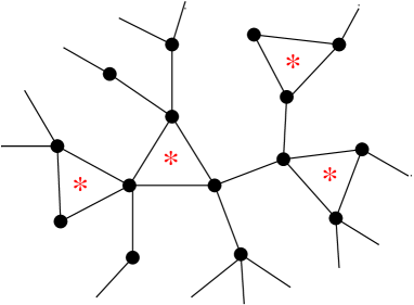
Figure 1: Schematic representation of a typical network considered in this work, for which one separately specifies the number of single links and triangles attached to each node. Triangles are indicated by asterisks (*).

For a network of size $N$ (number of nodes), we call $t_{i}$ the number of triangles in which node $i$ takes part, and $s_{i}$ the number of single edges not included in the triangles. This means that edges within the triangles are listed separately from single links. Thus, a single link can be viewed as a network element joining together two nodes and a triangle as an element connecting three nodes. The degree $k_{i}$ of node $i$ is then $k_{i}=s_{i}+2\,t_{i}$, as each triangle connects it to two other nodes. A picture of such a network is presented in Fig. 1, where triangles are indicated with asterisks (*).

To generate the networks, we first define the edges. We assign to each node $i$ a random number $s_{i}$, which represents the number of outgoing links from this node (stubs). The set of numbers $\{s_{i}\}_{i=1}^{N}$ (with $s_{i}\geq k_{0}$, the minimum allowed degree) is taken from the probability distribution $P_{\rm sf}(s)\sim s^{-\gamma}$ Newman (2005), giving a total number of stubs $K=\sum_{i=1}^{N}s_{i}$. We impose the restriction that $K$ must be an even integer. Then, we connect stubs at random (giving a total of $L=K/2$ connections), with the conditions: (i) no two nodes can have more than one bond connecting them (no multiple connections), and (ii) no node can be connected by a link to itself (no self-connections).

In a second step we introduce triangles into the networks. Their number $N_{\Delta}$ is controlled by the parameter $\nu$, which gives the mean number of triangles in which a generic node is included ($N_{\Delta}=\frac{1}{3}N\nu$). The number of triangles $t_{i}$ associated to a node $i$ is drawn from a Poisson distribution $Q(t)={\rm e}^{-\nu}\nu^{t}/t!$. Thus, we have $t_{i}$ “corners” associated to node $i$, and the total number is $T=\sum_{i=1}^{N}t_{i}=3N_{\Delta}$. We impose the condition that $T$ be a multiple of 3. Then, we take triads of corners uniformly at random to form triangles, taking into account conditions (i) and (ii) above to avoid multiple and self-connections. Note that single links can by chance form triangles. Calling $N_{t}$ the number of such triangles, their density $N_{t}/N$ for a given mean degree $\langle k\rangle$ vanishes as $N\to\infty$. In fact, $N_{t}/N$ scales as $1/N$ for large $N$ Newman (2009, 2010); Yoon et al. (2011).

In complex networks, one usually defines the clustering coefficient $C$ as the ratio $C=3N_{\Delta}/N_{3}$, where $N_{3}$ is the number of connected triplets Newman (2010):

$$N_{3}=N\sum_{k}\frac{k(k-1)}{2}\,P(k)=\frac{1}{2}N\left(\langle k^{2}\rangle-\langle k\rangle\right)\,.$$ (1)

Thus, for the networks discussed here, we have

$$C=\frac{2\nu}{\langle k^{2}\rangle-\langle k\rangle}\;,$$ (2)

and the clustering coefficient can be changed as a function of the parameter $\nu$.

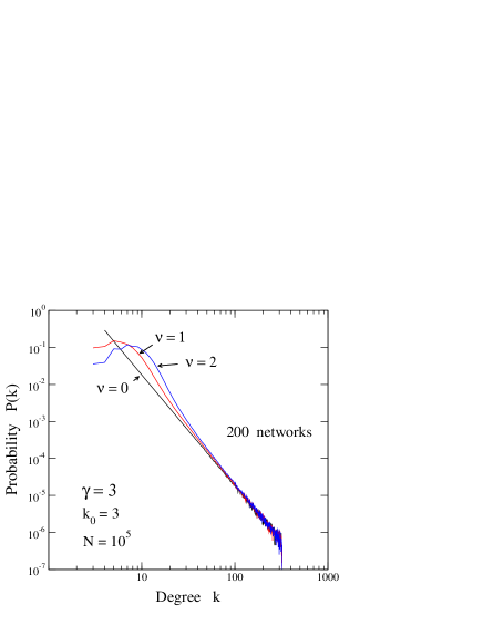
Figure 2: Probability density as a function of the degree $k$ for networks with $\gamma=3$, minimum degree $k_{0}$ = 3, and $N=10^{5}$ nodes. The data shown are an average over 200 network realizations for each value of the parameter $\nu$ = 0, 1, and 2.

Aside from $\gamma$ and the triangle density $\nu$, our networks are defined by the minimum degree $k_{0}$. Since we are interested in finite-size effects, the network size $N$ is also an important variable in our discussion. The degree distribution $P(k)$ obtained for networks generated by following the procedure described above is presented in Fig. 2. In this figure, we have plotted $P(k)$ for networks including $10^{5}$ nodes, with $\gamma=3$ and $k_{0}=3$. Each curve corresponds to a particular value of the parameter $\nu$ = 0, 1, and 2, including in each case an average over 200 network realizations. Comparing the curves corresponding to different $\nu$ values, one observes that the introduction of triangles in the networks causes clear changes in the distribution $P(k)$ for small $k$ values. However, for large degrees, the distribution is found to follow the dependence $P_{\rm sf}(k)\sim k^{-\gamma}$ typical of scale-free networks, with $\gamma=3$ in the present case. This could be expected, since the Poisson distribution $Q(t)$ associated to the triangles has a much faster exponential-like decay for large $t$. In the three cases shown in Fig. 2 there appears an effective cutoff $k_{\rm cut}\gtrsim 300$, which is related to the finite size $N$ of the networks (see below). We note that a maximum degree $k_{\rm cut}$ was explicitly introduced earlier in scale-free networks for computational convenience Herrero (2004).

An important characteristic of the considered networks, that will be employed below to discuss the results of the Ising model, is the mean degree $\langle k\rangle$. For scale-free networks with $\nu=0$, the mean degree is given by

$$\langle k\rangle_{\infty}=\sum_{k=k_{0}}^{\infty}k\,P_{\rm sf}(k)\approx k_{0}\,\frac{\gamma-1}{\gamma-2}\,,$$ (3)

where the last expression is obtained by replacing the sum by an integral, which is justified for large $N$. Note that we assume here $\gamma>2$ and that the distribution $P_{\rm sf}(k)$ is normalized to unity (for $\gamma\leq 2$ the mean degree $\langle k\rangle$ diverges in the large-size limit: $\langle k\rangle_{\infty}\to\infty$). Then, for our networks including triangles, one has

$$\langle k\rangle_{\infty}\approx 2\,\nu+k_{0}\,\frac{\gamma-1}{\gamma-2}\,.$$ (4)

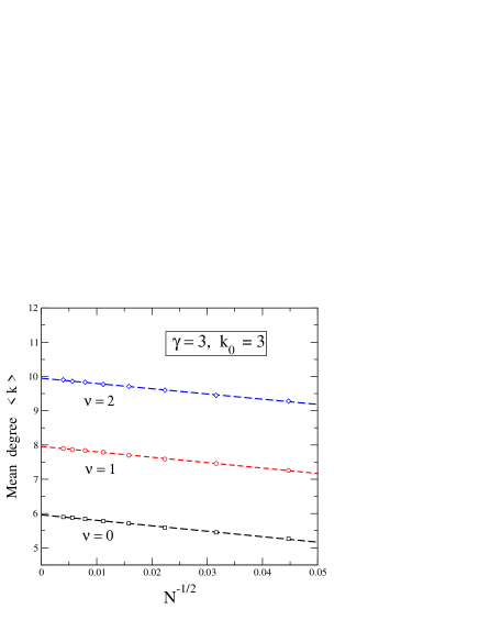
Figure 3: Mean degree $\langle k\rangle$ as a function of $N^{-1/2}$ for networks with $\gamma=3$, $k_{0}=3$, and three values of $\nu$: 0 (squares), 1 (circles), and 2 (diamonds). Error bars of the simulations results are less than the symbol size. Lines are fits to the expression $\langle k\rangle=a+b\,N^{-1/2}$.

For finite networks, a size effect is expected to appear in the mean degree, as a consequence of the effective cutoff appearing in the degree distribution (see Fig. 2). This is shown in Fig. 3, where we present $\langle k\rangle$ vs $N^{-1/2}$, for our generated networks with $\gamma=3$ and $k_{0}=3$. The mean degree decreases as $N^{-1/2}$ increases, i.e., $\langle k\rangle$ increases as the system size is raised. The data shown in Fig. 3 for $\nu$ = 0, 1, and 2, follow a linear dependence, and in fact can be fitted as $\langle k\rangle=a+b\,N^{-1/2}$, at least in the region plotted in the figure ($N>500$). The fit parameter $a$ is close to the mean degree $\langle k\rangle_{\infty}$ given in Eq. (4), and the small difference is mainly due to the replacement of sums by integrals in the derivation of that equation. Note that for $\gamma=3$, $\nu=0$ and $k_{0}=3$, Eq. (4) yields $\langle k\rangle_{\infty}$ = 6. The slope $b$ obtained from the linear fits turns out to be the same (within statistical noise) for the three cases shown in Fig. 3.

This size dependence of $\langle k\rangle$ can be understood by noting that the effective cutoff $k_{\rm cut}$ appearing in a power-law degree distribution is related with the network size $N$ by the expression Dorogovtsev et al. (2002); Iglói and Turban (2002)

$$\sum_{k_{\rm cut}}^{\infty}P_{\rm sf}(k)=\frac{c}{N}\;,$$ (5)

where $c$ is a constant on the order of unity. From this expression, one can derive for $\gamma=3$ (see the Appendix):

$$\langle k\rangle\approx\langle k\rangle_{\infty}\left[1-\left(\frac{c}{N}\right)^{\frac{1}{2}}+{\cal O}\left(\frac{1}{N}\right)\right]\;.$$ (6)

Comparing with the fit shown in Fig. 3, one finds $c\approx 7$, which introduced into Eq. (33) yields for the cutoff $k_{\rm cut}\approx 360$, in line with the results shown in Fig. 2, thus providing a consistency check for our arguments.

For scale-free networks with an exponent $\gamma<3$, Catanzaro et al. Catanzaro et al. (2005) found that appreciable correlations appear between degrees of adjacent nodes when no multiple and self-connections are allowed. Such degree correlations can be avoided by assuming a cutoff $k_{\rm cut}\sim N^{1/2}$. Thus, for $\gamma<3$ we generate here networks with cutoff $k_{\rm cut}=N^{1/2}$. For the clustered networks considered here, generated as in Ref. Newman (2009), the presence of triangles introduces degree correlations between nodes forming part of a triangle in the network.

III Simulation method

On the networks defined in Sec. II, we consider a spin model given by the Hamiltonian

$$H=-\sum_{i<j}J_{ij}S_{i}S_{j}\,,$$ (7)

where $S_{i}=\pm 1$ ($i=1,...,N$) are Ising spin variables, and the coupling matrix $J_{ij}$ is given by

$$J_{ij}\equiv\left\{\begin{array}[]{ll}J(>0),&\mbox{if $i$ and $j$ are connected,}\\ 0,&\mbox{otherwise.}\end{array}\right.$$ (8)

This model has been studied by means of Monte Carlo simulations, sampling the configuration space by using the Metropolis local update algorithm Binder and Heermann (2010). We are particularly interested in the behavior of the magnetization $M=\sum_{i=1}^{N}S_{i}/N$. For a given set of parameters ($\gamma$, $\nu$, $k_{0}$) defining the networks, the average value $\langle M\rangle$ has been studied as a function of temperature $T$ and system size $N$. This allows us to investigate the transition from a FM ($\langle M\rangle\neq 0$) to a PM ($\langle M\rangle$ = 0) regime as $T$ is increased.

Depending on the value of the exponent $\gamma$ defining the power-law distribution of single edges, two different cases are found Leone et al. (2002); Dorogovtsev et al. (2002); Herrero (2004). First, for $\gamma>3$, one expects a phase transition with a well-defined transition temperature $T_{c}$ ($<\infty$) in the thermodynamic limit $N\to\infty$. Second, for $\gamma\leq 3$ a FM–PM crossover is known to appear for scale-free networks, with a crossover temperature $T_{\rm co}(N)$ increasing with system size and diverging to infinity as $N\to\infty$.

For the cases where a FM–PM transition occurs in the thermodynamic limit ($\gamma>3$), the transition temperature $T_{c}$ has been obtained here by using Binder’s fourth-order cumulant Binder and Heermann (2010)

$$U_{N}(T)\equiv 1-\frac{\langle M^{4}\rangle_{N}}{3\langle M^{2}\rangle^{2}_{N}}\,,$$ (9)

The average values in this expression are taken over different network realizations and over different spin configurations for a given network at temperature $T$. In this case, the transition temperature is obtained from the unique crossing point of the functions $U_{N}(T)$ for several system sizes $N$ Herrero (2002b, 2004).

In the second case ($\gamma\leq 3$), the size-dependent crossover temperature $T_{\rm co}(N)$ has been obtained from the maximum of the magnetization fluctuations $(\Delta M)^{2}_{N}$ as a function of temperature, with

$$(\Delta M)^{2}_{N}=\langle M^{2}\rangle_{N}-\langle M\rangle^{2}_{N}\,.$$ (10)

We note that $T_{\rm co}$ values derived by using this criterion agree within error bars with those found from the maximum derivative of the heat capacity Herrero (2004).

The largest networks considered here included about $10^{5}$ sites. Such network sizes were employed in particular to study the dependence of $T_{\rm co}$ on $N$ for $\gamma\leq 3$. For the cases where a phase transition exists in the thermodynamic limit ($\gamma>3$), sizes around $4\times 10^{4}$ nodes were considered. The results presented below were obtained by averaging in each case over 800 networks, except for the largest system sizes, for which 400 network realizations were generated. Similar MC simulations have been carried out earlier to study ferromagnetic Herrero (2002b, 2004) and antiferromagnetic Herrero (2008, 2009b) Ising models in complex networks.

IV Results and discussion

IV.1 Case $\gamma>3$

For unclustered scale-free networks with an exponent $\gamma>3$, the average value $\langle k^{2}\rangle$ converges to a finite value as $N\to\infty$. In this case, analytical calculations Leone et al. (2002); Dorogovtsev et al. (2002) and Monte Carlo simulations Herrero (2004) predict a well-defined FM–PM transition temperature $T_{c}$ given by

$$\frac{J}{T_{c}}=\frac{1}{2}\ln\left(\frac{\langle k^{2}\rangle}{\langle k^{2}\rangle-2\langle k\rangle}\right)\;.$$ (11)

This equation is equivalent to Eq. (56) in Ref. Yoon et al., 2011.

For the clustered networks considered here with $\gamma>3$, we have calculated $T_{c}$ from the Binder’s cumulant $U_{N}$ for several values of the triangle density $\nu$ and minimum degree $k_{0}>1$. In each case, four different network sizes were considered. In all these cases, a well defined transition temperature was found from the crossing point of the curves $U_{N}(T)$ for different sizes $N$, as in Ref. Herrero, 2004. We note that $\langle k^{2}\rangle-2\langle k\rangle>0$ for $k_{0}>1$, and $T_{c}$ is well defined by Eq. (11) . For $k_{0}=1$, the simulated networks consist of many disconnected components, and Binder’s cumulant $U_{N}(T)$ does not give a unique crossing point for different system sizes $N$.

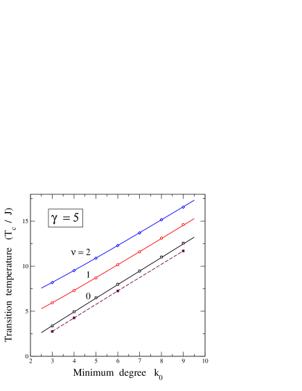
Figure 4: Transition temperature $T_{c}$ for networks with $\gamma=5$ as a function of the minimum degree $k_{0}$. Open symbols represent results of MC simulations, as obtained from Binder’s cumulant for $\nu$ = 0 (squares), 1 (circles), and 2 (diamonds). Error bars are less than the symbol size. Solid lines were derived from the analytical expression given in Eq. (11), using values of $\langle k\rangle$ and $\langle k^{2}\rangle$ obtained from Eqs. (4) and (14). Solid squares are data obtained in Ref. Herrero, 2004 for unclustered networks ($\nu$ = 0). The dashed line is a guide to the eye.

Going to the results of the present MC simulations, in Fig. 4 we present the transition temperature $T_{c}$ as a function of the minimum degree $k_{0}$ for an exponent $\gamma=5$, and three values of the triangle density $\nu$ = 0, 1, and 2. In the three cases we observe a linear increase of $T_{c}$ for rising $k_{0}$. The case $\nu=0$ corresponds to a power-law degree distribution $P_{\rm sf}(k)\sim k^{-\gamma}$ (unclustered networks). Values of $T_{c}$ found here for these networks are somewhat higher than those obtained in Ref. Herrero, 2004, by an amount $\Delta T_{c}\sim 0.6\,J$, due to the strict degree cutoff $k_{\rm cut}$ employed in that work. These earlier results are shown in Fig. 4 as open symbols. For $\nu=1$ we find $T_{c}$ values higher than for $\nu=0$, and the transition temperature increases further, by the same amount, for $\nu=2$.

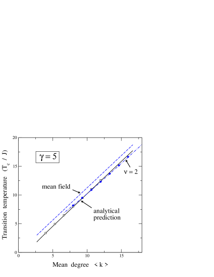
Figure 5: Transition temperature $T_{c}$ for scale-free networks with $\gamma=5$ as a function of the mean degree $\langle k\rangle$. Data points are results for networks with $\nu$ = 0 (open squares) and $\nu$ = 2 (solid diamonds). Error bars are less than the symbol size. Solid and dashed-dotted lines are analytical predictions from Eq. (11) for $\nu$ = 0 and 2, respectively. The dashed line represents the mean-field result given by Eq. (15).

Looking at Eq. (11), one expects that $T_{c}$ should have an explicit dependence on $\langle k\rangle$ and $\langle k^{2}\rangle$, rather than the minimum degree $k_{0}$ itself. In Fig. 5 we present the transition temperature $T_{c}$ as a function of the mean degree $\langle k\rangle$, as derived from MC simulations for unclustered networks ($\nu=0$, open squares) and clustered networks with $\nu=2$ (solid diamonds). Lines in this figure were obtained from the average values $\langle k\rangle$ and $\langle k^{2}\rangle$. Taking into account that $k_{i}=s_{i}+2t_{i}$, the average value $\langle k^{2}\rangle$ for clustered networks with $\gamma>3$ can be calculated as:

$$\langle k^{2}\rangle=\langle s^{2}\rangle+4\langle s\rangle\langle t\rangle+4\langle t^{2}\rangle\;,$$ (12)

since $s$ and $t$ are independent due to the way of building up these networks. For the power-law distribution of $s_{i}$ corresponding to single edges, we have in the large-$N$ limit:

$$\langle s^{2}\,\rangle_{\infty}\approx k_{0}^{2}\,\frac{\gamma-1}{\gamma-3}$$ (13)

so that

$$\langle k^{2}\rangle_{\infty}=k_{0}^{2}\,\frac{\gamma-1}{\gamma-3}+4\,k_{0}\,\nu\,\frac{\gamma-1}{\gamma-2}+4\,\nu\,(\nu+1)\,.$$ (14)

Here $\nu$ and $\nu\,(\nu+1)$ are the average values $\langle t\rangle$ and $\langle t^{2}\rangle$ corresponding to the Poisson distribution $Q(t)$ of triangles in these networks. Introducing Eq. (14) for $\langle k^{2}\rangle_{\infty}$ and Eq. (4) for $\langle k\rangle_{\infty}$ into Eq. (11), with the parameters $\gamma=5$ and $\nu=0$, we find for the transition temperature $T_{c}$ the solid line shown in Fig. 5. This line lies very close to the results derived from our Monte Carlo simulations for unclustered networks (open squares). Similarly, for $\gamma=5$ and $\nu=2$, we obtain from Eq. (11) the dashed-dotted line, which coincides with the data obtained from simulations for clustered networks (full diamonds). Note that for $\gamma>3$, finite-size effects on $\langle k\rangle$ and $\langle k^{2}\rangle$ are negligible for the network sizes employed in our simulations, so that the agreement between Eq. (11) and our simulation data is good. In fact, the MC results agree within error bars with the transition temperature given by Eq. (11).

For comparison, we also present in Fig. 5 the critical temperature obtained in a mean-field approach Leone et al. (2002):

$$T_{c}^{MF}=\frac{\langle k^{2}\rangle}{\langle k\rangle}\,J\,,$$ (15)

which is displayed as a dashed line ($\nu=0$). Note that this mean-field expression can be derived from Eq. (11) in the limit $\langle k^{2}\rangle/\langle k\rangle\gg 1$. Expanding Eq. (11) for small $\langle k\rangle/\langle k^{2}\rangle$, one has

$$\frac{T_{c}}{J}=\frac{\langle k^{2}\rangle}{\langle k\rangle}-1-\frac{1}{3}\frac{\langle k\rangle}{\langle k^{2}\rangle}+{\cal O}\left(\frac{\langle k\rangle^{2}}{\langle k^{2}\rangle^{2}}\right)$$ (16)

where we recognize the first term in the expansion as the mean-field approximation in Eq. (15).

The critical temperature $T_{c}$ derived from our MC simulations for $\gamma=5$, and shown in Fig. 4 as a function of the minimum degree $k_{0}$, can be fitted linearly with good precision as $T_{c}=a\,k_{0}+b$. In fact, for $\nu=0$ we find $a=1.52$ and $b=-1.17$. The value of $a$ can be estimated from the mean-field approximation in Eq. (15), which yields $T_{c}\approx 3k_{0}J/2$.

Turning to the results found for clustered networks, we observe in Fig. 4 that, for a given $k_{0}$, the transition temperature clearly increases when the triangle density rises. However, the same expression for $T_{c}$ given in Eq. (11) reproduces well the MC results for clustered and unclustered networks, once the corresponding values for $\langle k\rangle$ and $\langle k^{2}\rangle$ are introduced, as shown in Fig. 5. Since these average values depend only on the degree distribution $P(k)$ (nearest neighbors), this means that the transition temperature for networks with $\gamma>3$ does not depend on the clustering. Thus, including triangles in these networks changes the transition temperature because it changes the degree distribution $P(k)$, but networks with the same $P(k)$ but without triangles give the same $T_{c}$, as predicted by Eq. (11). This does not happen for the crossover temperature $T_{\rm co}$ obtained for finite-size networks with $\gamma\leq 3$ (see below).

IV.2 Case $\gamma=3$

For unclustered scale-free networks with an exponent $\gamma$ close to, but higher than 3, the transition temperature $T_{c}$ is given from Eq. (16) by

$$\frac{T_{c}}{J}\approx\frac{\langle k^{2}\rangle}{\langle k\rangle}\approx k_{0}\,\frac{\gamma-2}{\gamma-3}\,.$$ (17)

Then, $dT_{c}/d\gamma\approx-k_{0}J/(\gamma-3)^{2}<0$, and $T_{c}$ increases as $\gamma$ is reduced, eventually diverging for $\gamma\to 3$, as a consequence of the divergence of $\langle k^{2}\rangle$.

For $\gamma=3$, analytical calculations Dorogovtsev et al. (2002); Iglói and Turban (2002) have predicted a FM–PM crossover at a size-dependent temperature $T_{\rm co}$, which scales as $\log N$. This dependence of the crossover temperature agrees with that derived from MC simulations for the same type of networks Herrero (2004). A logarithmic increase of $T_{\rm co}$ with system size $N$ has been also found by Aleksiejuk et al. Aleksiejuk et al. (2002); Aleksiejuk-Fronczak (2002) from MC simulations of the Ising model in Barabási-Albert growing networks. Note that these networks (with $\gamma=3$) display correlations between degrees of adjacent nodes Barabási and Albert (1999).

For scale-free networks with $\gamma=3$ and $\nu=0$, the mean degree $\langle k\rangle$ can be approximated as [see Eqs. (4) and (6)]:

$$\langle k\rangle\approx 2k_{0}\left[1-\left(\frac{c}{N}\right)^{\frac{1}{2}}\right]\;,$$ (18)

and $\langle k^{2}\rangle$ is given by [see Appendix, Eq. (39)]:

$$\langle k^{2}\rangle\approx k_{0}^{2}\,\ln N\;.$$ (19)

Applying Eq. (11) to the size-dependent crossover temperature corresponding to $\gamma=3$, one finds for large system size $N$:

$$T_{\rm co}\approx\frac{1}{2}k_{0}J\ln N\;.$$ (20)

For uncorrelated scale-free networks with $\gamma=3$, Dorogovtsev et al. Dorogovtsev et al. (2002) found for the crossover temperature

$$T_{\rm co}\approx\frac{1}{4}\langle k\rangle J\ln N\,,$$ (21)

which coincides with Eq. (20) for $\langle k\rangle\approx k_{0}(\gamma-1)/(\gamma-2)=2k_{0}$.

Figure 6: Crossover temperature $T_{\rm co}/J$ for scale-free networks with $\gamma=3$ and minimum degree $k_{0}=3$, as a function of the system size $N$. Squares, $\nu=0$; circles, $\nu=1$; diamonds, $\nu=2$. Lines are least-square fits to the data points for $N\geq 4000$ nodes.

In Fig. 6 we present the results of our MC simulations for $T_{\rm co}$ as a function of the network size $N$. Data points correspond to networks with $\gamma=3$ and three values of the triangle density $\nu$ = 0, 1, and 2. The observed linear trend of the data points in this semilogarithmic plot indicates a dependence $T_{\rm co}\sim J\ln N$, as that given in Eq. (20). We find that values of the crossover temperature for system size $N<4000$ tend to be higher than the linear asymptotic trend found for larger sizes. In fact, in the linear fits presented in Fig. 6, we only included sizes $N\geq 4000$. The deviation for small $N$ is particularly observed for $\nu$ = 0 and 1. Thus, our results indicate a dependence $T_{\rm co}/J=A\ln N+B$, with a constant $A$ that decreases for increasing $\nu$. We found $A$ = 1.38, 1.25, and 1.09 for $\nu$ = 0, 1, and 2, respectively. Note that in the case $\nu$ = 0 (scale-free networks without clustering), the slope $A$ is somewhat smaller than the value predicted by Eq. (20) for $k_{0}=3$, i.e., $A=k_{0}/2=1.5$.

A similar logarithmic dependence of $T_{\rm co}$ upon $N$ was observed in earlier works. For scale-free networks with a strict cutoff $k_{\rm cut}$, the prefactor $A$ was found to increase linearly with $k_{0}$, so that $A/k_{0}=0.28\pm 0.01$ Herrero (2004). For Barabási-Albert networks with $k_{0}=5$, Aleksiejuk et al. Aleksiejuk et al. (2002) found from a fit similar to ours $A=2.6$, which means $A/k_{0}=0.52$, similar to our $A/k_{0}=0.46$ for $\nu=0$.

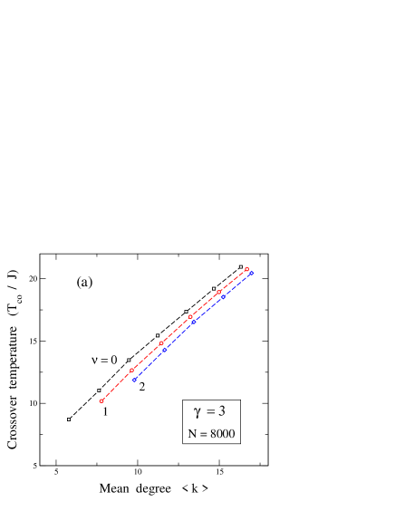
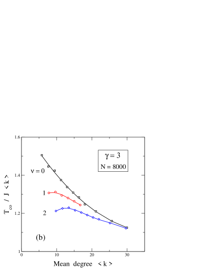
Figure 7: (a) Crossover temperature as a function of the mean degree $\langle k\rangle$, for networks with $\gamma=3$ and $N$ = 8000 nodes. Symbols represent results for three $\nu$ values: 0 (squares), 1 (circles), and 2 (diamonds). The data shown were obtained for networks with several minimum degrees, $k_{0}\geq 3$. (b) Ratio $T_{\rm co}/J\langle k\rangle$ vs $\langle k\rangle$ for the same kind of networks as in (a). Lines are guides to the eye.

Given the increase in crossover temperature for rising system size $N$, it is worthwhile analyzing the dependence of $T_{\rm co}$ on the minimum degree $k_{0}$. In fact, given the parameters $\gamma$ and $\nu$, $k_{0}$ controls the mean degree $\langle k\rangle$ of our networks. In Fig. 7(a) we display results for $T_{\rm co}/J$ for an exponent $\gamma=3$ and triangle density $\nu$ = 0, 1, and 2. In all cases, the networks included $N$ = 8000 nodes. As expected, for a given value of $\nu$, the crossover temperature increases as $\langle k\rangle$ (or $k_{0}$) is raised. Moreover, the line giving the dependence of $T_{\rm co}$ on $\langle k\rangle$ shifts downwards for rising $\nu$. In view of Eq. (17), this can be interpreted from a decrease in the ratio $\langle k^{2}\rangle/\langle k\rangle$ for networks with constant size and increasing triangle density $\nu$. Note, however, that the dependence of $T_{\rm co}$ on $\langle k\rangle$ is not strictly linear for fixed $N$, as predicted by Eq. (21). This is a finite-size effect, since this equation corresponds to the asymptotic limit, valid in the large-$N$ regime, so that for $N$ = 8000 such an effect is still clearly appreciable in the results shown in Fig. 7(a). This can be further visualized in Fig. 7(b), where we present the ratio $T_{\rm co}/(J\langle k\rangle)$ for the same data as in panel (a). Values of this ratio corresponding to different triangle densities $\nu$ converge one to the other as the mean degree increases.

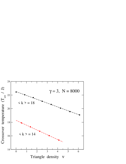
Figure 8: Crossover temperature $T_{\rm co}/J$ for scale-free networks with $\gamma=3$ and $N$ = 8000 nodes, as a function of the triangle density $\nu$. Each set of data corresponds to a fixed value of the mean degree: $\langle k\rangle$ = 14 (circles) and $\langle k\rangle$ = 18 (squares). Dashed lines are least-square fits to the data points.

For networks with a given size $N$, it is interesting to analyze the dependence of $T_{\rm co}$ on the parameter $\nu$ for a fixed value of the mean degree $\langle k\rangle$. Since $\langle k\rangle=\langle s\rangle+2\nu$, one can obtain networks with given $\langle k\rangle$ by simultaneously changing $\langle s\rangle$ and $\nu$. In the actual implementations, we varied the minimum degree $k_{0}$, which defines a mean value $\langle s\rangle$, and then we took $\nu=(\langle k\rangle-\langle s\rangle)/2$, $\langle k\rangle$ being the required mean degree of the clustered networks. In Fig. 8 we show the dependence of $T_{\rm co}$ on the triangle density $\nu$ for $\langle k\rangle$ = 14 and 18. As expected from the data shown in Fig. 7, $T_{\rm co}$ decreases for rising $\nu$, and this dependence turns out to be linear in both cases considered here. The slope of this line is more negative for $\langle k\rangle$ = 14 than for $\langle k\rangle$ = 18. In fact, we found: $dT_{\rm co}/d\nu$ = –0.70 $J$ and –0.56 $J$ for $\langle k\rangle$ = 14 and 18, respectively.

This means that for networks with given size $N$ and mean degree $\langle k\rangle$, including triangles in the networks (i.e., increasing the triangle density $\nu$) reduces the crossover temperature $T_{\rm co}$. The reason for this is the following. To have a constant $\langle k\rangle$ when changing $\nu$ for a given $\gamma$ ($\gamma=3$ here), one needs a minimum degree $k_{0}=\langle k\rangle/2-\nu$ [see Eq. (4)], so that a rise of $\nu$ is associated to a decrease in $k_{0}$. This causes a reduction of $\langle k^{2}\rangle$, and therefore the temperature $T_{\rm co}$ decreases.

In other words, adding triangles to a network changes the degree distribution $P(k)$ itself, apart from introducing clustering into the network. When one includes triangles ($\nu$ increases) without changing the other parameters defining the networks (i.e., $N$, $k_{0}$, $\gamma$), one finds a clear increase in $T_{\rm co}$, as shown in Fig. 6. However, if one changes $\nu$ subject to some particular restriction on the degree distribution, such as keeping constant the mean value $\langle k\rangle$, one may find other types of dependence of $T_{\rm co}$ on $\nu$ (as the decrease shown in Fig. 8).

This suggests that a relevant point here is a comparison between clustered and unclustered networks with the same degree distribution $P(k)$. This will give insight into the ‘direct’ effect of clustering on the critical properties of the Ising model. As commented above, the distribution $P(k)$, as well as Eq. (11) predicting the crossover temperature, do not include any information on the clustering present in the considered networks, but only on the degrees (connectivity) of the nodes. Thus, a natural question is the relevance of the difference between the crossover temperature corresponding to networks with the same size $N$ and degree distribution $P(k)$, but including triangles or not. We have seen above that in the case $\gamma>3$ both types of networks have the same transition temperature $T_{c}$, which agrees with Eq. (11). This is not clear, however, for $\gamma=3$. To clarify this point we have generated networks with the same $P(k)$ as those studied above for different $\nu$ values, but without including triangles. In this case, we used the distribution $P(k)$ to define the set of degrees $\{s_{i}\}_{i=1}^{N}$, employed to build up the networks ($k_{i}=s_{i}$ for all $i$).

Figure 9: Crossover temperature as a function of system size $N$ for networks with $\gamma=3$, $\nu=2$, and minimum degree $k_{0}=3$. Circles and squares represent results of MC simulation for networks with and without triangles, but with the same degree distribution $P(k)$. Error bars are less than the symbol size. The solid line is the analytical prediction, Eq. (11), obtained from the mean values $\langle k\rangle$ and $\langle k^{2}\rangle$.

In Fig. 9 we present the temperature $T_{\rm co}$ as a function of system size for networks with (circles) and without (squares) triangles, as derived from our MC simulations. Clustered networks were generated with $\gamma=3$, $\nu=2$, minimum degree $k_{0}=3$, and several sizes up to $N=2\times 10^{5}$ nodes. Unclustered networks were built up with the same distribution $P(k)$ as the clustered ones. The results presented in Fig. 9, indicate first that clustering increases $T_{\rm co}$, and this increase becomes more important for larger system size. As discussed above, for the clustered networks we find a dependence $T_{\rm co}/J=A\ln N+B$, with a slope $A$ close to unity ($A=1.09$). We have also plotted the crossover temperature predicted by Eq. (11), which takes only into account the average values $\langle k\rangle$ and $\langle k^{2}\rangle$ (solid line). A linear dependence on $\ln N$ is also found in this case, but with a smaller coefficient $A=0.87$. In fact, this line crosses with that derived from MC simulations for a system size $N\approx 10^{5}$.

Looking at the size dependence of the crossover temperature for unclustered networks shown in Fig. 9 (dashed-dotted line), we observe that for $N<10^{4}$ the curve $T_{\rm co}(N)$ found for these networks is parallel (slightly below) to that found for clustered networks (dashed line). For larger system sizes, the dashed-dotted curve becomes parallel to that corresponding to the analytical model (solid line).

For a given system size, clustered networks display a crossover temperature $T_{\rm co}$ larger than unclustered networks with the same degree distribution $P(k)$. This means that clustering (triangles in this case) favors an increase in $T_{\rm co}$, i.e. the FM phase is stable in a broader temperature range. This has been already observed in the results shown in Fig. 6, but in that case the difference between clustered and unclustered networks was larger, due to the inclusion of triangles for $\nu>0$, which changed the actual degree distribution $P(k)$ with respect to the case $\nu=0$.

The result for unclustered networks (no triangles) shown in Fig. 9 converges to the analytical data given by $T_{\rm co}\sim AJ\ln N$, with $A$ = 0.87, as expected from the asymptotic limit for Eq. (11). For large system size, the behavior of unclustered networks is in this respect controlled by nodes with large degree. Given that the effective degree cutoff scales as $k_{\rm cut}\sim N^{1/2}$ [see Eq. (33)], nodes with large $k$ appear progressively as $N$ is increased. Thus, the presence of nodes with high degree favors ferromagnetic correlations in clustered networks, and therefore an increase in the crossover temperature $T_{\rm co}$.

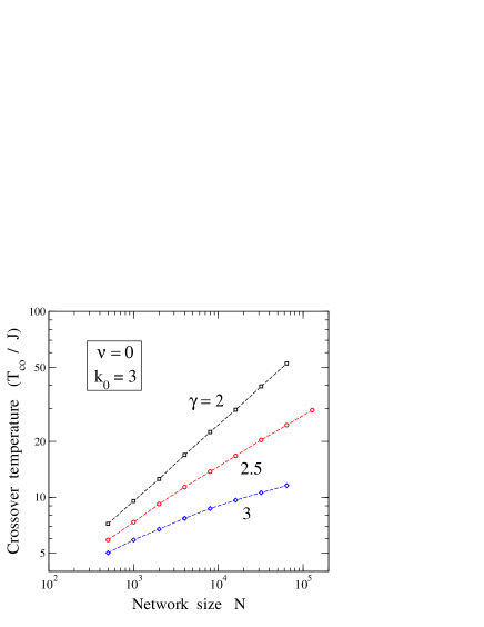
Figure 10: Crossover temperature $T_{\rm co}/J$ for scale-free networks with $\nu=0$ and $k_{0}=3$, as a function of system size $N$ in a logarithmic plot. Symbols represent results for three values of the parameter $\gamma$: 2 (squares), 2.5 (circles), and 3 (diamonds). Error bars are less than the symbol size. Lines are guides to the eye.

IV.3 Case $\gamma<3$

As commented above, for $\gamma<3$ it is known that correlations between degrees of adjacent nodes appear in scale-free networks when no multiple and self-connections are allowed, unless one takes a degree cutoff $k_{\rm cut}\lesssim\sqrt{N}$ Catanzaro et al. (2005). For this reason, we generated clustered and unclustered networks with $\gamma<3$ assuming a cutoff $k_{\rm cut}=\sqrt{N}$. This means that in this case Eq. (5) does not apply. With a calculation similar to that presented in the Appendix, one finds in this case for unclustered scale-free networks ($\nu=0$):

$$\langle k^{2}\rangle\approx\frac{\gamma-1}{3-\gamma}\,k_{0}^{\gamma-1}\,N^{(3-\gamma)/2}\;.$$ (22)

For $2<\gamma<3$, one has for the mean degree:

$$\langle k\rangle\approx k_{0}\,\frac{\gamma-1}{\gamma-2}\;,$$ (23)

as in Eq. (3). For $\gamma=2$, $\langle k\rangle$ diverges to infinity in the large-size limit as

$$\langle k\rangle\approx\frac{1}{2}\,k_{0}\,\ln N\;.$$ (24)

Thus, one expects a size-dependent crossover temperature

$$\frac{T_{\rm co}}{J}\approx\frac{\langle k^{2}\rangle}{\langle k\rangle}\approx\frac{\gamma-2}{3-\gamma}\,k_{0}^{\gamma-2}\,N^{(3-\gamma)/2}$$ (25)

for $2<\gamma<3$, and

$$\frac{T_{\rm co}}{J}\approx 2\,\frac{\sqrt{N}}{\ln N}$$ (26)

for $\gamma=2$.

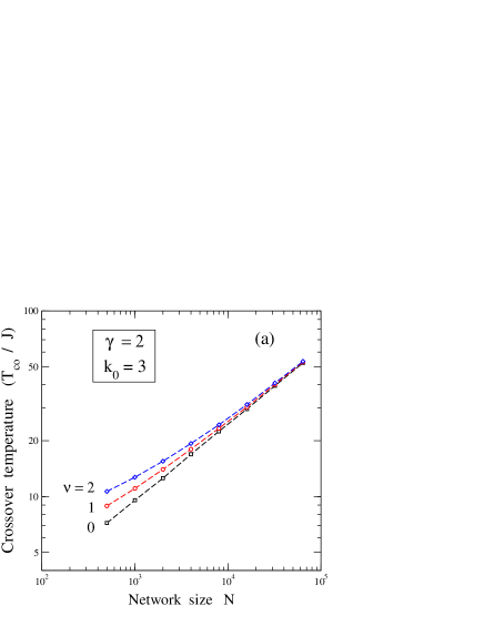
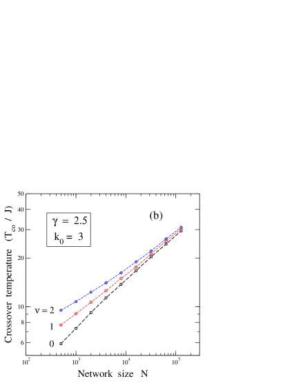
Figure 11: Crossover temperature $T_{\rm co}/J$ as a function of system size $N$ for scale-free networks with minimum degree $k_{0}$ = 3, and three values of the triangle density $\nu$: 0 (squares), 1 (circles), and 2 (diamonds). (a) Networks with $\gamma=2$; (b) networks with $\gamma=2.5$. Lines are guides to the eye.

We first present results for unclustered networks ($\nu=0$). In Fig. 10 we show the temperature $T_{\rm co}$ as a function of system size $N$ for three values of $\gamma$ in a logarithmic plot, as derived from our MC simulations for networks with minimum degree $k_{0}=3$. The exponent $\gamma$ increases from top to bottom: $\gamma$ = 2, 2.5, and 3. For a given system size, $T_{\rm co}$ decreases as $\gamma$ rises. This is a consequence of a decrease in the ratio $\langle k^{2}\rangle/\langle k\rangle$ for increasing $\gamma$, which causes a reduction in $T_{\rm co}$, as predicted by Eq. (25), where the term $N^{(3-\gamma)/2}$ dominates for large $N$.

For networks with $\gamma<3$ and large-enough size, $\log T_{\rm co}$ derived from the MC simulations is found to display a linear dependence on $\log N$, as expected for a crossover temperature diverging as a power of the system size $T_{\rm co}\sim N^{z}$ with an exponent $z$ dependent on the parameter $\gamma$ Herrero (2004). Such a linear dependence is obtained for system sizes $N\gtrsim N_{0}$, the size $N_{0}$ increasing with the exponent $\gamma$ and eventually diverging for $\gamma\to 3$, for which $T_{\rm co}\sim\ln N$ is expected (see Fig. 6). According to Eq. (25), one expects $z=(3-\gamma)/2$. In fact, for $\gamma=2.5$ we find $z=0.27$ from a fit to the data points corresponding to networks with $N>10^{4}$. This value of $z$ could further decrease for larger system sizes, what is compatible with the exponent $z=0.25$ expected from Eq. (25).

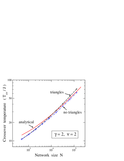
Figure 12: Crossover temperature as a function of system size $N$ for networks with $\gamma=2$, $\nu=2$, and minimum degree $k_{0}=3$. Circles and squares represent results of MC simulations for networks with and without triangles, respectively, but with the same degree distribution $P(k)$. Error bars are less than the symbol size. The solid line indicates the result derived from $\langle k\rangle$ and $\langle k^{2}\rangle$ by using Eq. (11).

We note that the degree cutoff is relevant for the size-dependence of the crossover temperature. Thus, the cutoff employed here for networks with $\gamma<3$ ($k_{\rm cut}=\sqrt{N}$) yields an exponent $z=(3-\gamma)/2$, to be compared with $z=(3-\gamma)/(\gamma-1)$, given by the “natural” cutoff in Eqs. (5) and (33) [see Refs. Dorogovtsev et al., 2002; Iglói and Turban, 2002; Herrero, 2004]. The latter cutoff is known to introduce undesired correlations in networks such as those considered here with $\gamma<3$, as commented above.

We now turn to clustered networks. In Fig. 11 we show the crossover temperature vs system size $N$ for networks with different triangle densities: $\nu$ = 0, 1, and 2. In panels (a) and (b) results are given for $\gamma$ = 2 and 2.5, respectively. For small network size, $T_{\rm co}$ appears to be higher for larger parameter $\nu$ in both cases. This difference, however, decreases as $N$ is increased, and for each value of $\gamma$ the results for different triangle densities $\nu$ converge one to the other. Thus, in the logarithmic plots of Fig. 11 differences between the crossover temperature for different $\nu$ values become irrelevant for system size $N\sim 10^{5}$.

Similarly to the case $\gamma=3$ presented in Sec. IV.B, for $\gamma<3$ it is also interesting to compare results for clustered and unclustered networks with the same degree distribution $P(k)$. In Fig. 12 we present the temperature $T_{\rm co}$ as a function of system size for networks with (circles) and without (squares) triangles, as derived from our MC simulations. Clustered networks were generated with $\gamma=2$, $\nu=2$, minimum degree $k_{0}=3$, and various system sizes. For $N<2000$ nodes, results for clustered and unclustered networks coincide one with the other within statistical noise. For $N>2000$, both sets of data progressively separate one from the other, so that the crossover temperature for clustered networks (including triangles) is larger than that corresponding to unclustered networks (no triangles). The solid line in Fig. 12 is the analytical prediction obtained from Eq. (11) by introducing the mean values $\langle k\rangle$ and $\langle k^{2}\rangle$ corresponding to the actual networks. We observe something similar to the case of $\gamma=3$ shown in Fig. 9. For large $N$, results of MC simulations for unclustered networks approach the analytical expectancy, lying below the solid line, whereas data for clustered networks become higher than the analytical prediction, and progressively deviate from the latter as system size $N$ is increased.

As for the case $\gamma=3$, we conclude that clustering favors a stabilization of the FM phase vs the PM one, hence increasing the crossover temperature $T_{\rm co}$. This becomes more noticeable for larger network size, where nodes with higher degree progressively appear.

V Summary

We have studied the FM-PM transition for the Ising model in clustered scale-free networks by means of Monte Carlo simulations, and the results were compared with those found for unclustered networks. Our results can be classified into two different regions, as a function of the exponent $\gamma$ defining the power-law for the degree distribution in scale-free networks.

For $\gamma>3$, we find in all cases a well-defined transition temperature $T_{c}$ in the thermodynamic limit, in agreement with earlier analytical calculations and MC simulations. This refers equally to clustered and unclustered networks. Adding motifs (triangles in our case) to the networks causes an increase in the transition temperature, as a consequence of the associated change in the degree distribution $P(k)$, and in particular in the mean values $\langle k\rangle$ and $\langle k^{2}\rangle$. However, for clustered and unclustered networks with the same degree distribution $P(k)$, one finds no difference in $T_{c}$, which coincides with that predicted by analytical calculations [Eq. (11)]. This conclusion agrees with that drawn in Ref. Yoon et al., 2011, where the addition of motifs was found to increase the transition temperature, without changing the critical behavior.

For networks with $\gamma\leq 3$, the situation is different. In this case, the crossover temperature $T_{\rm co}$ increases with system size $N$. For $\gamma=3$ we found $T_{\rm co}\sim J\ln N$, and for $\gamma<3$ we obtained $T_{\rm co}\sim JN^{z}$, with an exponent $z=(3-\gamma)/2$. Comparing clustered and unclustered networks, the conclusions obtained for $\gamma\leq 3$ differ from those found for $\gamma>3$.

For $\gamma\leq 3$, $T_{\rm co}$ is similar for clustered and unclustered networks with the same degree distribution $P(k)$, when one considers small network sizes ($N\lesssim 10^{3}$). This behavior changes for larger networks, and the crossover temperature $T_{\rm co}$ of clustered networks becomes progressively larger than that corresponding to the unclustered ones. Thus, we find that FM correlations are favored by including triangles in the networks, in particular in the presence of nodes with large degree $k$.

It is important to note that this conclusion refers to a comparison of clustered and unclustered networks with the same degree distribution $P(k)$. Caution should be taken when comparing results for networks with different degree distributions. Thus, when triangles are added on a network with a given distribution of links, the crossover temperature $T_{\rm co}$ increases [see Fig. 6], but in this case the rise in $T_{\rm co}$ is mainly due to the change in $P(k)$ caused by the inclusion of triangles. However, for clustered networks with the same exponent $\gamma$ (large-degree tail) and mean degree $\langle k\rangle$, an increase in triangle density $\nu$ causes a decrease in $T_{\rm co}$ [see Fig. 8], as a consequence of the associated variation in the distribution $P(k)$, and in particular in the mean value $\langle k^{2}\rangle$.

We also note that results for unclustered or clustered scale-free networks may differ when different degree cutoffs are employed, especially for $\gamma<3$, as the dependence of their properties on system size can be appreciable. This applies, in particular, to the scaling of the crossover temperature $T_{\rm co}$ on $N$ for large system size. To avoid correlations between degrees of adjacent nodes, we have employed here for power-law distributions a degree cutoff $k_{\rm cut}=N^{1/2}$. However, for clustered networks the presence of triangles introduces degree correlations.

Other distributions different from the short-tailed Poisson-type introduced here for the triangles, could be considered to change more dramatically the long-degree tail of the overall degree distribution $P(k)$. For example, a power-law distribution for the triangles (with an exponent $\gamma^{\prime}$) may give rise to an interesting competition between the exponents of both distributions (for single links and triangles), which could change the critical behavior of the Ising model on such networks as compared to those discussed here.

Appendix A Finite-size effects on degree distributions

Here we present some expressions related to finite-size effects in scale-free networks. We assume a degree distribution $P_{\rm sf}(k)$ defined as

$$P_{\rm sf}(k)=\left\{\begin{array}[]{ll}n\,k^{-\gamma},&{\rm for}\,k\geq k_{0}\\ 0,&{\rm for}\,k<k_{0}\end{array}\right.$$ (27)

with $\gamma>2$ and $n$ a normalization constant.

Due to the finite network size $N$, an effective cutoff $k_{\rm cut}$ appears for the degree distribution in these networks Dorogovtsev et al. (2002); Iglói and Turban (2002). This cutoff is such that $\sum_{k_{\rm cut}}^{\infty}P_{\rm sf}(k)\sim 1/N$, indicating that the number of nodes with $k>k_{\rm cut}$ is expected to be on the order of unity. For concreteness, we write

$$\sum_{k_{\rm cut}}^{\infty}P_{\rm sf}(k)=\frac{c}{N}$$ (28)

with $c={\cal O}(1)$. Replacing the sum by an integral, we find

$$\sum_{k_{\rm cut}}^{\infty}P_{\rm sf}(k)\approx\frac{n}{\gamma-1}\,k_{\rm cut}^{1-\gamma}\;.$$ (29)

For $c/N\ll 1$, one has for the normalization condition:

$$1=\frac{c}{N}+\sum_{k_{0}}^{k_{\rm cut}}P_{\rm sf}(k)\approx\frac{n}{\gamma-1}\,(k_{0}^{1-\gamma}-k_{\rm cut}^{1-\gamma})\;.$$ (30)

Then, the normalization constant $n$ is:

$$n=\frac{\gamma-1}{k_{0}^{1-\gamma}-k_{\rm cut}^{1-\gamma}}\approx(\gamma-1)\,k_{0}^{\gamma-1}\,.$$ (31)

Combining Eqs. (28), (29), and (31) one finds

$$\frac{N}{c}=\left(\frac{k_{\rm cut}}{k_{0}}\right)^{\gamma-1}-1\;,$$ (32)

and for $k_{\rm cut}\gg k_{0}$:

$$k_{\rm cut}\approx k_{0}\left(\frac{N}{c}\right)^{\frac{1}{\gamma-1}}\,,$$ (33)

so that $k_{\rm cut}\sim\,N^{1/(\gamma-1)}$, as in Refs. Dorogovtsev et al., 2002; Iglói and Turban, 2002. Considering this cutoff, one has for the mean degree

$$\langle k\rangle=\sum_{k_{0}}^{k_{\rm cut}}k\,P_{\rm sf}(k)=\frac{\gamma-1}{\gamma-2}\,\,\frac{k_{\rm cut}^{2-\gamma}-k_{0}^{2-\gamma}}{k_{\rm cut}^{1-\gamma}-k_{0}^{1-\gamma}}$$ (34)

which gives, using Eq. (33):

$$\langle k\rangle\approx\langle k\rangle_{\infty}\,\frac{\left(\frac{c}{N}\right)^{\frac{\gamma-2}{\gamma-1}}-1}{\frac{c}{N}-1}$$ (35)

with $\langle k\rangle_{\infty}\approx k_{0}(\gamma-1)/(\gamma-2)$. Thus, we find for the mean degree $\langle k\rangle$:

$$\langle k\rangle\approx\langle k\rangle_{\infty}\left[1-\left(\frac{c}{N}\right)^{\frac{\gamma-2}{\gamma-1}}+{\cal O}\left(\frac{1}{N}\right)\right]\;.$$ (36)

A similar calculation can be carried out to estimate finite-size effects on $\langle k^{2}\rangle$ for scale-free networks. For $\gamma>3$, we find:

$$\langle k^{2}\rangle\approx\langle k^{2}\rangle_{\infty}\left[1-\left(\frac{c}{N}\right)^{\frac{\gamma-3}{\gamma-1}}+{\cal O}\left(\frac{1}{N}\right)\right]$$ (37)

with $\langle k^{2}\rangle_{\infty}\approx k_{0}^{2}\,(\gamma-1)/(\gamma-3)$.

For $\gamma=3$, we have

$$\langle k^{2}\rangle=n\sum_{k_{0}}^{k_{\rm cut}}\frac{1}{k}\approx\frac{2}{k_{0}^{-2}-k_{\rm cut}^{-2}}\,\ln\frac{k_{\rm cut}}{k_{0}}$$ (38)

and using Eq. (33), we obtain for $k_{\rm cut}\gg k_{0}$:

$$\langle k^{2}\rangle=k_{0}^{2}\,\ln N+{\cal O}\left(1\right)$$ (39)

For $\gamma<3$ a strict cutoff $k_{\rm cut}=\sqrt{N}$ has been introduced in the networks discussed in the present paper, in order to avoid undesired correlations Catanzaro et al. (2005). Thus, the equations given in this appendix do not apply to the actual networks discussed in Sec. IV.C.

References

- Strogatz (2001) S. H. Strogatz, Nature 410, 268 (2001).
- Albert and Barabási (2002) R. Albert and A. L. Barabási, Rev. Mod. Phys. 74, 47 (2002).
- Dorogovtsev and Mendes (2003) S. N. Dorogovtsev and J. F. F. Mendes, Evolution of Networks: From Biological Nets to the Internet and WWW (Oxford University, Oxford, 2003).
- Newman (2010) M. E. J. Newman, Networks. An Introduction (Oxford University Press, New York, 2010).
- Cohen and Havlin (2010) R. Cohen and S. Havlin, Complex networks. Structure, robustness and function (Cambridge University Press, Cambridge, 2010).
- Watts and Strogatz (1998) D. J. Watts and S. H. Strogatz, Nature 393, 440 (1998).
- Barabási and Albert (1999) A. L. Barabási and R. Albert, Science 286, 509 (1999).
- Herrero (2002a) C. P. Herrero, Phys. Rev. E 66, 046126 (2002a).
- Pandit and Amritkar (2001) S. A. Pandit and R. E. Amritkar, Phys. Rev. E 63, 041104 (2001).
- Lahtinen et al. (2001) J. Lahtinen, J. Kertész, and K. Kaski, Phys. Rev. E 64, 057105 (2001).
- Candia (2007) J. Candia, Phys. Rev. E 75, 026110 (2007).
- Moore and Newman (2000) C. Moore and M. E. J. Newman, Phys. Rev. E 61, 5678 (2000).
- Kuperman and Abramson (2001) M. Kuperman and G. Abramson, Phys. Rev. Lett. 86, 2909 (2001).
- Newman and Watts (1999) M. E. J. Newman and D. J. Watts, Phys. Rev. E 60, 7332 (1999).
- Barrat and Weigt (2000) A. Barrat and M. Weigt, Eur. Phys. J. B 13, 547 (2000).
- Leone et al. (2002) M. Leone, A. Vázquez, A. Vespignani, and R. Zecchina, Eur. Phys. J. B 28, 191 (2002).
- Herrero (2002b) C. P. Herrero, Phys. Rev. E 65, 066110 (2002b).
- Castellano et al. (2005) C. Castellano, V. Loreto, A. Barrat, F. Cecconi, and D. Parisi, Phys. Rev. E 71, 066107 (2005).
- Dorogovtsev et al. (2008) S. N. Dorogovtsev, A. V. Goltsev, and J. F. F. Mendes, Rev. Mod. Phys. 80, 1275 (2008).
- Herrero (2009a) C. P. Herrero, J. Phys. A: Math. Gen. 42, 415102 (2009a).
- Ostilli et al. (2011) M. Ostilli, A. L. Ferreira, and J. F. F. Mendes, Phys. Rev. E 83, 061149 (2011).
- Dorogovtsev and Mendes (2002) S. N. Dorogovtsev and J. F. F. Mendes, Adv. Phys. 51, 1079 (2002).
- Goh et al. (2002) K. I. Goh, E. S. Oh, H. Jeong, B. Kahng, and D. Kim, Proc. Natl. Acad. Sci. USA 99, 12583 (2002).
- Siganos et al. (2003) G. Siganos, M. Faloutsos, P. Faloutsos, and C. Faloutsos, IEEE ACM Trans. Netw. 11, 514 (2003).
- Albert et al. (1999) R. Albert, H. Jeong, and A. L. Barabási, Nature 401, 130 (1999).
- Jeong et al. (2001) H. Jeong, S. P. Mason, A. L. Barabási, and Z. N. Oltvai, Nature 411, 41 (2001).
- Newman (2001) M. E. J. Newman, Proc. Natl. Acad. Sci. USA 98, 404 (2001).
- Krapivsky et al. (2000) P. L. Krapivsky, S. Redner, and F. Leyvraz, Phys. Rev. Lett. 85, 4629 (2000).
- Hébert-Dufresne et al. (2011) L. Hébert-Dufresne, A. Allard, V. Marceau, P.-A. Noël, and L. J. Dubé, Phys. Rev. Lett. 107, 158702 (2011).
- Bogacz et al. (2006) L. Bogacz, Z. Burda, and B. Waclaw, Physica A 366, 587 (2006).
- Holme and Kim (2002) P. Holme and B. J. Kim, Phys. Rev. E 65, 026107 (2002).
- Klemm and Eguiluz (2002) K. Klemm and V. M. Eguiluz, Phys. Rev. E 65, 036123 (2002).
- Serrano and Boguñá (2005) M. A. Serrano and M. Boguñá, Phys. Rev. E 72, 036133 (2005).
- Newman (2009) M. E. J. Newman, Phys. Rev. Lett. 103, 058701 (2009).
- Miller (2009) J. C. Miller, Phys. Rev. E 80, 020901 (2009).
- Dorogovtsev et al. (2002) S. N. Dorogovtsev, A. V. Goltsev, and J. F. F. Mendes, Phys. Rev. E 66, 016104 (2002).
- Iglói and Turban (2002) F. Iglói and L. Turban, Phys. Rev. E 66, 036140 (2002).
- Herrero (2004) C. P. Herrero, Phys. Rev. E 69, 067109 (2004).
- Dommers et al. (2010) S. Dommers, C. Giardina, and R. van der Hofstad, J. Stat. Phys. 141, 638 (2010).
- Menche et al. (2011) J. Menche, A. Valleriani, and R. Lipowsky, Phys. Rev. E 83, 061129 (2011).
- Bartolozzi et al. (2006) M. Bartolozzi, T. Surungan, D. B. Leinweber, and A. G. Williams, Phys. Rev. B 73, 224419 (2006).
- Herrero (2009b) C. P. Herrero, Eur. Phys. J. B 70, 435 (2009b).
- Gleeson (2009) J. P. Gleeson, Phys. Rev. E 80, 036107 (2009).
- Gleeson et al. (2010) J. P. Gleeson, S. Melnik, and A. Hackett, Phys. Rev. E 81, 066114 (2010).
- Karrer and Newman (2010) B. Karrer and M. E. J. Newman, Phys. Rev. E 82, 066118 (2010).
- Allard et al. (2012) A. Allard, L. Hebert-Dufresne, P.-A. Noel, V. Marceau, and L. J. Dube, J. Phys. A: Math. Theor. 45, 405005 (2012).
- Wang et al. (2012) B. Wang, L. Cao, H. Suzuki, and K. Aihara, J. Theor. Biol. 304, 121 (2012).
- Molina and Stone (2012) C. Molina and L. Stone, J. Theor. Biol. 315, 110 (2012).
- Hebert-Dufresne et al. (2010) L. Hebert-Dufresne, P.-A. Noel, V. Marceau, A. Allard, and L. J. Dube, Phys. Rev. E 82, 036115 (2010).
- Melnik et al. (2011) S. Melnik, A. Hackett, M. A. Porter, P. J. Mucha, and J. P. Gleeson, Phys. Rev. E 83, 036112 (2011).
- Yoon et al. (2011) S. Yoon, A. V. Goltsev, S. N. Dorogovtsev, and J. F. F. Mendes, Phys. Rev. E 84, 041144 (2011).
- Newman (2005) M. E. J. Newman, Contemp. Phys. 46, 323 (2005).
- Catanzaro et al. (2005) M. Catanzaro, M. Boguñá, and R. Pastor-Satorras, Phys. Rev. E 71, 027103 (2005).
- Binder and Heermann (2010) K. Binder and D. W. Heermann, Monte Carlo Simulation in Statistical Physics (Springer, Berlin, 2010), 5th ed.
- Herrero (2008) C. P. Herrero, Phys. Rev. E 77, 041102 (2008).
- Aleksiejuk et al. (2002) A. Aleksiejuk, J. A. Holyst, and D. Stauffer, Physica A 310, 260 (2002).
- Aleksiejuk-Fronczak (2002) A. Aleksiejuk-Fronczak, Int. J. Mod. Phys. C 13, 1415 (2002).