Spectral statistics of chaotic many-body systems

Abstract

We derive a trace formula that expresses the level density of chaotic many-body systems as a smooth term plus a sum over contributions associated to solutions of the nonlinear Schrödinger (or Gross-Pitaevski) equation. Our formula applies to bosonic systems with discretised positions, such as the Bose-Hubbard model, in the semiclassical limit as well as in the limit where the number of particles is taken to infinity. We use the trace formula to investigate the spectral statistics of these systems, by studying interference between solutions of the nonlinear Schrödinger equation. We show that in the limits taken the statistics of fully chaotic many-particle systems becomes universal and agrees with predictions from the Wigner-Dyson ensembles of random matrix theory. The conditions for Wigner-Dyson statistics involve a gap in the spectrum of the Frobenius-Perron operator, leaving the possibility of different statistics for systems with weaker chaotic properties.

1 Introduction

Feynman’s path integral (see e.g. [1]) provides a convenient way to represent the propagator of a quantum mechanical system, and an excellent starting point for semiclassical and related approximations. Prime examples are van Vleck’s approximation of the propagator of a quantum system as a sum over contributions of classical trajectories [2], and Gutzwiller’s seminal work [3] relating the energy spectrum of chaotic single-particle systems to periodic classical trajectories. These semiclassical methods provide one of the foundations of the field of quantum chaos [4, 5, 6]. For a many-particle system identifying the semiclassical limit is less obvious. A promising approach is to consider the path integral in second quantisation, running over different choices for the macroscopic wave function parameterised by position and time. One can show that in the semiclassical limit and in the limit where the number of particles $N$ is taken to infinity this path integral is dominated by stationary points of the action, corresponding to solutions of the nonlinear Schrödinger equation or Gross-Pitaevski equation. These solutions take on a role analogous to the one played by classical trajectories in the single-particle theory. However previous work usually focused either on studying the full problem in second quantisation or, as e.g. in nuclear dynamics [7], on one dominating solution to the Gross-Pitaevski equation [8, 9]. This does not exhaust the power of the approximation. In particular keeping the sum over different solutions of the Gross-Pitaevski equation allows to account for crucial interference effects between such solutions. An approach where the semiclassical propagator of bosonic many-particle systems was used to study these effects was pioneered in [10] for coherent backscattering, see also [11] for applications to fermionic systems.

In the present paper we will focus on a further fundamental problem for which the interference between stationary points of second quantised path integrals is of vital importance: the statistics of the energy levels of many-body systems. To do so we will first derive an approximation of the level density in terms of stationary points of the action, and then study the interference between these points. To our knowledge the consequences of interference effects for many-body spectral statistics have not yet been investigated explicitly. We will see that this statistics depends crucially on the dynamics generated by the Gross-Pitaevski equation. If the dynamics is fully chaotic (in the sense to be specified below) the statistics in the limits considered becomes universal, and agrees with predictions from random-matrix theory (RMT). These predictions entail, for instance, a repulsion between the energy levels.

This universal behaviour mirrors the behaviour of chaotic single-particle systems studied in the semiclassical limit. For such systems spectral statistics faithful to random matrix theory was conjectured in [12], and a semiclassical explanation was developed in [13, 14, 15, 16, 17, 18]. This explanation is based on Gutzwiller’s trace formula [3, 4, 5, 19]

$$d(E)\approx\bar{d}(E)+\frac{1}{\pi\hbar}{\rm Re}\sum_{p}A_{p}e^{iS_{p}/\hbar}$$ (1)

which expresses the level density as a smooth term $\bar{d}(E)$ plus fluctuations associated to classical periodic orbits $p$ (with energy $E$) of the system. Here $S_{p}$ is the reduced action of the orbit given by $S_{p}=\int\boldsymbol{p}(t)\cdot\boldsymbol{\dot{q}}(t)dt$ where ${\boldsymbol{q}}(t)$ denotes the vector of generalised coordinates and ${\boldsymbol{p}}(t)$ denotes the associated momentum. The amplitude $A_{p}=\frac{T_{p}^{\rm prim}e^{-i\mu_{p}\frac{\pi}{2}}}{\sqrt{|\det(M_{p}-\mathbb{I})}|}$ depends on the primitive period $T_{p}^{\rm prim}$, the so-called Maslov index $\mu_{p}$ and the stability matrix $M_{p}$ relating deviations in the end of the orbit $p$ to deviations in the beginning; $\mathbb{I}$ is a unit matrix. (Throughout this paper $\mathbb{I}$ will denote unit matrices with a subscript indicating their size if it is not clear from context.) Our first aim will be to generalise the trace formula to bosonic many-particle systems in second quantisation, with solutions of the Gross-Pitaevski equation taking the role of classical trajectories.

We will then use this result to investigate spectral statistics. An observable characterising spectral statistics is the two-point correlation function of the level density $d(E)=\sum_{j}\delta(E-E_{j})$ (where $E_{j}$ are the energy levels of the system). This correlation function is defined by

$$R(\epsilon)=\frac{1}{\bar{d}^{2}}\left\langle d\left(E+\frac{\epsilon}{2\pi\bar{d}}\right)d\left(E-\frac{\epsilon}{2\pi\bar{d}}\right)\right\rangle$$ (2)

where the average $\langle\ldots\rangle$ is taken over an interval of $E$ for which $\bar{d}$ can be taken constant as well as over a small range of $\epsilon$. Inserting the trace formula one obtains a double sum over solutions of the Gross-Pitaevski equation, and by taking into account interference between solutions we indeed recover statistics in agreement with RMT.

More precisely this agreement holds for the statistics inside appropriate subspectra defined by the symmetries of the problem; for many-body systems we have at least one symmetry, particle number conservation, requiring to consider subspectra associated to a fixed particle number. Further refinements (to be discussed below) arise in case of geometrical symmetries. The precise ensemble to be chosen depends on the behaviour of the system under time reversal. The most frequent case involves systems invariant under a time-reversal operator squaring to 1. In this case (assuming that there are no further symmetries) one has to use Wigner’s and Dyson’s Gaussian Orthogonal Ensemble (GOE), i.e. predictions for spectral statistics are obtained by modelling the Hamiltonian through a real symmetric matrix, and then averaging over all possible such matrices with a Gaussian weight. In the absence of time-reversal invariance one averages instead over the ensemble of Hermitian matrices with a Gaussian weight, the Gaussian Unitary Ensemble (GUE).

A paradigmatic example for the systems to be considered is the Bose-Hubbard model, a model with $L$ discrete sites (labelled by $k=0\ldots L-1$) accommodating bosonic particles. Denoting the creation and annihilation operators for particles at these sites by $\hat{a}_{k}^{\dagger}$ and $\hat{a}_{k}$ the second-quantised Hamiltonian can be written as

$$\hat{H}=-\frac{J}{2}\sum_{k}(\hat{a}^{\dagger}_{k+1}\hat{a}_{k}+\hat{a}_{k}^{\dagger}\hat{a}_{k+1})+\frac{U}{2}\sum_{k}(\hat{a}_{k}^{\dagger})^{2}\hat{a}_{k}^{2}$$ (3)

describing hopping between the sites as well as interaction between particles on the same site. One can consider periodic boundary conditions and set $\hat{a}_{L}=\hat{a}_{0}$, $\hat{a}^{\dagger}_{L}=\hat{a}_{0}^{\dagger}$. More generally we are interested in discrete bosonic many-body Hamiltonians that are of the form

$$\hat{H}=\sum_{kl}h_{kl}\hat{a}_{k}^{\dagger}\hat{a}_{l}+\sum_{klmn}U_{klmn}\hat{a}_{k}^{\dagger}\hat{a}_{l}^{\dagger}\hat{a}_{m}\hat{a}_{n}$$ (4)

or have even higher-order interactions; here real coefficients imply time-reversal invariance.

A crucial requirement is that the underlying ‘classical dynamics’ is chaotic. This dynamics is obtained by replacing the creation and annihilation operators by mutually complex conjugate time dependent variables $\psi_{k}^{*}$, $\psi_{k}$ where $\boldsymbol{\psi}=(\psi_{0},\psi_{1},\ldots)$ can be interpreted as a macroscopic wave function and $\psi_{k}$ as its value at site $k$. As $\hat{N}=\sum_{k}\hat{a}_{k}^{\dagger}\hat{a}_{k}$ is the particle number operator, the macroscopic wave function is normalised to have $\sum_{k}|\psi_{k}|^{2}=N$ where $N$ is the particle number. The associated analogue of Hamilton’s equations for $\psi_{k}$ can be shown to read $i\hbar\dot{\psi}_{k}=\frac{\partial H}{\partial\psi_{k}^{*}}$ and takes the role of a discrete nonlinear Schrödinger equation.

We note that the ‘classical’ Hamiltonian entering into this equation depends on the ordering of operators. For the Bose-Hubbard model the normal-ordered Hamiltonian in (3) yields an interaction term $\frac{U}{2}\sum_{k}|\psi_{k}|^{4}$; however if the Hamiltonian is first brought to Weyl-ordered form (with all possible orderings of operators in a product contributing symmetrically) before replacing the operators by macroscopic wave functions one obtains $\frac{U}{2}\sum_{k}(|\psi_{k}|^{4}-2|\psi_{k}|^{2}+\frac{1}{2})$.

For the Bose-Hubbard model the dynamics generated by the discrete nonlinear Schrödinger equation has been found to be mainly chaotic (with chaotic regions of phase space dominating compared to regular ones) in the case of several sites and comparable hopping and interaction terms [20]. In the same regime, numerical studies suggest spectral statistics in line with the GOE [21, 22]; see also [23] for fermionic systems.

To explain the observed faithfulness to RMT, we follow a semiclassical approach inspired by single-body spectral statistics as well as [10]. Our first aim is to derive a trace formula for second quantised Bose-Hubbard-like systems. This will be done in Sect.$~{}2$, after a brief reminder of the corresponding derivation for one-body chaotic systems. Special emphasis is placed on the treatment of conserved quantities. In Sect.$~{}3$ it is demonstrated how the obtained trace formula can be used in order to predict the spectral statistics of the system, especially the $2-$point correlation function. We explain in detail how to generalise the approach previously used for one-body chaotic systems in first quantisation, and we discuss the range of validity of this approach. In Sect.$~{}4$ the consequences of discrete symmetries of chaotic many-body system, in particular for Bose Hubbard model are investigated. In Sect.$~{}5$ we present numerical results supporting our claims. Some more technical details of the derivation are put in two appendices.

2 Trace formula

2.1 Trace formula for single-body systems

In order to prepare our derivation of a trace formula for bosonic many-particle systems, we want to briefly review the calculation leading to the trace formula for single-body systems. We refer to [4, 5, 6, 24, 25] for further details.

The level density can be accessed from the trace of the time evolution operator $e^{-\frac{i}{\hbar}\hat{H}t}$ via

$$d(E)={\rm tr}\,\delta(E-\hat{H})=\frac{1}{\pi\hbar}{\rm Im}\,i\int_{0}^{\infty}dt\,e^{\frac{i}{\hbar}(E+i0)t}\,{\rm tr}\,e^{-\frac{i}{\hbar}\hat{H}t}\ ,$$ (5)

where an infinitesimal positive imaginary part has been added to the energy to ensure convergence. The trace of the time evolution operator can itself be expressed as a path integral over phase space trajectories $(\boldsymbol{q}(t),\boldsymbol{p}(t))$

$$\,{\rm tr}\,e^{-\frac{i}{\hbar}\hat{H}t}=\int D[\boldsymbol{q},\boldsymbol{p}]e^{iR[\boldsymbol{q},\boldsymbol{p}]/\hbar},$$ (6)

where the action weighting each path is determined by the classical Hamiltonian $H$ as

$$R[\boldsymbol{q},\boldsymbol{p}]=\int_{0}^{t}dt^{\prime}\left({\boldsymbol{p}(t^{\prime})}\cdot\dot{\boldsymbol{q}}(t^{\prime})-H(\boldsymbol{q}(t^{\prime}),\boldsymbol{p}(t^{\prime}))\right).$$ (7)

Now we are interested in an approximation of this path integral in the semiclassical limit, i.e., the limit of large quantum numbers implying that typical classical actions are much larger than $\hbar$; formally this limit is often denoted by $\hbar\to 0.$ In the semiclasssical limit the path integral is dominated by stationary points of the action, corresponding to periodic orbits that satisfy Hamilton’s equations of motion, and a stationary-phase approximation leads to a discrete sum over such periodic orbits. For chaotic dynamics, free from continuous symmetries, the periodic orbits are isolated but one has to take into account that each of them formally gives rise to a one-parameter family of stationary points distinguished by which phase-space point along the orbit is taken as the initial one associated to $t=0$. The Laplace transform in (5) can then be carried out in a further stationary-phase approximation and one obtains the trace formula

$$d(E)\approx\bar{d}(E)+\frac{1}{\pi\hbar}{\rm Re}\sum_{p}\frac{T_{p}^{\rm prim}e^{-i\mu_{p}\frac{\pi}{2}}}{\sqrt{|\det(M_{p}-\mathbb{I})}|}e^{iS_{p}/\hbar}$$ (8)

already shown earlier. Here the determinant and the phase factor involving the Maslov index arise from the Hessian matrix of the action entering the stationary-phase approximation, and the factor $T_{p}^{\rm prim}$ results from integration over different choices of initial points. The summand $\bar{d}(E)$ can be derived from a careful treatment of the lower limit of the time integral (5).

2.2 Path integral for many-particle systems

We now want to generalise the trace formula to many-particle systems in second quantisation, for the case of bosonic particles at discrete sites. In second quantisation it is natural to work in a basis of coherent states, i.e., normalised joint eigenstates of all annihilators $\hat{a}_{k}$ with eigenvalues $\psi_{k}$. Further differences from the single-particle setting arise from operator ordering as well as the conservation of the particle number.

Again we access the level density from the trace of the time evolution operator $e^{-\frac{i}{\hbar}\hat{H}t}$ using (5). For many-particle systems the latter trace is given by the path integral [26]

$$\,{\rm tr}\,e^{-\frac{i}{\hbar}\hat{H}t}=\int D[\boldsymbol{\psi},\boldsymbol{\psi}^{*}]e^{iR[\boldsymbol{\psi},\boldsymbol{\psi}^{*}]/\hbar}$$ (9)

over all macroscopic wave functions $\boldsymbol{\psi}(t^{\prime})$ that return to their initial value after time $t$. Here the action is

$$R[\boldsymbol{\psi},\boldsymbol{\psi}^{*}]=\int_{0}^{t}dt^{\prime}\left(-\frac{\hbar}{i}\boldsymbol{\psi}^{*}(t^{\prime})\cdot\dot{\boldsymbol{\psi}}(t^{\prime})-H(\boldsymbol{\psi}^{*}(t^{\prime}),\boldsymbol{\psi}(t^{\prime}))\right).$$ (10)

Eq. (9) is related to but somewhat simpler than the path integral for matrix elements of coherent state time evolution operator [27]; our use of ${\rm tr}\,e^{-\frac{i}{\hbar}\hat{H}t}$ is motivated by [24, 25].

In case of normal ordering the path integral can be derived by splitting the time interval $t$ into ${\cal J}$ steps of width $\tau=\frac{t}{{\cal J}}$ and then using the result for the short-time propagator

$$\langle\boldsymbol{\psi}_{j+1}|e^{-i\hat{H}\tau/\hbar}|\boldsymbol{\psi}_{j}\rangle=\exp\left(\boldsymbol{\psi}_{j+1}^{*}\cdot\boldsymbol{\psi}_{j}-\frac{|\boldsymbol{\psi}_{j+1}|^{2}+|\boldsymbol{\psi}_{j}|^{2}}{2}-\frac{i}{\hbar}H(\boldsymbol{\psi}_{j+1}^{*},\boldsymbol{\psi}_{j})\tau\right)+O(\tau^{2});$$ (11)

after integration over the macroscopic wave functions at all time steps this leads to a discrete path integral with the action

$$R[\boldsymbol{\psi},\boldsymbol{\psi}^{*}]=\sum_{j}\left(-\frac{\hbar}{i}\boldsymbol{\psi}^{*}_{j+1}\cdot(\boldsymbol{\psi}_{j+1}-\boldsymbol{\psi}_{j})-H(\boldsymbol{\psi}^{*}_{j+1},\boldsymbol{\psi}_{j})\tau\right)$$ (12)

and then to (10) after taking the limit ${\cal J}\to\infty$. To fix notation, throughout the paper $j$ will be a time index, $k$ will label degrees of freedom e.g. associated to sites, and bold vectors assemble all choices for $k$. $j$ is defined modulo ${\cal J}$ and $k$ is taken modulo $L$. With these conventions the integration measure in the path integral is given by $\prod_{jk}\frac{d\psi_{jk}d\psi^{*}_{jk}}{2\pi i}$.

The integral thus obtained agrees with the phase-space formulation of the path integral in first quantisation if the macroscopic wave function is related to canonical coordinates and momenta through $\psi_{k}=\frac{1}{\sqrt{2\hbar}}(q_{k}+ip_{k})$ or $\psi_{k}=\sqrt{\frac{I_{k}}{\hbar}}e^{-i\theta_{k}}$. We can now perform a semiclassical approximation valid in the limit $\hbar\to 0$. Here $\psi_{k}$ is taken of the order $\frac{1}{\sqrt{\hbar}}$ such that the first term in the action (10) becomes independent of $\hbar$; the coefficients in the Hamiltonian are scaled following $J/\hbar\mapsto J$, $U/\hbar^{2}\mapsto U$ in such a way that the Hamiltonian is independent of $\hbar$ as well (We will later also give an interpretation in terms of the limit $N\to\infty$.) In our limit the integral is dominated by periodic solutions of the nonlinear Schrödinger equation $i\hbar\dot{\psi}_{k}=\frac{\partial H}{\partial\psi_{k}^{*}}$ (and its complex conjugate) following from the stationarity of $R$.

2.3 Particle number conservation

Importantly, however, our Hamiltonian has a continuous (gauge) symmetry w.r.t. multiplying all components of the macroscopic wave function with the same phase factor. A consequence of this symmetry is that as mentioned the total particle number $\hat{N}$ is a conserved quantity commuting with the Hamiltonian. It is thus preferable to consider the density of levels forming the subspectrum associated to a fixed particle number.

To implement this restriction we subject the $I_{k},\theta_{k}$ defined above to a canonical transformation. (See [28, 9] for alternative approaches.) This transformation is chosen to lead to $I_{k}^{\prime},\theta_{k}^{\prime}$ where $I^{\prime}_{0}=\sum_{k}I_{k}=\hbar\sum_{k}|\psi_{k}|^{2}=\hbar N$, the remaining $I_{k}^{\prime}$ are linear combinations of the $I_{j}$, and the $\theta_{k}^{\prime}$ are defined such that the overall transformation becomes canonical. If we choose the transformation in such a way that the range of possible $\theta^{\prime}_{k}$ is limited to $2\pi$ it is also convenient to let $\psi^{\prime}_{k}=\sqrt{\frac{I_{k}^{\prime}}{\hbar}}e^{-i\theta_{k}^{\prime}}$. As $I^{\prime}_{0}$ is a conserved quantity the corresponding canonical coordinate $\theta^{\prime}_{0}$ must be absent from the Hamiltonian. The remaining variables with $k\geq 1$ parameterise a reduced phase space associated to the particle number $N$.

We are interested in the part of the spectrum associated to a given value $N$ of the particle number. The associated level density can be formally written as

$$d_{N}(E)={\rm tr}\;\delta_{\hat{N},N}{\rm}\,\delta(E-\hat{H})=\frac{1}{\pi\hbar}{\rm Im}\,i\int_{0}^{\infty}dt\,e^{\frac{i}{\hbar}(E+i0)t}\,{\rm tr}\;\delta_{\hat{N},N}\,e^{-\frac{i}{\hbar}\hat{H}t}$$ (13)

with the Kronecker delta

$$\delta_{\hat{N},N}=\frac{1}{2\pi}\int_{0}^{2\pi}d\phi\;e^{i\phi(\hat{N}-N)}.$$ (14)

As one might expect, $d_{N}(E)$ is determined by solutions periodic in the reduced phase space. To see this formally we split the exponential $e^{i\phi\hat{N}}$ from (14) into factors $e^{i\phi\hat{N}/{\cal J}}$ to be inserted into each of the short-time propagators (11). This gives an additional term

$$\tilde{R}[\boldsymbol{\psi},\boldsymbol{\psi}^{*}]=\sum_{j}\frac{\hbar\phi}{{\cal J}}\psi_{j+1,0}^{\prime*}\psi_{j,0}^{\prime}$$ (15)

to be added to the action, leading to

$$\tilde{R}[\boldsymbol{\psi},\boldsymbol{\psi}^{*}]=\int_{0}^{t}dt^{\prime}\frac{\hbar\phi}{t}|\psi^{\prime}_{0}(t^{\prime})|^{2}$$ (16)

in the limit ${\cal J}\to\infty$. The phase now becomes stationary if

$$i\hbar\dot{\psi}^{\prime}_{k}=\frac{\partial H}{\partial\psi_{k}^{\prime*}}-\delta_{k0}\frac{\hbar\phi}{t}\psi_{0}^{\prime}$$ (17)

where the addition only affects the dynamics of $\theta^{\prime}_{0}$, replacing it by

$$\dot{\theta}_{0}^{\prime}=\frac{\partial H}{\partial I_{0}^{\prime}}-\frac{\phi}{t}.$$ (18)

Hence, as anticipated, the requirement of periodicity is nontrivial only for the variables $\psi^{\prime}_{k}$ with $k\geq 1$. $I_{0}^{\prime}$ is conserved and hence trivially periodic, and $\theta_{0}^{\prime}$ is required to be periodic only after modifying the dynamics through the $\phi$-dependent term in the action, but all possible choices of $\phi$ are integrated over.

2.4 Determinant of the Hessian matrix

We now have to determine the weight associated to each periodic solution. We recall that if the stationary points $p$ of a given action $R[\boldsymbol{x}]$ (with $\boldsymbol{x}\in\mathbb{R}^{n}$ for now) are isolated and we are taking the limit $\hbar\to 0$, the integral over $e^{iR/\hbar}$ can be approximated by the following sum over contributions associated to stationary points,

$$\int d^{n}x\;e^{iR[\boldsymbol{x}]/\hbar}\approx\sum_{p}(2\pi i)^{n/2}\Big{|}\det\frac{1}{\hbar}\frac{\partial^{2}R_{p}}{\partial\boldsymbol{x}^{2}}\Big{|}^{-1/2}e^{iR_{p}/\hbar-i\mu_{p}\frac{\pi}{2}};$$ (19)

here $\mu_{p}$ is the number of the negative eigenvalues of the Hessian matrix $\frac{\partial^{2}R_{p}}{\partial\boldsymbol{x}^{2}}$ for the stationary point $p$. If the stationary points are not isolated this leads to vanishing eigenvalues of the Hessian. In this case the integral over the directions orthogonal to the stationary-point manifold can still be computed using (19), but it has to be accompanied by an integral over the manifold itself.

The stationary points of (12) are not isolated. In particular continuous time shifts of a solution of the nonlinear Schrödinger equation lead to a different solution, and the same applies to simultaneous shifts of all $\theta^{\prime}_{j0}$. This is a consequence of the two conserved quantities, for the energy conjugate to time and the particle number conjugate to the $\theta^{\prime}_{j0}$. However as a first step it is still helpful to compute the (rescaled) Hessian involving derivatives w.r.t. all components of the macroscopic wave functions at all time steps. Adopting a complex notation we consider

$$\tilde{\cal H}=\frac{1}{\hbar}\frac{\partial^{2}R}{\partial(\boldsymbol{\psi}_{0}^{*},\boldsymbol{\psi}_{0},\boldsymbol{\psi}_{1}^{*},\boldsymbol{\psi}_{1},\ldots)^{2}}.$$ (20)

Using the discretised action (12) the derivatives are given by

$$\frac{\partial^{2}R}{\partial{\boldsymbol{\psi}^{2}_{j}}} =-\frac{\partial^{2}H(\boldsymbol{\psi}^{*}_{j+1},\boldsymbol{\psi}_{j})}{\partial{\boldsymbol{\psi}_{j}}^{2}}\tau$$

$$\frac{\partial^{2}R}{\partial{\boldsymbol{\psi}_{j}^{*}}^{2}} =-\frac{\partial^{2}H({\boldsymbol{\psi}_{j}^{*}},\boldsymbol{\psi}_{j-1})}{\partial{\boldsymbol{\psi}_{j}^{*}}^{2}}\tau,$$

$$\frac{\partial^{2}R}{\partial\boldsymbol{\psi}_{j+1}^{*}\partial\boldsymbol{\psi}_{j}} =\frac{\hbar}{i}\mathbb{I}-\frac{\partial^{2}H(\boldsymbol{\psi}^{*}_{j+1},\boldsymbol{\psi}_{j})}{\partial\boldsymbol{\psi}^{*}_{j+1}\partial\boldsymbol{\psi}_{j}}\tau$$

$$\frac{\partial^{2}R}{\partial{\boldsymbol{\psi}_{j}^{*}}\partial\boldsymbol{\psi}_{j}} =-\frac{\hbar}{i}\mathbb{I}$$ (21)

where $\mathbb{I}=\mathbb{I}_{L}$ is a unit matrix of dimension $L$. The Hessian w.r.t. these variables then assumes periodic block tridiagonal form

$$\tilde{\cal H}=\begin{pmatrix}A_{0}&B_{0}&&C_{0}\\ C_{1}&\ddots&\ddots&\\ &\ddots&\ddots&B_{n-2}\\ B_{n-1}&&C_{n-1}&A_{n-1}\end{pmatrix}$$ (22)

where $n=2{\cal J}$ and the blocks are matrices of size $L\times L$ given by

$$A_{2j} =-\frac{\partial^{2}H(\boldsymbol{\psi}_{j}^{*},\boldsymbol{\psi}_{j})}{\partial{\boldsymbol{\psi}_{j}^{*}}^{2}}\frac{\tau}{\hbar}+O(\tau^{2})$$

$$A_{2j+1} =-\frac{\partial^{2}H(\boldsymbol{\psi}_{j}^{*},\boldsymbol{\psi}_{j})}{\partial{\boldsymbol{\psi}_{j}}^{2}}\frac{\tau}{\hbar}+O(\tau^{2})$$

$$B_{2j} =i\mathbb{I}$$

$$B_{2j+1} =-i\mathbb{I}-\frac{\partial^{2}H(\boldsymbol{\psi}^{*}_{j},\boldsymbol{\psi}_{j})}{\partial\boldsymbol{\psi}_{j}\partial\boldsymbol{\psi}^{*}_{j}}\frac{\tau}{\hbar}+O(\tau^{2})$$

$$C_{2j} =-i\mathbb{I}-\frac{\partial^{2}H(\boldsymbol{\psi}^{*}_{j},\boldsymbol{\psi}_{j})}{\partial\boldsymbol{\psi}^{*}_{j}\partial\boldsymbol{\psi}_{j}}\frac{\tau}{\hbar}+O(\tau^{2})$$

$$C_{2j+1} =i\mathbb{I}.$$ (23)

Here we neglected corrections of order $\tau^{2}$ arising from the fact that the arguments of the Hamiltonian in (2.4) are taken at slightly different times. We can now use a general formula for determinants of block tridiagonal matrices as in (22) that was derived in [29] using a transfer matrix approach,

$$\det\tilde{\cal H}=(-1)^{n(L+1)}\det(\tilde{M}-\mathbb{I}_{2L})\det(P).$$ (24)

Here we have

$$P =B_{0}\ldots B_{n-1}$$

$$\tilde{M} =\begin{pmatrix}-B_{n-1}^{-1}A_{n-1}&-B_{n-1}^{-1}C_{n-1}\\ \mathbb{I}&0\end{pmatrix}\ldots\begin{pmatrix}-B_{0}^{-1}A_{0}&-B_{0}^{-1}C_{0}\\ \mathbb{I}&0\end{pmatrix}.$$ (25)

In Eqs. (24), (25) we have slightly modified the numbering of indices from [29] and taken the dimension of the block matrices as $L$. Due to $n=2{\cal J}$ the sign factor in (24) is just equal to 1. To evaluate $\tilde{M}$ we group the factors in (25) into pairs

$$\tilde{M}_{j}=\begin{pmatrix}-B_{2j+1}^{-1}A_{2j+1}&-B_{2j+1}^{-1}C_{2j+1}\\ \mathbb{I}&0\end{pmatrix}\begin{pmatrix}-B_{2j}^{-1}A_{2j}&-B_{2j}^{-1}C_{2j}\\ \mathbb{I}&0\end{pmatrix}$$ (26)

which using (23) can be simplified to

$$\tilde{M}_{j}=\mathbb{I}_{2L}+\frac{i\tau}{\hbar}\begin{pmatrix}\frac{\partial^{2}H(\boldsymbol{\psi}^{*}_{j},\boldsymbol{\psi}_{j})}{\partial{\boldsymbol{\psi}_{j}}\partial{\boldsymbol{\psi}^{*}_{j}}}&\frac{\partial^{2}H(\boldsymbol{\psi}^{*}_{j},\boldsymbol{\psi}_{j})}{\partial{\boldsymbol{\psi}_{j}}^{2}}\\ -\frac{\partial^{2}H(\boldsymbol{\psi}^{*}_{j},\boldsymbol{\psi}_{j})}{\partial{\boldsymbol{\psi}^{*}_{j}}^{2}}&-\frac{\partial^{2}H(\boldsymbol{\psi}^{*}_{j},\boldsymbol{\psi}_{j})}{\partial{\boldsymbol{\psi}^{*}_{j}}\partial{\boldsymbol{\psi}_{j}}}\end{pmatrix}+O(\tau^{2}).$$ (27)

One can now show that multiplication with $\tilde{M}_{j}$ maps small deviations $(\delta\boldsymbol{\psi}_{j}^{*},\delta\boldsymbol{\psi}_{j})$ from a given solution of the nonlinear Schrödinger equation at time $j\tau$ to the resulting deviation at time $(j+1)\tau$. This follows immediately by linearizing around the equation

$$\boldsymbol{\psi}_{j+1}=\boldsymbol{\psi}_{j}+\dot{\boldsymbol{\psi}}_{j}\tau+O(\tau^{2})=\boldsymbol{\psi}_{j}-\frac{\partial H}{\partial\boldsymbol{\psi}_{j}^{*}}\frac{i\tau}{\hbar}+O(\tau^{2})$$ (28)

and its complex conjugate. Hence the product

$$\tilde{M}=\tilde{M}_{{\cal J}-1}\ldots\tilde{M}_{1}\tilde{M}_{0}$$ (29)

(understood in the limit ${\cal J}\to\infty$) maps deviations in at time 0 to those at time $t$.

The matrix $P$ is given by

$$P =B_{0}\ldots B_{n-1}=\prod_{j}\left(1-\frac{i\tau}{\hbar}\frac{\partial^{2}H(\boldsymbol{\psi}^{*}_{j},\boldsymbol{\psi}_{j})}{\partial{\boldsymbol{\psi}^{*}_{j}}\partial{\boldsymbol{\psi}_{j}}}+O(\tau^{2})\right)$$

$$=\prod_{j}\exp\left(-\frac{i\tau}{\hbar}\frac{\partial^{2}H(\boldsymbol{\psi}^{*}_{j},\boldsymbol{\psi}_{j})}{\partial{\boldsymbol{\psi}^{*}_{j}}\partial{\boldsymbol{\psi}_{j}}}+O(\tau^{2})\right);$$ (30)

evaluating its determinant and taking the continuum limit then leads to

$$\det P=\exp\left(-\frac{i}{\hbar}{\rm tr}\int_{0}^{t}dt^{\prime}\frac{\partial^{2}H(\boldsymbol{\psi}^{*}(t^{\prime}),\boldsymbol{\psi}(t^{\prime}))}{\partial{\boldsymbol{\psi}^{*}}\partial{\boldsymbol{\psi}}}\right).$$ (31)

The factor $(\det P)^{-1/2}$ arising from this term in $(\det\tilde{\cal H})^{-1/2}$ is known as the Solari-Kochetov (SK) phase; it is in line with previous work about the propagator in normal ordering [30, 31, 27].

2.5 Treatment of the conserved quantities

We now modify our treatment to take into account particle number and energy conservation.

For notational convenience it is helpful to complement our earlier canonical transformation singling out the particle number by a further transformation affecting only the variables with $k\geq 1$. This transformation is defined only in the vicinity of a periodic solution and leads to $I_{1}^{\prime}$ indicating the energy on the orbit, and $\theta_{1}^{\prime}$ the time along the orbit. The remaining variables $I_{k}^{\prime},\theta_{k^{\prime}}$ with $k\geq 2$ indicate transverse deviations from this orbit. If desired they can again be turned into complex variables $\psi^{\prime}_{k}$ as above, and the vector formed by all $\psi^{\prime}_{k}$ with $k\geq 2$ will be denoted by $\boldsymbol{\psi}^{\perp}$. The present transformation is analogous to the transformation to parallel and perpendicular coordinates in the derivation of the trace formula in first quantisation [3, 4, 5]. We note that it cannot be expanded to a transformation in the full phase space as this would imply integrability.

When determining the weight associated to periodic solutions, it is now crucial to take into account that shifting all time coordinates $\theta^{\prime}_{j1}$ by the same amount leads to a valid solution, and the same applies to coordinated changes of the variables $\theta^{\prime}_{j0}$ conjugate to the particle number. Hence there are two linearly independent ways in which continuous changes from one stationary point of the action lead to a different one. As second derivatives of the action in the associated directions must necessarily be zero the matrix $\tilde{\cal H}$ defined above must have a two-fold eigenvalue zero.

To compare this to the behaviour of $\tilde{M}-\mathbb{I}_{2L}$ we first of all observe that ${\tilde{M}}$ maps deviations of the variables associated to $k=0,1$ only to deviations associated to the same $k$. Written in terms of $\theta^{\prime}_{k},I^{\prime}_{k}$ the stability matrix multiplies deviations $(\delta\theta^{\prime}_{k},\delta I^{\prime}_{k})$ with

$${\tilde{M}}^{(k)}=\begin{pmatrix}1&b_{k}\\ 0&1\end{pmatrix}$$ (32)

where $b_{k}=\frac{d\Delta\theta^{\prime}_{k}}{dI^{\prime}_{k}}$. Here the diagonal elements indicate that the conserved quantities $I_{k}^{\prime}$ stay fixed and changes of $\theta^{\prime}_{k}$ are translated into equal changes in the end. In the right upper element $\Delta\theta^{\prime}_{k}$ indicates the increase of $\theta^{\prime}_{k}$ along the orbit, e.g. the period for $k=1$. The coefficient $b_{k}$ takes into account that a change of the energy typically changes the period of the orbit, and similarly a change of the particle number typically changes the difference of the initial and final $\theta^{\prime}_{0}$. As a consequence of (32), $\tilde{M}^{(k)}-\mathbb{I}_{2}=\begin{pmatrix}0&b_{k}\\ 0&0\end{pmatrix}$ has determinant zero.

To deal with these zeroes one can consider a perturbation of the Hamiltonian [25] that replaces one of the zero eigenvalues of the Hessian by a small value $\epsilon$. In the corresponding $\tilde{M}^{(k)}$ a factor $\epsilon{\cal J}$ then enters in the lower left corner, turning the determinant into $-\epsilon{\cal J}b_{k}$. A brief account of these perturbative results for the present case is given in A. The determinant of the Hessian matrix ${\cal H}$ omitting the directions associated to conserved quantities can now be evaluated by considering perturbations for both $k=0$ and $k=1$ and dividing out the two factors $\epsilon$, leading to

$$\det{\cal H}=\det(M-\mathbb{I}_{2L-4})\det(P){\cal J}^{2}b_{0}b_{1}.$$ (33)

Here $M$ is defined in analogy to (27) and (29) but only w.r.t. the variables $\boldsymbol{\psi}^{\perp}$ omitting $k=0,1$. $M$ maps initial deviations of $\boldsymbol{\psi}^{\perp*},{\boldsymbol{\psi}^{\perp}}$ to the corresponding final values. This meaning is precisely equivalent to the stability matrix appearing in the conventional trace formula.

Our result for $\det{\cal H}$ allows to evaluate (in a stationary phase approximation) the integral over all momenta and coordinates apart from $\theta^{\prime}_{j0},\theta^{\prime}_{j1}$, as well as the fluctuations of $\theta^{\prime}_{j0},\theta^{\prime}_{j1}$ as $j$ is varied.

It remains to consider the constant (in $j$) Fourier modes of ${\theta^{\prime}_{j0},\theta^{\prime}_{j1}}$. Importantly, if we perform a discrete Fourier transform of $\theta^{\prime}_{jk}$ and want the associated Jacobian determinant to be 1, the integration variable parameterising the constant mode has to be chosen as $\frac{\sum_{j}\theta^{\prime}_{jk}}{\sqrt{\cal J}}$, i.e. $\sqrt{\cal J}$ times the average of the $\theta^{\prime}_{jk}$. More natural parameterisations of the constant Fourier modes, such as by the average of the $\theta^{\prime}_{jk}$, entail a Jacobian $\sqrt{\cal J}$ for each $k=0,1$. These jointly cancel the ${\cal J}^{-1}$ from $(\det{\cal H})^{-1/2}$.

Integration over the constant modes now leads to multiplication with the integration ranges. For $\theta^{\prime}_{0j}$ the range is $2\pi$, and for the time coordinates the range is normally the period. However if the periodic solution consists of several repetitions of a shorter ‘primitive’ periodic solutions, all distinctive stationary points of the action can be accessed by integration over the period $T_{p}^{\rm prim}$ of the primitive solution only. Equating $T_{p}=T_{p}^{\rm prim}$ if our solution does not consist of repetitions of a shorter one we thus obtain a factor $T_{p}^{\rm prim}$ in all cases.

We still have to evaluate the integral over $\phi$

$$\frac{1}{2\pi}\int d\phi\;e^{i\tilde{R}/\hbar-i\phi N}.$$ (34)

where the $\tilde{R}$ from (16) equals $\phi I^{\prime}_{0}$. Due to $\frac{d\tilde{R}}{d\phi}=I^{\prime}_{0}$ the stationary phase condition gives $I_{0}^{\prime}=\hbar N$ as expected. Now due to (18) a change of $\phi$ is equivalent to changing the range $\Delta\theta^{\prime}_{0}$ by an opposite amount. This implies that $\frac{d^{2}\tilde{R}}{d\phi^{2}}=-\frac{dI^{\prime}_{0}}{d\Delta\theta^{\prime}_{0}}=-b_{0}^{-1}$. The $b_{0}$ thus obtained cancels with the one from (33).

Altogether the trace of the time evolution operator, restricted to a given value of the particle number, is thus approximated by the following sum over solutions $p$ of the nonlinear Schrödinger equation that are periodic with period $T_{p}=t$ in our reduced phase space

$${\rm tr}\;\delta_{\hat{N},N}\,e^{-\frac{i}{\hbar}\hat{H}t}\approx\sum_{p}\frac{T_{p}^{\rm prim}e^{iR_{p}/\hbar-i(\mu_{p}+\mu_{p}^{(1)})\frac{\pi}{2}}}{\\ \sqrt{2\pi i\hbar|b_{1}||\det(M_{p}-\mathbb{I})|}}.$$ (35)

Here various factors from the integration measure, Eq. (19), Eq. (14), and the $\theta^{\prime}_{0}$ integral have cancelled mutually. The result is in line with [24, 25]. The Maslov index $\mu_{p}$ counts the negative eigenvalues of the part of the Hessian matrix ${\cal H}$ associated to $k=2,3,\ldots$ (when brought to symmetric form involving derivatives w.r.t. $I^{\prime}_{jk},\theta^{\prime}_{jk}$). The index $\mu_{p}^{(1)}$ takes a similar role for $k=1$; it is equal to 1 if $b_{1}<0$ and 0 otherwise. An analogous phase associated to $k=0$ has already been cancelled by the stationary-phase approximation of (34). For notational convenience we also use the Maslov index to absorb the Solari-Kochetov phase [30, 31, 27]

$$\mu_{p}^{S}\frac{\pi}{2}=-\frac{1}{2\hbar}{\rm tr}\int_{0}^{t}dt^{\prime}\frac{\partial^{2}H(\boldsymbol{\psi}^{*}(t^{\prime}),\boldsymbol{\psi}(t^{\prime}))}{\partial{\boldsymbol{\psi}^{*}}\partial{\boldsymbol{\psi}}}.$$ (36)

We note that like the stability matrix also the action can be taken within our reduced phase space. The only difference between the two is the $k=0$ contribution to the first term in (10), which is given by

$$\int_{0}^{t}dt^{\prime}\left(-\frac{\hbar}{i}{\psi^{\prime}}_{0}^{*}(t^{\prime})\dot{\psi}^{\prime}_{0}(t^{\prime})\right)=\int_{0}^{t}dt^{\prime}I^{\prime}_{0}(t^{\prime})\dot{\theta}^{\prime}_{0}(t^{\prime})=2\pi\hbar N;$$ (37)

however for integer $N$ this term has no influence on the phase factor $e^{iR/\hbar}$. Moreover, as the Hamiltonian is independent of $\theta^{\prime}_{j0}$, the change in the dynamics of $\theta^{\prime}_{j0}$ mentioned above does not affect any of the quantities entering the trace formula.

2.6 Level density

Finally the Laplace transform of (35)

$$d_{N}(E)={\rm tr}\;\delta_{\hat{N},N}{\rm}\,\delta(E-\hat{H})=\frac{1}{\pi\hbar}{\rm Im}\,i\int_{0}^{\infty}dt\,e^{\frac{i}{\hbar}(E+i0)t}\,{\rm tr}\;\delta_{\hat{N},N}\,e^{-\frac{i}{\hbar}\hat{H}t}$$ (38)

can be performed in a further stationary-phase approximation analogous to [3, 4, 5] (and in fact similar to the $\phi$ integral above). The phase in $e^{i(Et+R_{p})/\hbar}$ becomes stationary if $E=-\frac{dR_{p}}{dt}$. However as shown e.g. in [4] $-\frac{dR_{p}}{dt}$ is precisely the energy of the solution with period $t$. Hence the result of the stationary phase approximation will be a sum over all solutions that are periodic in the sense above and have fixed energy $E$ rather than fixed period. For these solutions $Et$ then cancels with the second term in the action (10), hence the associated phase will be determined only by the first term $S_{p}=-\frac{\hbar}{i}\int_{0}^{t}dt^{\prime}\boldsymbol{\psi}^{*}(t^{\prime})\cdot\dot{\boldsymbol{\psi}}(t^{\prime})$ also referred to as the reduced action. Given that $\frac{d^{2}R}{dt^{2}}=-\frac{dE}{dt}=-b_{1}^{-1}$ the factor $\sqrt{2\pi i\hbar|b_{1}|}e^{i\mu_{p}^{(1)}\frac{\pi}{2}}$ arising from the stationary-phase approximation combines nicely with the one from (35). Altogether we thus obtain the anticipated trace formula

$$d_{N}(E)\approx\bar{d}_{N}(E)+\frac{1}{\pi\hbar}{\rm Re}\sum_{p}\underbrace{\frac{T_{p}^{\rm prim}e^{-i\mu_{p}\frac{\pi}{2}}}{\sqrt{|\det(M_{p}-\mathbb{I})}|}}_{=:A_{p}}e^{iS_{p}/\hbar}.$$ (39)

The summand $\bar{d}_{N}(E)$ gives the smooth part of the level density and arises from the lower limit 0 of the time integral. It is proportional to the volume of the energy shell in our reduced phase space and given by the pertinent variant of the Weyl or Thomas-Fermi formula

$$\bar{d}_{N}(E)=\frac{1}{(2\pi\hbar)^{L-1}}\int dI_{1}^{\prime}\ldots dI_{L-1}^{\prime}d\theta_{1}^{\prime}\ldots d\theta_{L-1}^{\prime}\delta(E-H(\boldsymbol{I}^{\prime},\boldsymbol{\theta}^{\prime}))\,.$$ (40)

This result (which is more meaningful if one avoids the canonical transformation in the beginning of subsection 2.5) is readily obtained using that for small times no time slicing is necessary. The action (12) then boils down to $-H(\boldsymbol{\psi}^{*}_{0},\boldsymbol{\psi}_{0})t$ and the result follows directly after Laplace transformation. For the semiclassical approach to spectral statistics it will not be necessary to evaluate the – often involved – integral for $\bar{d}_{N}(E)$. As in first quantisation [32] subleading corrections to this result are to be expected.

2.7 Discussion

Noting that $|\boldsymbol{\psi}|^{2}=N$ the present approximation is valid not only for $\hbar\to 0$ but also in the limit $N\to\infty$. In the latter case it is helpful to rescale $\boldsymbol{\psi}\to\sqrt{N}\boldsymbol{\psi}$ to avoid changing the normalisation of the variables in the limit taken. If we want the hopping and interaction terms in a Bose-Hubbard like system to remain comparable we then have to adjust the corresponding coefficients in a way similar to the case $\hbar\to 0$. This now entails $J\to J,NU\to U$. In case of the Bose-Hubbard model the resulting Hamiltonian entering the trace formula then satisfies

$$H(\boldsymbol{\psi}^{*},\boldsymbol{\psi})=N\left[-\frac{J}{2}\sum_{k}(\psi_{k+1}^{*}\psi_{k}+\psi_{k}^{*}\psi_{k+1})+\frac{U}{2}\sum_{k}\psi_{k}^{*\;2}\psi_{k}^{2}\right]\ ,$$ (41)

with $U$ and $J$ constant, the normalisation $|\boldsymbol{\psi}|^{2}=1$ and the large parameter $N$ and the whole action (12) being proportional to $N$.

If the Hamiltonian is written in Weyl instead of normal ordering one obtains an analogous result however without a Solari-Kochetov phase. This is in line with [24] as well as results for the propagator in [27, 33]. A derivation along the lines followed here will be given in B; it uses the analogue of the discretised action stated in [33] and the corresponding Hessian is again evaluated with the help of [29].

An alternative derivation of the trace formula can be based on the semiclassical approximation [27, 33, 9] of matrix elements $\langle\boldsymbol{\psi}^{(f)}|e^{-i\hat{H}t/\hbar}|\boldsymbol{\psi}^{(i)}\rangle$ in a basis of coherent states. Interestingly, in this case $\boldsymbol{\psi}(t^{\prime})$ and $\boldsymbol{\psi}^{*}(t^{\prime})$ first have to be treated as independent functions subject to the conditions ${\boldsymbol{\psi}}(0)={\boldsymbol{\psi}}^{(i)}$, ${\boldsymbol{\psi}}^{*}(t)={{\boldsymbol{\psi}}^{(f)}}^{*}$ only. The two functions become complex conjugate after evaluating the trace in a stationary-phase approximation, and the resulting trace formula coincides with the one obtained above.

3 Spectral statistics

We are now equipped to study spectral statistics. Inserting the trace formula into the definition of the two-point correlation function one obtains, as for single-particle systems, the double sum

$$R(\epsilon)\approx{1}+{\rm Re}\left\langle\sum_{p,p^{\prime}}\frac{A_{p}A_{p^{\prime}}^{*}}{(\pi\hbar\bar{d})^{2}}e^{i[{S_{p}(E+\frac{\epsilon}{2\pi\bar{d}})-S_{p^{\prime}}(E-\frac{\epsilon}{2\pi\bar{d}})}]/\hbar}\right\rangle.$$ (42)

The correlation function is thus expressed in terms of periodic solutions of the nonlinear Schrödinger equation in a way that allows to keep track of crucial interference effects. The double sum can be evaluated in the same way as for chaotic single-particle systems.

We now want to discuss this evaluation in more detail. In doing so we will emphasise the ingredients entering the calculation and check the conditions under which the reasoning for single-particle systems carries through to many-particle systems in second quantisation. For the details of the calculation for single-particle systems based on these ingredients we refer to the original literature quoted below as well as [4, 34].

3.1 Conditions

The phase space of predominantly chaotic many-particle systems typically still has small stability islands. Hence it is important to stress that our theory describes the behaviour of states supported by the chaotic part of phase space. The spectral statistics is dominated by this contribution if the regular parts of phase space are small in comparison, as in the case of the Bose-Hubbard model in the regimes considered.

In the chaotic part of the phase space our treatment requires a gap in the spectrum of the Frobenius-Perron operator. This condition implies various weaker requirements such as ergodicity and hyperbolicity. The Frobenius-Perron operator describes the time evolution of classical phase space densities [4], leading from a density $\rho_{0}(\boldsymbol{x})$ at time 0 to the density $\rho_{t}(\boldsymbol{x})=\int d^{n}x^{\prime}\,\delta(\boldsymbol{x}-\Phi_{t}(\boldsymbol{x}^{\prime}))\rho_{0}(\boldsymbol{x}^{\prime})$ at time $t$. Here $\Phi_{t}(\boldsymbol{x}^{\prime})$ gives the image of the phase space point $\boldsymbol{x}^{\prime}$ under classical time evolution over time $t$. The leading eigenvalue of this operator is 1, with the associated eigenfunction corresponding to a uniform density on the energy shell. The remaining eigenvalues can be written as $e^{-\gamma_{m}t}$ where $\gamma_{m}$ with ${\rm Re}\,\gamma_{m}\geq 0$ are the Ruelle-Pollicott resonances. The system is said to have a spectral gap if the remaining ${\rm Re}\;\gamma_{m}$ are bounded away from zero so that all modes associated to non-uniform phase space densities decay in time with at least a minimal rate. For many-particle systems the dynamics required to satisfy this condition is the one induced by the discrete nonlinear Schrödinger equation in the reduced phase space parameterised by $I^{\prime}_{k},\theta^{\prime}_{k}$ ($k=1,2,\ldots,L-1$).

As a further condition we assume for now that our system has no further symmetries beyond the particle number conservation already taken into account, however we will extend our treatment to deal with discrete geometric symmetries at a later point.

3.2 Diagonal approximation

When evaluating (42) it is important to look for pairs of solutions whose (reduced) actions $S_{p},S_{p^{\prime}}$ are similar as this means that their contributions can interference constructively. In contrast, terms in (42) arising from pairs of orbits with large action differences oscillate rapidly as the energy is varied and are washed out by the energy average.

The simplest pairs of solutions with similar actions involve two solutions that are identical (apart from the slight difference due to the offset in their energy arguments). If we neglect the difference of the corresponding factors $A_{p},A_{p^{\prime}}$ and Taylor expand the exponent using that $\frac{dS_{p}}{dE}$ gives the period $T_{p}$, the contribution from identical solutions can be written as the single sum

$$R_{\rm diag}(\epsilon)={\rm Re}\left\langle\sum_{p}\frac{|A_{p}|^{2}}{(\pi\hbar\bar{d})^{2}}e^{iT_{p}\epsilon/\pi\bar{d}}\right\rangle.$$ (43)

Under the condition of a spectral gap such sums over periodic orbits can be evaluated using a sum rule derived in the quantum chaos context by Hannay and Ozorio de Almeida [14]. In the notation used here it can be written as

$$\left\langle\sum_{p}|A_{p}|^{2}\ldots\right\rangle\approx\int_{0}^{\infty}\frac{dT}{T}\ldots$$ (44)

where the dots represent an arbitrary property of the solutions that depends only on their period $T$. This rule is a general statistical property of periodic solutions in systems with a spectral gap; it is very helpful to extract information from these solutions even in situations where it is difficult to determine the solutions individually. Eq. (44) implies that even very long orbits give important collective contributions: while the factors $|A_{p}|^{2}$ associated to these orbits decrease with increasing period their number increases, and both effects approximately compensate. Using (44) the sum in (43) can be evaluated to give

$$R_{\rm diag}(\epsilon)=-\frac{1}{2\epsilon^{2}}.$$ (45)

This result, originally derived in [13, 14], is known as the diagonal approximation. It gives the first nontrivial term in an expansion of the two-point correlation function in $\frac{1}{\epsilon}$, after the leading term 1 present in (42). For time-reversal invariant systems we also have to keep track of mutually time reversed solutions, leading to a doubling of this result.

3.3 Encounters

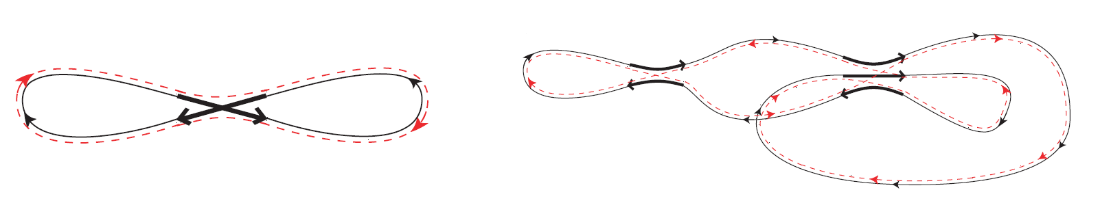
Figure 1: Pairs of orbits differing in encounters: Simplified sketch of a Sieber-Richter pair of orbits differing by their connections in a single encounter of two orbit parts, and a pair of orbits differing in two encounters involving two and three orbit parts. (Pictures from [17]©American Physical Society).

Contributions of higher order in $1/\epsilon$ arise from pairs of orbits differing noticeably only in so-called encounters [16, 17]. Inside these encounters two or more parts of the same orbit come close up to time reversal, and a partner orbit can then obtained by connecting the ends of these orbit parts differently and a subsequent adjustment to obtain a valid periodic orbit satisfying the equations of motion. For time-reversal invariant systems one also has to include the case where parts of an orbit are almost mutually time reversed. Two simplified sketches of such pairs of orbits are shown in Fig. 1.

The existence of such pairs of orbits requires hyperbolicity which follows from the existence of a spectral gap. In a hyperbolic system the possible directions at each point in phase space (apart from the direction of the flow and the direction of increasing energy) are spanned by pairs of stable and unstable directions. Deviations between (parts of) trajectories along the stable directions decrease exponentially in time, whereas deviations along stable directions increase exponentially but decrease for large negative times. This allows to ‘change connections’ inside an encounter, by constructing a part of an orbit $p^{\prime}$ that moves away from one part of $p$ and towards a different part of $p$; its deviation from the first part has to be unstable whereas the deviation from the second part is stable.

When deriving the contribution of such pairs of orbits for single-particle systems, the deviations between encountering parts of an orbit were measured in a system of coordinates associated to the stable and unstable directions [35, 36, 37]. This carries over in the present scenario as well. For example, if two parts come close we consider the points where these two parts pierce through a Poincaré surface of section in our reduced phase space. By transformation from the difference between the $I^{\prime}_{k}$, $\theta^{\prime}_{k}$ ($k=2,\ldots,L-1$) we then obtain $L-2$ pairs of coordinates $s_{k},u_{k}$ characterising the deviations between the two orbit parts in the stable and unstable directions. If the parts are almost time-reversed instead of close in phase space we instead have to consider the deviation of one part from the time-reversed of the other.

We can now determine the difference between the (reduced) actions of the partner orbits. Apart from the difference associated to the energy offset already seen in the diagonal approximation this has a further contribution accounting for the change of action due to the changed connections in the encounters. For an encounter of two parts the latter contribution can be written as [35, 36, 37]

$$\Delta S=\sum_{k}s_{k}u_{k}$$ (46)

where the sum runs over pairs of associated stable and unstable coordinates. Generalisations to encounters involving more orbit parts are given in [17]. As in the phase of (42) the action difference is divided by $\hbar$, systematic contributions of constructively interfering orbits will have action differences of this scale and hence very close encounters.

As a further ingredient one needs to determine the probability that encounters with given separations between the stretches arise in a periodic orbit/solution. For the corresponding formula we refer to [17]. We stress that the only requirement for its validity is the existence of spectral gap. This is used to derive an ‘ergodic’ probability for different parts of an orbit to come close, as well as an estimate for the duration of an encounter, both of which enter the formula.

With all ingredients for the single-particle treatment remaining valid, the contributions of all ‘diagrams’ of orbits differing in encounters (such as those displayed in Fig. 1) remain unchanged. These contributions involve powers of $1/\epsilon$ with the power increasing for more complex diagrams. The sum over all diagrams can be performed using the combinatorial techniques discussed in [17]. For systems without time-reversal invariance the contributions cancel leaving only the diagonal approximation. For time-reversal invariant systems one obtains a series expansion to all orders in $1/\epsilon$. In either case the results agree with the non-oscillatory terms with coefficients $c_{n}$ in the random matrix prediction

$$R(\epsilon)\sim{\rm 1+Re}\sum_{n=2}^{\infty}(c_{n}+d_{n}e^{2i\epsilon})\left(\frac{1}{\epsilon}\right)^{n}.$$ (47)

Here systems without time-reversal invariance (as described by the Gaussian Unitary Ensemble) have $c_{2}=-\frac{1}{2}$ and $d_{2}=\frac{1}{2}$ and all other coefficients vanish. For time-reversal invariant systems (as described by the Gaussian Orthogonal Ensemble) we have $c_{2}=-1$, $c_{n}=\frac{(n-3)!(n-1)}{2i^{n}}$ for $n\geq 3$, $d_{2}=d_{3}=0$ and $d_{n}=\frac{(n-3)!(n-3)}{2i^{n}}$ for $n\geq 4$. We note that the treatment summarised here assumes that our system (in the reduced phase space) has no further symmetries as these would lead to additional pairs of orbits with similar or identical actions, such as mutually reflected orbits in a system with reflection symmetry. The oscillatory terms and systems with discrete geometric symmetries will be discussed later.

As in case of normal ordering the trace formula is modified to include the Solari-Kochetov (SK) phase, we have to check that this does not affect the results arising in the present approach. To do so, we note that the contributions to the double sum only involve differences between phases associated to closeby partner orbits. Due to $\psi\propto\frac{1}{\sqrt{\hbar}}$ the SK phase itself is of an order independent of $\hbar$. As the SK phase is time-reversal invariant the phases of two partner orbits can only differ due to the slight changes inside encounters. However for the encounters relevant for spectral statistics the encounters become very close in the semiclassical limit, meaning that the difference between the SK phases becomes negligible.

3.4 Oscillatory contributions

The random-matrix prediction (47) for $R(\epsilon)$ also involves oscillatory contributions proportional to ${\rm Re}\frac{1}{(i\epsilon)^{n}}e^{2i\epsilon}$. To access these contributions a more careful semiclassical approximation is needed [38, 18]. In this approximation the level density is accessed from spectral determinants via

$$d(E)=\frac{1}{\pi}{\rm Im}\frac{\partial}{\partial\eta}\frac{\det(E-\hat{H})}{\det(E+\eta-\hat{H})}\big{|}_{\eta=0}.$$ (48)

An approximation for the spectral determinant on the level of the trace formula is

$$\det(E-\hat{H}) \propto \exp\left(-\int dE^{\prime}{\rm tr}(E^{\prime}-\hat{H})^{-1}\right)$$ (49)

$$\propto e^{-i\pi\bar{N}(E)}\sum_{\Gamma}F_{\Gamma}(-1)^{n_{\Gamma}}e^{iS_{\Gamma}(E)/\hbar}.$$

Here the sum is taken over sets of orbits $\Gamma$ with $n_{\Gamma}$ elements and cumulative reduced action $S_{\Gamma}$; the amplitude $F_{\Gamma}$ depends on the stability and the Maslov indices of the contributing orbits and $\bar{N}(E)$ is the smooth approximation for the number of energy levels below $E$. However using the spectral determinant allows to incorporate further quantum mechanical information, in particular the fact that due to $\hat{H}$ being Hermitian $\det(E-\hat{H})$ has to be real for real arguments $E$. As shown in [38] this leads to an approximation for the spectral determinant where the contributions from sets of orbits with cumulative periods larger than half of the Heisenberg tine $T_{H}=2\pi\hbar\bar{d}$ are replaced by the complex conjugate of the contributions from sets with cumulative periods below this threshold. This ‘Riemann-Siegel lookalike formula’ readily generalises to the many-body systems under consideration as its key ingredient, the semiclassical approximation for the trace of the resolvent $(E-{\hat{H}})^{-1}$, can be accessed from the trace of the propagator as above; essentially one only has to omit the restriction to the imaginary part in (13). Again periodicity is required only in the reduced phase space.

Using the improved approximation of the level density as well as the same general ideas as outlined above it is possible to resolve oscillatory contributions as well. As each level density brings in two determinants, evaluating the two-point correlation function then requires to study interference between quadruplets of (possibly empty) sets of orbits. Hence one also needs to take into account contributions where, say, after changing connections inside encounters an orbit is broken into two orbits with similar cumulative action. A treatment of these more involved correlations shows that for chaotic quantum systems $R(\epsilon)$ fully agrees with the predictions from RMT [18].

3.5 Systems without a spectral gap

Interestingly, there are chaotic systems that do not have a spectral gap but still satisfy some of the ingredients of our calculation, such as hyperbolicity which is required for the existence of orbit pairs differing in encounters. For these systems many of the techniques sketched here are applicable, but the final result of Wigner-Dyson statistics does not carry over as e.g. the sum rule (44) becomes invalid. An interesting question for future work is whether chaotic many-body systems without a spectral gap could be faithful to RMT ensembles that incorporate more information about the problem at hand and reduce to Wigner-Dyson statistics in important regimes, e.g. the embedded many-body ensembles [39, 40] or ensembles sensitive to the spacial structure of the problem. An example for a situation where the spacial structure is important is the continuum limit with diverging number of sites; additional orbit correlations relevant in this case were identified in [41].

4 Symmetries

In a system with additional discrete symmetries one needs to consider the spectral statistics inside subspectra determined by the symmetry group. A prime example is the discrete (disorder-free) Bose-Hubbard model with periodic boundary conditions as introduced above. Its symmetry group is the dihedral group, consisting of the discrete translation $\psi_{k}\to\psi_{k+1}$ and its iterates; the reflection $\psi_{k}\to\psi_{L-1-k}$; and combinations of translations and reflection that can be viewed here as reflection about a different centre. More formally the symmetry group for this model is the dihedral group $D_{L}$. Here $D_{n}$ stands for the dihedral group of order $2n$. The spectrum of the Bose-Hubbard model decomposes into subspectra labelled by the eigenvalues $e^{2\pi i\kappa/L}$ of the discrete translation operator where $\kappa=0,\dots,L-1$ denotes the quasi-momentum. The spectra with $\kappa=0$ and (if integer) $\kappa=L/2$ decompose further into components even and odd under reflection, whereas the remaining subspectra come in energy-degenerate pairs $\kappa$, $L-\kappa$ related by reflection. Altogether we obtain $L+1$ subspectra for odd $L$ and $L+2$ subspectra for even $L$. A representation-theoretic justification of this decomposition will be given below and we refer to [42] for ways to implement the decomposition numerically.

The level density associated to each subspectrum is obtained using a trace formula where the classical orbits, or in the present context the solutions of the Gross-Pitaevski equation, are required to be periodic (in the sense above) inside a fundamental domain of the system [43]. (See also [44].) For the case at hand this domain can be defined e.g. by converting $\psi_{k}^{\prime}$ to $\psi_{k}$ for a fixed choice of $\psi_{0}^{\prime}$ and then imposing certain conditions on $\psi_{k}$. Demanding that ${\rm Re}\psi_{k}$ is smallest for $k=0$ guarantees that applying the translation operator to a point inside the fundamental domain leads to a point outside. The same applies to most other elements of the symmetry group but in order to guarantee that reflection about the 0-th site leads outside the fundamental domain we need an additional requirement such as ${\rm Re}\psi_{1}<{\rm Re}\psi_{L-1}$.

Each subspectrum $\alpha$ (not distinguishing between degenerate subspectra) can now be associated to an irreducible representation of the symmetry group, and the corresponding trace formula [43] has a form similar to (1),

$$d_{\alpha}(E)\approx\bar{d}_{\alpha}(E)+\frac{1}{\pi\hbar}{\rm Re}\sum_{p}\chi_{\alpha}(g_{p})A_{p}e^{iS_{p}/\hbar}\ .$$ (50)

The only difference from (1) apart from the restriction to the fundamental domain is the additional factor $\chi_{\alpha}(g_{p})$. Here $g_{p}$ is the group element relating the initial and final point of the orbit $p$ if the orbit is considered in the full phase space as opposed to the fundamental domain. The character $\chi_{\alpha}(g_{p})$ is the trace of the matrix representing $g_{p}$ in the representation $\alpha$. As in [43] the derivation of (50) requires that a projection operator on the part of the Hilbert space associated to our subspectrum is inserted inside the trace taken over the Hilbert space; doing this in our many-particle calculations starting from (13) leads to exactly the same modifications as observed in [43] for single-particle systems.

To apply (50) to the Bose-Hubbard model we need the irreducible representations of the dihedral group [45]. The representation of the translation operator must have an $L$-fold power $\mathbb{I}$; its two-dimensional representations are therefore be given by

$$\begin{pmatrix}\cos\frac{2\pi\kappa}{L}&-\sin\frac{2\pi\kappa}{L}\\ \sin\frac{2\pi\kappa}{L}&\cos\frac{2\pi\kappa}{L}\\ \end{pmatrix}.$$ (51)

The reflection operator is then represented by

$$\begin{pmatrix}1&0\\ 0&-1\\ \end{pmatrix}$$ (52)

and the representations of all other group elements can be found using that the matrix representation of a product of symmetry operations must be the product of the matrix representations. The general theory of symmetries in quantum mechanics (see e.g. [46]) implies that the energy eigenstates associated to this representation can be grouped into pairs (representable as vectors) with identical energy. One can show that for the two-dimensional representation at hand this leads precisely to the energy-degenerate subspectra associated to eigenvalues of the translation operator $e^{2\pi i\kappa/L}$ ($\kappa\neq 0,\frac{L}{2}$) as mentioned above.

However if we have $\kappa=0$ or, assuming even $L$, $\kappa=\frac{L}{2}$ the matrix (51) becomes diagonal and the two-dimensional representations defined above become reducible. Instead of using these representations the associated subspectra therefore have to be described by one-dimensional representations. These represent the translation operator either by 1 or in case of even $L$ alternatively by -1, whereas the reflection operator can be represented by either $1$ or $-1$ regardless of $L$. Again these spectra precisely correspond to what we said above about the cases $\kappa=0,\frac{L}{2}$.

In general the consideration of discrete symmetries can change the appropriate RMT ensemble compared to the one expected based on the time-reversal properties alone [47]. However using Eq. (50) one can show that this does not happen for subspectra associated to representations by real matrices [48, 49]. As the aforementioned representations of the dihedral group are real the spectral statistics of all its subspectra is thus in line with the GOE as observed numerically in [22] as well as in the next section.

5 Numerical results

To support our results numerically and complement the previous numerical studies we have performed a numerical analysis of the chaotic properties of both the quantum and the classical Bose-Hubbard model. Our results support Wigner-Dyson statistics as well as mostly classical chaotic dynamics in the regime where the hopping and interaction terms are comparable.

For the quantum model we are interested in the spectral statistics as discussed above. We use a statistical observable slightly more convenient for computations than $R(\epsilon)$, namely the normalised distribution $P(r)$ of ratios between subsequent level spacings; if the ordered quantum levels are denoted by $E_{n}$, these ratios are given by $r_{n}=\dfrac{E_{n+1}-E_{n}}{E_{n}-E_{n-1}}$. The ratio distribution is especially suited for our purposes as there is no requirement to explicitly evaluate the average level density. A random matrix prediction for $P(r)$ was obtained in [50] by considering $3\times 3$ random matrices; for the GOE it reads

$$P_{RMT}(r)=\dfrac{27}{8}\dfrac{r+r^{2}}{(1+r+r^{2})^{5/2}}\ .$$ (53)

In particular for $r\to 0$ one can see that $P(r)\propto r$, which is due to level repulsion. Notice that for large $r$ the distribution has a fat tail in contrast to the level spacing distribution: $P(r)\propto r^{-3}$ for $r\gg 1$. As for the density of nearest-neighbour spacings the results for large matrices are expected to be very similar in value but analytically more complicated. For comparison, we mention that the ratio distribution for an integrable system (assuming that the energy levels are independent) is given by

$$P_{Poisson}(r)=\dfrac{1}{(1+r)^{2}}\ .$$ (54)

We determined the spectrum of the quantum Bose-Hubbard model via exact diagonalisation. For each of the subspectra described in section 4 we computed the histogram of $r$ to get a numerical estimate of the ratio distribution $P_{\rm num}(r)$. Examples of such numerical histograms are displayed in Fig. 2.

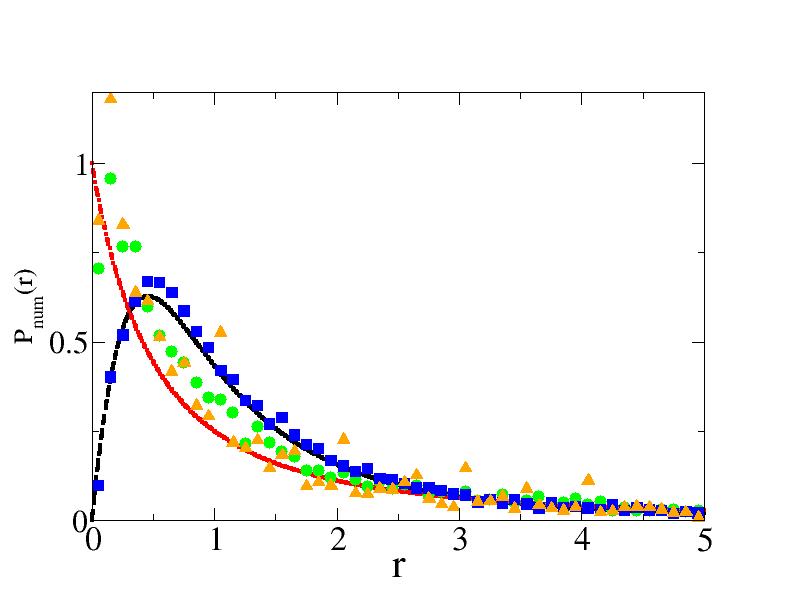
Figure 2: Numerical estimate of the ratio distribution between neighbouring levels for the quantum Bose Hubbard model with $L=5$ and $N=25$. The dashed black line stands for the RMT prediction (53). The dotted-dashed red line stands for the Poisson distribution (54). Green circles: $UN/J=0.125$. Blue squares: $UN/J=5$. Orange triangles: $UN/J=250$.

Then we determined the $L^{1}$ norm (i.e. the integral over the absolute value) of the difference $P_{\rm num}(r)-P_{RMT}(r)$. Finally this difference was averaged over all different subspectra. Fig. 3 top shows the norm for the case $L=5$ and $N=15$ as well as $N=25.$ We obtain good agreement for the case that the interaction term (of order $UN^{2}$) is comparable to or slightly larger than the hopping term (of order $JN$). The agreement improves as $N$ increases, which is reassuring as our theoretical derivation of Wigner-Dyson statistics holds in the limit $N\to\infty$ (or equivalently in the semiclassical limit).

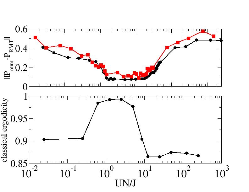
Figure 3: Top: Comparison between the ratio distribution of neighbouring levels between the Bose-Hubbard model and RMT for $N=25$ (black circles) and $N=15$ (red squares), and $L=5$. The difference is estimated via the L¹ norm of the deviation from RMT as a function of $UN/J$. Bottom: Numerical estimate of the degree of ergodicity of the classical dynamics of Bose-Hubbard model with $N=25$ and $L=5$ as a function of $UN/J$. $1$ indicates full ergodicity. The precise definition of our estimate is given in the text.

For the classical Bose-Hubbard model we introduce a numerically determined measure of ergodicity, which indicates whether the classical limit is mostly chaotic. To determine this measure we considered the Hamiltonian

$$H(\boldsymbol{\psi}^{*},\boldsymbol{\psi})=-\frac{J}{2}\sum_{k=0}^{L-1}(\psi^{*}_{k+1}\psi_{k}+\psi^{*}_{k}\psi_{k+1})+\frac{U}{2}\sum_{k=0}^{L-1}(\psi_{k}^{*})^{2}\psi_{k}^{2}$$ (55)

where we identified $\psi_{L}=\psi_{0}$ and $\psi_{L}^{*}=\psi_{0}^{*}$. The classical dynamics is given by

$$i\hbar\dot{\boldsymbol{\psi}}=\frac{\partial H}{\partial\boldsymbol{\psi}^{*}},\quad i\hbar\dot{\boldsymbol{\psi}}^{*}=-\frac{\partial H}{\partial\boldsymbol{\psi}}.$$ (56)

If an initial point $(\boldsymbol{\psi}^{*}_{0},\boldsymbol{\psi}_{0})$ is given in phase space, Eq. (56) allows to compute the unique trajectory $(\boldsymbol{\psi}^{*}(t),\boldsymbol{\psi}(t))$ such that $(\boldsymbol{\psi}^{*}(0),\boldsymbol{\psi}(0))=(\boldsymbol{\psi}^{*}_{0},\boldsymbol{\psi}_{0})$. It may be useful to add that as each point is part of a classical trajectory the point $(\boldsymbol{\psi}^{*}_{0},\boldsymbol{\psi}_{0})$ is parameterised by $2L$ real numbers as the coefficients of $\boldsymbol{\psi}^{*}_{0}$ are the complex conjugates of the coefficients of $\boldsymbol{\psi}_{0}$.

As the energy $E$ and the particle number $N$ are conserved, the trajectory can only access a subspace in phase space, denoted by ${\cal M}_{N,E}$, which is the constant energy surface associated to $E$ in the Fock space with $N$ particles. Numerically a triangulation of ${\cal M}_{N,E}$ is performed by picking random points on this surface. These points are generated using Halton sequences, which are commonly used to explore high dimensional spaces. First a random point is sampled on the hypersphere $||\boldsymbol{\psi}||^{2}=N$. If its energy coincides with $E$ it is kept and stored as a point in ${\cal M}_{N,E}$. Otherwise we continue the sampling. In order to cover substantially ${\cal M}_{N,E}$ for typical values of $E$, $UN/J$ we chose to pick $2\times 10^{6}$ random points. Then the mean distance between any two of these points is calculated, let us call it $\delta$. This gives a typical distance scale for the constant energy surface at a given energy $E$. This typical distance is used to define balls of radius $\delta/10$ around each points. After having determined a cover of ${\cal M}_{N,E}$ the trajectory starting from $(\boldsymbol{\psi}^{*}_{0},\boldsymbol{\psi}_{0})$ is computed for a sequence of increasing (final) times. We took large enough final values of the propagation time so that the number of visited balls does not vary significantly after this time.

Finally a measure for the ergodicity of a trajectory is defined by the ratio between the number of visited balls and the total number of balls. In order to have generic values, this ergodicity measure is averaged over different choices of initial conditions $(\boldsymbol{\psi}^{*}_{0},\boldsymbol{\psi}_{0})$. Our results are displayed in Fig. 3 bottom. By definition our measure is a real number between $0$ and $1$. $1$ indicates perfect ergodicity. The closer it is to $1$ the more ergodic the trajectory is. While not a rigorous check of the conditions for random matrix statistics, our measure indicates whether the system is mostly ergodic or has a substantially mixed phase space with large stability islands. Fig. 3 bottom shows that, for the same range of $UN/J$, the classical dynamics is predominantly ergodic and the quantum system agrees closely with RMT prediction.

Our results are compatible with those obtained through a different approach and a modified version of the model in [51]. There the authors chose a different normalisation of $\boldsymbol{\psi}$ and claimed that their version of the classical Bose-Hubbard model becomes more and more classical when increasing $U/J$. This is line with the left part of Fig. 3 bottom.

Appendix A Perturbation of the stability matrix and the Hessian

In this appendix we want to explicitly show how perturbation theory can be used to deal with the vanishing eigenvalues of the stability matrix and the Hessian considered in subsection 2.5, associated to $k=0$ and $k=1$. To avoid some of the complexity of [25] we specifically consider small perturbations $\delta H$ that depend only on $\theta^{\prime}_{k}$, which does not appear as a parameter of the unperturbed Hamiltonian. In order to avoid ambiguities we choose $\delta H(\theta^{\prime}_{k})$ periodic in $\theta^{\prime}_{k}$ with the period coinciding with the range of values covered by $\theta^{\prime}_{k}$.

We first investigate how the perturbation modifies the vanishing eigenvalue of the Hessian ${\cal H}$. The corresponding eigenvector is associated to a simultaneous shift of $\theta^{\prime}_{jk}$ for our $k$ at all time steps $j$. It is thus convenient to rewrite the Hessian in terms of derivatives w.r.t. $I^{\prime}_{jk}$, $\theta^{\prime}_{jk}$ ; this also absorbs the divisor $\hbar$ in (2.4) and it has the advantage that the Hessian becomes Hermitian. The perturbation of the Hessian $\delta{\cal H}$ has as its only non-vanishing matrix elements the derivatives $-\frac{\partial^{2}\delta H(\theta^{\prime}_{jk})}{\partial{\theta^{\prime}}_{jk}^{2}}\tau$. In the same coordinate system the eigenvector $\boldsymbol{e}$ associated to the vanishing eigenvalue has identical entries for the ${\cal J}$ components associated to the $\theta^{\prime}_{jk}$ associated to our $k$ and the remaining components are zero. First-order perturbation theory then yields a perturbed eigenvalue

$$\frac{\boldsymbol{e}\cdot\delta{\cal H}\boldsymbol{e}}{\boldsymbol{e}\cdot\boldsymbol{e}}=-\frac{1}{{\cal J}}\sum_{j}\frac{\partial^{2}\delta H(\theta^{\prime}_{jk})}{\partial{\theta^{\prime}}_{jk}^{2}}\tau$$ (57)

taken as $\epsilon$ in subsection 2.5.

To study the effect on the stability matrix we first consider the matrix $\tilde{M}_{j}^{(k)}$ mapping a deviation of $(\theta^{\prime}_{jk},I^{\prime}_{jk})$ to the resulting deviation after a time step of size $\tau$. We obtain, e.g. by converting Eq. (27) to the present system of coordinates,

$$\tilde{M}_{j}^{(k)}=\begin{pmatrix}1+\frac{\partial^{2}H(\boldsymbol{\theta}_{j},\boldsymbol{I}_{j})}{\partial I^{\prime}_{jk}\partial\theta^{\prime}_{jk}}\tau&\frac{\partial^{2}H(\boldsymbol{\theta}_{j},\boldsymbol{I}_{j})}{\partial{I^{\prime}}_{jk}^{2}}\tau\\ -\frac{\partial^{2}H(\boldsymbol{\theta}_{j},\boldsymbol{I}_{j})}{\partial{\theta^{\prime}}_{jk}^{2}}\tau&1-\frac{\partial^{2}H(\boldsymbol{\theta}_{j},\boldsymbol{I}_{j})}{\partial\theta^{\prime}_{jk}\partial{I^{\prime}}_{jk}}\tau\end{pmatrix}.$$ (58)

Here the lower left entry vanishes for the unperturbed Hamiltonian but is moved away from zero by the perturbation $\delta H(\theta^{\prime}_{k})$. As a consequence of this perturbation the product given in (32)

$$\tilde{M}^{(k)}=\begin{pmatrix}1&\frac{d\Delta\theta_{k}^{\prime}}{dI^{\prime}_{k}}\\ 0&1\end{pmatrix}$$ (59)

then receives the lower left entry

$$-\sum_{j}\frac{\partial^{2}\delta H(\theta_{jk}^{\prime})}{\partial{\theta^{\prime}}_{jk}^{2}}\tau=\epsilon{\cal J}$$ (60)

as desired. In contrast the changes of the other entries do not affect the determinant to linear order in the perturbation.

Appendix B Weyl ordering

Finally we want to show explicitly that in line with [27, 24, 25, 9, 33] the SK phase does not arise in case of Weyl ordering. Using the Hamiltonian in Weyl ordering the short-time propagator can be written as [33]

$$\left\langle\boldsymbol{\psi}_{j}|e^{-\frac{i}{\hbar}\hat{H}\tau}|\boldsymbol{\psi}_{j-1}\right\rangle\approx 2^{L}\int d[\boldsymbol{w}_{j},\boldsymbol{w}_{j}^{*}]\exp\Big{(}-2|\boldsymbol{w}_{j}|^{2}+2\boldsymbol{\psi}_{j}^{*}\cdot\boldsymbol{w}_{j}+2\boldsymbol{\psi}_{j-1}\cdot\boldsymbol{w}_{j}^{*}$$

$$-|\boldsymbol{\psi}_{j}|^{2}/2-|\boldsymbol{\psi}_{j-1}|^{2}/2-\boldsymbol{\psi}_{j}^{*}\cdot\boldsymbol{\psi}_{j-1}-\frac{i}{\hbar}H(\boldsymbol{w}_{j}^{*},\boldsymbol{w}_{j})\tau\Big{)}$$ (61)

involving an integration over a pair of complex conjugate variables $\boldsymbol{w}_{j},\boldsymbol{w}_{j}^{*}$ that were not required in normal ordering. The action in the discretised coherent-state path integral then turns into [33]

$$R = \sum_{j}\Big{(}\frac{\hbar}{i}(-2|\boldsymbol{w}_{j}|^{2}+2\boldsymbol{\psi}_{j}^{*}\cdot\boldsymbol{w}_{j}+2\boldsymbol{\psi}_{j-1}\cdot\boldsymbol{w}_{j}^{*}-|\boldsymbol{\psi}_{j}|^{2}/2-|\boldsymbol{\psi}_{j-1}|^{2}/2$$ (62)

$$-\boldsymbol{\psi}_{j}^{*}\cdot\boldsymbol{\psi}_{j-1})-H(\boldsymbol{w}_{j}^{*},\boldsymbol{w}_{j})\tau\Big{)}$$

and the path integral runs over $\boldsymbol{w}_{j},\boldsymbol{w}_{j}^{*}$ as well as $\boldsymbol{\psi}_{j},\boldsymbol{\psi}_{j}^{*}$. The action becomes stationary under variation of $\boldsymbol{\psi}_{j},\boldsymbol{\psi}_{j}^{*}$ if

$$\boldsymbol{w}_{j}=\frac{\boldsymbol{\psi}_{j}+\boldsymbol{\psi}_{j-1}}{2}$$ (63)

and its complex conjugate hold. This suggests that in the limit of fine discretisation the $\boldsymbol{w}_{j}$ should be interpreted as macroscopic wave functions halfway between two discretisation steps. Furthermore stationarity w.r.t. variation of $\boldsymbol{w}_{j},\boldsymbol{w}_{j}^{*}$ implies

$$i\hbar\frac{\boldsymbol{w}_{j}-\boldsymbol{\psi}_{j-1}}{\tau/2}=\frac{\partial H(\boldsymbol{w}_{j}^{*},\boldsymbol{w}_{j})}{\partial\boldsymbol{w}_{j}^{*}}$$ (64)

and its complex conjugate, which is the appropriate discretisation of the nonlinear Schrödinger equation $i\hbar\dot{\boldsymbol{\psi}}=\frac{\partial H}{\partial\boldsymbol{\psi}^{*}}$ for the time interval $\tau/2$. After eliminating $\boldsymbol{w}_{j}$ with the help of (63) a short calculation shows that the combination of macroscopic wave functions in the action (62) agrees with the simpler form in (12).

We now have to evaluate the Hessian of $\frac{R}{\hbar}$ and its determinant. In analogy to subsection 2.4 we start with the Hessian containing all second derivatives. If we first write the derivatives w.r.t. all $\boldsymbol{w}_{j}^{*},\boldsymbol{w}_{j}$ and then those w.r.t. all $\boldsymbol{\psi}_{j}^{*},\boldsymbol{\psi}_{j}$ the Hessian assumes the form $i\begin{pmatrix}D&-2E\\ -2E^{T}&E+E^{T}\\ \end{pmatrix}$ where $D$ is block-diagonal with the blocks

$$D_{j}=2\mathbb{I}_{2L}+\frac{i\tau}{\hbar}\frac{\partial^{2}H(\boldsymbol{w}_{j}^{*},\boldsymbol{w}_{j})}{\partial(\boldsymbol{w}_{j}^{*},\boldsymbol{w}_{j})^{2}}$$ (65)

and the orthogonal matrix $E$ is given by

$$E=\begin{pmatrix}0&\mathbb{I}_{L}&&\\ &\ddots&\ddots&\\ &&\ddots&\mathbb{I}_{L}\ \\ \mathbb{I}_{L}\ &&&0\\ \end{pmatrix}.$$ (66)

The determinant can now be evaluated as

$$\det i\begin{pmatrix}D&-2E\\ -2E^{T}&E+E^{T}\\ \end{pmatrix}$$

$$= \det(2E^{T})\det(2E-D(2E^{T})^{-1}(-E-E^{T}))$$

$$= \det(D+DE^{2}-4E)$$

$$= \det\begin{pmatrix}D_{0}+4F&D_{0}+4F^{T}&&&\\ &D_{1}+4F&D_{1}+4F^{T}&&\\ &&\ddots&\ddots&\\ D_{{\cal J}-1}+4F^{T}&&&&D_{{\cal J}-1}+4F\end{pmatrix}$$

with $F=\begin{pmatrix}0&\mathbb{I}_{L}\\ 0&0\end{pmatrix}$. Here the factor $i$ dropped out because the dimension of the matrix is a multiple of 4. As the final matrix is of block tridiagonal form it can be simplified with the help of (24). Using

$$\det(D_{j}+4F^{T}) = 4^{L}+O(\tau^{2})$$

$$(D_{j}+4F^{T})^{-1}(D_{j}+4F) = \tilde{M}_{j}+O(\tau^{2})$$

(where $\tilde{M}_{j}$ is defined as in (27) but with $\boldsymbol{w}_{j},\boldsymbol{w}_{j}^{*}$ taking the role of $\boldsymbol{\psi}_{j},\boldsymbol{\psi}_{j}^{*}$) and again ignoring terms of quadratic and higher order in $\tau$ in the entries we obtain

$$\det\begin{pmatrix}D&2E\\ 2E^{T}&-E-E^{T}\end{pmatrix}=4^{{\cal J}L}\det(\tilde{M}-\mathbb{I}_{2L}).$$ (67)

As usual the stationary-phase approximation requires the inverse square root of this determinant, containing a factor $2^{-{\cal J}L}$. This factor is cancelled by the $2^{{\cal J}L}$ in the integration measure for $\boldsymbol{w}_{j},\boldsymbol{w}_{j}^{*}$. As anticipated, we thus obtain the same result as with normal ordering apart from the SK phase. The remaining steps, in particular taking into account the conservation laws, carry over directly from the case of normal ordering discussed in the main text.

References

References

- [1] Schulman L S 1981 Techniques and Applications of Path Integration (Wiley Interscience Public.)
- [2] van Vleck J H 1926 Bull. Natl. Res. Council 10 1
- [3] Gutzwiller M 1971 J. Math. Phys. 12 343
- [4] Haake F 2010 Quantum Signatures of Chaos 3rd ed (Springer)
- [5] Stöckmann H-J 1999 Quantum Chaos: An Introduction (Cambridge University Press)
- [6] Gutzwiller M 1990 Chaos in Classical and Quantum Mechanics (Springer)
- [7] Negele J W 1982 Rev. Mod. Phys. 54 913
- [8] Braun C Garg A 2011 J. Math. Phys. 48, 032104
- [9] Viscondi T F and de Aguiar M A M 2011 J. Math. Phys. 52 052104
- [10] Engl T, Dujardin J, Argüelles A, Schlagheck P, Richter K, and Urbina J 2014 Phys. Rev. Lett. 112 140403
- [11] Engl T, Plößl P, Urbina J, and Richter K 2014, Theoretical Chemistry Accounts 133 1563; Engl T, Urbina J, and Richter K 2014 arXiv:1409.5684 [cond-mat.mes-hall]
- [12] Bohigas O, Giannoni M J, and Schmit C 1984 Phys. Rev. Lett. 52 1; Casati G, Valz-Gris F, and Guarneri I 1980 Lett. Nuovo Cim. 28 279 (1980); Berry M V 1981, Ann. Phys. (N.Y.) 131 163
- [13] Berry M V 1985 Proc. R. Soc. Lond. Ser. A 400 229
- [14] Hannay J H and Ozorio de Almeida A M 1984 J. Phys. A 17 3429
- [15] Argaman N, Dittes F M, Doron E, Keating J P, Kitaev A Yu, Sieber M, and Smilansky U 1993 Phys. Rev. Lett. 71 4326
- [16] Sieber M and Richter K 2001 Physica Scripta T90 128; M. Sieber 2002 J. Phys. A 35 L613
- [17] Müller S, Heusler S, Braun P, Haake F, and Altland A 2004 Phys. Rev. Lett. 93, 014103; Müller S, Heusler S, Braun P, Haake F, and Altland A 2005 Phys. Rev. E 72, 046207.
- [18] Heusler S, Müller S, Altland A, Braun P, and Haake F 2007 Phys. Rev. Lett. 98 044103; Keating J P and Müller S 2007 Proc. R. Soc. Lond. A 463 3241; Müller S, Heusler S, Altland A, Braun P, and Haake F 2009 New J. Phys. 11 103025
- [19] Balian R and Bloch C 1970 Ann. Phys. 60 401; ibid. 1971 Ann. Phys. 64 271; ibid. 1972 Ann. Phys. 69 76
- [20] Kolovsky A R 2007 Phys. Rev. Lett. 99 020401
- [21] Kolovsky A R and Buchleitner A 2004 Europhys. Lett. 68 632
- [22] Kollath C, Roux G, Biroli G, and Läuchli A M 2010 J. Stat. Mech. P08011
- [23] Montambaux G, Poilblanc D, Bélissard J, Sire C 1993 Phys. Rev. Lett. 70 497; Jacquod P, Shepelyansky D L 1997 Phys. Rev. Lett. 79 1837; Georgeot B, Shepelyansky D L 1997 Phys. Rev. Lett. 79 4365; Georgeot B, Shepelyansky D L 1998 Phys. Rev. Lett. 81 5129
- [24] Mehlig B and Wilkinson M 2001 Ann. Phys. (Lpz) 10 541
- [25] Muratore-Ginanneschi P 2003 Phys. Rep. 383 299
- [26] Altland A and Simons B 2010 Condensed Matter Field Theory 2nd ed (Cambridge University Press)
- [27] Baranger M, Aguiar M A M, Keck F, Korsch H-J, and Schellhaaß B 2001 J. Phys. A 34 7227
- [28] Creagh S C and Littlejohn R G 1991 Phys. Rev. A 44 836
- [29] Molinari L G 2008 Linear Algebra Appl. 429 2221
- [30] Solari H G 1987 J. Math. Phys. 28 1097
- [31] Kochetov E A 1995 J. Math. Phys. 36 4667
- [32] Hummel Q, Urbina J and Richter K 2014 J. Phys. A: Math. Theor. 47 015101
- [33] dos Santos L C and de Aguiar M A M 2006 J. Phys. A: Math. Gen. 39 13465
- [34] Müller S and Sieber M 2011 Quantum Chaos and Quantum Graphs The Oxford Handbook of Random Matrix Theory ed G Akemann (Oxford: Oxford University Press)
- [35] Turek M and Richter K 2003 J. Phys. A: Math. Gen. 36 L455
- [36] Spehner D 2003 J. Phys. A: Math. Gen. 36 7269
- [37] Turek M, Spehner D, Müller S, and Richter K 2005 Phys. Rev. E 71 016210
- [38] Berry M V and Keating J P 1990 J. Phys. A: Math. Gen. 23 4839; Keating J P 1992 Proc. R. Soc. Lond. A 436 99; Berry M V and Keating J P 1992 Proc. R. Soc. Lond. A 437 151
- [39] Mon K K and French J B 1975 Ann. Phys. (N.Y.) 95 90
- [40] Benet L and Weidenmüller H A 2003 J. Phys. A: Math. Gen. 36 3569
- [41] Gutkin B and Osipov V 2015 Nonlinearity 29 325
- [42] Sandvik A W 2010 AIP Conf. Proc. 1297 135
- [43] Robbins J M 1989 Phys. Rev. A 40 2128
- [44] Seligman T H and Weidenmüller H A 1994 J. Phys. A: Math. Gen. 27 7915
- [45] Kosmann-Schwarzbach Y 2000 Groups and Symmetries (Springer)
- [46] Elliot J P and Dawber P G 1979 Symmetry in Physics (Macmillan)
- [47] Leyvraz F, Schmit C and Seligman T 1996 J. Phys. A: Math. Gen. 29 L575
- [48] Keating J P and Robbins J M 1997 J. Phys. A: Math. Gen. 30 L177
- [49] Joyner C H, Müller S, and Sieber M 2012 J. Phys. A: Math. Theor. 45 205102
- [50] Atas Y Y, Bogomolny E, Giraud O, and Roux G 2013 Phys. Rev. Lett. 110 084101
- [51] Cassidy A C, Mason D, Dunjko V, Olshanii M 2009 Phys. Rev. Lett. 102 025302