Index statistical properties of sparse random graphs

Abstract

Using the replica method, we develop an analytical approach to compute the characteristic function for the probability $\mathcal{P}_{N}(K,\lambda)$ that a large $N\times N$ adjacency matrix of sparse random graphs has $K$ eigenvalues below a threshold $\lambda$. The method allows to determine, in principle, all moments of $\mathcal{P}_{N}(K,\lambda)$, from which the typical sample to sample fluctuations can be fully characterized. For random graph models with localized eigenvectors, we show that the index variance scales linearly with $N\gg 1$ for $|\lambda|>0$, with a model-dependent prefactor that can be exactly calculated. Explicit results are discussed for Erdös-Rényi and regular random graphs, both exhibiting a prefactor with a non-monotonic behavior as a function of $\lambda$. These results contrast with rotationally invariant random matrices, where the index variance scales only as $\ln N$, with an universal prefactor that is independent of $\lambda$. Numerical diagonalization results confirm the exactness of our approach and, in addition, strongly support the Gaussian nature of the index fluctuations.

I Introduction

Since the pioneering work of Wigner in the statistics of nuclear energy levels Wigner (1951), random matrix theory has established itself as a research field on its own, with many important applications in physics and beyond Mehta (2004). Valuable information on the behavior of different systems may be extracted from the eigenvalue statistics of related random matrix models. In this respect, meaningful statistical observables are the eigenvalue distribution, the distribution of extreme eigenvalues and the nearest-level spacing distribution, to name just a few Mehta (2004).

Another prominent observable is the index $\mathcal{K}_{N}(\lambda)$ of a $N\times N$ random matrix, defined here as the total number of eigenvalues below a threshold $\lambda$. The random variable $\mathcal{K}_{N}(\lambda)$ is of fundamental importance in the characterization of disordered systems described by a potential energy surface $\mathcal{H}(x_{1},\dots,x_{N})$ in the $N$-dimensional configurational space Wales (2003). The eigenvalues of the symmetric Hessian matrix $M$, formed by the second derivatives $M_{ij}=\partial^{2}\mathcal{H}/\partial x_{i}\partial x_{j}$, encode all information regarding the stability properties. The number of positive (negative) eigenvalues counts the number of stable (unstable) directions around a certain configuration, while the magnitude of an eigenvalue quantifies the surface curvature along the corresponding direction. In particular, the minima (maxima) of the potential energy are stationary points in which all Hessian eigenvalues are positive (negative). The index is a valuable tool to probe the energy landscape of systems as diverse as liquids Angelani et al. (2000); Broderix et al. (2000), spin-glasses Kurchan and Laloux (1996); Cavagna et al. (2000); Mehta et al. (2013), synchronization models Mehta et al. (2015) and biomolecules Wales (2003).

The simplest model for the Hessian of a disordered system consists in neglecting its dependency with respect to the configurations and assuming that the elements $M_{ij}$ are independently drawn from a Gaussian distribution. In this case, the Hessian belongs to the GOE ensemble of random matrices Mehta (2004) and the index statistics has been studied originally in reference Cavagna et al. (2000), using a fermionic version of the replica method. The authors have obtained the large-$N$ behavior of the index distribution $\mathcal{P}_{N}(K,\lambda)$

$$\mathcal{P}_{N}(K,\lambda)\sim\exp{\Bigg{\{}-\frac{\pi^{2}}{2\ln N}\left[K-Nm(\lambda)\right]^{2}\Bigg{\}}},$$ (1)

where $m(\lambda)=\int_{0}^{\lambda}d\lambda^{\prime}\rho(\lambda^{\prime})$ follows from the Wigner semi-circle law Mehta (2004) for the eigenvalue distribution $\rho(\lambda)$. Equation (1) implies that, for $N\gg 1$, the index variance scales logarithmically with $N$ and the typical fluctuations on a scale of width $O(\sqrt{\ln N})$ around the average index have a Gaussian form.

Recently, a significant amount of work has been devoted to study the index distribution of rotationally invariant ensembles, including Gaussian Majumdar et al. (2009, 2011), Wishart Majumdar and Vivo (2012) and Cauchy random matrices Marino et al. (2014). These models share the property that the joint probability distribution of eigenvalues is analytically known, which allows to employ the Coulomb gas technique, pioneered by Dyson Dyson (1962), to compute not only the typical index distribution, but also its large deviation regime, which characterizes atypical large fluctuations Majumdar et al. (2009, 2011); Majumdar and Vivo (2012); Marino et al. (2014). For all these ensembles, eq. (1) is recovered in the regime of small fluctuations, with a variance that grows as $\sigma^{2}\ln N$ for large $N$. The prefactor $\sigma^{2}$ is given by $\sigma^{2}=1/\pi^{2}$ for both Gaussian Cavagna et al. (2000); Majumdar et al. (2009, 2011) and Wishart Majumdar and Vivo (2012) random matrices, independently of $\lambda$, while $\sigma^{2}=2/\pi^{2}$ for Cauchy random matrices Marino et al. (2014). This logarithmic behavior of the variance apparently reflects the repulsion between neighboring levels Stöckmann (2006), which imposes a constraint on the total number of eigenvalues that fit in a finite region of the spectrum.

Despite the success of the Coulomb gas approach, the analytical form of the joint probability distribution of eigenvalues is not known for various interesting random matrix models. Perhaps the most representative example in this sense is the adjacency matrix of sparse random graphs Bollobás (1985); Wormald (1999), in which the average total number of nonzero entries scales only linearly with $N$. Although the eigenvalue distribution of random graphs has been computed using different techniques Rogers (2010), the statistical properties of the index have not been addressed so far. Several random graph models typically contain localized eigenvectors at finite sectors of the spectrum Fyodorov and Mirlin (1991); Biroli and Monasson (1999); Metz et al. (2010); Slanina (2012), usually corresponding to extreme eigenvalues, where the nearest-level spacing distribution follows a Poisson law Slanina (2012); Méndez-Bermúdez et al. (2015). In these regions, neighboring eigenvalues are free to be arbitrarily close to each other, which should heavily influence the index fluctuations. Models in which the state variables are placed on the nodes of random graphs have found an enormous number of applications, including spin-glasses, satisfiability problems, error-correcting codes and complex networks (see Mezard and Montanari (2009); Barrat et al. (2008) and references therein), and alternative tools to study their index fluctuations would be more than welcome.

In this paper we derive an analytical expression for the characteristic function of the index distribution describing the adjacency matrix of a broad class of random graphs, defined in terms of an arbitrary degree distribution. In principle, such analytical result allows to calculate the leading contribution in the large-$N$ limit of all moments of $\mathcal{P}_{N}(K,\lambda)$, yet we concentrate here on the first and second moments. Specifically, we show that the index variance of random graphs scales generally as $\sigma^{2}(\lambda)N$, with a prefactor $\sigma^{2}(\lambda)$ that depends on the threshold $\lambda$ and on the particular structure of the random graph model at hand. For random regular graphs with uniform edges, in which all eigenvectors are delocalized Jakobson et al. (1999); Oren and Smilansky (2010); Geisinger (2013), we show that $\sigma^{2}(\lambda)=0$ for any $\lambda$. On the other hand, for random graph models with localized eigenvectors Kühn (2008); Metz et al. (2010); Slanina (2012); Méndez-Bermúdez et al. (2015); Bapst and Semerjian (2011), the prefactor $\sigma^{2}(\lambda)$ exhibits a maximum for a certain $\lambda$, while it vanishes for $|\lambda|\rightarrow 0$. These results indicate that the linear scaling of the variance is a consequence of the uncorrelated nature of the eigenvalues in the localized regions of the spectrum. Since $\sigma^{2}(0)=0$ for random graphs with an arbitrary degree distribution, the linear scaling breaks down for $\lambda=0$ and the logarithmic scaling reemerges as the large-$N$ leading contribution for the index variance, which is supported by numerical diagonalization results. The model-dependent character of $\sigma^{2}(\lambda)$ contrasts with the highly universal prefactor found in rotationally invariant ensembles, though the typical index fluctuations of random graphs remain Gaussian distributed, as supported by numerical diagonalization results.

In the next section, we lay the ground for the replica computation of the characteristic function. The random graph model is introduced in section III, the replica approach is developed in section IV and the final analytical result for the characteristic function is presented in section V. We discuss explicit results for the average and the variance of the index in section VI and, in the final section, some final remarks are presented.

II The general setting

In this section we show how to recast the problem of computing the index distribution of a random matrix in terms of a calculation reminiscent from the statistical mechanics of disordered systems. Let us consider a $N\times N$ real symmetric matrix $A$ with eigenvalues $\lambda_{1},\dots,\lambda_{N}$. The density of eigenvalues between $\lambda^{\prime}$ and $\lambda^{\prime}+d\lambda^{\prime}$ reads

$$\rho_{N}(\lambda^{\prime})=\sum_{\alpha=1}^{N}\delta(\lambda^{\prime}-\lambda_{\alpha})\,.$$ (2)

The index is defined here as the total number of eigenvalues smaller than a threshold $\lambda$

$$\mathcal{K}_{N}(\lambda)=\int_{-\infty}^{\lambda}d\lambda^{\prime}\rho_{N}(\lambda^{\prime})=\sum_{\alpha=1}^{N}\Theta(\lambda-\lambda_{\alpha}),$$ (3)

where $\Theta(\dots)$ is the Heavside step function. The object $\mathcal{K}_{N}(\lambda)$ is also regarded as the integrated density of states or the cumulative distribution function. At this point we introduce the generating function

$$\mathcal{Z}_{N}(z)=\left(\frac{-i}{2\pi}\right)^{\frac{N}{2}}\int d\mbox{\boldmath$\phi$}\exp{\left[\frac{i}{2}\mbox{\boldmath$\phi$}^{T}.\left(\mbox{\boldmath$A$}-\mbox{\boldmath$I$}z\right)\mbox{\boldmath$\phi$}\right]},$$ (4)

with $\mbox{\boldmath$\phi$}=(\phi_{1},\dots,\phi_{N})$ and $z=\lambda-i\epsilon$, where $\epsilon>0$ is a regularizer that ensures the convergence of the above Gaussian integral and $I$ denotes the identity matrix. The vector components $\phi_{1},\dots,\phi_{N}$ are real-valued. By using an identity that relates the Heavside function with the complex logarithm, eq. (3) can be written in terms of $\mathcal{Z}_{N}(z)$ as follows

$$\mathcal{K}_{N}(\lambda)=\frac{1}{\pi i}\lim_{\epsilon\rightarrow 0^{+}}\left[\ln\mathcal{Z}_{N}(z^{*})-\ln\mathcal{Z}_{N}(z)\right]\,.$$ (5)

Equation (5) holds for a single matrix $A$ with an arbitrary dimension $N$.

An ensemble of random matrices is defined by a large set of instances of $A$ drawn independently from a distribution $p(\mbox{\boldmath$A$})$. In this paper, we are interested in computing the averaged index distribution

$$\mathcal{P}_{N}(K,\lambda)=\left\langle\delta\left[K-\mathcal{K}_{N}(\lambda)\right]\right\rangle,$$ (6)

where $\langle\dots\rangle$ denotes the ensemble average with $p(\mbox{\boldmath$A$})$. Using an integral representation of the Dirac delta and substituting eq. (5) in eq. (6), we obtain

$$\mathcal{P}_{N}(K,\lambda)=\int\frac{d\mu}{2\pi}e^{-i\mu K}\mathcal{G}_{N}(\mu,\lambda)\,,$$ (7)

where the characteristic function

$$\mathcal{G}_{N}(\mu,\lambda)=\lim_{\epsilon\rightarrow 0^{+}}\left\langle\left[\mathcal{Z}_{N}(z)\right]^{-\frac{\mu}{\pi}}\left[\mathcal{Z}_{N}(z^{*})\right]^{\frac{\mu}{\pi}}\right\rangle$$ (8)

contains the whole information about the statistical properties of the index. The moments of the index distribution are determined from

$$\langle K^{n}\rangle=(-i)^{n}\frac{\partial^{n}\mathcal{G}_{N}(\mu,\lambda)}{\partial\mu^{n}}\Bigg{|}_{\mu=0},\quad n\in\mathbb{N}.$$ (9)

The aim here is to compute the leading contribution to $\mathcal{G}_{N}(\mu,\lambda)$ for $N\rightarrow\infty$. According to eq. (8), $\mathcal{G}_{N}(\mu,\lambda)$ is calculated from the ensemble average of a function that contains real powers of the generating function, which is an unfeasible computation. In order to proceed further, we invoke the main strategy of the replica method and rewrite eq. (8) as follows

$$\mathcal{G}_{N}(\mu,\lambda)=\lim_{\epsilon\rightarrow 0^{+}}\lim_{n_{\pm}\rightarrow\pm\frac{\mu}{\pi}}\left\langle\left[\mathcal{Z}_{N}(z)\right]^{n_{-}}\left[\mathcal{Z}_{N}(z^{*})\right]^{n_{+}}\right\rangle\,.$$ (10)

The idea is to treat initially $n_{-}$ and $n_{+}$ as integers, which allows to compute the ensemble average. Once this average is calculated and the limit $N\rightarrow\infty$ is taken, we make an analytical continuation of $n_{\pm}$ to the real values $\pm\frac{\mu}{\pi}$.

III Random graphs with an arbitrary degree distribution

We study the index distribution of $N\times N$ symmetric adjacency matrices with the following entries

$$A_{ij}=c_{ij}J_{ij},$$ (11)

where $c_{ij}=c_{ji}$ and $J_{ij}=J_{ji}$. The variables $c_{ij}\in\{0,1\}$ encode the topology of the underlying random graph: we set $c_{ij}=1$ if there is an edge between nodes $i$ and $j$, and zero otherwise. The real variable $J_{ij}$ denotes the weight or the strength of the undirected coupling between the adjacent nodes $i$ and $j$.

Both types of random variables are drawn independently from probability distributions. At this stage, there is no need to specify the distribution $P(J)$ of the entries $J_{ij}$ and the model definitions are kept as general as possible. However, we do need to specify the distribution of $\{c_{ij}\}$, which is given by Leone et al. (2002)

$$p(\{c_{i<j}\}) = \frac{1}{C_{N}}\prod_{i<j}\left[\frac{c}{N}\delta_{c_{ij},1}+\left(1-\frac{c}{N}\right)\delta_{c_{ij},0}\right]$$ (12)

$$\times \left[\prod_{i=1}^{N}\delta_{k_{i},\sum_{j=1}^{N}c_{ij}}\right],\quad c_{ii}=0,$$

where the product $\prod_{i<j}$ runs over all distinct pairs of nodes and $C_{N}$ is the normalization factor.

In this model, the topology of the corresponding graph is solely determined by the degree $k_{i}(\{c_{i<j}\})=\sum_{j=1}^{N}c_{ij}$ of each node $i$, defined as the total number of edges attached to $i$. According to eq. (12), any two nodes are connected with probability $c/N$, in which $c$ is the average degree, while the term involving the Kronecker delta ensures that the number of edges attached to a certain node $i$ is constrained to an integer $k_{i}$. For $N\rightarrow\infty$, averaged quantities with respect to $p(\{c_{i<j}\})$ should depend only upon the degree distribution

$$p_{k}=\lim_{N\rightarrow\infty}\frac{1}{N}\sum_{i=1}^{N}\delta_{k,k_{i}}\,.$$ (13)

Equation (12) comprises a large class of random graph models with distinct degree distributions, provided they fulfill $c=\sum_{k=0}^{\infty}p_{k}k$. Although the ensemble average in the replica approach is performed with the distribution of eq. (12) and the final expression for $\mathcal{G}_{N}(\mu,\lambda)$ is presented in its full generality, we discuss in section VI explicit results for regular and Erdös-Rényi (ER) random graphs, where the degree distributions are given, respectively, by $p_{k}=\delta_{k,c}$ Wormald (1999) and $p_{k}=\frac{e^{-c}c^{k}}{k!}$ Bollobás (1985).

IV The replica approach

According to eq. (10), the characteristic function is obtained by calculating the moments of the generating function. Substituting eq. (4) in eq. (10), we can rewrite

$$\mathcal{G}_{N}(\mu,\lambda)=\lim_{\epsilon\rightarrow 0^{+}}\lim_{n_{\pm}\rightarrow\pm\frac{\mu}{\pi}}\left(\frac{-i}{2\pi}\right)^{\frac{Nn_{-}}{2}}\left(\frac{i}{2\pi}\right)^{\frac{Nn_{+}}{2}}\mathcal{D}_{n_{\pm}}(z),$$ (14)

in which we have defined the function

$$\mathcal{D}_{n_{\pm}}(z)=\int\left(\prod_{i=1}^{N}d\mbox{\boldmath$\phi$}_{i}d\mbox{\boldmath$\psi$}_{i}H_{z}(\mbox{\boldmath$\phi$}_{i},\mbox{\boldmath$\psi$}_{i})\right)\mathcal{F}(\{\mbox{\boldmath$\phi$}_{i},\mbox{\boldmath$\psi$}_{i}\}),$$ (15)

with

$$H_{z}(\mbox{\boldmath$\phi$},\mbox{\boldmath$\psi$})=\exp{\left(-\frac{iz}{2}\mbox{\boldmath$\phi$}^{2}+\frac{iz^{*}}{2}\mbox{\boldmath$\psi$}^{2}\right)},$$

$$\mathcal{F}(\{\mbox{\boldmath$\phi$}_{i},\mbox{\boldmath$\psi$}_{i}\})=\left\langle\exp{\left(i\sum_{i<j}c_{ij}J_{ij}\left(\mbox{\boldmath$\phi$}_{i}.\mbox{\boldmath$\phi$}_{j}-\mbox{\boldmath$\psi$}_{i}.\mbox{\boldmath$\psi$}_{j}\right)\right)}\right\rangle.$$

The objects $\mbox{\boldmath$\phi$}_{i}=(\phi_{i}^{1},\dots,\phi_{i}^{n_{-}})$ and $\mbox{\boldmath$\psi$}_{i}=(\psi_{i}^{1},\dots,\psi_{i}^{n_{+}})$ are the replicated vectors at node $i$. The ensemble average $\left\langle\dots\right\rangle$ includes the average over the distribution of $\{c_{ij}\}$, defined in eq. (12), and the average over the weights $\{J_{ij}\}$, whose distribution $P(J)$ is arbitrary. In this section we evaluate the leading term of $N^{-1}\ln\mathcal{D}_{n_{\pm}}(z)$ for $N\rightarrow\infty$ by means of the saddle-point method.

Using an integral representation for the Kronecker delta in eq. (12), the average over the topological disorder is explicitly calculated and the function $\mathcal{F}$ reads

$$\mathcal{F}(\{\mbox{\boldmath$\phi$}_{i},\mbox{\boldmath$\psi$}_{i}\})=\frac{e^{-\frac{Nc}{2}}}{C_{N}}\int_{0}^{2\pi}\left(\prod_{i=1}^{N}\frac{dx_{i}}{2\pi}e^{ik_{i}x_{i}}\right)$$

$$\times\exp{\left(\frac{c}{2N}\sum_{ij=1}^{N}e^{-i(x_{i}+x_{j})}A(\mbox{\boldmath$\phi$}_{i},\mbox{\boldmath$\psi$}_{i};\mbox{\boldmath$\phi$}_{j},\mbox{\boldmath$\psi$}_{j})\right)}\,,$$ (16)

where

$$A(\mbox{\boldmath$\phi$},\mbox{\boldmath$\psi$};\mbox{\boldmath$\phi$}^{\prime},\mbox{\boldmath$\psi$}^{\prime})=\left\langle\exp{\left[iJ\left(\mbox{\boldmath$\phi$}.\mbox{\boldmath$\phi$}^{\prime}-\mbox{\boldmath$\psi$}.\mbox{\boldmath$\psi$}^{\prime}\right)\right]}\right\rangle_{J}\,,$$ (17)

and $\langle\dots\rangle_{J}$ stands for the average over $J$. We have retained only the leading contribution of $O(N)$ in the exponent of eq. (16). To proceed further, the order-parameter

$$\rho(\mbox{\boldmath$\phi$},\mbox{\boldmath$\psi$})=\frac{1}{N}\sum_{i=1}^{N}e^{-ix_{i}}\delta(\mbox{\boldmath$\phi$}-\mbox{\boldmath$\phi$}_{i})\delta(\mbox{\boldmath$\psi$}-\mbox{\boldmath$\psi$}_{i})$$ (18)

is introduced in eq. (16) by means of a functional delta, yielding the expression

$$\mathcal{F}(\{\mbox{\boldmath$\phi$}_{i},\mbox{\boldmath$\psi$}_{i}\})=\frac{e^{-\frac{Nc}{2}}}{C_{N}}\int\mathcal{D}\rho\mathcal{D}\hat{\rho}$$

$$\times\exp{\left(iN\int d\mbox{\boldmath$\phi$}\,d\mbox{\boldmath$\psi$}\,\rho(\mbox{\boldmath$\phi$},\mbox{\boldmath$\psi$})\hat{\rho}(\mbox{\boldmath$\phi$},\mbox{\boldmath$\psi$})\right)}$$

$$\times\exp{\left(\frac{cN}{2}\int d\mbox{\boldmath$\phi$}\,d\mbox{\boldmath$\psi$}\,\rho(\mbox{\boldmath$\phi$},\mbox{\boldmath$\psi$})r(\mbox{\boldmath$\phi$},\mbox{\boldmath$\psi$})\right)}$$

$$\times\int\left(\prod_{i=1}^{N}\frac{dx_{i}}{2\pi}e^{ik_{i}x_{i}}\right)\exp{\left(-i\sum_{i=1}^{N}e^{-ix_{i}}\hat{\rho}(\mbox{\boldmath$\phi$}_{i},\mbox{\boldmath$\psi$}_{i})\right)},$$ (19)

with

$$r(\mbox{\boldmath$\phi$},\mbox{\boldmath$\psi$})=\int d\mbox{\boldmath$\phi$}^{\prime}d\mbox{\boldmath$\psi$}^{\prime}A(\mbox{\boldmath$\phi$},\mbox{\boldmath$\psi$};\mbox{\boldmath$\phi$}^{\prime},\mbox{\boldmath$\psi$}^{\prime})\rho(\mbox{\boldmath$\phi$}^{\prime},\mbox{\boldmath$\psi$}^{\prime}).$$ (20)

The conjugated order parameter $\hat{\rho}(\mbox{\boldmath$\phi$},\mbox{\boldmath$\psi$})$ has been rescaled according to $\hat{\rho}(\mbox{\boldmath$\phi$},\mbox{\boldmath$\psi$})\rightarrow N\hat{\rho}(\mbox{\boldmath$\phi$},\mbox{\boldmath$\psi$})$ and the functional measure in the above integral may be written as $\mathcal{D}\rho\mathcal{D}\hat{\rho}=\prod_{\mbox{\boldmath$\phi$},\mbox{\boldmath$\psi$}}\frac{N}{2\pi}d\rho(\mbox{\boldmath$\phi$},\mbox{\boldmath$\psi$})d\hat{\rho}(\mbox{\boldmath$\phi$},\mbox{\boldmath$\psi$})$, where the product runs over all possible values of $\phi$ and $\psi$. By substituting the large-$N$ leading contribution to $C_{N}$ in eq. (19)

$$C_{N}=\exp{\left[N\left(c\ln c-c-\sum_{k=0}^{\infty}p_{k}\ln{k!}\right)+O(1)\right]}\,,$$ (21)

and then inserting the resulting expression into eq. (15), we arrive at the integral form

$$\mathcal{D}_{n_{\pm}}(z)=\int\mathcal{D}\rho\mathcal{D}\hat{\rho}\exp{\left(NS[\rho,\hat{\rho}]\right)}\,,$$ (22)

where the action reads

$$S[\rho,\hat{\rho}]=\frac{c}{2}-c\ln c+i\int d\mbox{\boldmath$\phi$}\,d\mbox{\boldmath$\psi$}\,\hat{\rho}(\mbox{\boldmath$\phi$},\mbox{\boldmath$\psi$})\rho(\mbox{\boldmath$\phi$},\mbox{\boldmath$\psi$})$$

$$+\frac{c}{2}\int d\mbox{\boldmath$\phi$}\,d\mbox{\boldmath$\psi$}\,\rho(\mbox{\boldmath$\phi$},\mbox{\boldmath$\psi$})r(\mbox{\boldmath$\phi$},\mbox{\boldmath$\psi$})$$

$$+\sum_{k=0}^{\infty}p_{k}\ln\Bigg{\{}\int d\mbox{\boldmath$\phi$}\,d\mbox{\boldmath$\psi$}\,H_{z}(\mbox{\boldmath$\phi$},\mbox{\boldmath$\psi$})\left[-i\hat{\rho}(\mbox{\boldmath$\phi$},\mbox{\boldmath$\psi$})\right]^{k}\Bigg{\}}.$$ (23)

The integral in eq. (22) can be suitably evaluated through the saddle-point method. In the limit $N\rightarrow\infty$, the function $\mathcal{D}_{n_{\pm}}(z)$ is given by

$$\mathcal{D}_{n_{\pm}}(z)\sim\exp{\left(NS[\rho,\hat{\rho}]\right)},$$ (24)

where the order-parameters $\rho(\mbox{\boldmath$\phi$},\mbox{\boldmath$\psi$})$ and $\hat{\rho}(\mbox{\boldmath$\phi$},\mbox{\boldmath$\psi$})$ fulfill the saddle-point equations

$$\hat{\rho}(\mbox{\boldmath$\phi$},\mbox{\boldmath$\psi$})=i\,c\,r(\mbox{\boldmath$\phi$},\mbox{\boldmath$\psi$}),$$ (25)

$$\rho(\mbox{\boldmath$\phi$},\mbox{\boldmath$\psi$})=\sum_{k=0}^{\infty}\frac{kp_{k}}{c}\frac{H_{z}(\mbox{\boldmath$\phi$},\mbox{\boldmath$\psi$})\left[r(\mbox{\boldmath$\phi$},\mbox{\boldmath$\psi$})\right]^{k-1}}{\int d\mbox{\boldmath$\phi$}^{\prime}d\mbox{\boldmath$\psi$}^{\prime}H_{z}(\mbox{\boldmath$\phi$}^{\prime},\mbox{\boldmath$\psi$}^{\prime})\left[r(\mbox{\boldmath$\phi$}^{\prime},\mbox{\boldmath$\psi$}^{\prime})\right]^{k}}.$$ (26)

Equations (25) and (26) are obtained by extremizing the action $S[\rho,\hat{\rho}]$ with respect to $\rho$ and $\hat{\rho}$, respectively. Inserting eqs. (25) and (26) back into eq. (23) and noting from eq. (26) that

$$\int d\mbox{\boldmath$\phi$}\,d\mbox{\boldmath$\psi$}\,\rho(\mbox{\boldmath$\phi$},\mbox{\boldmath$\psi$})r(\mbox{\boldmath$\phi$},\mbox{\boldmath$\psi$})=1,$$

we derive the compact expression

$$S[\rho,\hat{\rho}]=\sum_{k=0}^{\infty}p_{k}\ln\Bigg{\{}\int d\mbox{\boldmath$\phi$}\,d\mbox{\boldmath$\psi$}\,H_{z}(\mbox{\boldmath$\phi$},\mbox{\boldmath$\psi$})\left[r(\mbox{\boldmath$\phi$},\mbox{\boldmath$\psi$})\right]^{k}\Bigg{\}}\,.$$ (27)

The last step consists in performing the limit $n_{\pm}\rightarrow\pm\frac{\mu}{\pi}$ in the above equation. In order to make progress in this task, we need to make an assumption regarding the structure of $\rho(\mbox{\boldmath$\phi$},\mbox{\boldmath$\psi$})$ in the replica space.

V The characteristic function of the index distribution

We follow previous works Dean (2002); Kühn (2008) and, with a modest amount of foresight, we assume that $\rho(\mbox{\boldmath$\phi$},\mbox{\boldmath$\psi$})$ has the following Gaussian form

$$\rho(\mbox{\boldmath$\phi$},\mbox{\boldmath$\psi$})=\frac{1}{U(n_{\pm})}\int du\,dv\,W_{n_{\pm}}(u,v)\left(\frac{i}{2\pi u}\right)^{\frac{n_{-}}{2}}$$

$$\qquad\qquad\times\left(\frac{i}{2\pi v}\right)^{\frac{n_{+}}{2}}\exp{\left(-\frac{i}{2u}\mbox{\boldmath$\phi$}^{2}-\frac{i}{2v}\mbox{\boldmath$\psi$}^{2}\right)},$$ (28)

where $W_{n_{\pm}}(u,v)$ is the normalized joint distribution of the complex variances $u$ and $v$, with ${\rm Im}\,u>0$ and ${\rm Im}\,v>0$. The latter conditions ensure the convergence of the integrals in eq. (28). Since $\rho(\mbox{\boldmath$\phi$},\mbox{\boldmath$\psi$})$ is not normalized for arbitrary $n_{\pm}$ (see eq. (26)), the factor $U(n_{\pm})$ has been consistently included in eq. (28). The above replica symmetric (RS) form of $\rho(\mbox{\boldmath$\phi$},\mbox{\boldmath$\psi$})$ remains invariant under rotations of the vectors $\phi$ and $\psi$ as well as under permutations of the vector components. A rigorous approach Bordenave and Lelarge (2010) for the eigenvalue distribution of sparse random graphs has confirmed the exactness of the results obtained via the RS assumption.

By inserting eq. (28) in eq. (26) and then taking the limit $n_{\pm}\rightarrow\pm\frac{\mu}{\pi}$, one derives the following equations for $W_{\mu}(u,v)$ and $U(\mu)$

$$W_{\mu}(u,v)=\left[U(\mu)\right]^{2}\sum_{k=0}^{\infty}\frac{kp_{k}}{c}\frac{Q_{\mu}(u,v|k-1)\left(v/u\right)^{\frac{\mu}{2\pi}}}{\int du\,dv\,Q_{\mu}(u,v|k)\left(v/u\right)^{\frac{\mu}{2\pi}}},$$ (29)

$$\left[U(\mu)\right]^{-2}=\sum_{k=0}^{\infty}\frac{kp_{k}}{c}\frac{\int du\,dv\,Q_{\mu}(u,v|k-1)\left(v/u\right)^{\frac{\mu}{2\pi}}}{\int du\,dv\,Q_{\mu}(u,v|k)\left(v/u\right)^{\frac{\mu}{2\pi}}},$$

where

$$Q_{\mu}(u,v|k)=\int\left(\prod_{r=1}^{k}du_{r}\,dv_{r}\,dJ_{r}\,W_{\mu}(u_{r},v_{r})\,P(J_{r})\right)$$

$$\times\delta\left[u-\frac{1}{\left(z-\sum_{r=1}^{k}J_{r}^{2}u_{r}\right)}\right]\delta\left[v+\frac{1}{\left(z^{*}+\sum_{r=1}^{k}J_{r}^{2}v_{r}\right)}\right]$$ (30)

is the conditional distribution of $u$ and $v$ for a given degree $k$. Finally, we substitute eq. (28) in eq. (27) and perform the limit $n_{\pm}\rightarrow\pm\frac{\mu}{\pi}$, from which the expression for the large $N$ behavior of $\mathcal{G}_{N}(\mu,\lambda)$ is derived

$$\mathcal{G}_{N}(\mu,\lambda)=\lim_{\epsilon\rightarrow 0^{+}}\exp{\Big{\{}-\frac{Nc}{2}\ln\left[U(\mu)\right]^{2}\Big{\}}}$$

$$\times\exp{\Bigg{\{}N\sum_{k=0}^{\infty}p_{k}\ln{\left[\int du\,dv\,Q_{\mu}(u,v|k)\left(-\frac{v}{u}\right)^{\frac{\mu}{2\pi}}\right]}\Bigg{\}}}\,.$$ (31)

In principle, eq. (31) determines completely the large-$N$ behavior of the characteristic function for the index distribution of random graphs with arbitrary degree and edge distributions, as long as a solution for $W_{\mu}(u,v)$ is extracted from the intricate self-consistent equation (29).

For $\lambda=0$, one can show that $W_{\mu}(u,v)=\delta(u-v)R_{\mu}(u)$ solves eq. (29), provided the normalized distribution $R_{\mu}(u)$ fulfills a certain equation, whose particular form is not relevant in this case. Thus, the characteristic function at $\lambda=0$ simply reads

$$\mathcal{G}_{N}(\mu,0)=\exp{\left(\frac{i\mu N}{2}\right)},$$ (32)

which yields the delta peak $\mathcal{P}_{N}(K,0)=\delta\left[K-N/2\right]$ for the index distribution, after substituting eq. (32) in eq. (7). This result reveals that, in order to access the index fluctuations in this case, one needs to compute the next-order contribution to $\mathcal{G}_{N}(\mu,0)$ for large $N$. The same situation arises in the replica approach for the GOE ensemble Cavagna et al. (2000). We present in the next section explicit results for the mean and the variance of the index for specific random graph models in the regime $|\lambda|>0$.

VI Statistical properties of the index

It is straightforward to check from eqs. (9) and (31) that the moments $\langle K^{n}\rangle$ scale as $\langle K^{n}\rangle\propto N^{n}$ for large $N$. In particular, the mean and the variance read

$$\langle K\rangle=Nm(\lambda),$$

$$\langle K^{2}\rangle-\langle K\rangle^{2}=N\sigma^{2}(\lambda),$$ (33)

where the prefactors $m(\lambda)$ and $\sigma^{2}(\lambda)$ depend on the specific graph ensemble via the distributions $p_{k}$ and $P(J)$. Equation (33) differs strikingly from rotationally invariant ensembles of random matrices Cavagna et al. (2000); Majumdar et al. (2009, 2011); Majumdar and Vivo (2012); Marino et al. (2014), where the variance of the typical index fluctuations is of $O(\ln N)$ and the prefactor is independent of $\lambda$ Cavagna et al. (2000); Majumdar et al. (2009, 2011); Majumdar and Vivo (2012). From eq. (32) we conclude that $\sigma^{2}(0)=0$, which suggests that the index variance of random graphs with an arbitrary degree distribution exhibits the logarithmic scaling $\langle K^{2}\rangle-\langle K\rangle^{2}\propto\ln N$ for large $N$ at this particular $\lambda$. This is confirmed below for the case of ER random graphs by means of numerical diagonalization results.

For $|\lambda|>0$, the intensive quantities $m(\lambda)$ and $\sigma^{2}(\lambda)$ are obtained directly from eqs. (9) and (31), i.e., from the coefficients of the expansion of $\mathcal{G}_{N}(\mu,\lambda)$ around $\mu=0$. In general, $m(\lambda)$ and $\sigma^{2}(\lambda)$ are given in terms of averages with the distribution $W_{0}(u,v)=\lim_{\mu\rightarrow 0}W_{\mu}(u,v)$, whose self-consistent equation is derived by performing the limit $\mu\rightarrow 0$ in eq. (29)

$$W_{0}(u,v)=\sum_{k=0}^{\infty}\frac{kp_{k}}{c}Q_{0}(u,v|k-1).$$ (34)

The object $W_{0}(u,v)$ may be interpreted as the averaged joint distribution of the diagonal resolvent elements at the two different points $z$ and $-z^{*}$ of the complex plane. The resolvent elements at $z$ and $-z^{*}$ are both calculated on the same cavity graph Metz et al. (2010); Biroli et al. (2010), defined as the graph in which an arbitrary node and all its edges are deleted.

Equation (34) has a simpler form when compared to eq. (29) and numerical solutions for $W_{0}(u,v)$ can be obtained using the population dynamics algorithm Kühn (2008), where the distribution $W_{0}(u,v)$ is parametrized by a large set $\{u_{i},v_{i}\}_{i=1,\dots,M}$ containing $M$ pairs of stochastic random variables. These are updated iteratively according to their joint distribution $W_{0}(u,v)$, governed by eq. (34), until $W_{0}(u,v)$ attains a stationary profile. The limit $\epsilon\rightarrow 0^{+}$ in eq. (31) is handled numerically by calculating $W_{0}(u,v)$ for small but finite values of $\epsilon$. We refer the reader to references Kühn (2008); Rogers (2010); Metz et al. (2010) for further details regarding the population dynamics algorithm in the context of random matrices and some technical points involved in the limit $\epsilon\rightarrow 0^{+}$. Since the eigenvalue distribution $\rho_{N}(\lambda)$ is symmetric around $\lambda=0$, $m(\lambda)$ and $\sigma^{2}(\lambda)$ obey the relations $m(-\lambda)=1-m(\lambda)$ and $\sigma^{2}(\lambda)=\sigma^{2}(-\lambda)$. Hence the results for $m(\lambda)$ and $\sigma^{2}(\lambda)$ discussed below are limited to the sector $\lambda\geq 0$.

VI.1 Erdös-Rényi random graphs

For ER random graphs the quantities $m(\lambda)$ and $\sigma^{2}(\lambda)$ read

$$m(\lambda)=\lim_{\epsilon\rightarrow 0^{+}}\Bigg{[}\int du\,dv\,du^{\prime}\,dv^{\prime}\,W_{0}(u,v)$$

$$\qquad\qquad\qquad\quad\times W_{0}(u^{\prime},v^{\prime})\Delta_{1}(u,v;u^{\prime},v^{\prime})\Bigg{]},$$ (35)

$$\sigma^{2}(\lambda)=\lim_{\epsilon\rightarrow 0^{+}}\Bigg{[}\int du\,dv\,du^{\prime}\,dv^{\prime}\,W_{0}(u,v)$$

$$\qquad\qquad\qquad\quad\times W_{0}(u^{\prime},v^{\prime})\Delta_{2}(u,v;u^{\prime},v^{\prime})\Bigg{]},$$ (36)

where

$$\Delta_{1}(u,v;u^{\prime},v^{\prime})=\frac{ic}{4\pi}\left\langle F_{J}(u,v;u^{\prime},v^{\prime})\right\rangle_{J}-\frac{i}{2\pi}\ln{\left(-\frac{v}{u}\right)},$$

$$\Delta_{2}(u,v;u^{\prime},v^{\prime})=\frac{c}{8\pi^{2}}\left\langle\left[F_{J}(u,v;u^{\prime},v^{\prime})\right]^{2}\right\rangle_{J}$$

$$+\frac{1}{4\pi^{2}}\ln{\left(-\frac{v}{u}\right)}\ln{\left(-\frac{v^{\prime}}{u^{\prime}}\right)}-\frac{1}{4\pi^{2}}\left[\ln{\left(-\frac{v}{u}\right)}\right]^{2},$$

with

$$F_{J}(u,v;u^{\prime},v^{\prime})=\ln{\left(\frac{1-J^{2}uu^{\prime}}{1-J^{2}vv^{\prime}}\right)}.$$ (37)

The distribution $W_{0}(u,v)$ is calculated numerically from eq. (34) using the population dynamics algorithm with the degree distribution $p_{k}=\frac{e^{-c}c^{k}}{k!}$ of ER random graphs Bollobás (1985).

In figures 1 and 2, we present numerical results for $m(\lambda)$ and $\sigma^{2}(\lambda)$ in the case of ER random graphs with $P(J)=\delta(J-1)$. The discontinuous behavior of $m(\lambda)$ for small average degree $c$ reflects the presence of delta peaks in the eigenvalue distribution, due to the proximity of the percolation transition Bauer and Golinelli (2001). In fact, all connected components of ER random graphs are finite trees and the spectrum is purely discrete for $c<1$, while the heights of these peaks decrease exponentially with increasing $c$ Bauer and Golinelli (2001). The calculation of the integrated density of states presented here allows to determine, for $N\rightarrow\infty$, not only the location of the most important delta peaks in the spectrum, but also their relative weights, given by the size of the discontinuities of $m(\lambda)$. The exactness of our results for $m(\lambda)$ is confirmed by the comparison with numerical diagonalization data, as shown in figure 1.

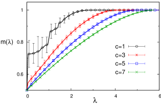
Figure 1: Numerical results for the averaged intensive index $m(\lambda)$ of Erdös-Rényi random graphs with the distribution of edges $P(J)=\delta(J-1)$, obtained using the population dynamics algorithm (solid lines) with $M=10^{6}$ random variables and $\epsilon=10^{-3}$. Numerical diagonalization results (symbols), calculated from an ensemble of $100$ matrices of size $N=3200$, are shown as a comparison.

The results for the prefactor $\sigma^{2}(\lambda)$ of ER random graphs are shown in figure 2. For the smaller values of $c$, the index fluctuations are generally stronger and $\sigma^{2}(\lambda)$ exhibits an irregular behavior, both features related to strong sample to sample fluctuations of the graph structure close to the percolation critical point. The prominent feature of figure 2 is that $\sigma^{2}(\lambda)$ shows a non-monotonic behavior, with a maximum for a certain intermediate value of $\lambda$ and a vanishing behavior at $\lambda=0$, which signals the breakdown of the linear scaling $\langle K^{2}\rangle-\langle K\rangle^{2}\propto N$. This is confirmed by the numerical diagonalization results of figure 3, where $\langle K^{2}\rangle-\langle K\rangle^{2}$ is calculated as a function of $N$ for $c=3$.

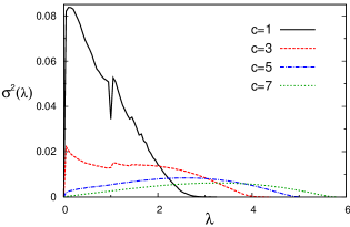
Figure 2: Numerical results for the prefactor $\sigma^{2}(\lambda)$ of the index variance of Erdös-Rényi random graphs with the distribution of edges $P(J)=\delta(J-1)$, obtained using the population dynamics algorithm with $M=10^{6}$ random variables and $\epsilon=10^{-3}$.

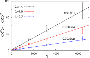
(a) Index variance for $\lambda>0$. The solid lines represent the linear fit $\langle K^{2}\rangle-\langle K\rangle^{2}=a+bN$, with the values of the slope $b$ indicated next to each straight line. The theoretical values for $\sigma^{2}(\lambda)$, calculated through the numerical solution of eq. (36), are given by $\sigma^{2}(0.5)=0.015$, $\sigma^{2}(3.0)=0.0085$ and $\sigma^{2}(3.5)=0.0040$.

(b) Index variance for $\lambda=0$. The solid line represents the logarithmic fit $\langle K^{2}\rangle-\langle K\rangle^{2}=a+b\ln N$, with the slope $b=0.47(6)$.

Figure 3: Numerical diagonalization results for the index variance of Erdös-Rényi random graphs with $c=3$ as a function of the number of nodes $N$. Each data point is calculated from an ensemble with $S$ independent realizations of the adjacency matrix $A$, where $S$ has been chosen according to $S=\frac{3.2\times 10^{5}}{N}$. The solid lines represent the best fits of the numerical data.

The results of figure 3(a), for different values of $\lambda>0$, display a linear behavior for increasing $N$, with slopes in full accordance with the theoretical values for $\sigma^{2}(\lambda)$, as indicated on the caption. On the other hand, figure 3(b) shows that the index variance scales as $\langle K^{2}\rangle-\langle K\rangle^{2}\propto\ln N$ for $\lambda=0$, similarly to the behavior of rotationally invariant ensembles Cavagna et al. (2000); Majumdar et al. (2009, 2011); Majumdar and Vivo (2012); Marino et al. (2014).

VI.2 Random regular graphs

In the case of random regular graphs, the degree distribution is simply $p_{k}=\delta_{k,c}$ Wormald (1999), where $c>2$ is an integer. Firstly, let us consider the situation in which the values of the edges are fixed, i.e., their distribution reads $P(J^{\prime})=\delta(J^{\prime}-J)$, with $J\in\mathbb{R}$. In this case, eq. (29) has the following solution for arbitrary $\mu$

$$W_{\mu}(u,v)=\left(-\frac{g\,v}{g^{*}u}\right)^{\frac{\mu}{2\pi}}\delta\left(u-g\right)\delta\left(v+g^{*}\right),$$ (38)

where $g$ is a root of the algebraic equation

$$(c-1)J^{2}g^{2}-zg+1=0.$$ (39)

The quantity $g$ represents the diagonal elements of the resolvent on the cavity graph Metz et al. (2010); Biroli et al. (2010). Substituting eq. (38) in eq. (31) and using the above quadratic equation, we get

$$\mathcal{G}_{N}(\mu,\lambda)=\lim_{\epsilon\rightarrow 0^{+}}\exp{\left[i\mu Nm(z)\right]},$$ (40)

where

$$m(z)=\frac{1}{\pi}{\rm Im}\left[\ln{\left(z-cJ^{2}g\right)}\right]-\frac{c}{2\pi}{\rm Im}\left[\ln{\left(1-J^{2}g^{2}\right)}\right].$$ (41)

Equation (40) is the large-$N$ behavior of $\mathcal{G}_{N}(\mu,\lambda)$ for random regular graphs in the absence of edge fluctuations. By choosing the proper roots of eq. (39) in the different sectors of the spectrum Metz et al. (2014), we can perform the limit $\lim_{\epsilon\rightarrow 0^{+}}m(z)$ and derive the following analytical result for $\lambda\geq 0$

$$m(\lambda) =1+\frac{1}{\pi}\tan^{-1}{\left[\frac{-c\sqrt{\lambda_{b}^{2}-\lambda^{2}}}{\lambda(c-2)}\right]}$$

$$-\frac{c}{2\pi}\tan^{-1}{\left[\frac{\lambda\sqrt{\lambda_{b}^{2}-\lambda^{2}}}{\lambda^{2}-2c(c-1)J^{2}}\right]},$$ (42)

with $|\lambda_{b}|=2|J|\sqrt{c-1}$ denoting the band edge of the continuous spectrum of random regular graphs Kesten (1959); McKay (1981). Equation (42) coincides with the average integrated density of states in the bulk of a Cayley tree Derrida and Rodgers (1993) and it converges to the result for the GOE ensemble when $c\gg 1$ Cavagna et al. (2000), as long as we rescale $J$ according to $J\rightarrow J/\sqrt{c}$. The substitution of eq. (40) in eq. (7) yields a delta peak $\mathcal{P}_{N}(K,\lambda)=\delta\left[K-Nm(\lambda)\right]$, which implies that $\sigma^{2}(\lambda)=0$. This suggests that the index variance exhibits the logarithmic scaling $\langle K^{2}\rangle-\langle K\rangle^{2}\propto\ln N$ for arbitrary $\lambda$. The latter property is consistent with the absence of localized states and the corresponding repulsion between nearest-eigenvalues, which is common to the whole spectrum of random regular graphs with uniform edges Jakobson et al. (1999); Oren and Smilansky (2010); Geisinger (2013).

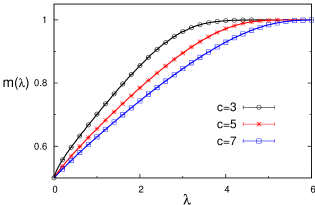
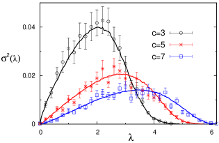
Figure 4: Numerical results for the averaged intensive index $m(\lambda)$ and the prefactor $\sigma^{2}(\lambda)$ of the index variance of random regular graphs with edges drawn from the Gaussian distribution $P(J)=\left(2\pi\right)^{-\frac{1}{2}}\exp{\left(-J^{2}/2\right)}$, obtained using the population dynamics algorithm (solid lines) with $M=5\times 10^{5}$ random variables and $\epsilon=10^{-3}$. Numerical diagonalization results (symbols), calculated from an ensemble of $100$ matrices of size $N=4000$, are shown as a comparison.

The above results are clearly due to our trivial choice for $P(J)$. The spectrum of random regular graphs contains localized states in the presence of edge disorder Kühn (2008); Bapst and Semerjian (2011) and one can expect that $\sigma^{2}(\lambda)$ exhibits a nontrivial behavior as long as $P(J)$ has a finite variance. The functions $m(\lambda)$ and $\sigma^{2}(\lambda)$ for random regular graphs with an arbitrary distribution $P(J)$ read

$$m(\lambda)=\frac{i}{2\pi}\lim_{\epsilon\rightarrow 0^{+}}\left[\frac{c}{2}K_{1}(z)-L_{1}(z)\right],$$

$$\sigma^{2}(\lambda)=\frac{1}{4\pi^{2}}\lim_{\epsilon\rightarrow 0^{+}}\Bigg{\{}\frac{c}{2}K_{2}(z)-\frac{c}{2}\left[K_{1}(z)\right]^{2}$$

$$\qquad\qquad\qquad\qquad+\left[L_{1}(z)\right]^{2}-L_{2}(z)\Bigg{\}},$$ (43)

where $K_{n}(z)$ and $L_{n}(z)$ are calculated from

$$K_{n}(z) =\int du\,dv\,du^{\prime}\,dv^{\prime}Q_{0}(u,v|c-1)Q_{0}(u^{\prime},v^{\prime}|c-1)$$

$$\times\left\langle\left[F_{J}(u,v;u^{\prime},v^{\prime})\right]^{n}\right\rangle_{J},$$

$$L_{n}(z) =\int du\,dv\,Q_{0}(u,v|c)\left[\ln{\left(-\frac{v}{u}\right)}\right]^{n}.$$ (44)

Figure 4 shows population dynamics results for $m(\lambda)$ and $\sigma^{2}(\lambda)$ in the case of a Gaussian distribution $P(J)=\left(2\pi\right)^{-\frac{1}{2}}\exp{\left(-J^{2}/2\right)}$. The function $m(\lambda)$ does not display any noticeable discontinuity, as observed previously for ER random graphs, due to the absence of disconnected clusters in the case of large random regular graphs Wormald (1999). In addition, we note that $\sigma^{2}(\lambda)$ has qualitatively the same non-monotonic behavior as in ER random graphs, exhibiting a maximum for a certain $\lambda$ and approaching zero as $\lambda\rightarrow 0$. Numerical diagonalization results for large matrices $A$, also shown in figure 4, confirm the correctness of our theoretical approach.

VI.3 The index distribution

In this subsection, we inspect the full index distribution of random graphs using numerical diagonalization, instead of undertaking the more difficult task of calculating the characteristic function from the numerical solution of eqs. (29) and (31). We restrict ourselves to $\lambda>0$, where the index variance scales linearly with $N\gg 1$.

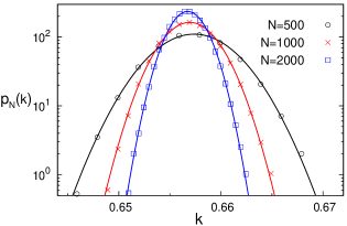
(a) Erdös-Rényi random graphs with the distribution of the edges $P(J)=\delta(J-1)$.

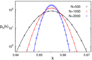
(b) Regular random graphs with the distribution of the edges $P(J)=\left(2\pi\right)^{-\frac{1}{2}}\exp{\left(-J^{2}/2\right)}$.

Figure 5: Numerical diagonalization results (symbols) for the distribution of the intensive index of random graphs with $c=5$ and $\lambda=1$. The histograms were generated from $10^{5}$ independent samples for the intensive index of the adjacency matrix $A$. The solid lines are Gaussian distributions with mean and variance taken from the data.

In figure 5 we show results for the distribution $p_{N}(k,\lambda)$ of the intensive index $k_{N}(\lambda)=\mathcal{K}_{N}(\lambda)/N$ in the case of ER and random regular graphs with $c=5$, obtained from numerical diagonalization for $\lambda=1$. For each value of $N$, the results are compared with a Gaussian distribution (solid lines) with mean and variance taken from the data, which confirms the Gaussian character of the typical index fluctuations for both random graph models when $N$ is large but finite.

Overall, our results suggest that, for $N\gg 1$ and $|\lambda|>0$, the intensive index of ER and random regular graphs is distributed according to

$$p_{N}(k,\lambda)=\sqrt{\frac{N}{2\pi\sigma^{2}(\lambda)}}\exp{\Bigg{\{}-\frac{N}{2\sigma^{2}(\lambda)}\left[k-m(\lambda)\right]^{2}\Bigg{\}}},$$ (45)

with non-universal parameters $\sigma^{2}(\lambda)$ and $m(\lambda)$ that depend on the underlying random graph model as well as on the particular value of the threshold $\lambda$. The function $p_{N}(k,\lambda)$ converges to $p_{N}(k,\lambda)=\delta{\left[k-m(\lambda)\right]}$ for $N\rightarrow\infty$, but the rate of convergence is slower when compared to rotationally invariant ensembles Cavagna et al. (2000); Majumdar et al. (2009, 2011); Majumdar and Vivo (2012); Marino et al. (2014), due to the logarithmic scaling of the index variance with respect to $N$ in the latter case. On the other hand, the Gaussian nature of the index fluctuations for $N\gg 1$ seems to be an ubiquitous feature of random matrix models.

VII Final remarks

We have presented an analytical expression for the characteristic function of the index distribution describing a broad class of random graph models, which comprises graphs with arbitrary degree and edge distributions. Ideally, this general result gives access to all moments of the index distribution in the limit $N\rightarrow\infty$. We have shown that the index variance of typical fluctuations is generally of $O(N)$, with a prefactor $\sigma^{2}(\lambda)$ that depends on the random graph model under study as well as on the threshold $\lambda$ that defines the index through eq. (3). In particular, $\sigma^{2}(\lambda)$ follows an intriguing non-monotonic behavior for random graphs with localized eigenstates: it exhibits a maximum at a certain $|\lambda|>0$ and a vanishing behavior at $\lambda=0$. Numerical diagonalization data confirm the theoretical results and support the Gaussian form of the typical index distribution for the random graphs considered here (see eq. (45)), completing the picture about the index statistics.

Our results differ with those of rotationally invariant ensembles, where the index variance is of $O(\ln N)$, with a prefactor that is independent of $\lambda$ and has an universal character. We argue that this difference in the scaling forms arises due to the presence of localized states in the spectrum of some random graphs. In the localized sectors, the eigenvalues do not repel each other and behave as uncorrelated random variables, such that the total number of eigenvalues contained in finite regions within the localized phase suffers from stronger finite size fluctuations as compared to regions within the extended phase, where level-repulsion tends to equalize the space between neighboring eigenvalues. On the other hand, the Gaussian nature of typical index fluctuations seems to be a robust feature of random matrix models.

On the methodological side, the replica approach as devised here departs from the representation of the characteristic function in terms of real Gaussian integrals, instead of the fermionic Gaussian integrals adopted in reference Cavagna et al. (2000). In the situations where $\sigma^{2}(\lambda)=0$, the logarithmic scaling of the index variance is obtained in our setting from the next-to-leading order terms, for large $N$, in the saddle-point integral of eq. (22). These contributions come from $O(1/\sqrt{N})$ fluctuations of the order-parameter and they are handled following the ideas of reference Metz et al. (2014). Indeed, we have precisely recovered the analytical results for the GOE ensemble Cavagna et al. (2000) employing this strategy Metz (2014), and the same approach can be used to calculate the prefactors in situations where the variance of random graphs is of $O(\ln N)$.

Our work opens several perspectives in the study of the typical index fluctuations. Firstly, it would be worth having approximate schemes or numerical methods to solve eq. (29) and obtain the distribution $W_{\mu}(u,v)$, which would allow to fully determine the characteristic function for random graphs. Due to the versatile character of the replica method, the study of the averaged integrated density of states of the Anderson model on regular graphs Abou-Chacra et al. (1973) and its sample to sample fluctuations is just around the corner. It would be also interesting to inspect the robustness of the Gaussian form of the index fluctuations in random matrix ensembles with strong inherent fluctuations, such as Levy random matrices Cizeau and Bouchaud (1994) and scale-free random networks Barabási and Albert (1999). The index statistics of both random matrix models can be treated using the replica approach as developed here. In fact, scale-free random graphs, crucial in modelling many real-world networks appearing in nature Barrat et al. (2008), can be studied directly from our work by choosing the degree distribution as $p_{k}\sim k^{-\gamma}$ ($2<\gamma\leq 3$), which yields random graphs with strong sample to sample degree fluctuations. Finally, we point out that the different scaling behaviors of the index variance should have important consequences to the relaxation properties and search algorithms on complex energy surfaces.