The Center of Light: Spectroastrometric Detection of Exomoons

Abstract

Direct imaging of extrasolar planets with future space-based coronagraphic telescopes may provide a means of detecting companion moons at wavelengths where the moon outshines the planet. We propose a detection strategy based on the positional variation of the center of light with wavelength, “spectroastrometry.” This new application of this technique could be used to detect an exomoon, to determine the exomoon’s orbit and the mass of the host exoplanet, and to disentangle of the spectra of the planet and moon. We consider two model systems, for which we discuss the requirements for detection of exomoons around nearby stars. We simulate the characterization of an Earth-Moon analog system with spectroastrometry, showing that the orbit, the planet mass, and the spectra of both bodies can be recovered. To enable the detection and characterization of exomoons we recommend that coronagraphic telescopes should extend in wavelength coverage to 3 micron, and should be designed with spectroastrometric requirements in mind.

1. Introduction

Techniques and ideas for detecting moons orbiting exoplanets have progressed rapidly in the last decade. These advances are driven, at least in part, by a desire to extend our understanding of satellite formation and origins to cases beyond the Solar System. For example, while the formation of moons and/or moon systems may be common around giant planets, there exist many physical models for this process (Lunine & Stevenson, 1982; Canup & Ward, 2002; Mosqueira & Estrada, 2003; Ogihara & Ida, 2012). Additionally, the likelihoods of satellite formation by giant impact (Hartmann & Davis, 1975; Cameron & Ward, 1976) and capture (McCord, 1966; McKinnon, 1984) remain uncertain (e.g., Agnor & Asphaug, 2004; Agnor & Hamilton, 2006).

Exomoons can be potentially habitable targets in their own right, and may also affect the habitability and characterization of the host planet (Heller et al., 2014). Habitable, Earth-like moons orbiting gas giant planets in circumstellar habitable zones have been proposed (Williams et al., 1997; Kaltenegger, 2000) and discussed (Scharf, 2006; Heller, 2012; Heller & Barnes, 2013; Heller & Pudritz, 2015a; Heller & Barnes, 2015; Hinkel & Kane, 2013; Duncan & Kipping, 2013; Kaltenegger, 2010; Heller & Armstrong, 2014; Reynolds et al., 1987). For rocky planets in the habitable zone, the undetected presence of a large satellite can confuse characterization attempts, as the moon is an additional source of thermal or reflected light (Robinson, 2011), potentially with its own molecular features (Rein et al., 2014). Detecting large companions could also aid in the characterization of potentially habitable exoplanets, as large satellites can help provide long-term obliquity, and thus climate, stability (Laskar et al., 1993). However, the presence of large moons does not necessarily imply such stability (Ward et al., 2002), nor is a moon necessitated for moderate obliquity stability (Lissauer et al., 2012), and it might reduce habitability near the outer edge of the insolation habitable zone (Armstrong et al., 2014).

Given the importance of satellites to exoplanet characterization and in advancing our understanding of planet formation models, it is not surprising that many techniques for exomoon detection have been proposed. Most techniques have focused on analyzing exoplanet transit timing and/or duration signals (Sartoretti & Schneider, 1999; Szabó et al., 2006; Simon et al., 2007; Kipping, 2009), which can vary due to the orbit of the planet about the planet-moon barycenter. Additionally, mutual events, with a moon occulting its host star or planet while the planet transits the star, as well as the overlap of the moon and planet during transit, can cause photometric variations in the stellar signal (Sartoretti & Schneider, 1999; Szabó et al., 2006; Kipping, 2011; Tusnski & Valio, 2011; Heller, 2014), while spectroscopy during the transit of an exomoon that is well separated from its companion planet might allow for a measurement of the exomoon’s atmospheric transmission spectrum (Kaltenegger, 2010). Most of these effects have been considered in an ongoing search for exomoons in the Kepler dataset (Kipping et al., 2012).

By comparison, relatively few techniques have been developed that are relevant to direct observations of exoplanets, where the planet is resolved from the host star in either reflected or emitted light. Development of such techniques is prudent given the near- and long-term interest in exoplanet direct imaging and characterization (Kouveliotou et al., 2014; Stapelfeldt et al., 2014; Spergel et al., 2015). Cabrera & Schneider (2007) discussed using mutual transit and shadowing effects to detect a moon in an unresolved planet-moon system, which is made difficult by requiring an observational duty cycle near to 100% of the moon’s orbit and/or a fortuitous inclination of the moon’s orbit relative to the observer. Moskovitz et al. (2009) discussed the influence of a large moon on the bolometric thermal-infrared phase curve of its host planet, and Robinson (2011) suggested that phase-dependent variability at wavelengths corresponding to strong absorption bands for the host planet could indicate the presence of an airless moon. Recently, Peters & Turner (2013) discussed the direct detection of tidally-heated exomoons, which can be made to be very luminous depending on the amount of input tidal energy.

A major obstacle to exomoon detection in direct observations of exoplanets is angular resolution. For example, at a distance of 1.34 pc ($\alpha$ Cen system) the Earth-Moon angular separation would span 1.9 mas, and the Saturn-Titan angular separation at that same distance would be 6.0 mas. Thus, to resolve these pairs of worlds, a telescope operating in V-band would need to have a diameter of about 25 m or more, and this value increases to be on the order of a kilometer at 10 $\mu$m in the thermal infrared.

Here, we turn to a mature technique in observational astronomy, spectroastrometry (Bailey, 1998; Whelan & Garcia, 2008), as a new means for detecting exomoons in direct observations of exoplanets. In spectroastrometry, the wavelength-dependent shift in the light centroid of an unresolved source can be used to indicate the presence of an unresolved companion body and to yield orbital parameters of the companion. This is limited by the optical design and diffraction within the telescope, which spread a point source of light into a broadened distribution of photons, referred to as the “point spread function,” or PSF. A spectroastrometric detection is made possible by the angular shift of the PSF centroid with wavelength, which can be measured to precisions better than the angular resolution of the telescope, which sets the size of the PSF, yielding information at the angular scale of the exoplanet-exomoon separation.

We propose a new technique to detect exomoons using a high-contrast imaging coronagraph which suppresses the light of the host star exterior to an inner working angle (e.g. Guyon et al., 2006; Stapelfeldt et al., 2014), enabling direct imaging of the unresolved exoplanet and exomoon. This can alternately be accomplished with an external star shade (Cash, 2006). At wavelengths where the exoplanet dominates the flux, the centroid will approach the position of the exoplanet, while at wavelengths where the exomoon dominates, the centroid will approach the position of the exomoon (Figure 1). Spectroastrometry then allows for the measurement of the centroid shift of the PSF containing the exoplanet and its moon, resulting in the detection of the exomoon, as well as enabling follow-up observations for characterization of the star-planet-moon system. This technique works optimally for an instrument that is capable of measuring both spatial and spectral information simultaneously, although we do not specify the detector design in this study.

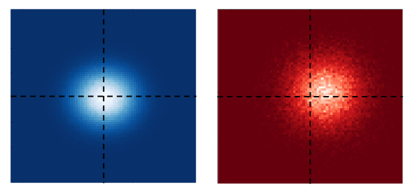
Figure 1.— Spectroastrometric signal. Left: at a bluer wavelength dominated by the planet, the centroid aligns with the planet’s position at the origin. Right: at a redder wavelength dominated by the moon (within an absorption band in which the planet’s spectrum is dark), the centroid shifts to the position of the moon.

We begin this paper with a discussion of our spectral models for the planets and moons (§2). Next, we discuss the methods of our simulations (§3), starting with the fiducial model parameters of the systems we study (§3.1), the definition of spectroastrometric signal (§3.2), the computation of the signal-to-noise for detection of a moon (§3.3), and finishing with a description of Monte Carlo simulations of spectroastrometric observations (§3.4). Next, we present results of the optimization of wavelength choice for detection (§4.1), and an example of the characterization of a hypothetical nearby planet-moon system with spectroastrometry (§4.2). We discuss how our results will scale with the various assumed parameters (§4.3). We end with a discussion and conclusions.

2. Description of Spectral Models

We use two fiducial model systems to explore the prospects for spectroastrometry: an Earth-Moon twin around the star Alpha Centauri A ($\alpha$ Cen A; 1.34 parsecs), and an Earth-Jovian analog at 1 AU around a G2V (sun-like) star at 10 parsecs (Table 1). We use three distinct planet spectral models to simulate the spectra of an exo-Earth, an exo-Moon, and a warm Jupiter (i.e., a Jupiter-like planet at an orbital distance of 1-2 AU from a Sun-like star). Our Earth and Moon models are described in the following subsections. The spectrum of the warm Jupiter was generated by the radiative-convective models described in Burrows et al. (2004) and Sudarsky et al. (2003). These models produce phase-averaged spectra of irradiated gas giants for a set of assumed elemental abundances, and include the effects of cloud condensation and multiple scattering. The atmosphere in these models is assumed to be planar, and the particular model that we use in this work is for a solar-composition, Jupiter-mass planet orbiting a G2V star at a distance of 1 AU. The jovian’s atmosphere is taken to be in chemical equilibrium, and the equilibrium abundances of key atmospheric trace gases are computed according to Burrows & Sharp (1999).

Table 1The moon and planetary parameters used in our model, where $D_{tele}$ is the telescope diameter, d is the distance from the observer, $t_{obs}$ is the duration of exposure, $\epsilon$ is the telescope efficiency factor.

Moon radius Planet radius Planet-moon Orbital $D_{tele}$ d $t_{obs}$ $\epsilon$ Semi-major System (m) (m) separation (m) period (d) (m) (pc) (hr) axis (AU) Earth-Moon 1.738$\times 10^{6}$ 6.371$\times 10^{6}$ 3.844$\times 10^{8}$ 27.32 12 1.34 24 0.2 1.23 Jovian-Earth 6.371$\times 10^{6}$ 6.991$\times 10^{7}$ 3.064$\times 10^{9}$ 34.60 12 10 24 0.2 1

2.1. Earth Spectrum Model

To simulate Earth’s disk-integrated spectrum, we use the NASA Astrobiology Institute’s Virtual Planetary Laboratory three-dimensional, multiple scattering spectral Earth model, which generates temporally and spectrally resolved disk-integrated synthetic observations of Earth. This model has been described and extensively validated both for temporal variability and for a variety of phases, at wavelengths from the near-ultraviolet through the IR in previous papers (Robinson et al., 2010, 2011; Robinson et al., 2014), so only a brief description of the model is presented here.

In our simulations, we divide Earth into a number of equal area pixels according to the HEALPix scheme (Górski et al., 2005), and Earth’s disk-integrated spectrum is computed by summing the radiances coming from the pixels on the observable hemisphere. The wavelength-dependent radiance coming from any given pixel is assembled from a lookup table that contains spectra generated over a grid of different solar and observer zenith and azimuth angles. Elements within the lookup table, which are generated using a one-dimensional, line-by-line radiative transfer model (Meadows & Crisp, 1996), are computed for a variety of different surface and atmospheric conditions, as well as several different cloud coverage scenarios (e.g., thick, low cloud or thin, high cloud).

To simulate time-dependent changes in Earth’s spectrum we use spatially-resolved, date-specific observations of key surface and atmospheric properties from Earth observing satellites as input to our Earth model. Gas mixing ratio and/or temperature profiles are taken from the Microwave Limb Sounder (Waters et al., 2006), the Tropospheric Emission Spectrometer (Beer et al., 2001), the Atmospheric Infrared Sounder (Aumann et al., 2003), and the CarbonTracker project (Peters et al., 2007). Snow cover and sea ice data as well as cloud cover and optical thickness data are taken from the Moderate Resolution Imaging Spectroradiometer instruments (Salomonson et al., 1989) aboard NASA’s Terra and Aqua satellites (Hall et al., 1995; Riggs et al., 1999). Wavelength-dependent optical properties for liquid water clouds were derived using a Mie theory model (Crisp, 1997) and were parametrized using geometric optics for ice clouds (Muinonen et al., 1989). The spectra presented in this work are for Earth at northern vernal equinox at quadrature phase.

2.2. Moon Spectrum Model

We divide the Moon’s spectrum into two components: reflected solar and emitted thermal. At quadrature, the reflected component dominates at wavelengths below 3.5 $\mu$m and the emitted component dominates at wavelengths above this. The thermal component of the spectrum is computed using the model presented in Robinson (2011). The model generates phase-dependent, thermal infrared spectra of the Moon assuming globally-averaged values of the lunar Bond albedo, nightside temperature, and the spectrally-resolved surface emissivity.

The lunar phase function is markedly non-Lambertian, so we use empirical models of the Moon’s phase-dependent reflectivity to simulate the shortwave component of the lunar spectrum. Spectrally-resolved measurements of the lunar surface phase function from the RObotic Lunar Observatory (ROLO) are used to simulate the reflected light component of the lunar spectrum at star-planet-observer angles (i.e., phase angles) between 0^∘ and 97^∘, which are the phase angles for which the surface phase function has been published (Buratti et al., 2011). The ratio of the specific intensity emerging from a surface element ($I_{\lambda}(\alpha,\mu_{0},\mu)$, where $\alpha$ is the phase angle, and $\mu_{0}$ and $\mu$ are the cosines of the incident solar angle and the emission angle, respectively) to the incident specific solar flux ($F_{\lambda}=F_{\sun}/\pi$) is given by (Chandrasekhar, 1960),

$$I_{\lambda}(\alpha,\mu_{0},\mu)/F_{\lambda}=f(\alpha)[\mu_{0}/(\mu+\mu_{0})]\ ,$$ (1)

where $f(\alpha)$ is the surface solar phase function (which is distinct from the planetary phase function), and the final collection of terms in brackets provides the functional form of the lunar scattering law. The ROLO data provide $f(\alpha)$, so that we can integrate $I_{\lambda}(\alpha,\mu_{0},\mu)$ from Eq. 1 over the illuminated disk, which eliminates the dependence on $\mu_{0}$ and $\mu$, and allows us to compute the phase-dependent, reflected light spectrum of the Moon, $I_{\lambda}(\alpha)$.

At phase angles larger than 97^∘, where $f(\alpha)$ is not reported, we model the Moon’s reflected light spectrum using the lunar phase functions of Lane & Irvine (1973), who measured the Moon’s brightness over a wide range of phases through a series of broadband filters from the near-ultraviolet to the near-infrared. By pairing these measurements of the Moon’s phase function with a medium-resolution ($\lambda/\Delta\lambda\sim$ 500) measurement of the disk-integrated lunar spectrum from NASA’s EPOXI mission (Livengood et al., 2011), we can infer the Moon’s spectrum at phase angles other than that at which the EPOXI data were acquired. Thus, for large phase angles, we take the phase-dependent, disk-integrated specific brightness of the Moon to be

$$I_{\lambda}(\alpha)=I_{\lambda}(\alpha^{\prime})\frac{\Phi(\alpha)}{\Phi(\alpha^{\prime})}\ ,$$ (2)

where $\alpha^{\prime}$ is the phase angle of the EPOXI observations, and $\Phi$ is the planetary phase function measured by Lane & Irvine (1973). The lunar EPOXI observations span 0.3 $\mu$m to about 4.5 $\mu$m in wavelength, and were taken at a phase angle of 75.1^∘. In general, our two approaches to simulating the reflected-light component of the Moon’s spectrum agree to within measurement error at phase angles near quadrature, $\alpha=90^{\circ}$, which is the phase that we emphasize in this work.

3. Methods

The spatial resolution needed to detect the spectroastrometric signal for our fiducial simulated planet-moon systems is much greater than any telescope can currently provide, and greater than the proposed first-generation direct imaging missions. Both planet-moon systems have a separation of $\approx 2$ milliarcseconds (mas), while the Hubble Space Telescope has a PSF width of $\approx$100 mas at 2.5 micron (and no coronagraph), and first-generation imaging telescopes will have similar spatial resolutions. Consequently we focus on future second-generation telescopes. To simulate a spectroastrometric detection of the exomoon models presented in this paper, we explored the multidimensional parameter space of an idealized coronagraphic space telescope capable of such a feat. A space telescope would be ideal for exomoon detection due to the ability to observe in the Earth’s atmospheric windows and to avoid atmospheric turbulence without the aid of adaptive optics; these same requirements apply to coronagraphic detection and characterization of Earth-like planets in their habitable zones. In §3.1 we outline the parameters used in our model, in §3.2 we define the spectroastrometric signal, in §3.3 we discuss the photon-limited noise and signal-to-noise, and in §3.4 we describe Monte Carlo simulations of spectroastrometric observations.

3.1. Model System Parameters

We have assumed a planet-moon system whose moon orbits in the planet’s equatorial plane in prograde motion. The planet-moon separation for the ExoEarth-Moon system was taken to be the current Earth-Moon separation, while the separation for the Jovian-Earth system was taken to be 30$\%$ of the Hill radius of a warm Jupiter at 1 AU from a Sun-like star (corresponding to 43 $R_{Jupiter}$), slightly less than the critical semi-major axis for a prograde satellite (Barnes & O’Brien, 2002). For the preliminary exploration of the signal-to-noise ratio for different spectral resolutions and wavelength pairs, we set the telescope diameter to 12 meters, distance to the system from the observer to 1.34 parsecs (Earth-Moon) and 10 pc (Jovian-Earth), and exposure time to 1 day (Table 1). We assume that the moon-planet position is fixed over the range of the exposure; since both of our fiducial systems have orbital periods of $\approx 30$ days, the centroid will shift by $\approx 12^{\circ}$ over this time, which is only 20% of the planet-moon separation, and a very small fraction of the width of the PSF. We have selected a 12-meter telescope based on the range of apertures being considered for the “High-Definition Space Telescope” (HDST; Dalcanton et al., 2015), which is informed by a (conservative) estimate of the detectability of Earth-like planets (Stark et al., 2015). The telescope efficiency factor, which accounts for instrument throughput, detector quantum efficiency, and photometric aperture losses, was kept at 20$\%$ throughout all calculations. These system parameters may be found in Table 1. Section §4.3 explores the effect that varying the telescope size and distance from the observer has on the signal to noise ratio.

Such a large telescope would be capable of rapid detection of Earth-sized exoplanets (in of order a few weeks) with a direct-imaging survey of nearby Sun-like stars (Agol, 2007). The planets found with this initial coronagraphic imaging survey could then be prioritized based upon, for example, their presence within their host-star habitable zone and potential for the existence of a large, detectable exomoon, to motivate the additional observing time for detailed spectral and spectroastrometric characterization.

We note that the parameters of the Jovian-Earth model system we have chosen are driven by favorable observational detectability rather than theoretical prejudice. Models of satellite formation around giant planets have been tailored for the Solar System to reproduce, for example, the mass ratio of $10^{-4}$ observed for the satellite systems of the giant planets (Canup & Ward, 2002; Sasaki et al., 2010), so that giant planets may harbor satellites as large as $0.7R_{\oplus}$ (Heller & Pudritz, 2015b). In addition, models of in-situ formation of satellites from a disk produce regular satellites at distances of $6-30R_{Jupiter}$. Thus, within the context of these models, an Earth-sized satellite at 43 $R_{Jupiter}$ distance from a giant planet is unexpected, but may have formed by other means, including capture and migration.

3.2. Spectroastrometric Signal

The spectroastrometric signal is the difference in the centroid positions when the system is observed at two different wavelengths. We define the centroid position, ${\bf c}(\lambda)$, as being the flux-weighted center of light of the planet and moon as a function of wavelength, $\lambda$, in the direction of two angular sky coordinates, $(x,y)$, which we denote as ${\bf c}(\lambda)=(c_{x}(\lambda),c_{y}(\lambda))$, where $c_{x,y}$ are the $(x,y)$ centroids with respect to the origin of the star-planet-moon system (and the orientation of the coordinates is chosen with respect to an observer-defined reference direction). Note that the angular coordinates $(x,y)$ are expressed in milliarcseconds (mas), which is the typical order of the moon-planet separation.

The detector will be capable of measuring this signal over a wave band with central wavelength $\lambda$ and spectral resolution $R$, giving the width of the band $\Delta\lambda=\lambda/R$. We define the band-averaged centroid as

$$\bar{\bf c}(\lambda)=\frac{\int_{\lambda-\Delta\lambda/2}^{\lambda+\Delta\lambda/2}{\bf c}(\lambda)\lambda F_{\lambda}d\lambda}{\int_{\lambda-\Delta\lambda/2}^{\lambda+\Delta\lambda/2}\lambda F_{\lambda}d\lambda},$$ (3)

where $F_{\lambda}$ is the total flux of the planet and moon, and we have weighted the centroid by the number of photons detected.

In computing the model centroid, we define $F_{m,\lambda}$ and $F_{p,\lambda}$ to represent the flux of the moon and the planet, respectively, and ${\bf r}_{m}$ and ${\bf r}_{p}$ to represent the positions of these bodies (in two dimensions, projected onto the sky plane, perpendicular to our line of sight). The position of the wavelength-dependent centroid, ${\bf c}(\lambda)$, is

$${\bf c}({\lambda}) = \frac{F_{m,\lambda}{\bf r}_{m}+F_{p,\lambda}{\bf r}_{p}}{d(F_{m,\lambda}+F_{p,\lambda})}$$ (4)

$$= \frac{F_{m,\lambda}\vec{\beta}}{F_{m,\lambda}+F_{p,\lambda}}+\frac{{\bf r}_{p}}{d}$$ (5)

where $\vec{\beta}=({\bf r}_{m}-{\bf r}_{p})/d$ is the angular sky separation between the moon and planet in radians at a distance $d$ from the observer (we convert this to milliarcseoconds). Note that this equation neglects the variation of the center of light of each body with the illumination phase; this is on the order of the angular size of each body, which is much smaller than the spectroastrometric signal.

Measuring ${\bf c}({\lambda})$ requires a reference position on the sky, for example the planet’s position, while the planet’s position is not known a priori in the presence of a centroid-shifting moon. However, knowledge of the planet’s position is not needed when considering only the difference between the centroids measured in different spectral bands. This is the spectroastrometric signal, $S(\lambda_{1},\lambda_{2})$, which scales as the scalar difference of the planet/moon centroid in two wave bands,

$$S(\lambda_{1},\lambda_{2})=|\bar{\bf c}(\lambda_{1})-\bar{\bf c}(\lambda_{2})|,$$ (6)

which we measure in milliarcseconds. Note that it may be possible to select a different resolution $R$ for each wave band. A significant advantage of measuring the spectroastrometric signal, $S(\lambda_{1},\lambda_{2})$, rather than ${\bf c}(\lambda)$ is that the absolute position of the planet-moon system does not need to be calibrated; only the relative position with wavelength needs to be measured. This obviates the need for an absolute sky coordinate reference frame, which can be a challenging measurement to make (although the host star could perhaps be used, as discussed below). Also, the position of the planet is affected by its orbit about the star, its illumination, its orbit about the center of mass with the moon, and its gravitational perturbation by companion planets; measurement of the spectroastrometric signal eliminates all of these confounding effects. Note that this technique does not require flux calibration since the spectroastrometric signal is normalized by the total flux of the planet and moon.

3.3. Signal to Noise Ratio of Detection

The spectroastrometric noise scales as the ratio of the width of the point spread function incident on the detector to the square root of the number of photons, assuming Poisson noise from the planet and moon dominates the uncertainty. In light of the extraordinary engineering called for in the success of this project, we have assumed that an ideal coronagraphic space telescope would produce negligible instrumental noise (due to the dark current, read noise, scattered light, pixel size, etc). We estimate the number of photons, $N(\lambda)$, incident on the coronagraph’s detector due to the planet and moon within a band of width $\Delta\lambda$ for some exposure time $t_{obs}$ to be

$$N(\lambda) = \pi\epsilon\frac{D^{2}_{tele}}{4}t_{obs}\int_{\lambda-\Delta\lambda/2}^{\lambda+\Delta\lambda/2}\frac{\lambda}{hc}F_{\lambda}d\lambda$$ (7)

$$\approx \pi\epsilon\frac{D^{2}_{tele}}{4}\frac{\Delta\lambda}{\lambda}\frac{\lambda^{2}}{hc}{t_{obs}}F_{\lambda},$$ (8)

where $\epsilon$ is the chosen efficiency factor of the telescope (defined as the fraction of all photons incident on the telescope aperture that are measured by the detector; we assume that it is wavelength-independent), $D_{tele}$ is the diameter of the telescope, $h$ the Planck constant, $c$ the speed of light, and $F_{\lambda}$ is the wavelength dependent flux density (the approximation assumes that this flux is roughly constant across a narrow band). A deeper analysis of this calculation can be found in Agol (2007); note that $R=\lambda/\Delta\lambda$ is the spectral resolving power.

We assume that the PSF of the planet is well approximated by an Airy disk, which we in turn approximate as a Gaussian with angular profile $I(\theta)\propto\exp{-\frac{1}{2}(\theta/\sigma_{PSF})^{2}}$, where $\sigma_{PSF}=0.45\lambda/D_{tele}$ is the angular size of the Airy disk, and $\theta$ is the angular coordinate from the center of the PSF. The precision of the measurement of the centroid improves with the square root of the number of photons detected. Thus, the spectroastrometric noise for an ideal (photon-noise limited) coronagraphic space telescope is then

$$\sigma(\lambda)=\frac{\sigma_{PSF}}{N(\lambda)^{1/2}}\approx\frac{0.45\lambda}{D_{tele}}\left(\pi\epsilon\frac{D^{2}_{tele}}{4}\frac{\Delta\lambda}{\lambda}\frac{\lambda^{2}}{hc}t_{obs}F_{\lambda}\right)^{-1/2}.$$ (9)

The spectroastrometric signal-to-noise ratio (hereafter SNR) we define as

$$\text{SNR}\equiv\frac{S(\lambda_{1},\lambda_{2})}{\sqrt{\sigma(\lambda_{1})^{2}+\sigma(\lambda_{2})^{2}}}$$ (10)

between two wavelengths $\lambda_{1}$ and $\lambda_{2}$. Below we set the threshold for exomoon detection in our model systems at a minimum 5$-\sigma$ confidence level, i.e. $SNR\geq 5$.

In practice, the noise is typically dominated by the moon wave band. This gives an approximate expression for the signal-to-noise ratio of

$$\text{SNR}\approx\beta\frac{D_{tele}}{0.45\lambda_{1}}\left(\pi\epsilon\frac{D^{2}_{tele}}{4}\frac{\Delta\lambda_{1}}{\lambda_{1}}\frac{\lambda_{1}^{2}}{hc}{t_{obs}}F_{\lambda_{1}}\right)^{1/2},$$ (11)

where we have assumed that $\lambda_{1}$ is dominated by the moon while $\lambda_{2}$ is dominated by the planet, and $\beta=|\vec{\beta}|$ is the moon-planet separation on the sky at the time of observation. Note that in the wave band dominated by the moon, $F_{\lambda}\propto(R_{m}/d)^{2}$, so overall the signal-to-noise scales as

$$SNR\propto a_{mp}R_{m}\left(\frac{D_{tele}}{d}\right)^{2}\left(\frac{\epsilon t_{obs}}{R}\right)^{1/2}\left(\frac{F_{\lambda_{1}}d^{2}}{\pi R_{m}^{2}}\right)^{1/2},$$ (12)

where $a_{mp}=|{\bf r}_{m}-{\bf r}_{p}|=\beta d$ is the sky-plane projected physical separation of the planet and moon, $R_{m}$ is the radius of the moon, and the last quantity in this equation is the disk-integrated specific intensity of the moon.

We use these equations below for estimation of the detectability of a moon-planet system, while for characterization of a detected system, we employ Monte Carlo simulations, described next.

3.4. Monte Carlo Simulations

We have carried out Monte Carlo simulations of coronagraphic observations of a detected moon-planet system with the same idealized assumptions: we assume a broad range of wavelength sensitivity, and we assume that the photon counting noise and diffraction limit can be achieved. We define spectral bins equally spaced in log wavelength between a minimum and maximum wavelength. For each spectral bin, we compute the predicted number of photons within the bin for each body, $N(\lambda)$, and then draw the observed number of photons from a Poisson distribution. We next add a random Gaussian deviate in both directions on the sky with a standard deviation of $\sigma(\lambda)=0.45\lambda/(D_{tele}N(\lambda)^{1/2})$ at the position of each body. We then compute the flux-weighted average positions of both bodies to obtain $\bar{\bf c}(\lambda)$, and compute the centroid uncertainty, $\sigma(\lambda)$, from a weighted mean of the individual bodies’ centroid uncertainties. The result of this is a total photon flux and $(x,y)$ centroid position for each spectral bin, ${\bf c}(\lambda)$, as well as the photon-noise limited uncertainty (which we assume to be the same in the $x-$ and $y-$ directions).

We have also run simulations in which we randomly draw individual photons from the spectral shapes of each body, and assign a position and positional uncertainty to each photon. We then bin these photons in wavelength to measure the spectrum, and compute the centroid within each bin to measure the spectroastrometric signal, $\bar{\bf c}(\lambda)$; we compute uncertainties on the photon flux from the square root of the number of photons in each bin, and on the centroid from the scatter in the photon positions divided by the square root of the number of photons in each bin. This approach is more time intensive, yet gives equivalent results to the pre-binned spectrum approach.

4. Results

Our results outline the range of instrumental, spectroscopic, and planetary system parameters for which we expect the spectroastrometric method to detect the presence of an exomoon. In §4.1, we discuss the optimum observing wavelengths and spectral resolutions found with telescope and planet-moon system parameters fixed at values described in §3.1. In §4.2 we give an example of characterization of an Earth-Moon twin at the distance of $\alpha$ Cen. In §4.3, we discuss the results of varying the distance and telescope size for both systems while spectral resolution and observing wavelengths are fixed at favorable values.

4.1. Optimum Spectral Resolutions and Observing Wavelengths for the Model Systems

Sections §4.1.1 and §4.1.2 discuss our particular model systems in more detail. Results for both systems reflect the inherent challenge of spectroastrometry: moon-dominated wavelengths tend to exist because the host planet is dim due to atmospheric absorption, not due to emission features of the moon. Thus, the bands with highest centroid offset inherently have less total flux and an elevated level of noise. In order to bring the SNR at these wavelengths above the detection threshold, a balance must be struck between a spectral resolution which is low enough to let in many photons, yet high enough to reveal a measurable shift in the centroid.

4.1.1 Moon-like Exomoon Orbiting an Earth-like Planet

In an Earth-Moon analog system, the Moon outshines the Earth in the water bands around 1.96 and 2.6 - 3.0 $\mu$m, the carbon dioxide band at 4.2 - 4.4 $\mu$m, and it has a sizable thermal excess around 5.0 - 8.0 $\mu$m (Fig. 2, top plot), although in this paper we only consider wavelengths out to 3 micron. The maximum fraction of the Moon’s flux for the Earth-Moon system occurs at $\lambda$ = 2.69 $\mu$m, contributing 99.8$\%$ to the total flux when viewed with spectral resolving power R = 100 (Fig. 2, bottom plot).

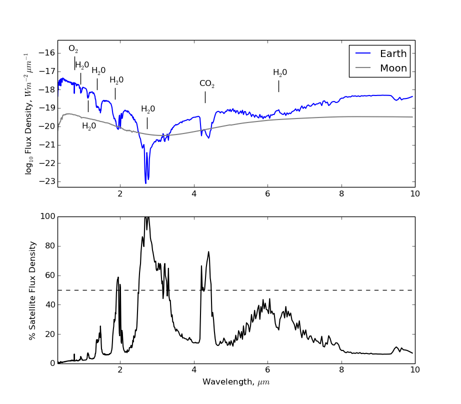
Figure 2.— The flux of a twin Earth-Moon system at quadrature phase angle orbiting $\alpha$ Cen A as a function of wavelength in microns (top) and the contribution of flux due to the moon shown as a fraction of the total flux (bottom). The maximum fraction of the moon’s flux for the Earth-Moon system occurs at $\lambda$ = 2.7 $\mu$m, contributing 99.8$\%$ to the total flux.

To optimize the spectroastrometric SNR requires choosing two wavelengths and resolutions at which the difference in centroid is large, but the noise is also small. At lower spectral resolution, the centroid offset, $\bar{c}(\lambda)$, becomes smoother so that the molecular absorption bands, at which the Moon dominates the flux, are averaged with wavelengths where the Earth dominates (Fig. 3). The noise decreases at lower spectral resolution due to the larger number of photons in each band, which compensates for the smoothing of the centroid offset. Consequently lower spectral resolution generally gives a higher signal-to-noise of detection.

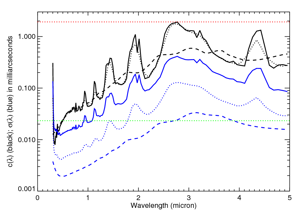
Figure 3.— The centroid offset, $c(\lambda)$, and uncertainty, $\sigma(\lambda)$ for an Earth-Moon twin at the distance of 1.34 pc ($\alpha$Cen; see Table 1 for simulation parameters). The reference position is the centroid of the planet ($c(\lambda)=0$ mas), while the moon is at $c(\lambda)=1.9$ mas (red dotted line) and the center of mass is at 0.023 mas (green dotted line). Black lines are $\bar{c}(\lambda)$, while blue are $\sigma(\lambda)$. Solid, dotted, and dashed black/blue lines correspond to $R=100,10,1$.

Our calculated SNR results for the Earth-Moon system at 1.34 pc exceed the 5$-\sigma$ detection threshold for the parameters listed in Table 1 for a wide range of wavelengths and resolutions (Table 2, Fig. 4). The optimal wavelengths cluster near $0.35$ micron and $2.7$ micron where the planet and the moon dominate the flux, respectively.

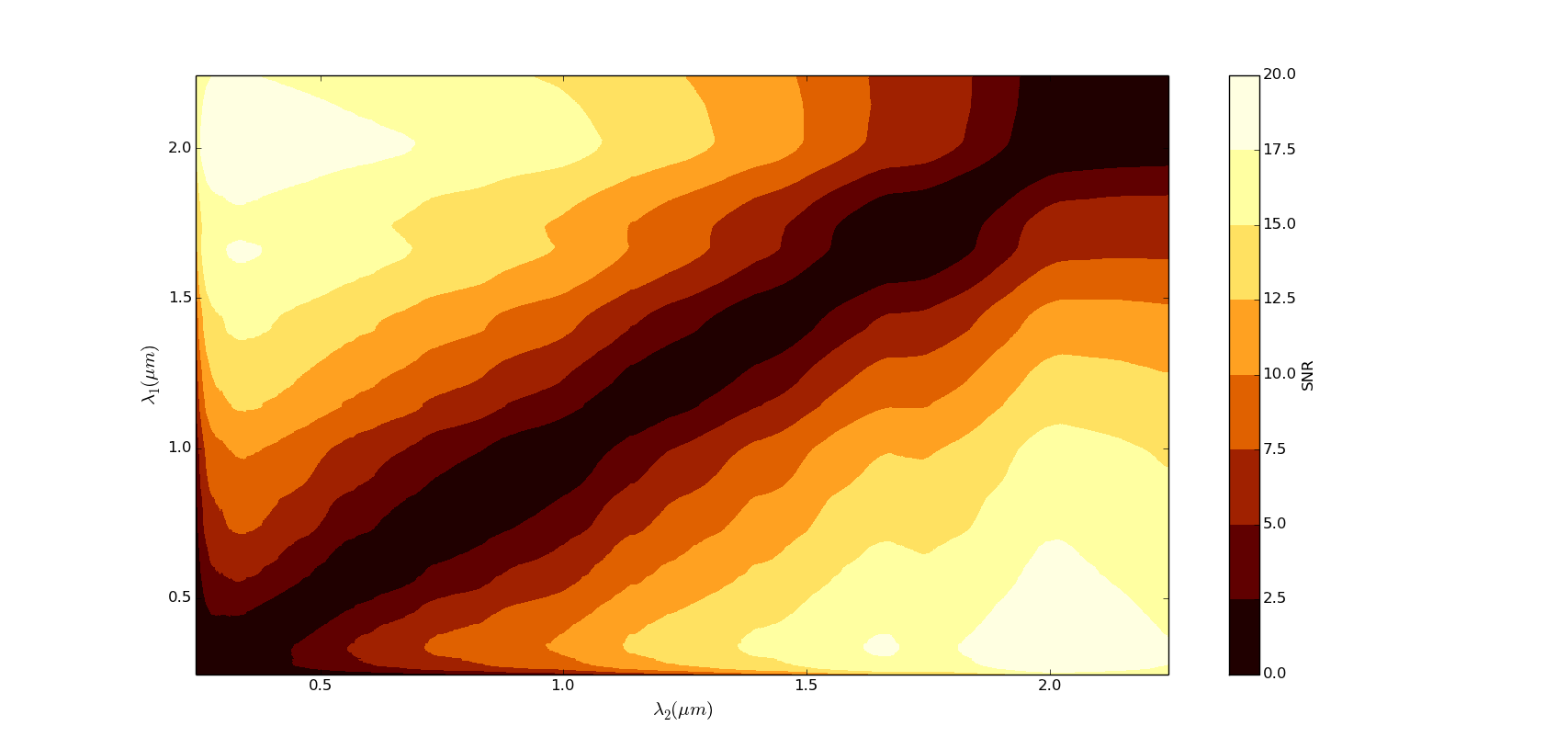
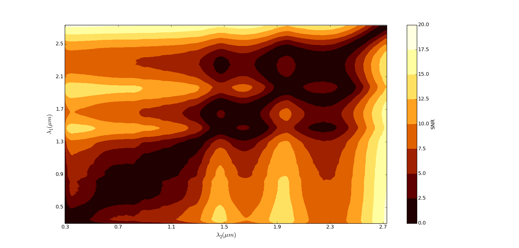
Figure 4.— The spectroastrometric SNR of the Earth-Moon system shown for a combination of wavelengths at R = 1.5 (top) and R = 5 (bottom). Any point on the plots corresponds to a pair of wavelength bands marked on the x and y axes. The color contours indicate the level of SNR achieved when the centroids of those two wavelength bands are compared. We assume a SNR of 5$-\sigma$ or greater would yield a detection. All calculations were done for a model system analogous to our Earth and Moon located 1.34 parsecs away in the habitable zone of $\alpha$ Cen A, with an exposure time lasting 24 hours, and a 12-m telescope diameter.

4.1.2 Earth-like Exomoon Orbiting a Jovian

In a Jovian-Earth system, the Earth-like moon outshines the Jovian in the NIR methane absorption bands, shown in Figure 5. The maximum fraction of the moon’s flux for the Jovian-Earth system occurs at $\lambda$ = 1.83 $\mu$m, contributing 99.1$\%$ to the total flux, although the use of this band in the spectroastrometric signal does not produce the highest SNR due to its higher noise; a higher SNR is achieved in the methane band near 1.4 $\mu$m, albeit at slightly smaller centroid offset.

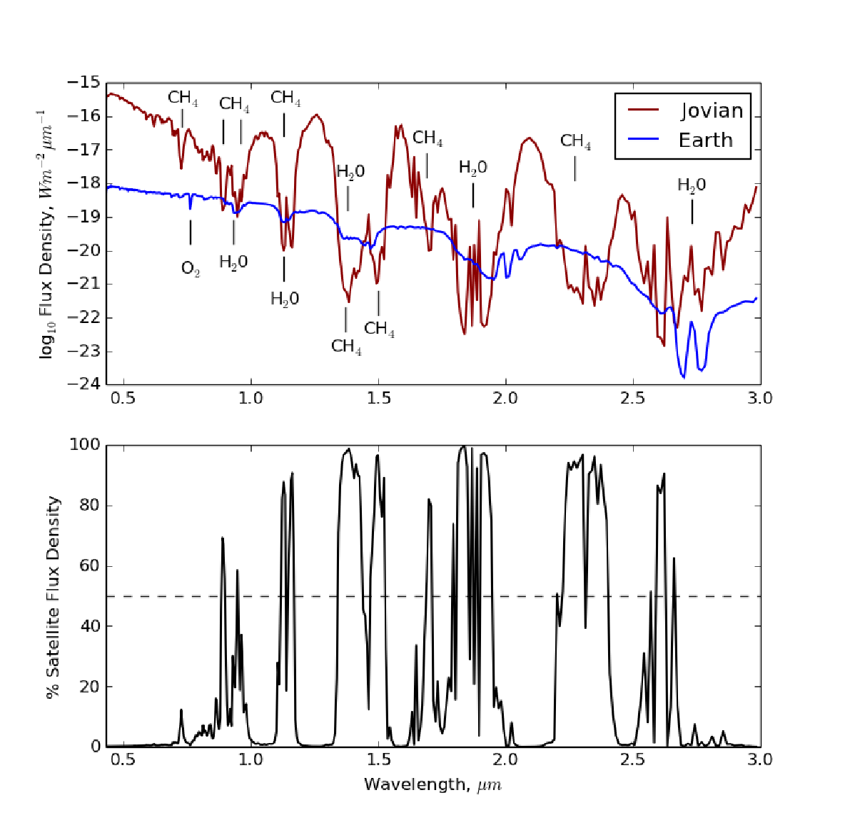
Figure 5.— The flux of the Earth-like moon and the warm Jupiter at quadrature phase angle as a function of wavelength in microns (top) and the contribution of flux due to the moon shown as a fraction of the total flux (bottom). The maximum fraction of the moon’s flux for the Jovian-Earth system occurs at $\lambda$ = 1.83 $\mu$m, contributing 99.1$\%$ to the total flux.

The Jovian-Earth system at 10 pc produces maximum SNRs above 5$-\sigma$ for the parameters in Table 1, assuming spectral resolutions between R = 2 to R = 500, and wavelength pairs drawn from 0.430 - 0.571 $\mu$m and 0.858 - 0.947 $\mu$m. Table 3 lists the optimum wavelength pairs for a selection of spectral resolutions. To illustrate how the SNR changes as a function of spectral resolution, Figure 6 displays the SNR for a range of combinations of wavelengths for two different spectral resolutions. Note that in this model system several wavelength pairs would achieve a SNR well above the detection threshold of 5$-\sigma$, although the optimum resolution will ultimately depend upon the instrument design. Figure 7 shows a slice through this plot with the choice of one wave band centered at 0.89 $\mu$m; this shows that a broad range of comparison wavelengths could be used.

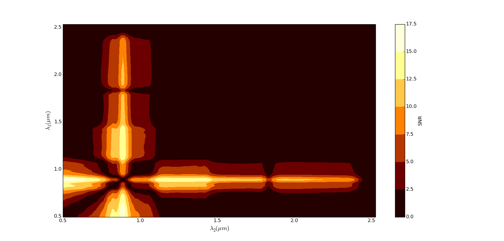
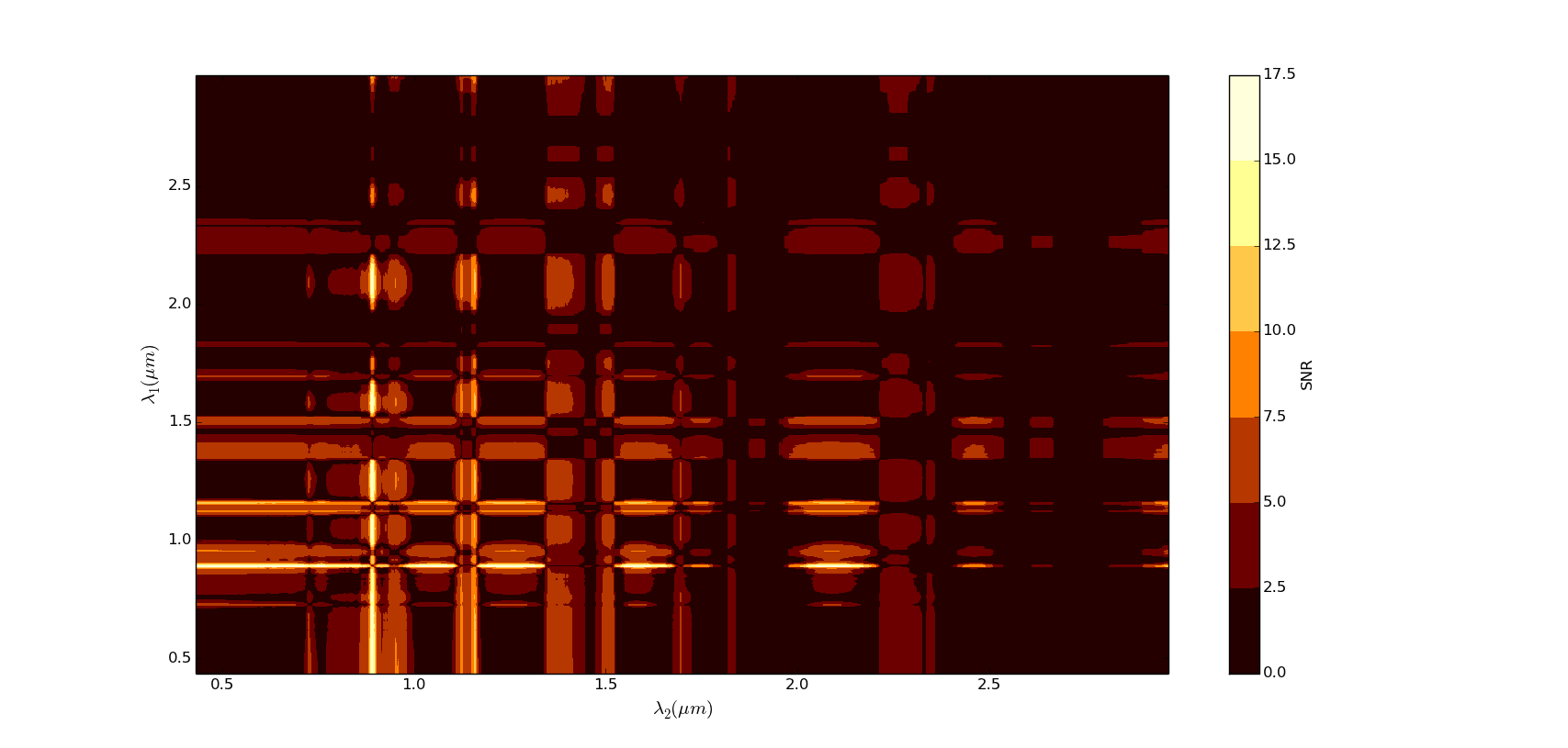
Figure 6.— The spectroastrometric SNR of the Jovian-Earth system shown for a combination of wavelengths at R = 4 (top) and R = 50 (bottom). Any point on the plots corresponds to a pair of wavelength bands marked on the x and y axes. The color contours indicate the level of SNR achieved when the centroids of those two wavelength bands are compared. We assume that a SNR at or above 5$-\sigma$ could yield a detection. All calculations were done for a model Jovian-Earth system located 10 parsecs away, orbiting at 1 AU around a G2V star, with an exposure time lasting 24 hours, and a 12-m telescope diameter.

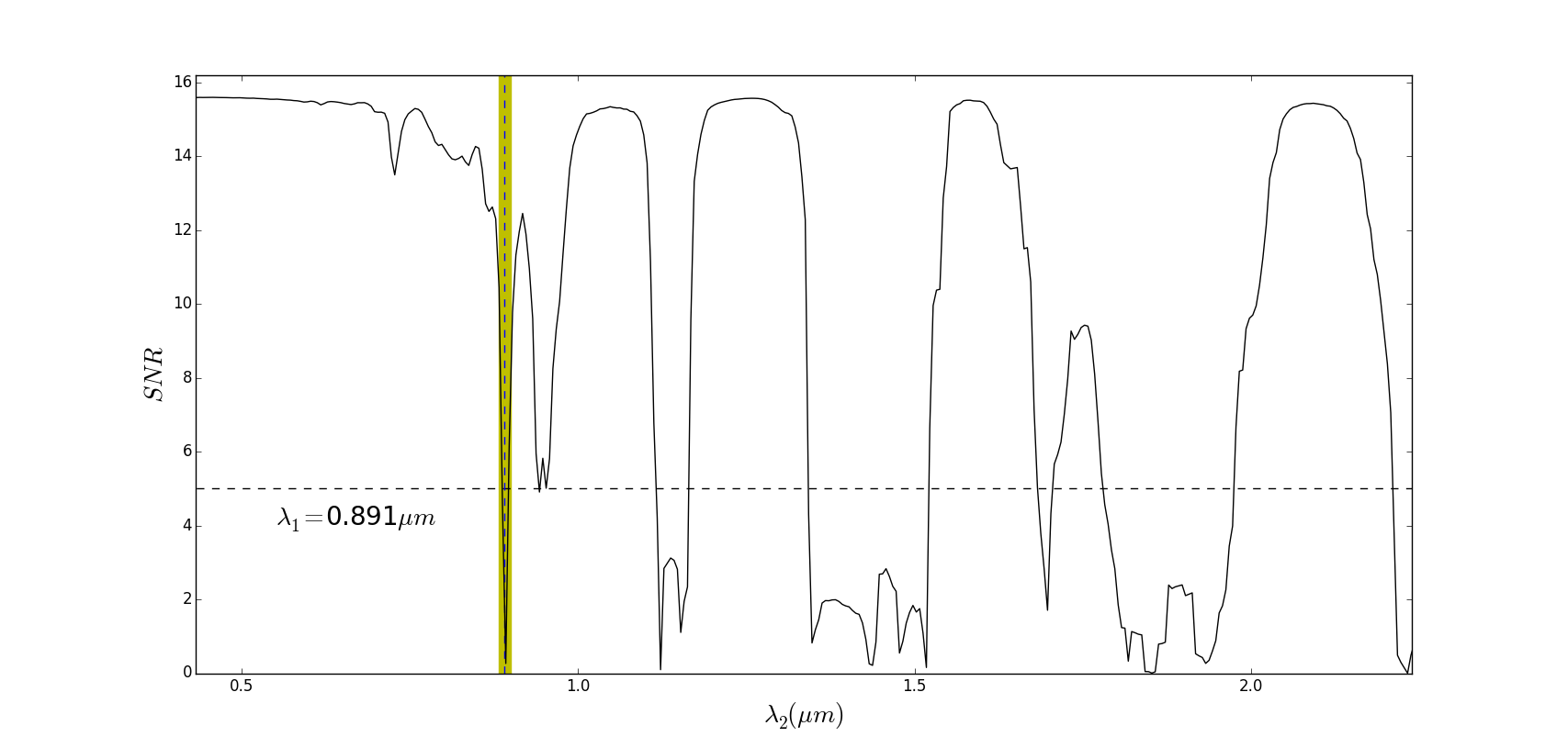
Figure 7.— Methane absorption in the Jovian atmosphere leads to the moon-dominated band with a central wavelength of 0.891 $\mu m$ for R = 50 (marked for reference on figure by blue dashed vertical line and shaded green region). Fixing the centroid from this band as one of our comparisons, the plot shows the SNR (plotted as a black line) for each other band with resolving power R = 50 where signal is measured relative to that fixed 0.891 $\mu m$ band.

4.2. Characterization of an Earth-Moon system around $\alpha$ Cen A

Once a planet-moon system is identified with spectroastrometry, more telescope time will be expended on a habitable-zone system with astrobiological interest in an attempt to characterize the moon-planet system more fully. If spectroastrometric measurements can be made simultaneous to spectroscopic measurements, then the time will concurrently be used for high precision spectroscopy to characterize the atmosphere and look for molecular signatures, as well as to more precisely characterize the spectroastrometric signal.

In particular, the spectroastrometric offset can be used to separate the individual spectra of the planet and moon, to measure the orbit of the moon, and to measure the mass of the planet. As a concrete example, we consider an Earth-Moon twin system observed for a total exposure time of one month. The motion of the moon about the planet will cause the centroid to vary with time. In the case of a circular, face-on system, the angular motion of the centroid can be followed with time to trace out the (nearly) Keplerian orbit of the moon about the planet. Once an orbit is completed, the angular motion can then be removed to give the centroid offset as a function of time; then, as a function of wavelength this can be binned to give the scalar centroid offset.

We ran a Monte Carlo simulation (§3.4) of an Earth-Moon twin orbiting $\alpha$ Cen A, which is the most favorable case for detection and characterization of a moon with spectroastrometry; the proximity of this star favors many modes of exoplanet detection (Eggl et al., 2013). We assume that the planet/moon instellation is the same as Earth’s, which puts the semi-major axis at 1.23 AU; planet orbits can be stable for long timescales at this distance given the right properties (Andrade-Ines & Michtchenko, 2014). We ignore the effect of the companion star ($\alpha$ Cen B) on the observation; however, this may contribute a potential source of noise. Since the effective temperature of the star ($T_{eff}=5790$ K) is slightly hotter than the Sun, we multiply our simulated spectra by the ratio of Planck functions at the two temperatures, divided by the ratio of the temperatures to the fourth power (to maintain the same incident flux).

In Figure 8, we used the Monte Carlo simulations of a 28-day direct imaging observation of the Earth-Moon analog system (orbiting $\alpha$ Cen A) to measure the centroid offset, assuming that the motion is face-on, circular, and that the angular motion can be corrected for. This shows that a SNR can be achieved that varies with wavelength between the extremes of the planet centroid (at zero) and the moon centroid (at 1.9 mas). The detection is highly significant, a total of 169$-\sigma$ (in practice additional sources of noise may reduce this value).

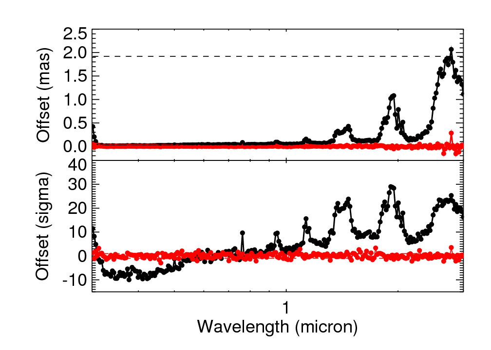
Figure 8.— (Top) Centroid offset, $c(\lambda)$, versus wavelength for a simulated observation of an Earth-Moon twin at 1.34 pc. The orbital motion of the system has been removed (it is assumed to be face-on). The black line is along the axis connecting the Earth and Moon; the red line is perpendicular. The zero point is centered on the Earth. (Bottom) Significance of the centroid offset relative to the mean centroid in the directions parallel (black) and perpendicular (red) to the line connecting the Earth and Moon.

4.2.1 Spectral Distentanglement

We can then use this measurement to approximately separate the spectra of the planet and moon as follows. If we assume that the extremes of the centroid motion with wavelength correspond with the positions of the planet and the moon, then we can identify the two wavelengths at these extremes, $\lambda_{1}$ and $\lambda_{2}$ respectively, and compute the centroid offset signal, $S_{max}=S(\lambda_{1},\lambda_{2})$. We can then divide the centroid offset relative to the planet-dominant wavelength, $S(\lambda,\lambda_{2})$, by the maximum offset, $S_{max}$. Then, since the center of light varies between the planet and the moon, the fraction of flux from the moon is simply

$$f_{moon}=S(\lambda,\lambda_{2})/S_{max},$$ (13)

and the planet is

$$f_{planet}=1-S(\lambda,\lambda_{2})/S_{max}.$$ (14)

We can then multiply this by the total flux, $F_{tot}$, to recover the spectra of the individual bodies, $F_{moon}=f_{moon}F_{tot}$ and $F_{planet}=f_{planet}F_{tot}$. An example of this based on the simulated 28-day observation of the Earth-Moon twin orbiting $\alpha$ Cen A (at $d=$ 1.34 pc) with a 12-meter telescope and 300 wavelength bins from 0.3 to 3 micron ($R=130$) is shown in Figure 9. The recovered spectra of the bodies match the input spectra, and this approach allows ‘cleaning’ the spectrum of the planet from the contribution from the moon. This could enable spectral retrieval to be carried out on the individual bodies, constraining their atmospheric properties and compositions with further modeling.

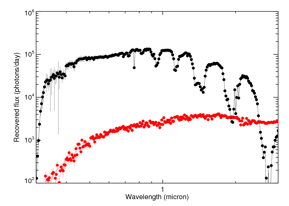
Figure 9.— Recovered spectra of the Earth (black) and Moon (red) using the spectroastrometric offset. The lines show the input spectra; the dots show the recovered spectra.

If it cannot be determined whether the moon-centered wavelength is truly dominated by the moon, then another approach is to estimate the semi-major axis from the mass measured with another technique, such as reflex motion of the star measured with astrometry or radial velocity. Then the predicted semi-major axis can be computed from the period of the spectroastrometric variation, and then this may be used to disentangle the spectra assuming one wavelength is dominated by the planet.

4.2.2 Planet Mass and Orbit Characterization

The time dependence of the spectroastrometric signal can be used to measure the mass of the planet. Based on the simulation of a 28-day signal for a face-on Earth-Moon system at 1.34 pc, we chose the wavelength bins dominated by the Earth and Moon, respectively at 0.35 and 2.75 micron with $R=130$. We then measured the difference between the centroids at these wavelengths with time assuming 1-day exposures; Figure 10 shows a comparison of the input positions, the measured positions, and the best-fit circular orbit (this can be easily extended to an elliptical or edge-on orbit, but we picked this face-on system as an example). We ran 100 realizations of the observations, and we found $M=1.03\pm 0.12M_{\oplus}$ (the measured mass includes the mass of the moon). This relies on having two wavelengths at which the moon and the planet dominate the flux; it may be possible to improve the precision with modeling of the data, which we leave to future investigation.

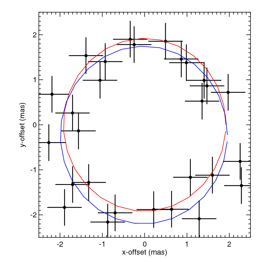
Figure 10.— Simulated spectroastrometric orbit of the Moon-Earth system at 1.34 pc, which is the difference between the $\lambda=2.76$ and $0.35$ micron with $R=130$. The red curve shows the input positions, the crosses show the measured positions at 1-day intervals, while the blue shows the best-fit ellipse for one Monte Carlo realization of the observations.

4.3. Distance and Telescope Size Dependence

The SNR’s simultaneous dependence on distance and telescope diameter for the Jovian-Earth system is shown in Figure 11. Using the wavelength pair $\lambda_{1}$ = 0.45 $\mu$m and $\lambda_{2}$ = 0.89 $\mu$m at R = 50 and $t_{obs}$ = 24 hrs, a 6.7-m telescope would be sufficient to detect an Earth-like moon orbiting a Jovian around a Sun-like star at 10 pc using spectroastrometry with a confidence of 5$-\sigma$. According to the Gliese Catalog of Nearby Stars, there are about 20 main sequence F, G, and K type stars within 10 parsecs that could be used as potential targets. These systems and the diameters needed to detect such a planet-moon system with a confidence of 5$-\sigma$ may be seen in Figure 12. Since the effective temperature of each star differs from the Sun, we multiply our simulated spectra by the ratio of Planck functions at the two temperatures, divided by the ratio of the temperatures to the fourth power (to maintain the same incident flux, which is assumed to be the Solar constant). This assumes that the albedos of the planets remain the same for planets orbiting stars of different spectral types, and that the stellar spectral features differ slightly; both assumptions are approximate, but we expect will have a small effect on our results compared to, for example, planets with different atmospheric compositions that what we have simulated.

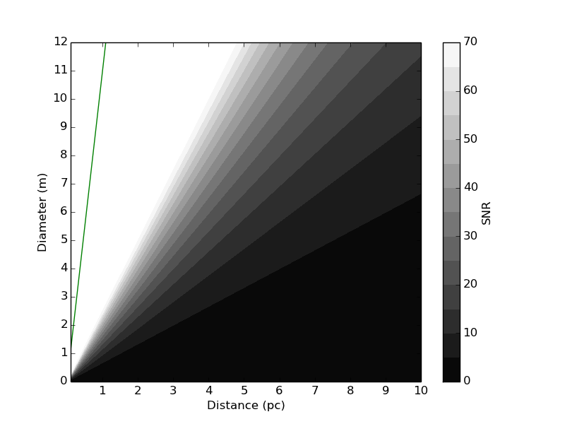
Figure 11.— How the SNR scales with telescope diameter and distance from the observer for the Jovian-Earth system observed between 0.45 $\mu$m and 0.89 $\mu$m at R = 50. The white region shows SNR $\geq$ 70$-\sigma$, and the grayscale shows varying SNR strengths, where the black region shows a non-detection ($<$5$-\sigma$). The green line indicates the telescope diameter needed to directly resolve the Earth-like exomoon from the Jovian planet at 0.89 $\mu$m as a function of distance, in which case spectroastrometry would not be the primary method to detect an exomoon.

The SNR’s dependence on distance from the observer arises from both the signal’s inverse relationship to the distance and the flux’s contribution to the noise, where the total flux $F_{\lambda}$ is inversely proportional to the square of the distance d. Equation 12 shows that the SNR scales as $d^{-2}$, where one power comes from the decreasing angular separation of the moon and planet, and one power comes from the noise caused by decreasing flux of the moon.

The telescope diameter affects the width of the point spread function as $D_{tele}^{-1}$, as well as the total number of photons incident on the detector in a given exposure time $t_{obs}$ as $D_{tele}^{2}$, giving a scaling of the SNR as $D_{tele}^{2}$, as shown in equation 12. Given the overall dependence of SNR as $(D_{tele}/d)^{2}$, the volume which can be surveyed to a fixed SNR scales as $d^{3}\propto D_{tele}^{3}$ (holding other parameters fixed). If the diameter of the telescope is decreased, then the observing time needs to increase as $t_{obs}\propto D_{tele}^{4}$ to obtain an equivalent SNR; thus, either fewer systems can be surveyed due to the longer observing time, or the observing time will increase until systematic errors dominate the noise.

We have focused on habitable-zone planet/moon systems around G stars in this paper, but moons should be searched for around planets at a range of star-planet/moon separations. More distant planet-moon pairs will have lower intensity due to the decreased flux they receive from the star: $F_{\lambda}\propto a^{-2}$, where $a$ is the semi-major axis of the orbit of the planet and moon about the star. However, their Hill spheres will expand due to their larger separation from the star, so if the moon’s orbital distance is a fixed fraction of the Hill sphere, then the spectroastrometric signal will increase $\propto a$ due to the wider moon-planet separation. These two effects compensate to cause an equal SNR as a function of the distance of the planet/moon system from the host star.

5. Discussion

The detection of an exomoon is a long-sought discovery which could profoundly impact our understanding of planet and satellite formation and evolution, including that of our own Solar System. It is clear that moons can outshine their planets at some wavelengths and contribute to apparent variability of a planet (Williams & Knacke, 2004; Moskovitz et al., 2009; Robinson, 2011); in practice, though, it may be difficult to prove that spectroscopic or time-dependent signatures are in fact due to a moon. Since a moon should be spatially separated from a planet, and the separation should follow a (nearly) Keplerian orbit as a function of time, spectroastrometry gives a means of detection that is more definitive, and would allow measurement of the properties of the planet-moon system.

If the separation of the planet and moon is similar to the width of the instrumental point-spread function (PSF), then one can simply resolve the planet and moon. For example, a favorable configuration of a satellite orbiting at 0.25 of the Hill radius of a Jovian-mass planet orbiting at $\approx 1$ AU around a star at 3 pc will have a maximum angular separation of $\approx 6$ mas. This is about the angular resolution at 0.5 $\mu$m of an 8-meter space telescope; in practice, the angular separation will be smaller, so most planet-moon systems will be unresolved, hence the need for spectroastrometry. The $\alpha$ Cen A case of an Earth-Moon analog can almost be resolved directly: at 0.35 $\mu$m, a 12-meter telescope has a resolution of $\approx 2.7$ mas, while the angular separation of the Earth-Moon analog is $1.9$ mas. Since the Moon is much fainter than the Earth at these wavelengths ($\lesssim$ 1%), it may be difficult to deconvolve the light, and thus spectroastrometry will still be favored for detection of the moon.

We have chosen 3 micron as the long-wavelength limit for these observations based on the fact that current coronagraphic designs are considering 2 micron as a possible wavelength cutoff, with a possible extension to 3 - 5 micron (Dalcanton et al., 2015); longer wavelengths have the problem of a larger inner working angle and noise due to thermal emission from the telescope. Spectral coverage that extends to 3 $\mu$m covers the water band at 2.7 $\mu$m and the methane band at 2.3 $\mu$m; these bands have the advantage of being dominated by the moons in the two cases we have considered. In particular, for measuring the mass of the Earth-like planet in the Earth-Moon analog case, the 2.7 $\mu$m band is critical for being able to measure the planet-moon semi-major axis. At 3 $\mu$m we find that there are $\approx 7$ KV stars out to 5 parsecs which can be resolved at $>2\lambda/D_{tele}$ for $D_{tele}=12$ meters; 15 GV stars out to 17 parsecs; and 36 FV stars out to 24 parsecs (we have not considered stars beyond 25 parsecs). The possibility of detection of an exomoon in these systems depends strongly on the potential properties of the exomoon-exoplanet systems present, including their frequency.

Another issue we have not considered is the effect on these observations of exo-zodiacal light due to scattering/thermal emission by dust. This diffuse emission component could have a spectrum similar to that of a moon, and if concentrated in a region near the planet, may be confused with the effect of a moon. If spread throughout the system it would contribute to the noise of the observation, which grows more severe at longer wavelengths due to the larger PSF, which scales in solid angle (or area on the detector) as $\lambda^{2}$. If (exo-) zodiacal light is a significant source of noise, then shorter wavelengths may be favored. We estimate (Agol, 2007) the ratio of the flux of the exozodi flux within the planet’s PSF, $F_{EZ}$, to flux of the host star, $F_{*}$, to be:

$$\frac{F_{EZ}}{F_{*}} = \frac{d^{2}}{r^{2}}\tau_{EZ}S_{fac}\left(\frac{\lambda}{D_{tele}}\right)^{2}$$ (15)

$$= 6\times 10^{-12}d_{pc}^{2}r_{AU}^{-2}\frac{\tau_{EZ}}{10^{-9}}\left(\frac{\lambda}{3\mu{\rm m}}\right)^{2}\left(\frac{D_{tele}}{12{\rm m}}\right)^{-2},$$ (16)

where $\tau_{EZ}$ (units sr^-1) relates the incident stellar flux to the exozodi surface brightness, and $r$ is the planet-star separation. This is less than the Moon flux for Solar-System like exo-zodiacal light, but it can increase with distance, wavelength, or dust surface density, and thus may play a factor for more distant, young systems. Older systems may be largely void of dust (like our Solar System).

The precise choice of the wave bands used for detection will depend on multiple factors rather than just optimizing the signal-to-noise ratio. For example, if a telescope has a short or long-wavelength cutoff that differs from what we assumed, this may require a different choice of band. If a narrow wavelength range is required, then it may be necessary to choose more closely spaced wavelengths than what we have chosen. As an example, consider the fiducial Earth-Moon twin system with parameters from Table 1. We tried all pairs of wavelengths from 0.3 - 3 micron, and resolutions from R=1-10 (in steps of 1) which give SNR $>10$ for this simulated system (for a 12-meter telescope and 1-day observation). From these, we found wave bands that give the largest spectroastrometric signal, $S(\lambda_{1},\lambda_{2})$: we find that $\lambda_{1},\lambda_{2}=0.335,2.73$ micron and R$=10$, gives a centroid offset that is 90% of the Moon-Earth sky separation at quadrature (SNR = 14). Higher resolutions can approach 100% (Fig. 3), but at lower SNR; this is what was required for the characterization of the system (§4.2).

Another consideration is the separation in wavelength: if the instrumental systematic errors of the centroid measurements grow with the separation in wavelength, then it may be advantageous to choose two bands that are closely spaced in wavelength. Amongst the SNR $>10$ band pairs for the Earth-Moon system at 1.34 pc, we find $\lambda_{1},\lambda_{2}=2.3,2.7$ micron (R=10) gives a centroid offset that is 75% of the sky separation. The precise choice of bands and resolutions will depend strongly on the planet properties and stellar distance, as well as the properties of the coronagraphic telescope, so these examples are merely for illustration.

With the detection of a moon with spectroastrometry, there are several applications of the detection which may be used for characterizing the planet-moon system. A spectroastrometric detection will confirm that a spectroscopic moon signal is truly due to an exomoon, and not, for example, due to varying temperature or gas mixing ratio profiles within the planet’s atmosphere; it will also confirm that the planet is in fact a planet. The variation of the spectroastrometric signal with time will follow the orbit of the moon about the planet, giving the period of the moon’s orbit when monitored with time. As shown above (§4.2), using Kepler’s law, the period and semi-major axis allow the determination of the mass of the planet plus moon; this could enable the mass measurement of an Earth-Moon twin at 1.34 pc with a 12-meter telescope at 0.35 and 2.76 micron. This will also potentially allow the determination of the semi-major axis, orbital inclination, and eccentricity of the moon, if the signal-to-noise is sufficient. These applications require that wavelengths can be identified at which the planet and moon each dominate the flux, although this may be difficult to prove in practice as the spectroastrometric signal is degenerate between the moon’s radius, $R_{m}$, and semi-major axis, $a_{mp}$, $S\propto R_{m}^{2}a_{mp}$.

In addition to the spectroastrometric signal, which yields the difference of the center-of-light between the moon and the planet, if the absolute astrometric signal of the planet can be measured, then it might be possible to also measure the mass of the moon due to the reflex motion of the planet about the center of mass with its moon. However, this signal, which is of order the size of the Earth for the Earth-Moon system, may be swamped by the contribution of the Moon’s signal to the centroid, which would need to be removed precisely to measure the offset of the Earth from the center of mass with the Moon; this will require identification of the wavelength at which the Moon-Earth flux ratio is less than the Moon-Earth mass ratio, such as near $0.35$ micron (Fig. 3). In addition, the center-of-mass offset of the planet’s light is in the opposite direction of the of the center-of-light offset (relative to the center of mass) at wavelengths where the moon has a larger flux fraction. There is a wavelength at which the two offsets cancel, at which point the center of light coincides with the center-of-mass; for the Earth-Moon system at quadrature this occurs at 0.493 $\mu$m (Figure 3). The astrometric signal will also be affected by the non-uniform illumination and non-uniform albedo (or thermal emission) of the Earth, which will vary with orbital phase and rotation of the planet, which should be accounted for if the astrometric precision is sufficiently high. This could, in fact, provide another opportunity to detect spatial variations in the surface of the planet, and potentially reveal the full obliquity of the planet, recirculation of heat (which would be affected by the atmospheric pressure and opacity of the planet), and surface markings (or persistent cloud features). In addition, perturbations by other planets in the system can affect the motion of the center-of-mass; for the Earth-Moon system, these perturbations also have an amplitude that is comparable to the radius of the Earth. Despite these complications, this measurement could also be attempted with a coronagraphic telescope capable of precision astrometry of planets, which could be measured with respect to the position of the host star. A diffractive element introduced into a high-contrast imaging coronagraph can yield the astrometric position of the star, and thus allow the precise measurement of the planet’s orbit with respect to the star (Guyon et al., 2013).

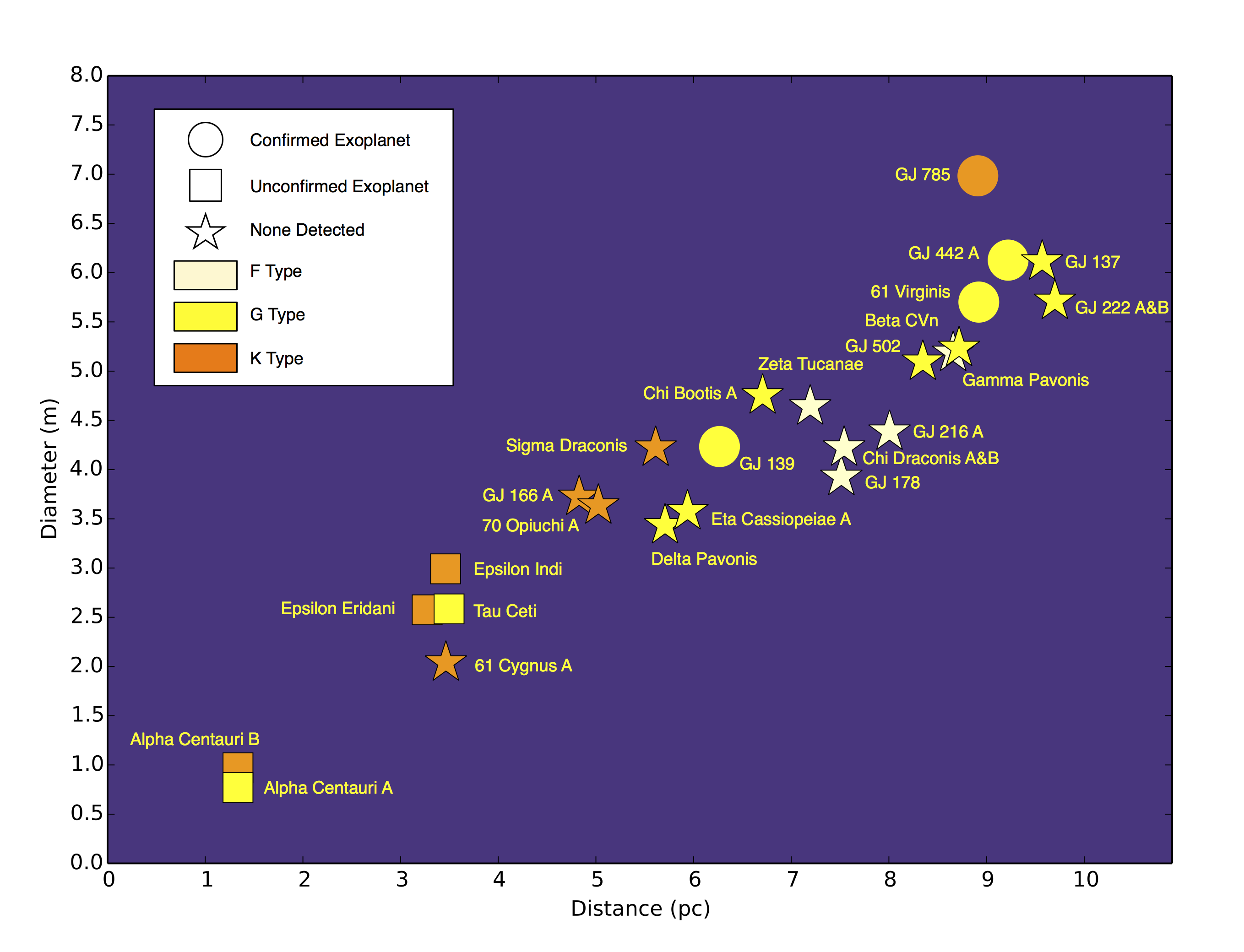
Figure 12.— Minimum telescope diameters needed to obtain a 5$-\sigma$ spectroastrometric detection between 0.45 $\mu m$ and 0.89 $\mu m$ of an Earth-like exomoon orbiting a warm Jupiter in the approximate habitable zones of the systems labeled above, displayed at their respective distances. The different colors represent the spectral types F (pale yellow), G (yellow), and K (orange). The circles represent the systems with confirmed exoplanets, the squares for systems with unconfirmed exoplanets, and the stars for systems in which exoplanets have yet to be detected.

A spectroastrometric detection of an exomoon can potentially result in a detection of eclipses/transits/mutual events. The orbit of the moon about the planet measured from spectroastrometry may allow one to forecast whether and when a moon/planet will transit. Knowing whether the events will occur and observing at the forecast times gives a significant advantage over trying to initially detect an exomoon with eclipses/transits/mutual events for which continuous observations are required and a successful detection depends on the unknown geometry of the orbits (Cabrera & Schneider, 2007). There are four possibilities of the system geometry to consider (Schneider et al., 2015): 1) if the moon’s orbit has a small inclination with respect to the planet’s orbit (which can be measured from its motion about the star with time), then the moon can regularly pass between the star and the planet, causing a shadow to be cast on the planet, which may be visible by a dimming of the planet at the predicted time of the stellar eclipse; 2) the passage of the moon into the planetary shadow (with respect to the star) can also yield a dimming due to the lunar eclipse; 3) if the inclination of the moon relative to our line of sight is nearly edge-on, then one might observe a transit of the planet by the moon, causing a dimming at the predicted time (Livengood et al., 2011); 4) likewise, the moon can pass behind the planet. It is possible for cases 1/2 and 3/4 to occur simultaneously (given a fortuitous geometry), causing an even larger depth. The latter two cases have a $\approx 2$% probability for a randomly placed observer of the Earth-Moon system, which is about four times larger than the probability of viewing the Earth to transit the Sun ($\approx 0.5$%). Any four of these configurations, if detected at sufficient signal-to-noise, might yield a measurement of the radii of the planet and/or the moon (or their ratio), giving a means of determining the density of the planet (and possibly the moon). In addition, if the spectral dependence of the transits/eclipses are measured, this might yield the detection of spatially-resolved features on either body. Heller & Albrecht (2014) have also studied the possibility of measuring the Rossiter-McLaughlin effect in high-resolution spectroscopy of resolved exoplanet being transited by an exomoon; initial spectroastrometric detection could be used to forecast the timing of these events.

Spectroastrometry may also enable a measurement of the spectrum of the moon. In the case of an Earth-like planet orbiting a giant planet in the habitable-zone, this may be one of the best ways to characterize the atmosphere of the planetary companion. Once the solution for the moon-planet orbit is found, the observations can be integrated for a longer time, possibly allowing a spectrum to be built up of both bodies (§4.2). This technique works best if two wave bands can be pinpointed within which the planet dominates in one band and the moon in the other; then the spectroastrometric signal between these two bands gives the sky separation of the bodies at each time. In the example we considered of a face-on circular orbit (§4.2), the planet-moon separation is unchanged with time. For a different orbital configuration, the planet-moon separation needs to be modeled as a function of time and wavelength with a Keplerian orbit. Then the size of the orbit as a function of wavelength (with respect to a reference wavelength) can be used for the spectral decomposition. The edge-on case will have a signal that is reduced by $\approx\sqrt{2}$. This measurement can possibly allow the correction of a planet’s spectrum for contamination by a moon, avoiding a potential false-positive for disequilibrium chemistry (Rein et al., 2014). The recovered spectra of both bodies could constrain their albedos and their thermal emission properties, further constraining the atmospheric properties.

With measurements of the orbital and bulk properties of the moon-planet system, one can potentially place constraints upon the formation of the system, as well as its tidal evolution. In particular, the location of the orbit within its Hill sphere, and the eccentricity of the orbit, will constrain tidal migration and circularization of the system, which can potentially yield a constraint upon tidal evolution theory (Heller et al., 2014).

We end by mentioning some other issues to consider in future work. We have only considered two example planet-moon compositions, and a limited range of an (admittedly) large parameter space. The sizes of the planet and moon, spectral type of the host star, planet-moon separation, spectral variability of the planet and/or moon, semi-major axis of the stellar orbit, exo-zodiacal light, presence of other planets, presence of rings (about the planet or star), inclination of the orbital axes, eccentricities, and more can affect the detection. Most importantly, the composition and presence (or absence) of an atmosphere, albedo, presence of clouds or hazes, and other properties of the atmospheres or reflective surfaces will affect which bands should be observed, and at what wavelengths each body will dominate. Planet and/or moon variability should be considered as well. In the case of the Earth-Moon system, the quadrature Earth varies at the level of roughly ten percent over its rotation period (one day). This would be detectable in total flux, and so the spectrastrometric signal could be averaged over the rotation timescale, assuming that the two bands could be measured at the same time. Longer timescale variability could affect the orbital characterization and spectral disentangling; we leave the issue of variability for future work. Tidal heating of an exomoon could enhance the spectroastrometric signal if the temperature were increased to the point of contributing strongly in the absorbing bands of the planet. Multiple moons (or rings) could affect the interpretation of the spectroastrometric signal; we have assumed a single moon based on the logic that the first detections will be of large moons, and large moons might not exist stably with multiple moon companions. The inclination of the moon with respect to the observer will affect the spectroastrometric signal: an edge-on moon will spend some time at a small projected separation from the planet, and so an observation at the wrong time might miss the spectroastrometric signal. This will require additional observing time to sample the (unknown) phase of the moon sufficiently to be able to capture it at maximum elongation. We have only considered observations at quadrature illumination, while the orbital phase dependence of the spectroastrometric signal may yield additional information about the bodies. Also, in computing the spectroastrometric signal, we have ignored the motion of the moon. This should be adequate if the duration of the observation is much shorter than the orbital period of the moon, but for long exposure times or short moon periods, this could affect our signal-to-noise computations. Once a moon is detected, and its orbital period measured, the orbital motion can be accounted for in modeling the spectroastrometric signal as a function of time.

The design of the detector which would allow spectroastrometric measurements needs to be explored. New detector technologies that allow for the measurement of the position and energy of a photon could potentially yield low-resolution spectroscopic images, and the resulting data cube could be binned in wavelength channels to optimize the detection of a moon, and later to optimize the characterization of the spectra as a function of wavelength. Specifically, Microwave Kinetic Inductance Detectors, or MKIDs, and Superconducting Tunnelling Junctions, STJs, have high quantum efficiency and are being multiplexed into larger arrays (Peacock et al., 1996; Day et al., 2003; Mazin et al., 2012). Another possible approach would be to use an integral field unit spectrograph, such as that used on the Gemini Planet Imager (Macintosh et al., 2006). The wave bands that are used could in principle be selected after the observations are made: the smaller body tends to dominate at wavelengths where the larger body is dimmest, so the wavebands can be selected based on the observed molecular band features that are found after the initial spectrum is measured. Then the centroid offset can be searched for by measuring on-band and off-band. The spectroastrometric precision may be affected by the sampling of the point-spread function as a function of wavelength; this should be studied further to determine what pixel/fiber size is required to obtain astrometric precision at each wavelength that is limited by the width of the PSF and number of photons detected, and not its spatial sampling.

We have limited our exploration to a coronagraphic telescope operating out to 3 $\mu$m. Interferometric approaches might allow spectroastrometry to be extended to longer wavelengths, where additional absorption bands could be used and where the thermal emission from the moon can be significant, such as in the TPF-I/Darwin concept operating from 6 - 20 $\mu$m (Lawson et al., 2008; Cockell et al., 2009). This would have great advantages for characterizing the planet-moon system, but involves the significant technical challenges of formation flying, baseline control, and thermal backgrounds. In principle this detection technique could be applied to ground-based direct imaging as well with future large coronagraphic telescopes; Schneider et al. (2015) have mentioned the possibility of detecting the astrometric wobble of a directly imaged giant planet due to an exomoon companion. The precision may be limited more strongly by control of the optics and atmosphere, but nonetheless could possibly detect large moons in the infrared, and spectroastrometry could potentially be more sensitive than absolute astrometry depending on the instrumental and observational design.

One challenge of coronagraphic spectroastrometry is that precise centroiding requires controlling sources of noise, as well as a stable PSF that can be measured astrometrically over a broad range of wavelengths, requiring stable pointing and control of the PSF shape. These requirements may drive stricter tolerances for the design of a high-contrast imaging telescope than the requirements for spectroscopy. For example, the statistical uncertainty for the 28-day observation of a 1.34-pc Earth-Moon system with a 12-meter telescope is $\approx 3$ $\mu$arcsec, and the typical ratio of the astrometric precision can be as small as 0.01-0.1% of the width of the PSF. Thus, the pointing, the variation of the PSF, the characterization of the PSF, and the effects of other sources of noise need to be limited/controlled/calibrated to a very precise level. The telescope design and detector calibration would need to be capable of reaching this sub-pixel precision in measuring the location of the centroid of the planet-moon PSF as it passes across the detector over time; sub-pixel sensitivity variations, detector latency, charge bleeding, and light loss would all have to be controlled or calibrated to high precision to reach the photon-noise limit that we have assumed for this paper. One mitigating factor is that the spectroastrometric signal changes sign and direction as the moon orbits the planet, and should repeat with time, while any systematic errors will likely have a different time dependence.

6. Conclusions

Spectroastrometric detection presents a scientifically promising, but technically challenging, means of detecting and studying satellites of exoplanets, ‘exomoons.’ We have presented two case studies to illustrate the potential for detection of this effect, and urge that studies of future coronagraphic telescope designs take into account the spectroastrometric signal when designing the technical requirements of telescopes and detectors. Subsequent to detection, the characterization of exomoons with spectroastrometry could lead to measurement of the fundamental properties of exoplanet-moon systems, including the mass of the host planet, and could help in pinpointing targets that are valuable for studies of habitability.

We end by making some general recommendations for guiding design of future coronagraphic space telescopes with spectroastrometry in mind: 1) the instrument suite should include the capability of making astrometric measurements as a function of wavelength for a range of spectral resolutions; 2) the pointing control, PSF wing suppression, and PSF stability and calibration should be designed with the capability of making photon-limited astrometric measurements over a broad range of wavelengths; and 3) the instrument wavelength should be extended out to $\approx 3$ micron to cover the water absorption band at which the Moon dominates over the Earth ($\approx 2.7$ micron) and methane band at which the Earth dominates over Jupiter ($\approx 2.3$ micron).

References

- Agol (2007) Agol, E., 2007, MNRAS, 374, 1271
- Agnor & Asphaug (2004) Agnor, C., & Asphaug, E. 2004, ApJ, 613, L157
- Agnor & Hamilton (2006) Agnor, C. B., & Hamilton, D. P. 2006, Nature, 441, 192
- Andrade-Ines & Michtchenko (2014) Andrade-Ines, E. & Michtchenko, T. A., 2014, MNRAS, 444, 2167
- Armstrong et al. (2014) Armstrong, J., Barnes, R., Domagal-Goldman, S., Breiner, J., Quinn, T.R. & Meadows, V.S., 2014, Astrobiology, 14, 277
- Aumann et al. (2003) Aumann, H. H., et al. 2003, IEEE Transactions on Geoscience and Remote Sensing, 41, 253
- Bailey (1998) Bailey, J. A., 1998, SPIE, 3355, 932
- Barnes & O’Brien (2002) Barnes, J. W., & O’Brien, D. P. 2002, ApJ, 575, 1087
- Beer et al. (2001) Beer, R., Glavich, T. A., & Rider, D. M. 2001, Appl. Opt., 40, 2356
- Buratti et al. (2011) Buratti, B. J., Hicks, M. D., Nettles, J., Staid, M., Pieters, C. M., Sunshine, J., Boardman, J., & Stone, T. C. 2011, Journal of Geophysical Research (Planets), 116, E00G03
- Burrows & Sharp (1999) Burrows, A., & Sharp, C. M. 1999, ApJ, 512, 843
- Burrows et al. (2004) Burrows, A., Sudarsky, D., & Hubeny, I. 2004, ApJ, 609, 407
- Cabrera & Schneider (2007) Cabrera, J., & Schneider, J. 2007, A&A, 464, 1133
- Cameron & Ward (1976) Cameron, A. G. W., & Ward, W. R. 1976, Lunar and Planetary Science Conference, 7, 120
- Canup & Ward (2002) Canup, R. M., & Ward, W. R. 2002, AJ, 124, 3404
- Cash (2006) Cash, W., 2006, Nature, 442, 51
- Cockell et al. (2009) Cockell, C.S., et al., 2009, Astrobiology, 9, 1
- Schneider et al. (2015) Schneider, J., Lainey, V. & Cabrera, J., 2015, International Journal of Astrobiology, 14, 191
- Chandrasekhar (1960) Chandrasekhar, S. 1960, Radiative Transfer (Dover)
- Crisp (1997) Crisp, D. 1997, Geophys. Res. Lett., 24, 571
- Dalcanton et al. (2015) Dalcanton, J., Seager, S., Aigrain, S., Battel, S., Brandt, N., Conroy, C., Feinberg, L., Gezari, S., Guyon, O., Harris, W., Hirata, C., Mather, J., Postman, M., Redding, D., Schiminovich, D., Stahl, H.P. & Tumlinson, J., 2015, arXiv:1507.04779, http://www.hdstvision.org
- Day et al. (2003) Day, P.K., LeDuc, H.G., Mazin, B.A., Vayonakis, A., Zmuidzinas, J., 2003, Nature, 425, 817
- Duncan & Kipping (2013) Forgan, D. & Kipping, D., 2013, Monthly Notices of the Royal Astronomical Society, 432, 2994
- Eggl et al. (2013) Eggl, S., Haghighipour, N. & Pilat-Lohinger, E., 2013, ApJ, 764, 130
- Górski et al. (2005) Górski, K. M., Hivon, E., Banday, A. J., Wandelt, B. D., Hansen, F. K., Reinecke, M., & Bartelmann, M. 2005, ApJ, 622, 759
- Guyon et al. (2006) Guyon, O., Pluzhnik, E. A., Kuchner, M. J., Collins, B., & Ridgway, S. T., 2006, ApJS, 167, 81
- Guyon et al. (2013) Guyon, O. et al., 2013, ApJ, 767, 11
- Macintosh et al. (2006) Macintosh, et al., 2006, SPIE, 6272, 62720
- Hall et al. (1995) Hall, D. K., Riggs, G., & Salomonson, V. V. 1995, Remote Sensing of Environment, 54, 127
- Hartmann & Davis (1975) Hartmann, W. K., & Davis, D. R. 1975, Icarus, 24, 504
- Heller (2012) Heller, R. 2012, A&A, 545, LL8
- Heller & Barnes (2013) Heller, R., & Barnes, R. 2013, Astrobiology, 13, 18
- Heller (2014) Heller, R., 2014, ApJ, 787, 14
- Heller et al. (2014) Heller, R., Williams, D., Kipping, D., Limbach, M. A., Turner, E., Greenberg, R., Sasaki, T., Bolmont, É, Grasset, O., Lewis, K., Barnes, R. & Zulaga, J. I., 2014, Astrobiology, 14, 798
- Heller & Armstrong (2014) Heller, R. & Armstrong, J., 2014, Astrobiology, 14, 50
- Heller & Albrecht (2014) Heller, R. & Albrecht, S., 2014, ApJ, 796, L1
- Heller & Barnes (2015) Heller, R., & Barnes, R. 2015, International Journal of Astrobiology, 14, 335
- Heller & Pudritz (2015a) Heller, R. & Pudritz, R., 2015, Astronomy & Astrophysics, 578, A19
- Heller & Pudritz (2015b) Heller, R. & Pudritz, R., 2015, ApJ, 806, 181
- Hinkel & Kane (2013) Hinkel, N. R. & Kane, S. R., 2013, The Astrophysical Journal, 774, 27
- Kaltenegger (2000) Kaltenegger, L. 2000, Exploration and Utilisation of the Moon, 462, 199
- Kaltenegger (2010) Kaltenegger, L. 2010, The Astrophysical Journal, 712, 125
- Kipping (2009) Kipping, D. M. 2009, MNRAS, 392, 181
- Kipping (2011) Kipping, D. M. 2011, MNRAS, 416, 689
- Kipping et al. (2012) Kipping, D. M., Bakos, G. Á., Buchhave, L., Nesvorný, D., & Schmitt, A. 2012, ApJ, 750, 115
- Kouveliotou et al. (2014) Kouveliotou, C., Agol, E., Batalha, N., et al. 2014, arXiv:1401.3741
- Lane & Irvine (1973) Lane, A. P., & Irvine, W. M. 1973, AJ, 78, 267
- Laskar et al. (1993) Laskar, J., Joutel, F., & Robutel, P. 1993, Nature, 361, 615
- Lawson et al. (2008) Lawson, J.R., et al., 2008, SPIE, 7013, 70132N
- Lissauer et al. (2012) Lissauer, J.J., Barnes, J.W. & Chambers, J.E., 2012, Icarus, 217, 77
- Livengood et al. (2011) Livengood, T. A., et al. 2011, Astrobiology, 11, 907
- Lunine & Stevenson (1982) Lunine, J. I., & Stevenson, D. J. 1982, Icarus, 52, 14
- Mazin et al. (2012) Mazin, B., Bumble, B., Meeker, S.R., O’Brien, K., McHugh, S., Langman, E., 2012, Optics Express, 20, 1503
- McCord (1966) McCord, T. B. 1966, AJ, 71, 585
- McKinnon (1984) McKinnon, W. B. 1984, Nature, 311, 355
- Meadows & Crisp (1996) Meadows, V. S., & Crisp, D. 1996, J. Geophys. Res., 101, 4595
- Moskovitz et al. (2009) Moskovitz, N. A., Gaidos, E., & Williams, D. M. 2009, Astrobiology, 9, 269
- Mosqueira & Estrada (2003) Mosqueira, I., & Estrada, P. R. 2003, Icarus, 163, 198
- Muinonen et al. (1989) Muinonen, K., Lumme, K., Peltoniemi, J., & Irvine, W. M. 1989, Appl. Opt., 28, 3051
- Ogihara & Ida (2012) Ogihara, M., & Ida, S. 2012, ApJ, 753, 60
- Peacock et al. (1996) Peacock, A., Verhoeve, P., Rando, N., van Dordrecht, A., Taylor, B.G., Erd, C., Perryman, M.A.C., Venn, R., Howlett, J., Goldie, D.J., Lumley, J. & Wallis, M., 1996, Nature, 381, 135
- Peters & Turner (2013) Peters, M. A., & Turner, E. L. 2013, ApJ, 769, 98
- Peters et al. (2007) Peters, W., et al. 2007, Proceedings of the National Academy of Science, 1041, 18925
- Rein et al. (2014) Rein, H., Fujii, Y., & Spiegel, D. S. 2014, Proceedings of the National Academy of Science, 111, 6871
- Reynolds et al. (1987) Reynolds, R.T., McKay, C.P. & Kasting, J.F., 1987, Advances in Space Research, 7, 125
- Riggs et al. (1999) Riggs, G., Hall, D. K., & Ackerman, S. A. 1999, Remote Sensing of Environment, 68, 152
- Robinson (2011) Robinson, T. D. 2011, ApJ, 741, 51
- Robinson et al. (2010) Robinson, T. D., Meadows, V. S., & Crisp, D. 2010, ApJ, 721, L67
- Robinson et al. (2011) Robinson, T. D., et al. 2011, Astrobiology, 11, 393
- Robinson et al. (2014) Robinson, T. D., Ennico, K., Meadows, V. S., et al. 2014, ApJ, 787, 171
- Sartoretti & Schneider (1999) Sartoretti, P., & Schneider, J. 1999, A&AS, 134, 553
- Salomonson et al. (1989) Salomonson, V. V., Barnes, W. L., Maymon, P. W., Montgomery, H. E., & Ostrow, H. 1989, IEEE Transactions on Geoscience and Remote Sensing, 27, 145
- Sasaki et al. (2010) Sasaki, T., Stewart, G.R. & Ida, S., 2010, ApJ, 714, 1052
- Scharf (2006) Scharf, C. A. 2006, ApJ, 648, 1196
- Simon et al. (2007) Simon, A., Szatmáry, K., & Szabó, G. M. 2007, A&A, 470, 727
- Spergel et al. (2015) Spergel, D., et al., 2015, arXiv:1503.03757
- Stapelfeldt et al. (2014) Stapelfeldt, K.R., et al., 2014, Proc. SPIE 9143, 91432K
- Stark et al. (2015) Stark, C. C., et al., 2015, arXiv:1506.01723
- Sudarsky et al. (2003) Sudarsky, D., Burrows, A., & Hubeny, I. 2003, ApJ, 588, 1121
- Szabó et al. (2006) Szabó, G. M., Szatmáry, K., Divéki, Z., & Simon, A. 2006, A&A, 450, 395
- Tusnski & Valio (2011) Tusnski, L. R. M., & Valio, A. 2011, ApJ, 743, 97
- Waters et al. (2006) Waters, J. W., et al. 2006, IEEE Transactions on Geoscience and Remote Sensing, 44, 1075
- Ward et al. (2002) Ward, W. R., Agnor, C. B., & Canup, R. M. 2002, Lunar and Planetary Science Conference, 33, 2017
- Whelan & Garcia (2008) Whelan, E., & Garcia, P. 2008, Jets from Young Stars II, 742, 123
- Williams & Knacke (2004) Williams, D. M., & Knacke, R. F. 2004, Astrobiology, 4, 400
- Williams et al. (1997) Williams, D. M., Kasting, J. F., & Wade, R. A. 1997, Nature, 385, 234