Geometric Monodromy around the Tropical Limit

Geometric Monodromy around the Tropical Limit

Yuto YAMAMOTO

Y. Yamamoto

Graduate School of Mathematical Sciences, The University of Tokyo,
3-8-1 Komaba, Meguro, Tokyo, 153-8914, Japan yuto@ms.u-tokyo.ac.jp

Received September 02, 2015, in final form June 17, 2016; Published online June 24, 2016

Let $\{V_{q}\}_{q}$ be a complex one-parameter family of smooth hypersurfaces in a toric variety. In this paper, we give a concrete description of the monodromy transformation of $\{V_{q}\}_{q}$ around $q=\infty$ in terms of tropical geometry. The main tool is the tropical localization introduced by Mikhalkin.

tropical geometry; monodromy

14T05; 14D05

1 Introduction

Let $K:={\mathbb{C}}\{t\}$ be the convergent Laurent series field, equipped with the standard non-archimedean valuation,

$$\operatorname{val}\colon\ K\longrightarrow{\mathbb{Z}}\cup\{-\infty\},\qquad k=\sum_{j\in{\mathbb{Z}}}c_{j}t^{j}\mapsto-\min\{j\in{\mathbb{Z}}\,|\,c_{j}\neq 0\}.$$ (1.1)

Let $n\in{\mathbb{N}}$ be a natural number and $M$ be a free ${\mathbb{Z}}$-module of rank $n+1$. We write $M_{\mathbb{R}}:=M\otimes_{\mathbb{Z}}{\mathbb{R}}$. Let further $\Delta\subset M_{\mathbb{R}}$ be a convex lattice polytope, i.e., the convex hull of a finite subset of $M$. We set $A:=\Delta\cap M$. Let $F=\sum\limits_{m\in A}k_{m}x^{m}\in K\big{[}x^{\pm}_{1},\dots,x^{\pm}_{n+1}\big{]}$ be a Laurent polynomial over $K$ in $n+1$ variables such that $k_{m}\neq 0$ for all $m\in A$. We fix a sufficiently large $R\in{\mathbb{R}}^{>0}$ such that $1/R$ is smaller than the radius of convergence of $k_{m}$ for all $m\in A$, and set $S_{R}^{1}:=\{z\in{\mathbb{C}}\,|\,|z|=R\}$. For $q\in S_{R}^{1}$, let $f_{q}\in{\mathbb{C}}[x^{\pm}_{1},\dots,x^{\pm}_{n+1}]$ denote the polynomial obtained by substituting $1/q$ to $t$ in $F$. Let ${\mathcal{F}}$ be the normal fan to $\Delta$ and ${\mathcal{F}}^{\prime}$ be a unimodular subdivision of ${\mathcal{F}}$. Let $X_{{\mathcal{F}}^{\prime}}({\mathbb{C}})$ denote the toric manifold over ${\mathbb{C}}$ associated with ${\mathcal{F}}^{\prime}$. For each $q\in S_{R}^{1}$, we define $V_{q}\subset X_{{\mathcal{F}}^{\prime}}({\mathbb{C}})$ as the hypersurface defined by $f_{q}$ in $X_{{\mathcal{F}}^{\prime}}({\mathbb{C}})$. In this paper, we discuss the monodromy transformation of $\{V_{q}\}_{q\in S_{R}^{1}}$ around $q=\infty$. The limit $q\to\infty$ is called the tropical limit in this paper. The motivation to address this problem comes from the calculation of monodromies of period maps.

Let $\operatorname{trop}(F)\colon{\mathbb{R}}^{n+1}\to{\mathbb{R}}$ be the tropicalization of $F$ defined by

$$\operatorname{trop}(F)(X_{1},\dots,X_{n+1}):=\max_{m\in A}\big{\{}{\operatorname{val}}(k_{m})+m_{1}X_{1}+\cdots+m_{n+1}X_{n+1}\big{\}}.$$ (1.2)

The non-differentiable locus of $\operatorname{trop}(F)$ is called the tropical hypersurface defined by $\operatorname{trop}(F)$ and denoted by $V(\operatorname{trop}(F))$. The tropical hypersurface $V(\operatorname{trop}(F))$ is a rational polyhedral complex of dimension $n$. The main theorem of this paper is Theorem 4.5, which gives a concrete description of the monodromy transformation of $\{V_{q}\}_{q\in S_{R}^{1}}$ in terms of the tropical hypersurface $V(\operatorname{trop}(F))$ in the case where $V(\operatorname{trop}(F))$ is smooth (see Definition 2.7). The monodromy of $\{V_{q}\}_{q\in S_{R}^{1}}$ is also discussed in [2, Appendix B.2] and Theorem 4.5 is covered by [2, Proposition B.17]. However, this paper aims to make the relation of the monodromy of $\{V_{q}\}_{q\in S_{R}^{1}}$ to tropical geometry clear. We give a self-contained proof and explicit examples.

When $\Delta$ is smooth and reflexive and the polynomial $F$ gives a central subdivision of $\Delta$, Zharkov [10] also gave a concrete description of the monodromy transformation of $\{V_{q}\}_{q\in S_{R}^{1}}$. The idea of his description is the same as that of ours. By treating his construction systematically, we generalize his result to the case where $\Delta$ is any polytope and the subdivision of $\Delta$ given by $F$ is not necessarily central.

Since the claim of Theorem 4.5 is technical and it is necessary to make preparations in order to state it, we do not state it here and discuss its corollary in the following. Assume $n=1$. Let $\{\rho_{i}\}_{i\in\{1,\dots,d\}}$ be the set of all bounded edges of $V(\operatorname{trop}(F))$. For each $\rho_{i}$, let $\nu_{i1},\nu_{i2}\in{\mathbb{R}}^{n+1}$ be the endpoints of $\rho_{i}$. Let further $V\in{\mathbb{Z}}^{n+1}$ be the primitive vector such that $\nu_{i1}-\nu_{i2}=lV$ for some $l\in{\mathbb{R}}^{>0}$. We define the length $L(\rho_{i})$ of $\rho_{i}$ as $l\in{\mathbb{R}}^{>0}$. Assume that the tropical hypersurface $V(\operatorname{trop}(F))$ is smooth, in the sense that for any vertex $\nu$ of $V(\operatorname{trop}(F))$, there exists a ${\mathbb{Z}}$-affine transformation $\big{(}(m_{ij})_{1\leq i,j\leq 2},(r_{i})_{i=1,2}\big{)}\in{\rm GL}_{2}({\mathbb{Z}})\ltimes{\mathbb{R}}^{2}$ such that in the coordinate $(Y_{1},Y_{2})$ on ${\mathbb{R}}^{2}$ defined by

$$Y_{1}=m_{11}X_{1}+m_{12}X_{2}+r_{1},\qquad Y_{2}=m_{21}X_{1}+m_{22}X_{2}+r_{2},$$

the tropical hypersurface $V(\operatorname{trop}(F))$ coincides locally with the tropical hyperplane defined by $\max\{0,Y_{1},Y_{2}\}$ around $\nu$. Then we have $\nu_{i1},\nu_{i2}\in{\mathbb{Z}}^{n+1}$. The amoeba of $V_{q}$ converges to the tropical hypersurface $V(\operatorname{trop}(F))$ as $q\to\infty$ in the Hausdorff metric [8, 9] and the hypersurface $V_{q}$ is obtained by ‘thickening’ the amoeba of $V_{q}$. Let $C_{i}$ $(i=1,\dots,d)$ be the simple closed curve in $V_{q=R}$ turning around $\rho_{i}$ (see Fig. 1 for an example). Let further $T_{i}\colon V_{R}\to V_{R}$ be the Dehn twist along $C_{i}$.

Corollary 1.1.

If $n=1$ and $V(\operatorname{trop}(F))$ is smooth, then the monodromy transformation of $\{V_{q}\}_{q\in S_{R}^{1}}$ around $q=\infty$ is given by $T_{1}^{L(\rho_{1})}\circ\cdots\circ T_{d}^{L(\rho_{d})}$.

Corollary 1.1 is conjectured by Iwao [4]. Let us illustrate this claim with a simple example. Consider the polynomial $F$ given by

$$F(x_{1},x_{2})=x_{2}^{2}+x_{2}\big{(}x_{1}^{3}+t^{-2}x_{1}^{2}+t^{-2}x_{1}+t^{-1}\big{)}+1.$$ (1.3)

Then we have

$$f_{q}(x_{1},x_{2})=x_{2}^{2}+x_{2}\big{(}x_{1}^{3}+q^{2}x_{1}^{2}+q^{2}x_{1}+q^{1}\big{)}+1,$$

$$\operatorname{trop}(F)(X_{1},X_{2})=\max\{2X_{2},3X_{1}+X_{2},2X_{1}+X_{2}+2,X_{1}+X_{2}+2,X_{2}+1,0\}.$$

The tropical hypersurface $V(\operatorname{trop}(F))$ and the hypersurface $V_{q}$ in this case are shown in Fig. 1. Let $\rho_{i}$ and $C_{i}$ $(i=1,\dots,7)$ denote edges of $V(\operatorname{trop}(F))$ and simple closed curves in $V_{q}$ as shown in Fig. 1. Then the edges $\rho_{1},\dots,\rho_{7}$ correspond to the simple closed curves $C_{1},\dots,C_{7}$, respectively. By simple calculations, we have

$$L(\rho_{1})=2,\qquad\!L(\rho_{2})=4,\qquad\!L(\rho_{3})=12,\qquad\!L(\rho_{4})=L(\rho_{5})=1,\qquad\!L(\rho_{6})=L(\rho_{7})=2.$$

It follows from Corollary 1.1 that the monodromy transformation of $\{V_{q}\}_{q\in S_{R}^{1}}$ is given by $T_{1}^{2}\circ T_{2}^{4}\circ T_{3}^{12}\circ T_{4}\circ T_{5}\circ T_{6}^{2}\circ T_{7}^{2}$.

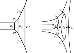
Figure 1: The tropical hypersurface $V(\operatorname{trop}(F))$ and the hypersurface $V_{q}$ for (1.3).

The organization of this paper is as follows: First, we set up the notation in Section 2. In Section 3, we recall the notion of the tropical localization introduced by Mikhalkin [8]. This is the main tool to construct the monodromy transformation of $\{V_{q}\}_{q\in S_{R}^{1}}$. In Section 4, we give an explicit description of the monodromy transformations in any dimension. In Section 5, we show that Corollary 1.1 follows from Theorem 4.5. In Section 6, we give examples in dimension $1$ and $2$. In Section 7, we discuss the relation between Zharkov’s description and ours. This section may also be useful for understanding this paper and a possible first step for getting our idea.

2 Preliminaries

2.1 Tropical toric varieties

Let $M$ be a free ${\mathbb{Z}}$-module of rank $n+1$ and $N:=\operatorname{Hom}_{\mathbb{Z}}(M,{\mathbb{Z}})$ be the dual lattice of $M$. We set $M_{\mathbb{R}}:=M\otimes_{\mathbb{Z}}{\mathbb{R}}$ and $N_{\mathbb{R}}:=N\otimes_{\mathbb{Z}}{\mathbb{R}}=\operatorname{Hom}_{\mathbb{Z}}(M,{\mathbb{R}})$. We have a canonical ${\mathbb{R}}$-bilinear pairing

$$\langle-,-\rangle\colon\ M_{\mathbb{R}}\times N_{\mathbb{R}}\to{\mathbb{R}}.$$

Let ${\mathcal{F}}$ be a fan in $N_{\mathbb{R}}$. We write the toric variety associated with ${\mathcal{F}}$ over ${\mathbb{C}}$ as $X_{\mathcal{F}}({\mathbb{C}})$. For each cone $\sigma\in{\mathcal{F}}$, we set

$$\sigma^{\vee}:=\{m\in M_{\mathbb{R}}\,|\,\langle m,n\rangle\geq 0\mathrm{\ for\ all\ }n\in\sigma\},$$

$$\sigma^{\perp}:=\{m\in M_{\mathbb{R}}\,|\,\langle m,n\rangle=0\mathrm{\ for\ all\ }n\in\sigma\}.$$

Let $U_{\sigma}({\mathbb{C}}):=\operatorname{Hom}(\sigma^{\vee}\cap M,{\mathbb{C}})$ denote the affine toric variety and $O_{\sigma}({\mathbb{C}}):=\operatorname{Hom}(\sigma^{\perp}\cap M,{\mathbb{C}}^{\ast})$ denote the torus orbit corresponding to $\sigma$. We write the closure of $O_{\sigma}({\mathbb{C}})$ in $X_{\mathcal{F}}({\mathbb{C}})$ as $X_{{\mathcal{F}},\sigma}({\mathbb{C}})$.

Let ${\mathbb{T}}:={\mathbb{R}}\cup\{-\infty\}$ be the tropical semi-ring, equipped with the following arithmetic operations for any $a,b\in{\mathbb{T}}$;

$$a\oplus b:=\max\{a,b\},\qquad a\odot b:=a+b.$$

We can also define the toric variety over ${\mathbb{T}}$ as follows. For each cone $\sigma\in{\mathcal{F}}$, we define $U_{\sigma}({\mathbb{T}})$ as the set of monoid homomorphisms $\sigma^{\vee}\cap M\to({\mathbb{T}},\odot)$,

$$U_{\sigma}({\mathbb{T}}):=\operatorname{Hom}\big{(}\sigma^{\vee}\cap M,{\mathbb{T}}\big{)}$$

with the compact open topology. For cones $\sigma,\tau\in{\mathcal{F}}$ such that $\sigma\prec\tau$, we have a natural immersion,

$$U_{\sigma}({\mathbb{T}})\to U_{\tau}({\mathbb{T}}),\qquad\big{(}v\colon\sigma^{\vee}\cap M\to{\mathbb{T}}\big{)}\mapsto\big{(}\tau^{\vee}\cap M\subset\sigma^{\vee}\cap M\xrightarrow{v}{\mathbb{T}}\big{)},$$

where $\sigma\prec\tau$ means that $\sigma$ is a face of $\tau$. By gluing $\{U_{\sigma}({\mathbb{T}})\}_{\sigma\in{\mathcal{F}}}$ with each other, we have the tropical toric variety $X_{\mathcal{F}}({\mathbb{T}})$ associated with ${\mathcal{F}}$,

$$X_{\mathcal{F}}({\mathbb{T}}):=\bigg{(}\coprod_{\sigma\in{\mathcal{F}}}U_{\sigma}({\mathbb{T}})\bigg{)}\bigg{/}{\sim}.$$

Tropical toric varieties are first introduced by Kajiwara [5], see [5] or [6] for details. For a projective toric variety, the associated tropical toric variety is homeomorphic to the moment polytope of it [6, Remark 1.3].

Example 2.1.

The tropical projective space of $n$-dimension is homeomorphic to the $n$-dimensional simplex.

We define the torus orbit $O_{\sigma}({\mathbb{T}})$ over ${\mathbb{T}}$ corresponding to $\sigma$ by

$$O_{\sigma}({\mathbb{T}}):=\operatorname{Hom}\big{(}\sigma^{\perp}\cap M,{\mathbb{R}}\big{)},$$

and write the closure of $O_{\sigma}({\mathbb{T}})$ in $X_{\mathcal{F}}({\mathbb{T}})$ as $X_{{\mathcal{F}},\sigma}({\mathbb{T}})$. Let $R\in{\mathbb{R}}^{>0}$ be a positive real number and $\operatorname{Log}_{R}\colon{\mathbb{C}}\to{\mathbb{T}}$ denote the map defined by

$$c\mapsto\begin{cases}\log_{R}|c|,&c\neq 0,\\ -\infty,&c=0.\end{cases}$$

We have a canonical map $\operatorname{Log}_{R}\colon X_{\mathcal{F}}({\mathbb{C}})\to X_{\mathcal{F}}({\mathbb{T}})$ defined by

$$U_{\sigma}({\mathbb{C}})=\operatorname{Hom}\big{(}\sigma^{\vee}\cap M,{\mathbb{C}}\big{)}\to U_{\sigma}({\mathbb{T}})=\operatorname{Hom}\big{(}\sigma^{\vee}\cap M,{\mathbb{T}}\big{)},\qquad v\mapsto\operatorname{Log}_{R}\circ v.$$ (2.1)

2.2 Polyhedral complex

We define the product ${\mathbb{R}}^{\geq 0}\times{\mathbb{T}}\to{\mathbb{T}}$ by

$$r\cdot t:=\begin{cases}r\times t,&t\neq-\infty,\\ -\infty,&r\neq 0,\ t=-\infty,\\ 0,&r=0,\ t=-\infty,\end{cases}$$

for $r\in{\mathbb{R}}^{\geq 0}$ and $t\in{\mathbb{T}}$. Here, $\times$ denotes the ordinary multiplication of ${\mathbb{R}}$. We also define the product $\big{(}{\mathbb{R}}^{\geq 0}\big{)}^{n+1}\times{\mathbb{T}}^{n+1}\to{\mathbb{T}}$ by

$$a\cdot b:=\sum_{i=1}^{n+1}a_{i}\cdot b_{i},$$

for $a=(a_{1},\dots,a_{n+1})\in\big{(}{\mathbb{R}}^{\geq 0}\big{)}^{n+1}$ and $b=(b_{1},\dots,b_{n+1})\in{\mathbb{T}}^{n+1}$. For each subset $I\subset\{1,\dots,$ $n+1\}$, we set

$${\mathbb{T}}_{I}^{n+1}:=\big{\{}X\in{\mathbb{T}}^{n+1}\,|\,X_{i}=-\infty\ \mathrm{for\ any\ }i\in I\big{\}}.$$

Definition 2.2.

A subset $\rho$ of ${\mathbb{T}}^{n+1}$ is a convex polyhedron if there exist a finite collection $\{H_{j}\}_{j\in J}$ of half-spaces of the form

$$H_{j}=\big{\{}X\in{\mathbb{T}}^{n+1}\,|\,c_{j}\cdot X\leq d_{j}\big{\}},\qquad c_{j}\in\big{(}{\mathbb{R}}^{\geq 0}\big{)}^{n+1},\qquad d_{j}\in{\mathbb{R}},$$

and a subset $I\subset\{1,\dots,n+1\}$ such that

$$\rho=\cap_{j\in J}H_{j}\cap{\mathbb{T}}_{I}^{n+1}.$$

A subset $\mu$ of $\rho$ is a face of $\rho$ if there exist subsets $J^{\prime}\subset J$ and $I^{\prime}\subset\{1,\dots,n+1\}$ such that $I^{\prime}\supset I$ and

$$\mu=\big{\{}X\in\rho\,|\,c_{j}\cdot X=d_{j}\ {\rm for\ all}\ j\in J^{\prime},\ X_{i}=-\infty\ {\rm for\ all}\ i\in I^{\prime}\big{\}}.$$

We write $\mu\prec\rho$ when $\mu$ is a face of $\rho$.

Definition 2.3.

A fan ${\mathcal{F}}$ in $N_{\mathbb{R}}$ is called unimodular if every cone in ${\mathcal{F}}$ can be generated by a subset of a basis for $N$.

Let ${\mathcal{F}}$ be a complete and unimodular fan in $N_{\mathbb{R}}$ in the following.

Definition 2.4.

A subset $\rho$ of $X_{\mathcal{F}}({\mathbb{T}})$ is a convex polyhedron $\rho$ if $\rho\cap U_{\sigma}({\mathbb{T}})$ is a convex polyhedron in $U_{\sigma}({\mathbb{T}})\cong{\mathbb{T}}^{n+1}$ for any $(n+1)$-dimensional cone $\sigma\in{\mathcal{F}}$. A subset $\mu$ in $\rho$ is called a face of $\rho$ when $\mu\cap U_{\sigma}({\mathbb{T}})$ is a face of $\rho\cap U_{\sigma}({\mathbb{T}})$ for any $(n+1)$-dimensional cone $\sigma\in{\mathcal{F}}$. We write $\mu\prec\rho$ when $\mu$ is a face of $\rho$.

Definition 2.5.

A finite set $P$ of convex polyhedra in $X_{\mathcal{F}}({\mathbb{T}})$ is a polyhedral complex if it satisfies the following conditions:

• For any convex polyhedron $\rho\in P$, all faces of $\rho$ are elements of $P$.

• For any two convex polyhedra $\rho_{1},\rho_{2}\in P$, $\rho_{1}\cap\rho_{2}$ is a face of $\rho_{1}$ and $\rho_{2}$.

Each element $\rho\in P$ is called a cell. In particular, we call $\rho$ a $k$-cell when $\rho$ is $k$-dimensional.

Let $P$ be a polyhedral complex in $X_{{\mathcal{F}}}({\mathbb{T}})$. For each $\sigma\in{\mathcal{F}}$, we define

$$P_{\sigma}:=\{\rho\in P\,|\,\operatorname{relint}(\rho)\subset O_{\sigma}({\mathbb{T}})\},$$

where $\operatorname{relint}(\rho)$ denotes the relative interior of $\rho$.

2.3 Hypersurfaces in toric varieties

Let $K:={\mathbb{C}}\{t\}$ be the convergent Laurent series field, equipped with the standard non-archimedean valuation (1.1). Let further $\Delta\subset M_{\mathbb{R}}$ be a convex lattice polytope. We set $A:=\Delta\cap M$. Let $F=\sum\limits_{m\in A}k_{m}x^{m}\in K\big{[}x^{\pm}_{1},\dots,x^{\pm}_{n+1}\big{]}$ be a Laurent polynomial over $K$ in $n+1$ variables such that $k_{m}\neq 0$ for all $m\in A$. Let ${\mathcal{F}}$ denote the normal fan to $\Delta$. We choose a unimodular subdivision ${\mathcal{F}}^{\prime}$ of ${\mathcal{F}}$.

The tropicalization of $F$ is the piecewise-linear map $\operatorname{trop}(F)\colon O_{\{0\}}({\mathbb{T}})\cong{\mathbb{R}}^{n+1}\to{\mathbb{R}}$ given by (1.2). Let $V_{\{0\}}(\operatorname{trop}(F))$ denote the non-differentiable locus of $\operatorname{trop}(F)$ in $O_{\{0\}}({\mathbb{T}})\cong{\mathbb{R}}^{n+1}$. Let further $V(\operatorname{trop}(F))$ denote the closure of $V_{\{0\}}(\operatorname{trop}(F))$ in $X_{{\mathcal{F}}^{\prime}}({\mathbb{T}})$. The tropical hypersurface $V(\operatorname{trop}(F))$ has a structure of a polyhedral complex in $X_{{\mathcal{F}}^{\prime}}({\mathbb{T}})$. Let $P$ denote the polyhedral complex given by $V(\operatorname{trop}(F))$ in the following.

Example 2.6.

Let $F$, $G$ be polynomials defined by $F=1+x_{1}+x_{2}$ and $G=1+x_{1}+x_{2}+x_{3}$. Then the tropicalizations of $F$ and $G$ are $\operatorname{trop}(F)=\max\{0,X_{1},X_{2}\}$ and $\operatorname{trop}(G)=\max\{0,X_{1},X_{2},X_{3}\}$. The tropical hypersurfaces $V(\operatorname{trop}(F))$ and $V(\operatorname{trop}(G))$ are shown in Fig. 2. The polyhedral complex given by $V(\operatorname{trop}(F))$ consists of four $0$-cells and three $1$-cells. The polyhedral complex given by $V(\operatorname{trop}(G))$ consists of eleven $0$-cells, sixteen $1$-cells, and six $2$-cells.

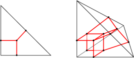
Figure 2: Tropical hyperplanes of dimensions $1$ and $2$ in tropical projective spaces.

Let $v\colon A\to{\mathbb{Z}}$ be the function defined by $v(m):=\operatorname{val}(k_{m})$. Let further $\Gamma_{v}$ be the subset in $M_{\mathbb{R}}\times{\mathbb{R}}$ defined by

$$\Gamma_{v}:=\{(m,r)\in A\times{\mathbb{R}}\,|\,r\leq v(m)\},$$

and $\operatorname{conv}(\Gamma_{v})$ be the convex hull of $\Gamma_{v}$ in $M_{\mathbb{R}}\times{\mathbb{R}}$. We write the polyhedral subdivision of $\Delta$ given by the projections of all bounded faces of $\operatorname{conv}(\Gamma_{v})$ to $M_{{\mathbb{R}}}$ as ${\mathcal{D}}_{v}$. Note that all vertices of any polyhedron in ${\mathcal{D}}_{v}$ are contained in $M$. It is well known that the tropical hypersurface $V_{\{0\}}(\operatorname{trop}(F))$ is dual to the polyhedral subdivision ${\mathcal{D}}_{v}$ [7, Proposition 3.1.6].

Definition 2.7.

The polyhedral subdivision ${\mathcal{D}}_{v}$ is unimodular if all elements of ${\mathcal{D}}_{v}$ are simplices of volume $\frac{1}{(n+1)!}$. We say $V(\operatorname{trop}(F))$ is smooth in this case.

Example 2.8.

Consider the polynomial $F=t^{-1}+x_{1}+x_{2}+x_{1}^{-1}x_{2}^{-1}$. In this case, the function $v$ is given by $v((0,0))=1$ and $v((1,0))=v((0,1))=v((-1,-1))=0$. The set $\operatorname{conv}(\Gamma_{v})$ and the polyhedral subdivision ${\mathcal{D}}_{v}$ are shown in Fig. 3. The polyhedral subdivision ${\mathcal{D}}_{v}$ is unimodular and $V(\operatorname{trop}(F))$ is smooth in this case.

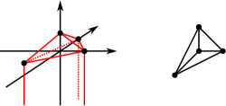
Figure 3: The set $\operatorname{conv}(\Gamma_{v})$ and the polyhedral subdivision ${\mathcal{D}}_{v}$ for $F=t^{-1}+x_{1}+x_{2}+x_{1}^{-1}x_{2}^{-1}$.

We set $v_{m}:=\operatorname{val}(k_{m})$ for $m\in A$. For each $\mu\in P_{\{0\}}$, we define the subset $A_{\mu}\subset A$ as the set of elements of $A$ to which the dominant terms of $F$ at $\mu$ corresponds:

$$A_{\mu}:=\big{\{}m\in A\,|\,v_{m}+m\cdot X=\operatorname{trop}(F)(X)\mathrm{\ for\ all\ }X\in\mu\cap O_{\{0\}}({\mathbb{T}})\big{\}}.$$ (2.2)

Lemma 2.9 ([8, Lemma 6.5]).

Assume that the dimension of $\mu\in P_{\{0\}}$ is $k$ $(0\leq k\leq n)$. If the tropical hypersurface $V(\operatorname{trop}(F))$ is smooth, then the number of elements of $A_{\mu}$ is $n+2-k$.

Assume that $V(\operatorname{trop}(F))$ is smooth. We fix a sufficiently large $R\in{\mathbb{R}}^{>0}$ such that $1/R$ is smaller than the radius of convergence of $k_{m}$ for all $m\in A$, and set $S_{R}^{1}:=\{z\in{\mathbb{C}}\,|\,|z|=R\}$. For $q\in S_{R}^{1}$, let $f_{q}\in{\mathbb{C}}\big{[}x^{\pm}_{1},\dots,x^{\pm}_{n+1}\big{]}$ be the Laurent polynomial obtained by substituting $1/q$ to $t$ in $F$. We write the closure of $\big{\{}x\in O_{\{0\}}({\mathbb{C}})\,|\,f_{q}(x)=0\big{\}}$ in $X_{{\mathcal{F}}^{\prime}}({\mathbb{C}})$ as $V_{q}$.

Let $\sigma\in{\mathcal{F}}^{\prime}$ be an $l$-dimensional cone. For $\mu\in P_{\sigma}$, let $\mu^{\prime}\in P_{\{0\}}$ be the cell such that $\mu=\mu^{\prime}\cap X_{{\mathcal{F}}^{\prime},\sigma}$. We assume that the dimension of $\mu^{\prime}$ is $k$. Here, we have $l\leq k$. We define standard coordinates on $O_{\sigma}({\mathbb{C}})$ and $O_{\sigma}({\mathbb{T}})$ with respect to $\mu$ as follows. First, we number all elements of $A_{\mu^{\prime}}$ from $0$ to $n+1-k$ and write them as $(m_{0},\dots,m_{n+1-k})$. We set

$$\tilde{x}_{i}:=q^{v_{m_{i}}}x^{m_{i}}/q^{v_{m_{0}}}x^{m_{0}},\qquad\widetilde{X}_{i}:=(v_{m_{i}}+{m_{i}}\cdot X)-(v_{m_{0}}+{m_{0}}\cdot X),$$

for $i=1,\dots,n+1-k$. Since $V(\operatorname{trop}(F))$ is smooth, we can extend $(\tilde{x}_{1},\dots,\tilde{x}_{n+1-k})$ and $(\widetilde{X}_{1},\dots,\widetilde{X}_{n+1-k})$ to $(\tilde{x}_{1},\dots,\tilde{x}_{n+1-l})$ and $(\widetilde{X}_{1},\dots,\widetilde{X}_{n+1-l})$ which form coordinate systems on $O_{\sigma}({\mathbb{C}})$ and $O_{\sigma}({\mathbb{T}})$ respectively by setting

$$\tilde{x}_{i}:=q^{a_{i}}\prod_{j=1}^{n+1}x_{j}^{b_{ij}},\qquad\widetilde{X}_{i}:=a_{i}+\sum_{j=1}^{n+1}b_{ij}X_{j},$$

for $i=n+2-k,\dots,n+1-l$. Here, numbers $a_{i}$ and $b_{ij}$ are appropriate integral numbers. We call $(\tilde{x}_{1},\dots,\tilde{x}_{n+1-l})$ and $(\widetilde{X}_{1},\dots,\widetilde{X}_{n+1-l})$ standard coordinates with respect to $\mu$. There are some ambiguities of them resulting from different numbering of $(m_{0},\dots,m_{n+1-k})$ and different choices of numbers $a_{i}$ and $b_{ij}$.

Let $H_{\mu}\colon({\mathbb{C}}^{\ast})^{n+1-l}\to({\mathbb{C}}^{\ast})^{n+1-l}$ be the map defined by

$$(x_{1},\dots,x_{n+1-l})\mapsto(\tilde{x}_{1},\dots,\tilde{x}_{n+1-l}),$$

and $M_{\mu}\colon{\mathbb{R}}^{n+1-l}\to{\mathbb{R}}^{n+1-l}$ be the map defined by

$$(X_{1},\dots,X_{n+1-l})\mapsto\big{(}\widetilde{X}_{1},\dots,\widetilde{X}_{n+1-l}\big{)}.$$

Then the following diagram is commutative.

$$\begin{CD}({\mathbb{C}}^{\ast})^{n+1-l}@>{H_{\mu}}>{}>({\mathbb{C}}^{\ast})^{n+1-l}\\ @V{\operatorname{Log}_{R}}V{}V@V{}V{\operatorname{Log}_{R}}V\\ {\mathbb{R}}^{n+1-l}@>{M_{\mu}}>{}>{\mathbb{R}}^{n+1-l},\end{CD}$$

where the map $\operatorname{Log}_{R}\colon({\mathbb{C}}^{\ast})^{n+1-l}\to{\mathbb{R}}^{n+1-l}$ is defined by

$$(x_{1},\dots,x_{n+1-l})\to(\log_{R}|x_{1}|,\dots,\log_{R}|x_{n+1-l}|).$$

Example 2.10.

Let us consider the polynomial $F=t^{-1}+x_{1}+x_{2}+x_{1}^{-1}x_{2}^{-1}$ again. We have $f_{q}=q+x_{1}+x_{2}+x_{1}^{-1}x_{2}^{-1}$. The tropicalization of $F$ is $\operatorname{trop}(F)=\max\{1,X_{1},X_{2},-X_{1}-X_{2}\}$. The tropical hypersurface defined by $\operatorname{trop}(F)$ is shown in Fig. 4. Let $\nu$ and $\mu$ denote the vertex and the edge of $V(\operatorname{trop}(F))$ as shown in Fig. 4. The set $A_{\nu}$ is given by $\{(0,0),(1,0),(-1,-1)\}$. We set $y_{1}:=x_{1}/q=q^{-1}x_{1}$, $y_{2}:=x_{1}^{-1}x_{2}^{-1}/q=q^{-1}x_{1}^{-1}x_{2}^{-1}$ and $Y_{1}:=-1+X_{1}$, $Y_{2}:=-1-X_{1}-X_{2}$. Then the sets of function $(y_{1},y_{2})$ and $(Y_{1},Y_{2})$ form standard coordinates with respect to $\nu$ on $O_{\{0\}}({\mathbb{C}})$ and $O_{\{0\}}({\mathbb{T}})$, respectively. The set $A_{\mu}$ is given by $\{(1,0),(-1,-1)\}$. We set $z_{1}:=x_{1}^{-1}x_{2}^{-1}/x_{1}=x_{1}^{-2}x_{2}^{-1}$ and $Z_{1}:=-2X_{1}-X_{2}$. For instance, if we set $z_{2}:=q^{2}x_{1}$ and $Z_{2}:=2+X_{1}$, then we have

$$\det\begin{pmatrix}-2&1\\ -1&0\end{pmatrix}=1.$$

Hence, the sets of functions $(z_{1},z_{2})$ and $(Z_{1},Z_{2})$ form standard coordinates with respect to $\mu$ on $O_{\{0\}}({\mathbb{C}})$ and $O_{\{0\}}({\mathbb{T}})$, respectively.

Figure 4: The tropical hypersurface defined by $\operatorname{trop}(F)=\max\{1,X_{1},X_{2},-X_{1}-X_{2}\}$.

3 Tropical localization

Tropical localization is a way to simplify algebraic hypersurfaces around the tropical limit points by ignoring terms which are not dominant in the tropical limit. This technique is first introduced by Mikhalkin [8]. In this section, we give a concrete defining function realizing the tropical localization based on the idea of Mikhalkin. There is also a similar construction of the tropical localization in [1].

Let $K:={\mathbb{C}}\{t\}$ be the convergent Laurent series field, equipped with the standard non-archimedean valuation (1.1). Let further $\Delta\subset M_{\mathbb{R}}$ be a convex lattice polytope. We set $A:=\Delta\cap M$. Let $F=\sum\limits_{m\in A}k_{m}x^{m}\in K\big{[}x^{\pm}_{1},\dots,x^{\pm}_{n+1}\big{]}$ be a polynomial over $K$ such that $k_{m}\neq 0$ for all $m\in A$. We set $v_{m}:=\operatorname{val}(k_{m})$. We fix a sufficiently large $R\in{\mathbb{R}}^{>0}$ such that $1/R$ is smaller than the radius of convergence of $k_{m}$ for all $m\in A$, and set $S_{R}^{1}:=\{z\in{\mathbb{C}}\,|\,|z|=R\}$. For $q\in S_{R}^{1}$, let $f_{q}\in{\mathbb{C}}\big{[}x^{\pm}_{1},\dots,x^{\pm}_{n+1}\big{]}$ denote the polynomial obtained by substituting $1/q$ to $t$ in $F$. Let ${\mathcal{F}}$ denote the normal fan to $\Delta$. We choose a unimodular subdivision ${\mathcal{F}}^{\prime}$ of ${\mathcal{F}}$. Let $V_{q}$ be the hypersurface in $X_{{\mathcal{F}}^{\prime}}({\mathbb{C}})$ defined by $f_{q}$. Let further $V(\operatorname{trop}(F))$ be the tropical hypersurface in $X_{{\mathcal{F}}^{\prime}}({\mathbb{C}})$ defined by $\operatorname{trop}(F)$ and $P$ be the polyhedral complex in $X_{{\mathcal{F}}^{\prime}}({\mathbb{T}})$ given by $V(\operatorname{trop}(F))$. Assume that $V(\operatorname{trop}(F))$ is smooth (see Definition 2.7).

Let $C_{0},C_{1}\in{\mathbb{R}}$ be constants such that $0<C_{1}<C_{0}\ll 1$. Let $b\colon{\mathbb{R}}\to{\mathbb{R}}$ be a monotone $C^{\infty}$ function on ${\mathbb{R}}$ satisfying following conditions:

1. $b(X)=1$ if and only if $X\leq C_{1}$,

2. $b(X)=0$ if and only if $X\geq C_{0}$.

The graph of the function $b$ is shown in Fig. 5.

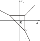
Figure 5: The graph of the function $b$.

We define the tropical localization of the hypersurface $V_{q}$ as follows.

Definition 3.1.

For each $m\in A$, let $b_{m}\colon O_{\{0\}}({\mathbb{C}})\to{\mathbb{R}}$ be the function defined by

$$b_{m}(x):=\prod_{i\in A}b\big{(}\log_{R}\big{|}q^{v_{i}}x^{i}\big{|}-\log_{R}\big{|}{q^{v_{m}}x^{m}}\big{|}\big{)}.$$

In addition, let $\tilde{f}_{q}\colon O_{\{0\}}({\mathbb{C}})\to{\mathbb{C}}$ be the function defined by

$$\tilde{f}_{q}(x):=\sum_{m\in A}b_{m}(x)q^{v_{m}}x^{m}.$$

We define the tropical localization $W_{q}$ of $V_{q}$ as the closure of $\{x\in O_{\{0\}}({\mathbb{C}})\,|\,\tilde{f}_{q}(x)=0\}$ in $X_{{\mathcal{F}}^{\prime}}({\mathbb{C}})$.

By applying Definition 3.1 to $f(x_{1},\dots,x_{n+1})=1+x_{1}+\dots+x_{n+1}$, we can construct the tropically localized hyperplane.

Definition 3.2.

We define the function $\tilde{f}\colon O_{\{0\}}({\mathbb{C}})\to{\mathbb{C}}$ by

$$\tilde{f}(x_{1},\dots,x_{n+1}):=\prod_{i=1}^{n+1}b(\log_{R}|x_{i}|)+\sum_{i=1}^{n+1}\left\{b(-\log_{R}|x_{i}|)\prod_{j=1}^{n+1}b(\log_{R}|x_{j}|-\log_{R}|x_{i}|)\right\}x_{i},$$

We call the submanifold defined as the zero locus of $\tilde{f}$ the tropically localized hyperplane.

Definition 3.3.

For each $\mu\in P$, we define $D_{\mu}\subset X_{{\mathcal{F}}^{\prime}}({\mathbb{C}})$ and $\widehat{D}_{\mu}\subset X_{{\mathcal{F}}^{\prime}}({\mathbb{T}})$ as follows. For $\mu\in P_{\{0\}}$, we define $D_{\mu}\subset X_{{\mathcal{F}}^{\prime}}({\mathbb{C}})$ and $\widehat{D}_{\mu}\subset X_{{\mathcal{F}}^{\prime}}({\mathbb{T}})$ by

$$D_{\mu}:=\overline{\left\{x\in O_{\{0\}}({\mathbb{C}})\left|\,\begin{array}[]{@{}l@{}}b_{m}(x)>0\ {\rm for\ }m\in A_{\mu},\\ b_{m}(x)=0\ {\rm for\ }m\in A\setminus A_{\mu}\\ \end{array}\right.\right\}},$$

$$\widehat{D}_{\mu}:=\overline{\left\{X\in O_{\{0\}}({\mathbb{T}})\left|\,\begin{array}[]{@{}l@{}}|(v_{m^{\prime}}+m^{\prime}\cdot X)-(v_{m}+m\cdot X)|<C_{0}\ {\rm for\ }m,m^{\prime}\in A_{\mu},\\ {\rm for\ any\ }m\in A\setminus A_{\mu},{\rm\ there\ exists\ }m^{\prime}\in A_{\mu}\\ {\rm such\ that\ }(v_{m^{\prime}}+m^{\prime}\cdot X)-(v_{m}+m\cdot X)\geq C_{0}\\ \end{array}\right.\right\}},$$

where $A_{\mu}\subset A$ is the set defined in (2.2) and the overlines mean the closure in $X_{{\mathcal{F}}^{\prime}}({\mathbb{C}})$ and $X_{{\mathcal{F}}^{\prime}}({\mathbb{T}})$, respectively.

For $\mu\in P_{\sigma}$ $(\sigma\neq\{0\})$, let $\mu^{\prime}\in P_{\{0\}}$ be the cell such that $\mu=\mu^{\prime}\cap X_{{\mathcal{F}}^{\prime},\sigma}({\mathbb{T}})$. We define $D_{\mu}\subset X_{{\mathcal{F}}^{\prime},\sigma}({\mathbb{C}})$ and $\widehat{D}_{\mu}\subset X_{{\mathcal{F}}^{\prime},\sigma}({\mathbb{T}})$ by

$$D_{\mu}:=D_{\mu^{\prime}}\cap X_{{\mathcal{F}}^{\prime},\sigma}({\mathbb{C}}),\qquad\widehat{D}_{\mu}:=\widehat{D}_{\mu^{\prime}}\cap X_{{\mathcal{F}}^{\prime},\sigma}({\mathbb{T}}).$$ (3.1)

The monomial $v_{m}+m\cdot X\ (m\in A_{\mu})$ of $\operatorname{trop}(F)$ corresponds to the monomial $k_{m}x^{m}$ of $F$. Hence, we have $D_{\mu}=(\operatorname{Log}_{R})^{-1}(\widehat{D}_{\mu})$ for any $\mu\in P$, where $\operatorname{Log}_{R}$ is the map from $X_{{\mathcal{F}}^{\prime}}({\mathbb{C}})$ to $X_{{\mathcal{F}}^{\prime}}({\mathbb{T}})$ defined in (2.1).

Example 3.4.

Consider the polynomial $F=t^{-1}+x_{1}+x_{2}+x_{1}^{-1}x_{2}^{-1}$. The tropical hypersurface $V(\operatorname{trop}(F))$ and the regions $\{\widehat{D}_{\mu}\}_{\mu\in P}$ for $F$ are shown in Figs. 7 and 7. $\nu_{i}$ and $\mu_{i}$ $(i=1,\dots,6)$ denote vertices and edges of $V(\operatorname{trop}(F))$ respectively as shown in Fig. 7. Each $\widehat{D}_{\nu_{i}}$ is the region colored in dark gray and each $\widehat{D}_{\mu_{i}}$ is the region colored in light gray as shown in Fig. 7.

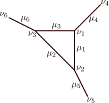
Figure 6: The tropical hypersurface $V(\operatorname{trop}(F))$ for $F=t^{-1}+x_{1}+x_{2}+x_{1}^{-1}x_{2}^{-1}$.

Figure 7: The regions $\{\widehat{D}_{\rho}\}_{\rho}$ for $F=t^{-1}+x_{1}+x_{2}+x_{1}^{-1}x_{2}^{-1}$.

Lemma 3.5.

If $C_{0}$ is sufficiently small, then $D_{\rho}\cap X_{{\mathcal{F}}^{\prime},\sigma}({\mathbb{C}})\neq\varnothing$ if and only if $\rho\cap X_{{\mathcal{F}}^{\prime},\sigma}({\mathbb{T}})\neq\varnothing$ for any $\rho\in P_{\{0\}}$ and $\sigma\in{\mathcal{F}}^{\prime}$.

Proof.

Assume that $\rho\cap X_{{\mathcal{F}}^{\prime},\sigma}({\mathbb{T}})\neq\varnothing$. We set $\mu:=\rho\cap X_{{\mathcal{F}}^{\prime},\sigma}({\mathbb{T}})$. We show that $\widehat{D}_{\mu}=\widehat{D}_{\rho}\cap X_{{\mathcal{F}}^{\prime},\sigma}({\mathbb{T}})\neq\varnothing$. If $C_{0}$ is sufficiently small, points in $\rho$ which are sufficiently far from all faces of $\rho$ in $P_{\{0\}}$ are contained in $\widehat{D}_{\rho}$. It follows that points in $\mu$ which are sufficiently far from all faces of $\mu$ are contained in $\widehat{D}_{\rho}$, and hence in $\widehat{D}_{\mu}$. Conversely, assume that $\rho\cap X_{{\mathcal{F}}^{\prime},\sigma}({\mathbb{T}})=\varnothing$. Since the region $\widehat{D}_{\rho}$ has to be near to the cell $\rho$ if $C_{0}$ is sufficiently small, we have $\widehat{D}_{\rho}\cap X_{{\mathcal{F}}^{\prime},\sigma}({\mathbb{T}})=\varnothing$. ∎

Lemma 3.6.

If $C_{0}$ is sufficiently small, then one has

$$\bigcup_{\rho\in P_{\{0\}}}D_{\rho}=\bigcup_{\sigma\in{\mathcal{F}}^{\prime}}\bigg{\{}\bigcup_{\mu\in P_{\sigma}}(D_{\mu}\cap O_{\sigma}({\mathbb{C}}))\bigg{\}}.$$

Proof.

It is obvious that the right-hand side is contained in the left-hand side. We show that the left-hand side is contained in the right-hand side. Let $x$ be any point in $D_{\rho}$ $(\rho\in P_{\{0\}})$. There exists the unique cone $\sigma\in{\mathcal{F}}^{\prime}$ such that $x\in O_{\sigma}({\mathbb{C}})$. Then, the point $x$ is contained in $D_{\rho}\cap X_{{\mathcal{F}}^{\prime},\sigma}({\mathbb{C}})$. From Lemma 3.5, we have $\rho\cap X_{{\mathcal{F}}^{\prime},\sigma}({\mathbb{T}})\neq\varnothing$. We set $\mu:=\rho\cap X_{{\mathcal{F}}^{\prime},\sigma}({\mathbb{T}})$. Then we have $D_{\rho}\cap X_{{\mathcal{F}}^{\prime},\sigma}({\mathbb{C}})=D_{\mu}$ from (3.1). Hence one has $x\in D_{\mu}\cap O_{\sigma}({\mathbb{C}})$. ∎

For each subset $\{m_{0},\dots,m_{p}\}\subset A\ (p\in{\mathbb{Z}}_{\geq 0})$, we define

$$D_{m_{0},\dots,m_{p}}:=\overline{\left\{x\in O_{\{0\}}({\mathbb{C}})\left|\,\begin{array}[]{@{}l@{}}b_{m_{i}}(x)>0\ {\rm for\ }i=0,\dots,p,\\ b_{m}(x)=0\ {\rm for\ }m\in A\setminus\{m_{0},\dots,m_{p}\}\\ \end{array}\right.\right\}},$$

where the overline means the closure in $X_{{\mathcal{F}}^{\prime}}({\mathbb{C}})$.

Lemma 3.7.

Let $\{m_{0},\dots,m_{p}\}$ be a subset of $A$ such that $p\geq 1$ and $\{m_{0},\dots,m_{p}\}\neq A_{\rho}$ for any $\rho\in P_{\{0\}}$. If the constant $C_{0}$ is sufficiently small, then one has $D_{m_{0},\dots,m_{p}}=\varnothing$.

Proof.

Let $H\subset O_{\{0\}}({\mathbb{T}})$ be the affine space defined by $v_{m_{0}}+m_{0}\cdot X=\dots=v_{m_{p}}+m_{p}\cdot X$. First, we show that there exists a neighborhood $N$ of $H$ such that any of $v_{m_{0}}+m_{0}\cdot X,\dots,v_{m_{p}}+m_{p}\cdot X$ do not coincide with $\operatorname{trop}(F)$ on $N$. Assume that there exists $X_{0}\in H$ and $i\in\{1,\dots,p\}$ such that $v_{m_{i}}+m_{i}\cdot X_{0}=\operatorname{trop}(F)(X_{0})$. Then there exists $\rho^{\prime}\in P_{\{0\}}$ such that $X_{0}\in\rho^{\prime}$ and $\{m_{0},\dots,m_{p}\}\subset A_{\rho^{\prime}}$. Since $V(\operatorname{trop}(F))$ is smooth and locally coincides with the tropical hyperplane, there exists $\rho\in P_{\{0\}}$ such that $\rho^{\prime}\prec\rho$ and $\{m_{0},\dots,m_{p}\}=A_{\rho}$. This contradicts to the assumption. Hence, any of $v_{m_{0}}+m_{0}\cdot X,\dots,v_{m_{p}}+m_{p}\cdot X$ do not coincide with $\operatorname{trop}(F)$ on $H$. Then there exists a neighborhood $N$ of $H$ such that any of $v_{m_{0}}+m_{0}\cdot X,\dots,v_{m_{p}}+m_{p}\cdot X$ do not coincide with $\operatorname{trop}(F)$ on $N$.

Assume that $D_{m_{0},\dots,m_{p}}$ is not empty. The differences between the values of $v_{m_{0}}+m_{0}\cdot X,\dots,v_{m_{p}}+m_{p}\cdot X$ are in the range of $\pm C_{0}$ on $\operatorname{Log}_{R}(D_{m_{0},\dots,m_{p}})\cap O_{\{0\}}({\mathbb{T}})$. Then the set $\operatorname{Log}_{R}(D_{m_{0},\dots,m_{p}})\cap O_{\{0\}}({\mathbb{T}})$ has to be in $N$ for a sufficiently small constant $C_{0}$. The fact that any of $v_{m_{0}}+m_{0}\cdot X,\dots,v_{m_{p}}+m_{p}\cdot X$ do not coincide with $\operatorname{trop}(F)$ on $N\supset\operatorname{Log}_{R}(D_{m_{0},\dots,m_{p}})\cap O_{\{0\}}({\mathbb{T}})$ contradicts to the definition of $D_{m_{0},\dots,m_{p}}$. ∎

Lemma 3.8.

Let $\sigma\in{\mathcal{F}}^{\prime}$ be a cone and $\mu_{1},\mu_{2}\in P_{\sigma}$ be cells. Suppose that the constant $C_{0}$ is sufficiently small. If $D_{\mu_{1}}\cap D_{\mu_{2}}\neq\varnothing$, then there exists $\mu\in P_{\sigma}$ such that $\mu\prec\mu_{1},\mu_{2}$ and $D_{\mu_{1}}\cap D_{\mu_{2}}\subset D_{\mu}$.

Proof.

Let $\mu_{1}^{\prime},\mu_{2}^{\prime}\in P_{\{0\}}$ be the cells such that $\mu_{1}=\mu_{1}^{\prime}\cap X_{{\mathcal{F}}^{\prime},\sigma}({\mathbb{T}})$ and $\mu_{2}=\mu_{2}^{\prime}\cap X_{{\mathcal{F}}^{\prime},\sigma}({\mathbb{T}})$. We set $\{m_{0},\dots,m_{p}\}:=A_{\mu_{1}^{\prime}}\cup A_{\mu_{2}^{\prime}}$. Here, we have $D_{\mu_{1}^{\prime}}\cap D_{\mu_{2}^{\prime}}\subset D_{m_{0},\dots,m_{p}}$. If $D_{\mu_{1}}\cap D_{\mu_{2}}\neq\varnothing$, the set $D_{\mu_{1}^{\prime}}\cap D_{\mu_{2}^{\prime}}\supset D_{\mu_{1}}\cap D_{\mu_{2}}$ is also nonempty. Hence, we have $D_{m_{0},\dots,m_{p}}\neq\varnothing$. From Lemma 3.7, there must exists a cell $\rho\in P_{\{0\}}$ such that $A_{\rho}=\{m_{0},\dots,m_{p}\}$ and $D_{m_{0},\dots,m_{p}}=D_{\rho}$. We have $D_{\mu_{1}^{\prime}}\cap D_{\mu_{2}^{\prime}}\subset D_{\rho}$ and $\rho\prec\mu_{1}^{\prime},\mu_{2}^{\prime}$. Then the cell $\mu:=\rho\cap X_{{\mathcal{F}}^{\prime},\sigma}({\mathbb{T}})$ satisfies $D_{\mu_{1}}\cap D_{\mu_{2}}\subset D_{\mu}$ and $\mu\prec\mu_{1},\mu_{2}$. ∎

The aim of this section is to prove the following theorem.

Theorem 3.9.

Fix a sufficiently small constant $C_{0}$. For a sufficiently large $R\in{\mathbb{R}}^{>0}$, the tropical localization $W_{q}$ and the family of subsets $\{D_{\mu}\}_{\mu\in P}$ of $X_{{\mathcal{F}}^{\prime}}({\mathbb{C}})$ satisfy the following conditions:

1. For any $q\in S_{R}^{1}$, the submanifold $W_{q}$ is isotopic to $V_{q}$ in $X_{{\mathcal{F}}^{\prime}}({\mathbb{C}})$.

2. For any $q\in S_{R}^{1}$, one has $W_{q}\subset\bigcup_{\rho\in P_{\{0\}}}D_{\rho}$.

3. Let $\sigma\in{\mathcal{F}}^{\prime}$ be a cone and $\mu\in P_{\sigma}$ be a cell. Let further $\mu^{\prime}\in P_{\{0\}}$ be the cell such that $\mu=\mu^{\prime}\cap X_{{\mathcal{F}}^{\prime},\sigma}({\mathbb{T}})$. Assume that the dimension of $\sigma$ and $\mu^{\prime}$ is $l$ and $k$, respectively $(l\leq k)$. Let $(\tilde{x}_{1},\dots,\tilde{x}_{n+1-l})$ be a standard coordinate with respect to $\mu$ $($see Section 2.3). Then, the defining equation of $W_{q}$ on $D_{\mu}\cap O_{\sigma}({\mathbb{C}})$ coincides with that of the $(n-k)$-dimensional tropically localized hyperplane in $(\tilde{x}_{1},\dots,\tilde{x}_{n+1-k})$ and is independent of the coordinate $(\tilde{x}_{n+2-k},\dots,\tilde{x}_{n+1-l})$.

The outline of the proof of Theorem 3.9 is as follows. In order to show the condition 1, we construct an isotopy $\{V_{q,s}\}_{s\in[0,1]}$ which connects $V_{q}$ and $W_{q}$. For $F=\sum\limits_{m\in A}k_{m}x^{m}$, we set $k_{m}=\sum\limits_{i\in{\mathbb{Z}}}c_{mi}t^{i}\in K$ $(c_{mi}\in{\mathbb{C}})$ and $c_{m}:=c_{m,-v_{m}}$. Let $d(s)$ be a real valued monotone $C^{\infty}$ function on ${\mathbb{R}}$ which has $1$ on $\{s\geq 2/3\}$ and $0$ on $\{s\leq 1/3\}$. The graph of $d(s)$ is shown in Fig. 8. For each $s\in[0,1]$, we define the functions $b_{m,s}\colon O_{\{0\}}({\mathbb{C}})\to{\mathbb{R}}$ and $\tilde{f}_{q,s}\colon O_{\{0\}}({\mathbb{C}})\to{\mathbb{C}}$ by

$$b_{m,s}(x):=(1-d(s))+d(s)b_{m}(x),$$

$$\tilde{f}_{q,s}(x):=\sum_{m\in A}b_{m,s}(x){c_{m}}^{(1-d(s))}q^{v_{m}}x^{m}+(1-d(s))\left\{f_{q}-\sum_{m\in A}{c_{m}}q^{v_{m}}x^{m}\right\},$$

where the branch of $c_{m}^{(1-d(s))}$ is determined by $0\leq\arg(c_{m})<2\pi$. Let $V_{q,s}$ be the closure of $\{x\in O_{\{0\}}({\mathbb{C}})\,|\,\tilde{f}_{q,s}(x)=0\}$ in $X_{{\mathcal{F}}^{\prime}}({\mathbb{C}})$. Then we have $\tilde{f}_{q,0}=f_{q},\tilde{f}_{q,1}=\tilde{f}_{q}$ and $V_{q,0}=V_{q}$, $V_{q,1}=W_{q}$.

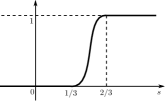
Figure 8: The graph of the function $d$.

First, we check that $V_{q,s}$ is contained in $\bigcup_{\rho\in P_{\{0\}}}D_{\rho}$ for any $q\in S_{R}^{1}$ and $s\in[0,1]$. Then, we set $q=R\exp(\sqrt{-1}\theta)$ and consider the projection $p\colon X_{{\mathcal{F}}^{\prime}}({\mathbb{C}})\times(-\epsilon,2\pi+\epsilon)\times(0,1)\to(-\epsilon,2\pi+\epsilon)\times(0,1)$ given by

$$(x,\theta,s)\mapsto(\theta,s),$$

where $\epsilon\in{\mathbb{R}}$ is a small constant such that $0<\epsilon\ll 1$. Let $Y$ be the subset of $X_{{\mathcal{F}}^{\prime}}({\mathbb{C}})\times(-\epsilon,2\pi+\epsilon)\times(0,1)$ defined by

$$Y:=\big{\{}(x,\theta,s)\in X_{{\mathcal{F}}^{\prime}}({\mathbb{C}})\times(-\epsilon,2\pi+\epsilon)\times(0,1)\,|\,\tilde{f}_{q,s}(x)=0\big{\}}.$$

We use the following theorem.

Theorem 3.10 (Ehresmann’s fibration theorem).

Let $f\colon E\to M$ be a $C^{\infty}$ map between smooth manifolds. If the map $f$ is a proper submersion, then the map $f$ is a locally trivial fibration.

We check that the function $\tilde{f}_{q,s}$ has $0$ as a regular value on each $D_{\mu}\cap O_{\sigma}({\mathbb{C}})$ for any $q\in S_{R}^{1}$ and $s\in[0,1]$. Then, it turns out that the restriction of $p$ to $Y$ is a submersion. In addition, we can easily see that $p|_{Y}$ is proper. From Theorem 3.10, we can conclude that the family of submanifolds $\{V_{q,s}\}_{s\in[0,1]}$ gives an isotopy between $V_{q}$ and $W_{q}$. The condition 3 can be shown by a simple calculation.

Proof of Theorem 3.9.

We set $T:=\bigcup_{\rho\in P_{\{0\}}}D_{\rho}$. First, we show that $V_{q,s}$ is contained in $T$ for any $q\in S_{R}^{1}$ and $s\in[0,1]$. Since we have

$$O_{\{0\}}({\mathbb{C}})=\Bigg{(}\bigcup_{\begin{subarray}{c}\{m_{0},\dots m_{p}\}\subset A\\ p\in{\mathbb{Z}}^{\geq 0}\end{subarray}}D_{m_{0},\dots,m_{p}}\Bigg{)}\cap O_{\{0\}}({\mathbb{C}}),$$

it follows from Lemma 3.7 that it is enough to check that the function $\tilde{f}_{q,s}$ can not be $0$ on $D_{m}\cap O_{\{0\}}({\mathbb{C}})$ for any $m\in A$. The dominant term of $\tilde{f}_{q,s}$ on $D_{m}\cap O_{\{0\}}({\mathbb{C}})$ is only ${c_{m}}^{(1-d(s))}q^{v_{m}}x^{m}$ and we have

$$b_{m^{\prime},s}(x)=\begin{cases}1-d(s),&m^{\prime}\neq m,\\ 1&m^{\prime}=m.\end{cases}$$

Hence, the function $\tilde{f}_{q,s}$ can be written on $D_{m}\cap O_{\{0\}}({\mathbb{C}})$ as

$${c_{m}}^{(1-d(s))}q^{v_{m}}x^{m}+(1-d(s))\bigg{\{}\sum_{p}h_{p}q^{i_{p}}x^{j_{p}}\bigg{\}},$$

where $h_{p}\in{\mathbb{C}}$, $i_{p}\in{\mathbb{Z}}$, $j_{p}\in A$ and each term $h_{p}q^{i_{p}}x^{j_{p}}$ denotes other monomial which is not dominant on $D_{m}$, i.e., $|q^{i_{p}}x^{j_{p}}|/|q^{v_{m}}x^{m}|\leq R^{-C_{0}}$. (Each index $p$ satisfies that either $j_{p}\neq m$ or $j_{p}=m$ and $i_{p}<v_{m}$.) Hence, for sufficiently large $R$, the function $\tilde{f}_{q,s}$ can not be $0$ on $D_{m}\cap O_{\{0\}}({\mathbb{C}})$. Then we have $V_{q,s}\subset T$ for all $q\in S_{R}^{1}$ and $s\in[0,1]$. In particular, the condition 2 holds.

Next, we show that the projection $\left.p\right|_{Y}$ is a proper submersion. For $\mu\in P_{\sigma}$, let $\mu^{\prime}\in P_{\{0\}}$ be the cell such that $\mu=\mu^{\prime}\cap X_{{\mathcal{F}}^{\prime},\sigma}$. We define $m_{0},\dots,m_{n+1-k}$ by $\{m_{0},\dots,m_{n+1-k}\}=A_{\mu^{\prime}}$ (the set $A_{\mu^{\prime}}$ is defined in (2.2)). For any $m\in A\setminus A_{\mu^{\prime}}$, there exists $m_{i}\in A_{\mu^{\prime}}$ such that $|q^{v_{m}}x^{m}|/|{q^{v_{m_{i}}}x^{m_{i}}}|\leq R^{-C_{0}}$ on $D_{\mu^{\prime}}\cap O_{\{0\}}({\mathbb{C}})$. Then we have $b\big{(}\log_{R}|q^{v_{m}}x^{m}|-\log_{R}|{q^{v_{m_{i}}}x^{m_{i}}}|\big{)}\equiv 1$ and $b\big{(}\log_{R}|q^{v_{m_{i}}}x^{m_{i}}|-\log_{R}|{q^{v_{m}}x^{m}}|\big{)}\equiv 0$. Therefore, we have

$$b_{m,s}|_{D_{\mu^{\prime}}\cap O_{\{0\}}({\mathbb{C}})}(x)$$

$$\qquad{}=\begin{cases}(1-d(s))+d(s)\prod\limits_{i=0}^{n+1-k}b\big{(}\log_{R}|q^{v_{m_{i}}}x^{m_{i}}|-\log_{R}|{q^{v_{m}}x^{m}}|\big{)},&m\in A_{\mu^{\prime}},\\ 1-d(s)&\mathrm{otherwise,}\end{cases}$$

and

$$\tilde{f}_{q,s}\big{|}_{D_{\mu^{\prime}}\cap O_{\{0\}}({\mathbb{C}})}(x)=\sum_{i=0}^{n+1-k}b_{m_{i},s}(x)c_{m_{i}}^{(1-d(s))}q^{v_{m_{i}}}x^{m_{i}}$$

$$\hphantom{\tilde{f}_{q,s}\big{|}_{D_{\mu^{\prime}}\cap O_{\{0\}}({\mathbb{C}})}(x)=}{}+(1-d(s))\bigg{\{}f_{q}-\sum_{m\in A}{c_{m}}q^{v_{m}}x^{m}+\sum_{m\in A\setminus A_{\mu^{\prime}}}{c_{m}}^{(1-d(s))}q^{v_{m}}x^{m}\bigg{\}}.$$ (3.2)

Let $\tau\in{\mathcal{F}}^{\prime}$ be an $(n+1)$-dimensional cone having $\sigma$ as its face. Let further $e_{1},\dots,e_{n+1}\in{\mathbb{Z}}^{n+1}$ be the primitive generators of $\tau^{\vee}$. We rearrange $e_{1},\dots,e_{n+1}$ if necessary, and set $y_{i}:=x^{e_{i}}$ $(i=1,\dots,n+1)$ so that the set of functions $(y_{1},\dots,y_{n+1})$ forms a coordinate system on $U_{\tau}({\mathbb{C}})\cong{\mathbb{C}}^{n+1}$ such that $y_{n+2-l}=\cdots=y_{n+1}=0$ on $O_{\sigma}({\mathbb{C}})$. Let $(\tilde{x}_{1},\dots,\tilde{x}_{n+1-l})$ be a standard coordinate with respect to $\mu$ such that $\tilde{x}_{i}:=q^{v_{m_{i}}}x^{m_{i}}/q^{v_{m_{0}}}x^{m_{0}}$ for $i=1,\dots,n+1-k$. Then, the set of functions $(\tilde{x}_{1},\dots,\tilde{x}_{n+1-l},y_{n+2-l},\dots,y_{n+1})$ forms a coordinate system on $\bigcup_{\sigma^{\prime}\prec\sigma}O_{\sigma^{\prime}}({\mathbb{C}})$. We define the functions $b_{m_{i},\mu}\colon O_{\{0\}}({\mathbb{C}})\to{\mathbb{R}}$ by

$$b_{m_{0},\mu}(\tilde{x}):=\prod_{j=1}^{n+1-k}b(\log_{R}|\tilde{x}_{j}|),$$

$$b_{m_{i},\mu}(\tilde{x}):=b(-\log_{R}|\tilde{x}_{i}|)\prod_{j=1}^{n+1-k}b(\log_{R}|\tilde{x}_{j}|-\log_{R}|\tilde{x}_{i}|)\qquad\mathrm{for}\ \ i=1,\dots,n+1-k,$$

and set $b_{m_{i},\mu,s}(\tilde{x}):=(1-d(s))+d(s)b_{m_{i},\mu}(\tilde{x})$. In the coordinate system $(\tilde{x}_{1},\dots,\tilde{x}_{n+1-l},y_{n+2-l}$, $\dots,y_{n+1})$, we divide (3.2) by $q^{m_{0}}x^{m_{0}}$ to obtain

$$\frac{\tilde{f}_{q,s}\big{|}_{D_{\mu^{\prime}}\cap O_{\{0\}}({\mathbb{C}})}}{q^{m_{0}}x^{m_{0}}}=b_{m_{0},\mu,s}(\tilde{x})c_{m_{0}}^{(1-d(s))}\!+\!\sum_{i=1}^{n+1-k}\!\!b_{m_{i},\mu,s}(\tilde{x})c_{m_{i}}^{(1-d(s))}\tilde{x}_{i}+(1-d(s))\{\mathrm{other\ terms}\}.$$

Notice that other terms are not dominant on $D_{\mu^{\prime}}$. Hence, we may assume that the subset $V_{q,s}$ is defined on $D_{\mu}\cap O_{\sigma}({\mathbb{C}})$ by

$$b_{m_{0},\mu,s}(\tilde{x})c_{m_{0}}^{(1-d(s))}+\sum_{i=1}^{n+1-k}b_{m_{i},\mu,s}(\tilde{x})c_{m_{i}}^{(1-d(s))}\tilde{x}_{i}+(1-d(s))\bigg{\{}\sum_{p}h_{p}q^{i_{p}}\tilde{x}^{j_{p}}\bigg{\}}=0,$$ (3.3)

where $h_{p}\in{\mathbb{C}}$ and terms $\sum_{p}h_{p}q^{i_{p}}\tilde{x}^{j_{p}}$ denote other terms which are not dominant on $D_{\mu}$. We have $\big{|}q^{i_{p}}\tilde{x}^{j_{p}}\big{|}\leq R^{-C_{0}}$ and $\big{|}q^{i_{p}}\tilde{x}^{j_{p}}\big{|}/|\tilde{x}_{i}|\leq R^{-C_{0}}$ for all $p$. Let $G(\tilde{x}_{1},\dots,\tilde{x}_{n+1-l})$ denote the left-hand side of (3.3). We show that $G(\tilde{x}_{1},\dots,\tilde{x}_{n+1-l})$ has $0\in{\mathbb{C}}$ as a regular value on $D_{\mu}\cap O_{\sigma}({\mathbb{C}})$.

We define the subset $D_{\mu,m_{i}}:=\{x\in D_{\mu}\,|\,|q^{v_{m_{i}}}x^{m_{i}}|/|q^{v_{m_{j}}}x^{m_{j}}|\geq 1\ (j=0,\dots,n+1-k)\}$ for $i=0,\dots,n+1-k$. For any $x\in D_{\mu}$, there exists $i\in\{1,\dots n+1-k\}$ such that $|q^{v_{m_{i}}}x^{m_{i}}|\geq|q^{v_{m_{j}}}x^{m_{j}}|$ for any $j\in\{1,\dots,n+1-k\}$. Then we have $D_{\mu}=\bigcup_{i=0}^{n+1-k}D_{\mu,m_{i}}$. We have only to show that the Jacobian matrix of $G(\tilde{x}_{1},\dots,\tilde{x}_{n+1-l})$ has the maximal rank on $D_{\mu,{m_{1}}}$. On $D_{\mu,{m_{1}}}$, we have $b_{m_{1},\mu,s}(\tilde{x})\equiv 1$. We set $\tilde{x}_{i}=r_{i}\exp(\sqrt{-1}\theta_{i})\ (r_{i}\in{\mathbb{R}}^{\geq 0},\theta_{i}\in[0,2\pi])$ and let $M$ be a $2\times 2$ matrix defined by

$$M:=\begin{pmatrix}\dfrac{\partial}{\partial r_{1}}\operatorname{Re}(G)&\dfrac{\partial}{\partial\theta_{1}}\operatorname{Re}(G)\vspace{1mm}\\ \dfrac{\partial}{\partial r_{1}}\operatorname{Im}(G)&\dfrac{\partial}{\partial\theta_{1}}\operatorname{Im}(G)\end{pmatrix}.$$

We can show $\det(M)\neq 0$ for a sufficiently large $R$ by the concrete calculation. Hence, the subsets $V_{q,s}$ and $Y$ is smooth submanifold in $X_{{\mathcal{F}}^{\prime}}({\mathbb{C}})$ and $\{X_{{\mathcal{F}}^{\prime}}({\mathbb{C}})\times(-\epsilon,2\pi+\epsilon)\times(0,1)\}$ respectively. Moreover, it turns out that the projection $p|_{Y}\colon Y\to(-\epsilon,2\pi+\epsilon)\times(0,1)$ is a submersion.

In addition, for any compact subset $C\subset(-\epsilon,2\pi+\epsilon)\times(0,1)$, the inverse image $(p|_{Y})^{-1}(C)\subset Y$ coincides with $\{(x,\theta,s)\in X_{{\mathcal{F}}^{\prime}}({\mathbb{C}})\times C\,|\,\tilde{f}_{q,s}(x)=0\}$. Then the set $(p|_{Y})^{-1}(C)$ is compact and the map $p|_{Y}$ is proper. Hence, it turns out from Theorem 3.10 that the map $p|_{Y}$ has a structure of a fiber bundle with the fiber $V_{R,1}=W_{q=R}=:W_{R}$. Therefore, the family of submanifolds $\{V_{q,s}\}_{s\in[0,1]}$ gives an isotopy and the condition 1 holds.

Finally, we check the condition 3. In (3.3), we set $s=1$ to obtain

$$\prod_{j=1}^{n+1-k}b(\log_{R}|\tilde{x}_{j}|)+\sum_{i=1}^{n+1-k}\bigg{\{}b(-\log_{R}|\tilde{x}_{i}|)\prod_{j=1}^{n+1-k}b(\log_{R}|\tilde{x}_{j}|-\log_{R}|\tilde{x}_{i}|)\bigg{\}}\tilde{x}_{i}=0.$$

This coincides with the defining function of the $(n-k)$-dimensional tropically localized hyperplane in $(\tilde{x}_{1},\dots,\tilde{x}_{n+1-k})$ and the left-hand side is independent of the values of $\tilde{x}_{n+2-k},\dots$, $\tilde{x}_{n+1-l}$. Hence, the condition 3 holds. ∎

4 Monodromy transformations

We use the same notation as in Section 3 and keep the assumption that $V(\operatorname{trop}(F))$ is smooth. We set $W_{R}:=W_{q=R}$. Let $\{\psi_{q=R\exp(\sqrt{-1}\theta)}\colon W_{R}\to W_{q}\}_{\theta\in[0,2\pi]}$ be a family of homeomorphisms which depends on $\theta$ continuously. It is clear that the map $\psi_{q=R\exp(2\pi\sqrt{-1})}\colon W_{R}\to W_{R}$ gives the monodromy transformation of $\{V_{q}\}_{q\in S_{R}^{1}}$ under the identification $W_{R}\cong V_{R}$. Hence, it is sufficient to construct a monodromy transformation of $\{W_{q}\}_{q\in S_{R}^{1}}$ in order to get that of $\{V_{q}\}_{q\in S_{R}^{1}}$.

Proposition 4.1.

There exists a continuous map $\phi\colon\operatorname{Log}_{R}(W_{R})\to V(\operatorname{trop}(F))$ satisfying the following condition:

• $\phi(\operatorname{Log}_{R}(W_{R})\cap\widehat{D}_{\rho}\cap O_{\sigma}({\mathbb{T}}))\subset\rho\cap O_{\sigma}({\mathbb{T}})$ for any $\sigma\in{\mathcal{F}}^{\prime}$ and $\rho\in P_{\sigma}$.

Moreover, such maps are unique up to homotopy.

Proof.

For each cell $\rho\in P$, we construct a continuous map $\phi_{\rho}\colon\operatorname{Log}_{R}(W_{R})\cap\widehat{D}_{\rho}\to V(\operatorname{trop}(F))$ satisfying following conditions:

1. $\phi_{\rho}(\operatorname{Log}_{R}(W_{R})\cap\widehat{D}_{\rho}\cap O_{\sigma}({\mathbb{T}}))\subset\rho\cap O_{\sigma}({\mathbb{T}})$, where $\sigma\in{\mathcal{F}}^{\prime}$ is a cone such that $\rho\in P_{\sigma}$.

2. For any face $\mu\prec\rho$, the map $\phi_{\rho}$ coincides with $\phi_{\mu}$ on $\operatorname{Log}_{R}(W_{R})\cap\widehat{D}_{\rho}\cap\widehat{D}_{\mu}$.

We construct $\phi_{\rho}$ in an ascending order of $\dim\rho$ as follows. For each vertex $\rho\in P$, we set $\phi_{\rho}$ as a constant map from $\operatorname{Log}_{R}(W_{R})\cap\widehat{D}_{\rho}$ to $\rho$. For each $1$-cell $\rho$, let $\nu_{0}$ and $\nu_{1}$ be the endpoints of $\rho$. We set each $\phi_{\rho}$ as a continuous map to $\rho$ so that $\phi_{\rho}$ coincides with the constant map to $\nu_{i}$ on $\operatorname{Log}_{R}(W_{R})\cap\widehat{D}_{\rho}\cap\widehat{D}_{\nu_{i}}$ and satisfies the condition (i). Assume that we have constructed $\phi_{\rho}$ for all cells whose dimensions are lower than $k-1$. For each $k$-cell $\rho$, we define $\phi_{\rho}$ as a continuous map to $\rho$ so that $\phi_{\rho}$ coincides with $\phi_{\mu}$ on $\operatorname{Log}_{R}(W_{R})\cap\widehat{D}_{\rho}\cap\widehat{D}_{\mu}$ for any face $\mu$ of $\rho$ and satisfies the condition (i). In this way, we can construct a family of maps $\{\phi_{\rho}\}_{\rho\in P}$ such that each map $\phi_{\rho}$ satisfies the condition (i) and (ii).

Example 4.2.

Consider the polynomial $F=1+x_{1}+x_{2}$. Fig. 10 shows $V(\operatorname{trop}(F))$ and $\operatorname{Log}_{R}(W_{R})$. Let $\nu$ denote the center vertex of $V(\operatorname{trop}(F))$. The region colored gray denotes $\operatorname{Log}_{R}(W_{R})\cap\widehat{D}_{\nu}$. The map $\phi_{\nu}\colon\operatorname{Log}_{R}(W_{R})\cap\widehat{D}_{\nu}\to V(\operatorname{trop}(F))$ is the constant map to $\nu$ as shown in Fig. 10.

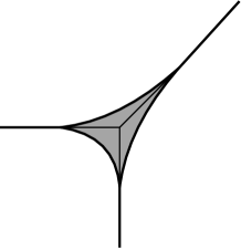
Figure 9: The region $\operatorname{Log}_{R}(W_{R})$ for $F=1+x_{1}+x_{2}$.

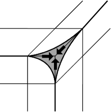
Figure 10: The map $\phi_{\nu}$ for $F=1+x_{1}+x_{2}$.

For any $\sigma\in{\mathcal{F}}^{\prime}$ and $\rho_{1},\rho_{2}\in P_{\sigma}$, if $\widehat{D}_{\rho_{1}}\cap\widehat{D}_{\rho_{2}}\neq\varnothing$, there exists $\rho\in P_{\sigma}$ such that $\rho\prec\rho_{1},\rho_{2}$ and $\widehat{D}_{\rho_{1}}\cap\widehat{D}_{\rho_{2}}\subset\widehat{D}_{\rho}$ (Lemma 3.8). From the condition (ii), the map $\phi_{\rho_{i}}$ coincides with $\phi_{\rho}$ on $\operatorname{Log}_{R}(W_{R})\cap\widehat{D}_{\rho}\cap\widehat{D}_{\rho_{i}}$ $(i=1,2)$. Hence, the maps $\phi_{\rho_{1}}$ and $\phi_{\rho_{2}}$ coincide with each other on $\operatorname{Log}_{R}(W_{R})\cap\widehat{D}_{\rho}\cap\widehat{D}_{\rho_{1}}\cap\widehat{D}_{\rho_{2}}$=$\operatorname{Log}_{R}(W_{R})\cap\widehat{D}_{\rho_{1}}\cap\widehat{D}_{\rho_{2}}$. Then it turns out that we can get the continuous map $\phi\colon\operatorname{Log}_{R}(W_{R})\to V(\operatorname{trop}(F))$ by gluing $\{\phi_{\rho}\}_{\rho}$. The map $\phi$ satisfies the condition $(\ast)$.

Let $\phi_{0},\phi_{1}\colon\operatorname{Log}_{R}(W_{R})\to V(\operatorname{trop}(F))$ be two maps satisfying the condition $(\ast)$. We construct a family of continuous maps $\{\phi_{s}\colon\operatorname{Log}_{R}(W_{R})\to X_{{\mathcal{F}}^{\prime}}({\mathbb{T}})\}_{s\in[0,1]}$ by $\phi_{s}(X):=(1-s)\phi_{0}(X)+s\phi_{1}(X)$, where the addition and the multiplications are taken on $O_{\sigma}({\mathbb{T}})\cong{\mathbb{R}}^{l}$ for the cone $\sigma\in{\mathcal{F}}^{\prime}$ such that $X\in O_{\sigma}({\mathbb{T}})$. This construction is independent of the choice of coordinates on $O_{\sigma}({\mathbb{T}})$. Since each cell is convex, $\phi_{s}$ satisfies the condition $(\ast)$ for any $s\in[0,1]$. Therefore, each map $\phi_{s}$ is well-defined as a continuous map to $V(\operatorname{trop}(F))$ and $\{\phi_{s}\}_{s\in[0,1]}$ gives a homotopy between $\phi_{0}$ and $\phi_{1}$. ∎

We fix a map $\phi\colon\operatorname{Log}_{R}(W_{R})\to V(\operatorname{trop}(F))$ satisfying the condition $(\ast)$ in Proposition 4.1. Let $\sigma\in{\mathcal{F}}^{\prime}$ be an $l$-dimensional cone. We choose $a_{i},b_{ij}\in{\mathbb{Z}}$ $(i=1,\dots,n+1-l$, $j=1,\dots,n+1)$ so that the sets of functions $(y_{1},\dots,y_{n+1-l})$ and $(Y_{1},\dots,Y_{n+1-l})$ defined by

$$y_{i}:=q^{a_{i}}\prod_{j=1}^{n+1}x_{j}^{b_{ij}},\qquad Y_{i}:=a_{i}+\sum_{j=1}^{n+1}b_{ij}X_{j},$$ (4.1)

form coordinate systems on $O_{\sigma}({\mathbb{C}})$ and $O_{\sigma}({\mathbb{T}})$, respectively. For each $q=R\exp(\sqrt{-1}\theta)\in S_{R}^{1}$, we define the map $\psi_{\sigma,q}\colon W_{R}\cap O_{\sigma}({\mathbb{C}})\to O_{\sigma}({\mathbb{C}})$ by

$$(y_{1},\dots,y_{n+1-l})\mapsto\big{(}\tilde{\phi}_{1,\theta}y_{1},\dots,\tilde{\phi}_{n+1-l,\theta}y_{n+1-l}\big{)},$$

where $\tilde{\phi}_{i,\theta}(y_{1},\dots,y_{n+1-l}):=\exp\left(\sqrt{-1}\theta Y_{i}\circ\phi\circ\operatorname{Log}_{R}(y)\right)$ $(i=1,\dots,n+1-l)$.

Lemma 4.3.

For any $q\in S_{R}^{1}$ and $\sigma\in{\mathcal{F}}^{\prime}$, the map $\psi_{\sigma,q}$ is independent of the choice of the coordinate system $(y_{1},\dots,y_{n+1-l})$ on $O_{\sigma}({\mathbb{C}})$ and the image $\psi_{\sigma,q}(W_{R}\cap O_{\sigma}({\mathbb{C}}))$ is contained in $W_{q}\cap O_{\sigma}({\mathbb{C}})$.

Proof.

First, we show that the map $\psi_{\sigma,q}$ is independent of the choice of the coordinate. Let $(z_{1},\dots,z_{n+1-l})$ and $(Z_{1},\dots,Z_{n+1-l})$ be other coordinate systems on $O_{\sigma}({\mathbb{C}})$ and $O_{\sigma}({\mathbb{T}})$ defined just as $(y_{1},\dots,y_{n+1-l})$ and $(Y_{1},\dots,Y_{n+1-l})$. We can write

$$z_{i}=q^{\alpha_{i}}\prod_{j=1}^{n+1-l}y_{j}^{\beta_{ij}},\qquad y_{i}=\prod_{j=1}^{n+1-l}\big{(}q^{-\alpha_{j}}z_{j}\big{)}^{\gamma_{ij}},$$

where $\alpha_{i},\beta_{ij}$ are some integral numbers. Here, we have $\sum\limits_{j=1}^{n+1-l}\beta_{ij}\gamma_{jk}=\delta_{ik}$. Let $\psi_{\sigma,q}^{\prime}\colon W_{R}\cap O_{\sigma}({\mathbb{C}})\to O_{\sigma}({\mathbb{C}})$ be the map defined in $(z_{1},\dots,z_{n+1-l})$. For all $z=(z_{1},\dots,z_{n+1-l})=y=(y_{1},\dots,y_{n+1-l})\in W_{R}\cap O_{\sigma}({\mathbb{C}})$, we have

$$z_{i}\left(\psi_{\sigma,q}^{\prime}(z)\right)=\left\{\exp\left(\sqrt{-1}\theta\left(\alpha_{i}+\sum_{j=1}^{n+1-l}\beta_{ij}Y_{j}\right)\left(\phi\circ\operatorname{Log}_{R}(z)\right)\right)\right\}R^{\alpha_{i}}\prod_{j=1}^{n+1-l}y_{j}^{\beta_{ij}},$$

and

$$y_{i}\left(\psi_{\sigma,q}^{\prime}(z)\right)=\prod_{k=1}^{n+1-l}\big{(}q^{-\alpha_{k}}z_{k}(\psi_{\sigma,q}^{\prime}(z))\big{)}^{\gamma_{ik}}$$

$$=\prod_{k=1}^{n+1-l}\left[q^{-\alpha_{k}}\left\{\exp\left(\sqrt{-1}\theta\left(\alpha_{k}+\sum_{j=1}^{n+1-l}\beta_{kj}Y_{j}\right)\left(\phi\circ\operatorname{Log}_{R}(z)\right)\right)\right\}R^{\alpha_{k}}\prod_{j=1}^{n+1-l}y_{j}^{\beta_{kj}}\right]^{\gamma_{ik}}$$

$$=\left\{\exp\left(\sqrt{-1}\theta\sum_{k,j}\gamma_{ik}\beta_{kj}Y_{j}\left(\phi\circ\operatorname{Log}_{R}(y)\right)\right)\right\}\prod_{j=1}^{n+1-l}y_{j}^{\sum_{k}\gamma_{ik}\beta_{kj}}$$

$$=\exp\left(\sqrt{-1}\theta Y_{i}\left(\phi\circ\operatorname{Log}_{R}(y)\right)\right)y_{i}=\tilde{\phi}_{i,\theta}y_{i}.$$

Therefore, we have $y_{i}(\psi_{\sigma,q}^{\prime}(y))=y_{i}(\psi_{\sigma,q}(y))=\tilde{\phi}_{i,\theta}y_{i}$. Hence, one has $\psi_{\sigma,q}=\psi_{\sigma,q}^{\prime}$.

Next, we show that the image $\psi_{\sigma,q}(W_{R}\cap O_{\sigma}({\mathbb{C}}))$ is contained in $W_{q}\cap O_{\sigma}({\mathbb{C}})$. Let $\mu\in P_{\sigma}$ be a cell such that $\mu=\mu^{\prime}\cap X_{{\mathcal{F}}^{\prime},\sigma}({\mathbb{C}})$ for a $k$-cell $\mu^{\prime}\in P_{\{0\}}$ and $(\tilde{x}_{1},\dots,\tilde{x}_{n+1-l})$ be a standard coordinate with respect to $\mu$. Since $\widetilde{X}_{1}=\dots=\widetilde{X}_{n+1-k}=0$ on $\mu$, the restriction of $\psi_{\sigma,q}$ to $D_{\mu}\cap O_{\sigma}({\mathbb{C}})$ coincides with

$$(\tilde{x}_{1},\dots,\tilde{x}_{n+1-l})\mapsto\big{(}\tilde{x}_{1},\dots,\tilde{x}_{n+1-k},\tilde{\phi}_{n+2-k,\theta}\tilde{x}_{n+2-k},\dots,\tilde{\phi}_{n+1-l,\theta}\tilde{x}_{n+1-l}\big{)}.$$

Since the defining equation of $W_{q}$ on $D_{\mu}\cap O_{\sigma}({\mathbb{C}})$ coincides with that of the $(n-k)$-dimensional tropically localized hyperplane in $(\tilde{x}_{1},\dots,\tilde{x}_{n+1-k})$, we have $\psi_{\sigma,q}\left(W_{R}\cap O_{\sigma}({\mathbb{C}})\cap D_{\mu}\right)\subset W_{q}\cap O_{\sigma}({\mathbb{C}})\cap D_{\mu}$. Hence, the map $\psi_{\sigma,q}$ is well-defined as a map from $W_{R}\cap O_{\sigma}({\mathbb{C}})$ to $W_{q}\cap O_{\sigma}({\mathbb{C}})$. ∎

Lemma 4.4.

For any $q\in S_{R}^{1}$, the family of maps $\{\psi_{\sigma,q}\}_{\sigma\in{\mathcal{F}}^{\prime}}$ glues together to give the homeomorphism $\psi_{q}\colon W_{R}\to W_{q}$.

Proof.

Let $\tau\in{\mathcal{F}}^{\prime}$ be an $(n+1)$-dimensional cone. Let further $e_{1},\dots,e_{n+1}\in{\mathbb{Z}}^{n+1}$ be the primitive generators of $\tau^{\vee}$. We set $w_{i}:=x^{e_{i}}$ and $W_{i}:=e_{i}\cdot X$ $(i=1,\dots,n+1)$. Then the set of functions $(w_{1},\dots,w_{n+1})$ and $(W_{1},\dots,W_{n+1})$ form coordinate systems on $U_{\tau}({\mathbb{C}})\cong{\mathbb{C}}^{n+1}$ and $U_{\tau}({\mathbb{T}})\cong{\mathbb{T}}^{n+1}$, respectively. We define the map $\Psi_{\tau,q}\colon W_{R}\cap U_{\tau}({\mathbb{C}})\to U_{\tau}({\mathbb{C}})$ by

$$(w_{1},\dots,w_{n+1})\mapsto\big{(}\tilde{\phi}_{1,\theta}w_{1},\dots,\tilde{\phi}_{n+1,\theta}w_{n+1}\big{)},$$

where $\tilde{\phi}_{i,\theta}(w_{1},\dots,w_{n+1}):=\exp\left(\sqrt{-1}\theta\,W_{i}\circ\phi\circ\operatorname{Log}_{R}(w)\right)\ (i=1,\dots,n+1)$. It is clear from Lemma 4.3 that the map $\psi_{\sigma,q}$ coincides with $\Psi_{\tau,q}$ on $O_{\sigma}({\mathbb{C}})\subset U_{\tau}({\mathbb{C}})$ for any face $\sigma\prec\tau$. Therefore, the family of maps $\{\psi_{\sigma,q}\}_{\sigma\in{\mathcal{F}}^{\prime}}$ glues together to give the continuous map $\psi_{q}\colon W_{R}\to W_{q}$. In addition, the inverse map $(\psi_{\sigma,q})^{-1}\colon W_{q}\to W_{R}$ is given by

$$(y_{1},\dots,y_{n+1-l})\mapsto\big{(}\tilde{\phi}_{1,-\theta}y_{1},\dots,\tilde{\phi}_{n+1-l,-\theta}y_{n+1-l}\big{)}$$

and $\{(\psi_{\sigma,q})^{-1}\}_{\sigma\in{\mathcal{F}}^{\prime}}$ forms the inverse map $(\psi_{q})^{-1}\colon W_{q}\to W_{R}$. It is obvious that the map $(\psi_{q})^{-1}$ is continuous. Hence, the map $\psi_{q}$ is a homeomorphism for any $q\in S_{R}^{1}$. ∎

The following is the main theorem of this paper.

Theorem 4.5.

Assume that $V(\operatorname{trop}(F))$ is smooth. We fix a sufficiently large number $R\in{\mathbb{R}}^{>0}$. Let $\phi\colon\operatorname{Log}_{R}(W_{R})\to V(\operatorname{trop}(F))$ be a map satisfying the condition $(\ast)$ in Proposition 4.1. Let further $\psi\colon W_{R}\to W_{R}$ be the map defined on each orbit $O_{\sigma}({\mathbb{C}})$ $(\sigma\in{\mathcal{F}}^{\prime})$ by

$$(y_{1},\dots,y_{n+1-l})\mapsto\big{(}\tilde{\phi}_{1}y_{1},\dots,\tilde{\phi}_{n+1-l}y_{n+1-l}\big{)},$$ (4.2)

where $(y_{1},\dots,y_{n+1-l})$ is a coordinate system on $O_{\sigma}({\mathbb{C}})$ defined as in (4.1) and

$$\tilde{\phi}_{i}(y):=\exp\big{(}2\pi\sqrt{-1}Y_{i}\circ\phi\circ\operatorname{Log}_{R}(y)\big{)}.$$

Then the map $\psi\colon W_{R}\to W_{R}$ gives a monodromy transformation of $\{V_{q}\}_{q\in S_{R}^{1}}$ under the identification $V_{R}\cong W_{R}$. For each cell $\mu\in P_{\sigma}$, the restriction of $\psi$ to $D_{\mu}\cap O_{\sigma}({\mathbb{C}})$ coincides with

$$(\tilde{x}_{1},\dots,\tilde{x}_{n+1-l})\mapsto\big{(}\tilde{x}_{1},\dots,\tilde{x}_{n+1-k},\tilde{\phi}_{n+2-k}\tilde{x}_{n+2-k},\dots,\tilde{\phi}_{n+1-l}\tilde{x}_{n+1-l}\big{)},$$

in a standard coordinate $(\tilde{x}_{1},\dots,\tilde{x}_{n+1-l})$ with respect to $\mu$.

Proof.

It is clear from Lemmas 4.3 and 4.4. ∎

5 Proof of Corollary 1.1

In this section, we show that Corollary 1.1 follows from Theorem 4.5. We set $n=1$. Let $\phi\colon\operatorname{Log}_{R}(W_{R})\to V(\operatorname{trop}(F))$ be a map satisfying the condition $(\ast)$ in Proposition 4.1. We set the map $\phi$ so that the restriction of $\phi$ to $\operatorname{Log}_{R}(W_{R})\cap\widehat{D}_{\rho}$ gives a bijection to $\rho$ for any edge $\rho\in P_{\{0\}}$. Let $\nu\in P_{\{0\}}$ be a vertex of $V(\operatorname{trop}(F))$ contained in $O_{\{0\}}({\mathbb{T}})$. Let further $(\tilde{x}_{1},\tilde{x}_{2})$ and $(\widetilde{X}_{1},\widetilde{X}_{2})$ be standard coordinates with respect to $\nu$ (see Section 2.3). On $D_{\nu}$, the tropical localization $W_{q}$ is defined by the defining equation of the $1$-dimensional tropically localized hyperplane in $(\tilde{x}_{1},\tilde{x}_{2})$. Since we have $\widetilde{X}_{1}(\nu)=\widetilde{X}_{2}(\nu)=0$ and the restriction of $\phi$ to $\operatorname{Log}_{R}(W_{R})\cap\widehat{D}_{\nu}$ is the constant map to $\nu$, the monodromy transformation $\psi$ in Theorem 4.5 coincides with the identity map on $D_{\nu}$. Similarly, it turns out that the map $\psi$ also coincides with the identity map on $D_{\nu^{\prime}}$ for any vertex $\nu^{\prime}\in P$ contained in a lower dimensional torus orbit.

Let $\mu\in P_{\{0\}}$ be a bounded edge of $V(\operatorname{trop}(F))$ and $\nu_{1}$, $\nu_{2}$ be the endpoints of $\mu$. We set $\{m_{0},m_{1},m_{2}\}\subset A$ so that $\{m_{0},m_{1},m_{2}\}=A_{\nu_{1}}$ and $\{m_{0},m_{1}\}=A_{\mu}$, where $A_{\nu_{1}}$ and $A_{\mu}$ are subsets of $A$ defined in (2.2). We define the standard coordinate with respect to $\nu_{1}$ by

$$\tilde{x}_{i}:=q^{v_{m_{i}}}x^{m_{i}}/q^{v_{m_{0}}}x^{m_{0}},\qquad\widetilde{X}_{i}:=(v_{m_{i}}+m_{i}X)-(v_{m_{0}}+m_{0}X),$$

for $i=1,2$. Then the coordinate systems $(\tilde{x}_{1},\tilde{x}_{2})$ and $(\widetilde{X}_{1},\widetilde{X}_{2})$ are also standard coordinates with respect to $\mu$. On $D_{\mu}$, the defining equation of the tropical localization $W_{q}$ coincides with

$$b(\log_{R}|\tilde{x}_{1}|)+b(-\log_{R}|\tilde{x}_{1}|)\tilde{x}_{1}=0.$$ (5.1)

Lemma 5.1.

The solution of (5.1) is $\tilde{x}_{1}=-1$.

Proof.

The equation (5.1) coincides with $b(\log_{R}|\tilde{x}_{1}|)+\tilde{x}_{1}=0$ when $C_{1}\leq\log_{R}|\tilde{x}_{1}|\leq C_{0}$ and $1+b(-\log_{R}|\tilde{x}_{1}|)\tilde{x}_{1}=0$ when $-C_{0}\leq\log_{R}|\tilde{x}_{1}|\leq-C_{1}$. These equations have no solution when $R$ is sufficiently large. In the case $-C_{1}\leq\log_{R}|\tilde{x}_{1}|\leq C_{1}$, (5.1) coincides with $1+\tilde{x}_{1}=0$. ∎

Hence, the tropical localization $W_{q}$ coincides with the cylinder defined by $\tilde{x}_{1}=-1$ and $\tilde{x}_{2}$ are free on $D_{\mu}$. Let $l\in{\mathbb{Z}}_{>0}$ be the length of $\mu$. In the coordinate system $(\tilde{x}_{1},\tilde{x}_{2})$, we have $\widetilde{X}_{1}(\nu_{1})=\widetilde{X}_{2}(\nu_{1})=0$ and $\widetilde{X}_{1}(\nu_{2})=0$, $\widetilde{X}_{2}(\nu_{2})=-l$. Note that the lengths of edges are invariant under the coordinate transformations. Since the restriction of $\phi$ to $\operatorname{Log}_{R}(W_{R})\cap\widehat{D}_{\mu}$ gives a bijection to $\mu$, we can see from Theorem 4.5 that the map $\psi$ coincides with the composition of $l$-times of Dehn twists on $D_{\mu}$. Similarly, it turns out that the restriction of $\psi$ to $D_{\mu^{\prime}}$ coincides with the compositions of infinitely many times of Dehn twists for any unbounded edge $\mu^{\prime}\in P_{\{0\}}$.

6 Examples

6.1 Example in dimension 1

Consider the polynomial $F$ given by (1.3). The tropical hypersurface $V(\operatorname{trop}(F))$ is shown in Fig. 12. Let $\nu_{1}$, $\nu_{2}$, $\mu$ denote cells of $V(\operatorname{trop}(F))$ as shown in Fig. 12 ($\nu_{1}$, $\nu_{2}$ denote $0$-cells and $\mu$ denotes the $1$-cell). The regions $\widehat{D}_{\nu_{1}}$, $\widehat{D}_{\nu_{2}}$ and $\widehat{D}_{\mu}$ defined in Definition 3.3 are shown in Fig. 12.

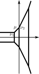
Figure 11: The tropical hypersurface $V(\operatorname{trop}(F))$.

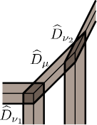
Figure 12: Regions $\widehat{D}_{\nu_{1}}$, $\widehat{D}_{\nu_{2}}$ and $\widehat{D}_{\mu}$.

The set $A_{\nu_{1}}$ defined in (2.2) is given by $\{(0,2),(1,1),(0,1)\}$. We set

$$\tilde{x}_{1}:=q^{2}x_{1}x_{2}/x_{2}^{2}=q^{2}x_{1}x_{2}^{-1},\qquad\tilde{x}_{2}:=qx_{2}/x_{2}^{2}=qx_{2}^{-1},$$

$$\widetilde{X}_{1}:=(2+X_{1}+X_{2})-(2X_{2})=2+X_{1}-X_{2},\qquad\widetilde{X}_{2}:=(1+X_{2})-2X_{2}=1-X_{2}.$$

Then the sets of functions $(\tilde{x}_{1},\tilde{x}_{2})$ and $(\widetilde{X}_{1},\widetilde{X}_{2})$ form standard coordinates on $O_{\{0\}}({\mathbb{C}})$ and $O_{\{0\}}({\mathbb{T}})$ with respect to $\nu_{1}$ defined in Section 2.3. Similarly, we have $A_{\nu_{2}}=\{(0,2),(1,1),(2,1)\}$ and we set

$$\tilde{x}_{3}:=q^{2}x_{1}^{2}x_{2}/x_{2}^{2}=q^{2}x_{1}^{2}x_{2}^{-1},\qquad\widetilde{X}_{3}:=(2+2X_{1}+X_{2})-(2X_{2})=2+2X_{1}-X_{2},$$

so that the sets of functions $(\tilde{x}_{1},\tilde{x}_{3})$ and $(\widetilde{X}_{1},\widetilde{X}_{3})$ form standard coordinates on $O_{\{0\}}({\mathbb{C}})$ and $O_{\{0\}}({\mathbb{T}})$ with respect to $\nu_{2}$. In addition, we have $A_{\mu}=\{(0,2),(1,1)\}$. Hence, the sets of functions $(\tilde{x}_{1},\tilde{x}_{2})$, $(\widetilde{X}_{1},\widetilde{X}_{2})$ and $(\tilde{x}_{1},\tilde{x}_{3})$, $(\widetilde{X}_{1},\widetilde{X}_{3})$ also form standard coordinates with respect to $\mu$. Let $W_{R}$ be the tropical localization defined in Definition 3.1 and $\phi\colon\operatorname{Log}_{R}(W_{R})\to V(\operatorname{trop}(F))$ be a map satisfying the condition $(\ast)$ in Proposition 4.1. Here, we set the map $\phi$ so that the restriction of $\phi$ to $\operatorname{Log}_{R}(W_{R})\cap\widehat{D}_{\rho}$ gives a bijection to $\rho$ for any edge $\rho\in P_{\{0\}}$. The manifold $W_{R}$, the map $\phi$ and the monodromy transformation $\psi\colon W_{R}\to W_{R}$ on each region are listed in Table 1.

Table 1: Monodromy transformation $\psi$ on each region.

region	$D_{\nu_{1}}$	$D_{\nu_{2}}$	$D_{\mu}$
standard coordinate	$(\tilde{x}_{1},\tilde{x}_{2})$	$(\tilde{x}_{1},\tilde{x}_{3})$	$(\tilde{x}_{1},\tilde{x}_{2})$ or $(\tilde{x}_{1},\tilde{x}_{3})$ 2pt3pt
tropical localization $W_{R}$	$1$-dimensional tropically localized hyperplane in $(\tilde{x}_{1},\tilde{x}_{2})$	$1$-dimensional tropically localized hyperplane in $(\tilde{x}_{1},\tilde{x}_{3})$	$1$-dimensional cylinder in $\tilde{x}_{2}$ or $\tilde{x}_{3}$ 3pt
map $\phi$	constant map to $\nu_{1}$	constant map to $\nu_{2}$	bijection to $\mu$ 3pt
monodromy $\psi$	identity map	identity map	Dehn twist2pt

Since $\widetilde{X}_{1}(\nu_{1})=\widetilde{X}_{2}(\nu_{1})=0$ and $\widetilde{X}_{1}(\nu_{2})=\widetilde{X}_{3}(\nu_{2})=0$, we can see from Theorem 4.5 that the restrictions of $\psi$ to $D_{\nu_{1}}$ and $D_{\nu_{2}}$ are identity maps. On $D_{\mu}$, if we use $(\tilde{x}_{1},\tilde{x}_{2})$ as a coordinate system, we have $\widetilde{X}_{1}\equiv 0$ on $\mu$ and $\widetilde{X}_{2}(\nu_{1})=0,\widetilde{X}_{2}(\nu_{2})=-1$. Then we can also see from Theorem 4.5 that the restriction of $\psi$ to $D_{\mu}$ coincides with the Dehn twist in the component of the cylinder in $\tilde{x}_{2}$.

6.2 Example in dimension 2

Consider the polynomial $G(x_{1},x_{2},x_{3})=t^{-1}+x_{1}+x_{2}+x_{3}+x_{1}^{-1}x_{2}^{-1}x_{3}^{-1}$. Then we have

$$g_{q}(x_{1},x_{2},x_{3})=q+x_{1}+x_{2}+x_{3}+x_{1}^{-1}x_{2}^{-1}x_{3}^{-1},$$

$$\operatorname{trop}(G)(X_{1},X_{2},X_{3})=\max\{1,X_{1},X_{2},X_{3},-X_{1}-X_{2}-X_{3}\}.$$

The tropical hypersurface $V(\operatorname{trop}(G))$ is shown in Fig. 14. Let $\rho$ denote the $2$-cell of $V(\operatorname{trop}(G))$ contained in $X_{1}=1$ and $\nu_{1}$, $\nu_{2}$, $\nu_{3}$, $\mu_{1}$, $\mu_{2}$, $\mu_{3}$ denote faces of $\rho$ as shown in Fig. 14 ($\rho$ denotes the $2$-cell colored in light gray). Fig. 14 shows the intersections of the hyperplane $X_{1}=1$ and regions $\widehat{D}_{\nu_{i}}$, $\widehat{D}_{\mu_{i}}$ $(i=1,2,3)$ and $\widehat{D}_{\rho}$ defined in Definition 3.3.

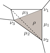
Figure 13: The tropical hypersurface $V(\operatorname{trop}(G))$.

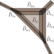
Figure 14: The intersections of the hyperplane $X_{1}=1$ and regions $\widehat{D}_{\nu_{i}}$, $\widehat{D}_{\mu_{i}}$, $\widehat{D}_{\rho}$.

The set $A_{\nu_{1}}$ is given by $\{(0,0,0),(1,0,0),(0,1,0),(0,0,1)\}$. We set $\tilde{x}_{i}:=x_{i}/q=q^{-1}x_{i}$ and $\widetilde{X}_{i}:=-1+X_{i}$ for $i=1,2,3$. Then the sets of functions $(\tilde{x}_{1},\tilde{x}_{2},\tilde{x}_{3})$ and $(\widetilde{X}_{1},\widetilde{X}_{2},\widetilde{X}_{3})$ form standard coordinates with respect to $\nu_{1}$ on $O_{\{0\}}({\mathbb{C}})$ and $O_{\{0\}}({\mathbb{T}})$. On the other hand, we have $A_{\mu_{1}}=\{(0,0,0),(1,0,0),(0,1,0)\}$, $A_{\mu_{3}}=\{(0,0,0),(1,0,0),(0,0,1)\}$ and $A_{\rho}=\{(0,0,0),(1,0,0)\}$. Hence, the sets of functions $(\tilde{x}_{1},\tilde{x}_{2},\tilde{x}_{3})$ and $(\widetilde{X}_{1},\widetilde{X}_{2},\widetilde{X}_{3})$ also form standard coordinates with respect to $\mu_{1}$, $\mu_{3}$ and $\rho$.

1. Tropical localization $W_{R}$ coincides with the following:

   1. On $D_{\nu_{1}}\colon$ the $2$-dimensional tropically localized hyperplane in $(\tilde{x}_{1},\tilde{x}_{2},\tilde{x}_{3})$.

   2. On $D_{\mu_{1}}\colon$ the direct product of the $1$-dimensional tropically localized hyperplane in $(\tilde{x}_{1},\tilde{x}_{2})$ and the $1$-dimensional cylinder in $\tilde{x}_{3}$.

   3. On $D_{\mu_{3}}\colon$ the direct product of the $1$-dimensional tropically localized hyperplane in $(\tilde{x}_{1},\tilde{x}_{3})$ and the $1$-dimensional cylinder in $\tilde{x}_{2}$.

   4. On $D_{\rho}\colon$ the direct product of $1$-dimensional cylinders in $\tilde{x}_{2}$ and $\tilde{x}_{3}$.

2. Let $\phi\colon\operatorname{Log}_{R}(W_{R})\to V(\operatorname{trop}(G))$ be a map satisfying the condition $(\ast)$ in Proposition 4.1. We set the map $\phi$ so that the restriction of $\phi$ to $\widehat{D}_{\rho^{\prime}}$ gives a surjection to $\rho^{\prime}$ for any cell $\rho^{\prime}\in P$.

3. Monodromy transformation $\psi$ is given as follows:

   1. On $D_{\nu_{1}}\colon$ the identity map.

   2. On $D_{\mu_{1}}\colon$ the map which is identical in the component of the $1$-dimensional tropically localized hyperplane in $(\tilde{x}_{1},\tilde{x}_{2})$ and coincides with the composition of four times of the Dehn twists in the component of the cylinder in $\tilde{x}_{3}$.

   3. On $D_{\mu_{3}}\colon$ the map which is identical in the component of the $1$-dimensional tropically localized hyperplane in $(\tilde{x}_{1},\tilde{x}_{3})$ and coincides with the composition of four times of the Dehn twists in the component of the cylinder in $\tilde{x}_{2}$.

   4. On $D_{\rho}\colon$ the map which coincides with the composition of four times of the Dehn twists in both components of the cylinders in $\tilde{x}_{2}$ and $\tilde{x}_{3}$.

   Since the restriction of the map $\phi$ to $\widehat{D}_{\nu_{1}}$ is the constant map to $\nu_{1}$ and $\widetilde{X}_{i}(\nu_{1})=0$ for $i=1,2,3$, it follows from Theorem 4.5 that the restriction of $\psi$ to $D_{\nu_{1}}$ coincides with the identity map. Since the restriction of the map $\phi$ to $D_{\mu_{1}}$ is a surjection to $\mu_{1}$ and $\widetilde{X}_{3}(\nu_{1})=0,\widetilde{X}_{3}(\nu_{2})=-4$, we can see from Theorem 4.5 that the restriction of $\psi$ to $D_{\mu_{1}}$ coincides with the composition of four times of the Dehn twists in the component of the cylinder in $\tilde{x}_{3}$. Similarly, it turns out that the restriction of $\psi$ to $D_{\mu_{3}}$ coincides with the composition of four times of the Dehn twists in the component of the cylinder in $\tilde{x}_{2}$. On $D_{\rho}$, we can also see from Theorem 4.5 that the map $\psi$ coincides with the composition of four times of the Dehn twists in both components of the cylinders in $\tilde{x}_{2}$ and $\tilde{x}_{3}$.

7 Relation to Zharkov’s work

Definition 7.1.

A convex lattice polytope $\Delta\subset M_{\mathbb{R}}$ is smooth if for each vertex $v$ of $\Delta$, there exists a ${\mathbb{Z}}$-basis $z_{1},\dots,z_{n+1}$ of $M$ such that ${\mathbb{R}}^{\geq 0}(\Delta-v)={\mathbb{R}}^{\geq 0}z_{1}+\cdots+{\mathbb{R}}^{\geq 0}z_{n+1}$.

Definition 7.2.

Let $\Delta\subset M_{\mathbb{R}}$ be a convex lattice polytope. We define the polar polytope $\Delta^{\ast}\subset N_{\mathbb{R}}$ of $\Delta$ by

$$\Delta^{\ast}:=\{n\in N_{\mathbb{R}}\,|\,\langle m,n\rangle\geq-1\ \mathrm{for\ all\ }m\in\Delta\}.$$

The convex lattice polytope $\Delta$ is called reflexive if it contains the origin $0\in M$ as its interior point and the polar polytope $\Delta^{\ast}$ is also a lattice polytope in $N_{\mathbb{R}}$.

Let $\Delta$ be a smooth and reflexive polytope in $M_{\mathbb{R}}$ and $B$ be a subset of $\Delta\cap M$ containing $0$ and all vertices of $\Delta$. Let further $T$ be a coherent triangulation of $(\Delta,B)$. We assume that $T$ is central, i.e., every maximal-dimensional simplex in $T$ has the origin $0\in M$ as it’s vertex. Let $\lambda\colon B\to{\mathbb{Z}}$ be an integral vector which is in the interior of the secondary cone (see [3, Chapter 7, Definition 1.4]) corresponding to $T$. We consider the function $f_{q}$ defined by

$$f_{q}(x):=q^{\lambda(0)}-\sum_{i\in B\setminus\{0\}}q^{\lambda(i)}x^{i}.$$

where $q\in S_{R}^{1}:=\{z\in{\mathbb{C}}\,|\,|z|=R\}$ for a sufficiently large $R\in{\mathbb{R}}^{>0}$. Let $X_{\Delta}$ be the toric manifold whose moment polytope is $\Delta$ and $V_{q}$ be the hypersurface in $X_{\Delta}$ defined by $f_{q}$. In this setting, Zharkov constructed the monodromy transformation of $\{V_{q}\}_{q\in S_{R}^{1}}$ as follows:

1. Let $\mu_{R}\colon X_{\Delta}\to\Delta$ be the weighted moment map defined by

   $$\mu_{R}(x):=\frac{\sum\limits_{m\in B}R^{\lambda(m)}|x^{m}|m}{\sum\limits_{m\in B}R^{\lambda(m)}|x^{m}|}.$$

   There exists a small neighborhood $U\subset\Delta$ of the origin $0\in\Delta$ such that $\mu_{R}(V_{q})\subset\Delta\setminus U$ for any $q\in S_{R}^{1}$. We set $\Delta^{\circ}:=\Delta\setminus U$. He constructs two families of regions $\{U_{\tau}\}_{\tau\in\partial T}$ and $\{\widetilde{U}_{\tau}\}_{\tau\in\partial T}$ in $\Delta^{\circ}$. For instance, in the case where

   $$f_{q}:=q-\big{(}x+xy+y+x^{-1}+x^{-1}y^{-1}+y^{-1}\big{)}$$ (7.1)

   and the triangulation $T$ is given as shown in Fig. 15, the families of regions $\{U_{\tau}\}_{\rho\in\partial T}$ and $\{\widetilde{U}_{\tau}\}_{\tau\in\partial T}$ are as shown in Figs. 17 and 17, respectively. $v_{i}$ and $w_{i}$ $(i=1,\dots,6)$ denote vertices and edges of $\Delta$ respectively as shown in Fig. 15. $U_{v_{i}}$, $\tilde{U}_{v_{i}}$ denote the regions colored in light gray and $U_{w_{i}}$, $\tilde{U}_{w_{i}}$ denote the regions colored in dark gray as shown in Figs. 17 and 17. We omit their construction here and refer the reader to [10, Section 3] about how to construct them.

   

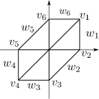
   Figure 15: The triangulation $T$ given by (7.1).

   

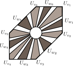
   Figure 16: Regions $\{U_{\tau}\}_{\tau\in\partial T}$.

   

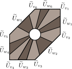
   Figure 17: Regions $\{\widetilde{U}_{\tau}\}_{\tau\in\partial T}$.

2. He sets bump functions $b_{m}\colon\Delta^{\circ}\to[0,1]\ (m\in B\setminus\{0\})$ so that the function $\tilde{f}_{q}\colon({\mathbb{C}}^{\ast})^{n+1}\to{\mathbb{C}}$ defined by

   $$\tilde{f}_{q}(x):=q^{\lambda(0)}-\sum_{m\in B\setminus\{0\}}(b_{m}\circ\mu_{R})(x)q^{\lambda(m)}x^{m}$$

   coincides with

   $$\begin{split}&q^{\lambda(0)}-\sum_{m\in\tau\cap B}q^{\lambda(m)}x^{m}\qquad\mathrm{on}\quad\mu_{R}^{-1}(U_{\tau})\cap({\mathbb{C}}^{\ast})^{n+1},\\ &q^{\lambda(0)}-\sum_{m\in\tau\cap B}(b_{m}\circ\mu_{R})(x)q^{\lambda(m)}x^{m}\qquad\mathrm{on}\quad\mu_{R}^{-1}(\widetilde{U}_{\tau})\cap({\mathbb{C}}^{\ast})^{n+1},\end{split}$$

   for any $\tau\in\partial T$. Let $W_{q}$ denote the submanifold in $X_{\Delta}$ defined by $\tilde{f}_{q}(x)=0$. We can see from the definition of the weighted moment map $\mu_{R}$ that if $\mu_{R}(x)\in\widetilde{U}_{\tau}$, the dominant part of $f_{q}$ at $x$ are $q^{\lambda(0)}-\sum\limits_{m\in\tau\cap B}q^{\lambda(m)}x^{m}$. Since orders of terms cut off by bump functions $\{b_{m}\}_{m\in B\setminus\{0\}}$ are lower, the submanifold $W_{q}$ is diffeomorphic to $V_{q}$.

3. He defines the family of subsets $\{\Delta_{\gamma}^{\vee}\subset N_{\mathbb{R}}\}_{\gamma\in[0,1]}$ by

   $$\Delta_{\gamma}^{\vee}:=\big{\{}n\in N_{\mathbb{R}}\,|\,{-}\langle m,n\rangle\geq\gamma(\lambda(m)-\lambda(0))\ \mathrm{for\ any\ vertex}\ m\ \mathrm{in}\ T\big{\}}.$$

   For any $\gamma>0$, the set $\Delta_{\gamma}^{\vee}$ is a convex polytope with a nonempty interior. The set $\Delta_{\gamma}^{\vee}$ in the case where $f_{q}$ is given by (7.1) is shown in Fig. 18.

   

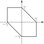
   Figure 18: The convex polytope $\Delta_{\gamma}^{\vee}$ in the case where $f_{q}$ is given by (7.1).

   The region surrounded by the center part of the tropical hypersurface coincides with

   $$\big{\{}n\in N_{\mathbb{R}}\,|\,\lambda(0)\geq\langle m,n\rangle+\lambda(m)\ \mathrm{for\ any\ vertex}\ m\ \mathrm{in}\ T\big{\}}.$$

   Hence when we set $\gamma=1$, the boundary of the convex polytope $\Delta_{\gamma=1}^{\vee}$ coincides with the center part of the tropical hypersurface. For each $k$-dimensional simplex $\tau\in\partial T$, we define an $(n-k)$-dimensional face $\tau^{\vee}$ of $\Delta_{\gamma}^{\vee}$ by

   $$\tau^{\vee}:=\big{\{}n\in\Delta_{\gamma}^{\vee}\,|\,{-}\langle n,m\rangle=\gamma(\lambda(m)-\lambda(0))\ \mathrm{for\ any\ vertex}\ m\ \mathrm{in}\ \tau\big{\}}.$$

   There is a bijective correspondence between simplices in $\partial T$ and faces of $\Delta_{\gamma}^{\vee}$ given by $\tau\leftrightarrow\tau^{\vee}$. Then he constructs a family of maps $\{v_{\gamma}\colon\Delta^{\circ}\to\partial\Delta_{\gamma}^{\vee}\}_{\gamma\in[0,1]}$ which depends on $\gamma$ smoothly and satisfies $v_{\gamma}(\widetilde{U}_{\tau})\subset\tau^{\vee}$ for any $\tau\in\partial T$.

4. Let $e_{i}:=(0,\dots,0,\overset{i}{\check{1}},0,\dots,0)\in M$ $(i=1,\dots,n+1)$ be the unit vector and $\psi_{i,\gamma}\colon X_{\Delta}\to{\mathbb{C}}$ $(i=1,\dots,n+1)$ be the function defined by

   $$\psi_{i,\gamma}:=\exp\big{(}2\pi\sqrt{-1}\langle(v_{\gamma}\circ\mu_{R})(x),e_{i}\rangle\big{)}.$$

   He defines a family of diffeomorphisms $\{D_{\gamma}\colon X_{\Delta}\to X_{\Delta}\}_{\gamma\in[0,1]}$ by

   $$(x_{1},\dots,x_{n+1})\to(\psi_{1,\gamma}x_{1},\dots,\psi_{n+1,\gamma}x_{n+1}).$$ (7.2)

   For any element $x\in W_{R}\cap\mu_{R}^{-1}(\widetilde{U}_{\tau})$, we have $\mu_{R}(D_{\gamma}(x))=\mu_{R}(x)\in\widetilde{U}_{\tau}$ and

   $$\tilde{f}_{q}(D_{\gamma}(x))=q^{\lambda(0)}-\sum_{m\in\tau\cap B}(b_{m}\circ\mu_{R})(x)q^{\lambda(m)}x^{m}\exp\big{(}2\pi\sqrt{-1}\langle v_{\gamma}(\mu_{R}(x)),m\rangle\big{)}$$

   $$\hphantom{\tilde{f}_{q}(D_{\gamma}(x))}{}=q^{\lambda(0)}-\sum_{m\in\tau\cap B}(b_{m}\circ\mu_{R})(x)q^{\lambda(m)}x^{m}\exp\big{(}{-}2\pi\sqrt{-1}\gamma(\lambda(m)-\lambda(0))\big{)}$$

   $$\hphantom{\tilde{f}_{q}(D_{\gamma}(x))}{}=\exp(2\pi\sqrt{-1}\gamma\lambda(0))\left\{R^{\lambda(0)}-\sum_{m\in\tau\cap B}(b_{m}\circ\mu_{R})(x)R^{\lambda(m)}{x}^{m}\right\}=0.$$

   Hence, the family of maps $\{D_{\gamma}\colon X_{\Delta}\to X_{\Delta}\}_{\gamma\in[0,1]}$ induces the monodromy transformation $\big{\{}D_{\gamma}\colon W_{R}\to W_{q=R\exp(2\pi\sqrt{-1}\gamma)}\big{\}}_{\gamma\in[0,1]}$.

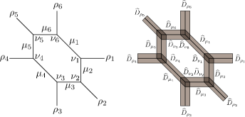
Figure 19: The tropical hypersurface and $\{\widehat{D}_{\mu}\}_{\mu}$ in the case where $f_{q}$ is given by (7.1).

As explained in (ii), Zharkov also localized the hypersurface $V_{q}$ to construct the monodromy transformation. He used the weighted moment map while we used the tropicalization. The regions $\{\widetilde{U}_{\tau}\}_{\tau}$ are similar to $\{\widehat{D}_{\mu}\}_{\mu}$ constructed in Definition 3.3. Moreover, terms which we cut off at each region are also the same. The tropical hypersurface and the family of regions $\{\widehat{D}_{\mu}\}_{\mu}$ are shown in Fig. 19 in the case where $f_{q}$ is given by (7.1). The region $\widetilde{U}_{v_{i}}$ corresponds to $\widehat{D}_{\mu_{i}}$ and $\widetilde{U}_{w_{i}}$ corresponds to $\widehat{D}_{\nu_{i}}$ $(i=1,\dots,6)$, respectively. For instance, on both $\widetilde{U}_{v_{2}}$ and $\widehat{D}_{\mu_{2}}$, the dominant terms are $q$ and $x$. On both $\widetilde{U}_{w_{1}}$ and $D_{\nu_{1}}$, the dominant terms are $q$, $x$, $xy$, and so on. Note that regions at which the term $q^{\lambda(0)}$ is not dominant in our construction are included in other regions in Zharkov’s construction. For instance, in the case $f_{q}$ is given by (7.1), the region corresponding to $\widehat{D}_{\rho_{i}}$ is included in $\widetilde{U}_{w_{i}}$ for $i=1,\dots,6$. This is the only major differences in the localization and the resulting manifolds $W_{q}$ are similar to each other.

His construction of the monodromy transformation is also similar to ours. We can construct the family of maps $\{v_{\gamma}\colon\Delta^{\circ}\to\partial\Delta_{\gamma}^{\vee}\}_{\gamma\in[0,1]}$ as follows. First, we construct $v_{\gamma=1}$ satisfying $v_{\gamma}(\widetilde{U}_{\rho})\subset\rho^{\vee}$ for any $\rho\in\partial T$. We set

$$S_{\gamma}\colon\ M_{{\mathbb{R}}}\to M_{{\mathbb{R}}},\qquad(X_{1},\dots,X_{n+1})\to(\gamma X_{1},\dots,\gamma X_{n+1}).$$

for each $\gamma\in[0,1]$. Then the map $v_{\gamma}:=S_{\gamma}\circ v_{\gamma=1}$ satisfies requested conditions. The map $\phi\colon\operatorname{Log}_{R}(W_{R})\to V(\operatorname{trop}(F))$ in Proposition 4.1 plays the same role as $v_{\gamma=1}$. Moreover, the monodromy transformation given by (4.2) in our construction coincides with (7.2). It can be said that our construction is a natural generalization of Zharkov’s construction.

Acknowledgements

The author would like to express his gratitude to Kazushi Ueda for encouragement and helpful advices. The author thanks to Tatsuki Kuwagaki for explaining the context of the paper [2]. The author also thanks the anonymous referees for reading this paper carefully and giving many helpful comments. This research is supported by the Program for Leading Graduate Schools, MEXT, Japan.

References

- [1] Abouzaid M., Homogeneous coordinate rings and mirror symmetry for toric varieties, Geom. Topol. 10 (2006), 1097–1157, math.SG/0511644.
- [2] Diemer C., Katzarkov L., Kerr G., Symplectomorphism group relations and degenerations of Landau–Ginzburg models, arXiv:1204.2233.
- [3] Gelfand I.M., Kapranov M.M., Zelevinsky A.V., Discriminants, resultants and multidimensional determinants, Modern Birkhäuser Classics, Birkhäuser Boston, Inc., Boston, MA, 2008.
- [4] Iwao S., Complex integration vs tropical integration, Lecture at The Mathematical Society of Japan Autum Meeting, 2010, available at http://mathsoc.jp/videos/2010shuuki.html.
- [5] Kajiwara T., Tropical toric varieties, Preprint, Tohoku University, 2007.
- [6] Kajiwara T., Tropical toric geometry, in Toric Topology, Contemp. Math., Vol. 460, Amer. Math. Soc., Providence, RI, 2008, 197–207.
- [7] Maclagan D., Sturmfels B., Introduction to tropical geometry, Graduate Studies in Mathematics, Vol. 161, Amer. Math. Soc., Providence, RI, 2015.
- [8] Mikhalkin G., Decomposition into pairs-of-pants for complex algebraic hypersurfaces, Topology 43 (2004), 1035–1065, math.GT/0205011.
- [9] Rullgård H., Polynomial amoebas and convexity, Preprint, Stockholm University, 2001, available at http://www2.math.su.se/reports/2001/8/2001-8.pdf.
- [10] Zharkov I., Torus fibrations of Calabi–Yau hypersurfaces in toric varieties, Duke Math. J. 101 (2000), 237–257, math.AG/9806091.