A distance limited sample of massive star forming cores from the RMS Survey

Abstract

We analyse C¹⁸O ($J=3-$2) data from a sample of 99 infrared-bright massive young stellar objects (MYSOs) and compact Hii regions that were identified as potential molecular-outflow sources in the Red MSX source (RMS) survey. We extract a distance limited (D $<$ 6 kpc) sample shown to be representative of star formation covering the transition between the source types. At the spatial resolution probed, Larson-like relationships are found for these cores, though the alternative explanation, that Larson’s relations arise where surface-density-limited samples are considered, is also consistent with our data. There are no significant differences found between source properties for the MYSOs and Hii regions, suggesting that the core properties are established prior to the formation of massive stars, which subsequently have little impact at the later evolutionary stages investigated. There is a strong correlation between dust-continuum and C¹⁸O-gas masses, supporting the interpretation that both trace the same material in these IR-bright sources. A clear linear relationship is seen between the independently established core masses and luminosities. The position of MYSOs and compact Hii regions in the mass-luminosity plane is consistent with the luminosity expected a cluster of protostars when using a $\sim$40 percent star-formation efficiency and indicates that they are at a similar evolutionary stage, near the end of the accretion phase.

1 Introduction

Massive stars ($>$ 8 M_⊙) are responsible for some of the most energetic phenomena in the Galaxy. They deposit large amounts of radiation, kinetic energy and enriched material into the interstellar medium (ISM) throughout their formation, main-sequence lifetimes and when they explode as supernovae. Massive young stellar objects (MYSOs) are the precursors to massive stars and are luminous ($\gtrsim$ 10³ L_⊙), mid-infrared point sources which have not yet begun to ionise their surroundings (Davies et al., 2010). The details of their early formation stages are difficult to probe observationally, due to their rare, clustered and embedded nature (Cesaroni et al., 2007). As a result, the processes of massive star formation are still relatively uncertain when compared to the well studied low-mass star-formation paradigm (Shu et al., 1987).

Theoretical modelling suggests that, during their formation, MYSOs with high accretion rates (10^-4 M_⊙ yr^-1) swell due to the mass influx. Consequently, they are deficient in ultraviolet (UV) photons until they begin contracting to a near-Main-Sequence configuration (Hosokawa & Omukai, 2009; Hosokawa et al., 2010); thus despite being very luminous, they are not initially ionising their surroundings. As the MYSOs contract towards the main sequence, they will then start to ionise the surrounding environment and form expanding Hii regions (Hoare & Franco, 2007). When the central stars reach the main sequence they generate copious amounts of UV photons, and so rapidly disrupt and destroy the natal cloud. Identifying MYSOs and very young Hii regions (very compact radio emitters, Lumsden et al., 2013) provides a sample of sources in which the natal environment will be less disrupted and therefore closer to their initial conditions, while simultaneously facilitating the investigation of feedback from the massive protostars known to be forming. The Red MSX Source (RMS) survey (Lumsden et al., 2013) is an ideal sample for this since it spans a wide range of luminosity and evolutionary stage. It also allows us to study how molecular gas properties vary as a function of both time and source luminosity.

This paper deals with the core properties of a sample of primarily northern RMS sources. These observations constitute the only RMS dataset so far in which the molecular-gas emission has been mapped, as opposed to obtaining single-pointing observations (cf. Urquhart et al., 2011). The primary goal of the observations was to study molecular outflows using single-dish observations of ¹²CO, ¹³CO and C¹⁸O ($J=3-$2) (discussed in a companion paper: Maud et al. 2015 submitted to MNRAS ). The aim of the C¹⁸O observations was to study the kinematical behaviour of the gas in the molecular core around the RMS sources. This allows us to determine outflow properties more reliably, but also permits us to study the cores separately. Single-dish C¹⁸O (3$-$2) is generally optically thin (Zhang & Gao, 2009) and excited in the denser regions when compared with lower-excitation transitions of CO (e.g. $J=1-$0). The $J=3-$2 emission is much less confused with line-of-sight emission than lower-excitation transitions, and a critical density for the transition of $>10^{4}$cm^-3 (with most emission expected to come from significantly higher densities - cf. Curtis & Richer 2011), makes it an ideal tracer of the core structures in star-forming regions.

Section 2 describes the source sample and observations undertaken, with Section 3 detailing the method used to calculate all source masses and their radii. Section 4 presents the basic results and the comparisons with previous data from the literature and the RMS survey itself. Section 5 discusses various relationships with source properties and in Section 6 we compare our results with a simple model to examine the star formation efficiency and protostellar evolution. A summary is given in Section 7.

2 Sample and Observations

2.1 Sample Selection

The sources were chosen from all MYSOs and Hii regions in the RMS survey that are located within a distance of $\sim$6 kpc, have luminosities $\gtrsim$ 3000 L_⊙, and are observable with the JCMT (declinations $-$25^∘ to $+$65^∘), with some additional right ascension constraints set by the observing dates. In addition, for the Hii regions, only those sources which appear compact in higher resolution mid-infrared images were selected. Finally although all of the sources with $L>10000$ L_⊙ were observed, only a random sample of the less luminous ones were included (see below). The original selection was made using the pre-2008 RMS catalogue and resulted in 99 target sources representative of the $\sim$200 MYSOs and compact Hii regions satisfying these criteria in the catalogue at that time. Since 2008, the RMS catalogue has evolved significantly as a result of subsequent observations. The updates to the RMS database have resulted in 10 of the initial sources now being assigned a kinematic distance beyond 6 kpc, where luminosities are only complete to $\sim$10⁴ L_⊙ (Mottram et al., 2011a); these are removed from the statistical sample (although masses are still calculated where possible). The luminosities for all sources have been recalculated using the most up-to-date source distances (Urquhart et al., 2012, 2014a) and multi-wavelength spectral energy distribution (SED) fits from Mottram et al. (2011b). As luminosities have changed the sample now extends to $\sim$1000 L_⊙, but is not complete below the original limits. Finally, there are now a total of $\sim$311 sources in the RMS catalogue that satisfy the original distance-limited criteria described above. Of these, we would expect about 50 Hii regions to be too extended ( based upon the RMS classifications), so that a complete distance-limited sample from the final catalogue would number approximately 260 sources.

The left panel of Figure 1 shows the luminosity distributions of the remaining 89 sources (dark grey) and of $\sim$450 objects in the RMS database (light grey) now matching the original criteria (but where L$>$1000 L_⊙ and source types are MYSO and both compact and extended Hii regions). The right panel shows the luminosities as a function of distance in the two sets of sources (filled and open circles, respectively). Both plots indicate that the range of luminosities and range of distances probed by the original observed sample is representative of all sources in the RMS database that satisfy the selection criteria. It is clear that the observed sample is incomplete in terms of relative numbers of sources at luminosities below $10^{4}$ L_⊙ (above which the RMS survey is now complete). This was always intended however, since our initial sampling aimed to have approximately equal numbers per logarithmic luminosity bin. Since all the analyses in this paper are essentially of ratios of observed quantities (e.g. Section 6, where luminosity is concerned), this numerical incompleteness is not a significant problem.

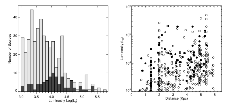
Figure 1: Left: Luminosity distribution of RMS sources now conforming to the original sample criteria (light grey bars) over-plotted with the luminosity distribution of the distance-limited set of observed sources (dark grey bars). The range of luminosities is well covered. Right: Comparison of the RMS distances and luminosities of the 89 sources in the distance-limited sample (filled circles) with the MYSOs and Hii regions now conforming to the original sample criteria (open circles) (see text for details). The sample covers the range of luminosity in the present population of $\sim$450 RMS sources that now match the original criteria. Note that sources at the same distance form part of known molecular complexes. Uncertainties are not indicated although are $\sim$ 30 percent for luminosity (Mottram et al., 2011b) and an illustrative value of 50 percent can be adopted for the distance.

2.2 Observations

All 99 sources were observed with the James Clerk Maxwell Telescope (JCMT) as part of projects M07AU08, M07BU16, M08AU19 and M08BU18 during 2007 and 2008. The 15-m dish yields a full-width half-maximum (FWHM) beam size of 15.3 arcsec at $\sim$329 GHz for the C¹⁸O (3-2) line. Throughout the observations, the typical median system temperatures were $T_{sys}$ $\sim$350$-$550 K. In a few cases, system temperatures reached as high as 900 K, reflected in a higher spectral noise level. The observations were taken with the Heterodyne Array Receiver Program (HARP) 16-pixel SSB SIS receiver (Buckle et al., 2009). The backend ACSIS correlator (Auto-Correlation Spectral Imaging System) was configured with an operational bandwidth of 250 MHz for the C¹⁸O transition. ¹³CO was simultaneously observed with C¹⁸O. The resulting velocity resolution was $\sim$0.06 km s^-1. The C¹⁸O and ¹³CO data were re-sampled to the velocity resolution of the ¹²CO data ($\sim$0.4 km s^-1) taken as part of the project, in order to match velocity bins for later outflow analysis and to improve the signal-to-noise ratio.

The maps were taken in raster-scan mode with continuous (on-the-fly) sampling and position switching to observe a ‘clean’ reference position at the end of each scan row. The maps range in size from 5 square arcminutes (5$\times$5 arcminutes) for those sources at distances $<$4 kpc, to 3 square arcminutes for those between 4 and 6 kpc. The pointing was checked with reference to a known bright molecular source prior to each source observation. Pointing accuracy is within $\sim$5 arcsec, as typically expected from JCMT observations. The majority of the baselines on each of the working receivers were flat, suitable for detecting the weak C¹⁸O emission. Some receivers did exhibit sinusoidal modulations and were flagged out from the final maps accordingly. Data reduction and display were undertaken with a custom pipeline which utilised the kappa, smurf, gaia and splat packages which are part of the starlink software maintained by the Joint Astronomy Centre (JAC). Linear baselines were fitted to the source spectra over emission-free channels and subtracted from the data cubes. The final C¹⁸O cubes used in all analyses were made with a 7-arcsec spatial pixel scale. The data, originally on the corrected antenna temperature scale ($T^{*}_{A}$; Kutner & Ulich, 1981) were converted to main-beam brightness temperature $T_{\rm mb}=T^{*}_{A}/\eta_{\rm mb}$, where $\eta_{\rm mb}=$ 0.66 as measured by JAC during the commissioning of HARP (Buckle et al., 2009) and via ongoing planet observations. Typical spectra noise levels are $\delta T_{\rm mb}\,\sim$ 0.8 K in a 0.4 km s^-1 bin.

3 Mass and Radius Determination

The column density and, hence, mass can be calculated if we assume LTE, and a constant $T_{\rm ex}$ and $\tau_{18}$ for each source, as outlined in Appendix A. The calculations rely on the accurate determination of $\int T_{\rm mb,18}\,d\upsilon$ over the source. The method used here is applicable to any molecular-line tracer and source geometry. It is the combined process of integration over velocity (i.e. creation of a moment zero map) followed by an aperture summation over the source area. The column density and therefore mass are calculated in each pixel via,

$$N({\rm C^{18}O})=5.0\,{\times}\,10^{12}\,\frac{{\rm exp}(16.74/T_{\rm ex})\,(T_{\rm ex}+0.93)}{{\rm exp}(-15.80/T_{\rm ex})}\,$$

$$\times\,\int T_{\rm mb,18}\,\frac{\tau_{18}}{[1-{\rm exp}(-\tau_{18})]}\,d\upsilon\;,$$ (1)

where $N({\rm C^{18}O})$ is in ${\rm cm^{-2}}$ and,

$$M_{\rm gas}=N({\rm C^{18}O})\bigg{[}\frac{{\rm H_{2}}}{\rm C^{18}O}\bigg{]}\mu_{\rm g}\,m(_{\rm H_{2}})\Omega\,D^{2}$$ (2)

where $\Omega$ is the solid angle of a pixel, $D$ is the distance to the source, (H₂/C¹⁸O) is the H₂ to C¹⁸O abundance ratio, where H₂/¹²CO = 10⁴ and ¹⁶O/¹⁸O is varied according to the relationship 58.8 $\times$ $D_{\rm gc}$(kpc) $+$ 37.1 (Wilson & Rood, 1994), and $\mu_{\rm g}$ = 1.36 is the total gas mass relative to H₂. A more detailed derivation of the column density and mass are given in Appendix A (note the constants to change units are not included in Equation 2 above).

The core velocity extent (integration range) is established via a direct investigation of the data cubes, channel by channel, specifically focusing on a 3-pixel-diameter region centred on the source location. The integration limits are set when all emission within this region drops below 3$\sigma_{T_{\rm mb}}$ (where $\sigma_{T_{\rm mb}}$ is the standard deviation from the line-free sections of the re-binned, $\sim$0.4-km s^-1 resolution spectra extracted at every pixel) while moving away from the source $V_{\rm LSR}$ in the directions of increasing and decreasing velocity. For the majority of sources the 3 $\sigma_{\rm MAP}$ contour level is directly traced in order to define a polygon aperture selecting which pixels to associate with the core, from the moment zero map after velocity integration (see Figure 2, centre, where the dotted contour and red contour are 3 $\sigma_{\rm MAP}$ and the aperture respectively). Some sources do not follow this aperture definition and are discussed below. All but five sources (the YSOs G023.6566$-$00.1273, G094.3228$-$00.1671, G108.4714$-$02.8176 and G125.7795$+$01.7285 and the Hii region G049.5531$-$00.3302) have strong C¹⁸O emission above the 3 $\sigma_{T_{\rm mb}}$ spectral-noise level. These 5 sources are not included in further analysis.

Figure 2 depicts the stages in the process for the source G078.1224$+$03.6320 (IRAS 20126$+$4104, a well studied MYSO). The left panel shows the average spectrum extracted in a 3-pixel diameter region centred on the source, the integration ranges indicated as dashed lines, and the centre panel is the map resulting from the integration in velocity. The mass calculated within the defined aperture tracing the 3 $\sigma_{\rm MAP}$ contour is $\sim$150 M_⊙, consistent with Shepherd et al. (2000, who obtained 104 M_⊙ from their C¹⁸O (1$-$0) interferometric observations) when using their Galactocentric distance of 8.1 kpc, a heliocentric source distance of 1.7 kpc, a calculated temperature of 26.1 K and without a correction made for $\tau_{18}$. As a final consistency check, we sum all the data within the aperture into a single spectrum and derive a mass from a Gaussian fit to this profile, as shown in the right panel. The result in this case is 149 $\pm$ 6 M_⊙, consistent with the previous estimate from velocity integration and aperture summation. Gaussian fitting of each individual spectrum (at each pixel) in the data cube is not used, however, as this would require a priori knowledge of the source size and emission region, which is only established after the integration stage.

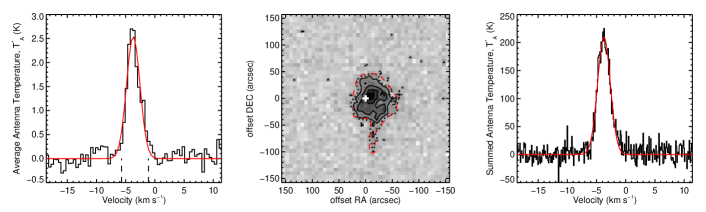
Figure 2: Left: C¹⁸O (3$-$2) line spectrum for G078.1224$+$03.6320, averaged within a 3-pixel diameter aperture centred on the RMS source location and smoothed to 0.4 km s^-1. The line profile is very close to that of a Gaussian, indicated by the red line. The long dashed lines show the velocity range within which the emission is integrated. Centre: Integrated intensity map of the C¹⁸O emission from G078.1224$+$03.6320 within the $-$5.7 to $-$1.1 km s^-1 velocity range. The dotted black line indicates the 3 $\sigma_{\rm MAP}$ contour while the solid lines are the contours at 90, 70, 50 and 30 percent of the peak emission value. The white cross indicates the RMS source location. Emission is summed within the polygon aperture, shown by the dashed red line tracing the 3 $\sigma_{\rm MAP}$ contour level. Right: The summed C¹⁸O spectrum extracted from the data cube within the polygon aperture defined from the integrated map (centre). The resultant spectrum has a high signal-to-noise ratio and is Gaussian in shape (red fitted line). The velocity resolution of the summed spectrum shown is $\sim$0.1 km ^-1 .

The source radii are calculated using the area within the defined apertures. An effective circular radius can simply be defined as

$$\theta_{\rm eff}=\sqrt{{area}/\pi}.$$

The deconvolved radius, assuming the JCMT has a Gaussian beam of diameter 15.3 arcseconds is

$$\theta_{decon}=1/2\left(\left[2\theta_{\rm eff}\right]^{2}-15.3^{2}\right)^{1/2}.$$

We tested for the influence that extended, low-surface-brightness emission might have on these values by clipping the data below 30 percent of the peak value rather than at the 3 $\sigma_{\rm MAP}$ contour. Although the deconvolved radii decrease, the masses also decrease by a similar factor when calculated within the same area. Virial-type analyses are therefore resilient against the choice of threshold. The mass and radius attributed to the cores are therefore consistent and refer to the same area as in previous similar studies (cf. Kauffmann et al., 2013).

Table 1 lists the sources, positions and important parameters extracted from the RMS survey online archive. In some cases, the types are listed as YSO/Hii where observable characteristics are consistent with both the MYSO and Hii-region classification and a definitive type cannot be ascertained (Lumsden et al., 2013). In some sources, multiple, close (a few arcsec separation), IR-bright targets have been identified (three targets would be listed as A, B, C in the online archive, for example). The YSO/Hii type is also used for these sources, if at least one MYSO and one Hii region is included. Individual MYSOs and Hii regions are inseparable at the resolution of the JCMT observations. Furthermore, where luminosities for each target have been estimated, the total for the source is listed in Table 1, highlighted with an asterisk (*).

Table 1: Source parameters for all objects in the sample, taken from the RMS survey online archive. The asterisk (*) highlights sources where multiple IR targets have been identified. Only a small portion of the data is provided here, the full table is available in the electronic supplementary information.

MSX Source Name	RA.	DEC.	Type	$V_{\rm LSR}$	Distance	Luminosity	IRAS source	Other
	(J2000)	(J2000)		(km s-1)	(kpc)	(L⊙)	(offset)	Associations
G010.8411$-$02.5919	18:19:12	$-$20:47:30	YSO	11.4	1.9	24000	18162$-$2048 (4$\arcsec$)	GGD27
G012.0260$-$00.0317	18:12:01	$-$18:31:55	YSO	110.6	11.1	32000	18090$-$1832 (3$\arcsec$)	…
G012.9090$-$00.2607	18:14:39	$-$17:52:02	YSO	35.8	2.4	32000	18117$-$1753 (11$\arcsec$)	W33A
G013.6562$-$00.5997	18:17:24	$-$17:22:14	YSO	48.0	4.1	14000	18144$-$1723 (2$\arcsec$)	…
G017.6380$+$00.1566	18:22:26	$-$13:30:12	YSO	22.5	2.2	100000	18196$-$1331 (11$\arcsec$)	…
G018.3412$+$01.7681	18:17:58	$-$12:07:24	YSO	32.8	2.9	22000	18151$-$1208 (16$\arcsec$)	…
G020.7438$-$00.0952	18:29:17	$-$10:52:21	Hii	59.5	11.8	32000	…	GRS G020.79$-$00.06
G020.7491$-$00.0898	18:29:16	$-$10:52:01	Hii	59.5	11.8	37000	…	GRS G020.79$-$00.06
G020.7617$-$00.0638*	18:29:12	$-$10:50:34	YSO/Hii	57.8	11.8	62000	…	GRS G020.79$-$00.06
G023.3891$+$00.1851	18:33:14	$-$08:23:57	YSO	75.4	4.5	24000	18305$-$0826 (6$\arcsec$)	GRS G023.64$+$00.14

Tables 2 and 3 list the derived source parameters, including temperature, optical depths, source radii and masses. In 4 of the 94 cores, the ¹³CO emission is optically thin $\tau_{13}\,<$1 and therefore cannot be used reliably to estimate the excitation temperature. For these sources, $T_{\rm ex}$ is obtained from the ¹²CO data obtained as part of this project using $\tau_{12}$. These sources are flagged with an asterisk (*) in Table 2. Although the ¹²CO data taken as part of this work is optically thick in all cores, these data are not used to establish the temperature of the C¹⁸O because: the $\tau_{12}$ =1 surface is further from the core than that of the ¹³CO which more closely matches the region of C¹⁸O emission; some of the ¹²CO spectra also exhibit very strong self absorption; and the ¹²CO temperature may be elevated in some sources by the influence of outflows.

Table 2: Optical depths, main-beam brightness temperatures, excitation temperatures and abundance ratios for all source with strong C¹⁸O emission. Sources with optically thin ¹³CO emission are flagged with an asterisk (*) to indicate that ${}^{12}{\rm CO}$ is used to calculate $T_{\rm ex}$. The full table is available in the electronic supplementary information.

MSX Source Name	$T_{\rm mb,13}$	$T_{\rm mb,18}$	$\tau_{13}$	$\tau_{18}$	$T_{\rm ex}$	Self Abs.	13CO/C18O	H2/C18O (104)
G010.8411$-$02.5919	20.29 $\pm$ 0.21	11.34$\pm$ 0.28	6.07 ${}^{+0.35}_{-0.33}$	0.81 ${}^{+0.05}_{-0.04}$	27.56 ${}^{+0.23}_{-0.23}$	yes	7.4	419.3
G012.0260$-$00.0317	7.78 $\pm$ 0.26	2.42 $\pm$ 0.34	2.37 ${}^{+0.72}_{-0.67}$	0.33 ${}^{+0.10}_{-0.09}$	15.21 ${}^{+1.37}_{-0.77}$	no	7.2	237.0
G012.9090$-$00.2607	13.26 $\pm$ 0.75	7.49 $\pm$ 0.18	6.15 ${}^{+0.89}_{-0.72}$	0.83 ${}^{+0.12}_{-0.10}$	20.24 ${}^{+0.82}_{-0.80}$	yes	7.4	395.8
G013.6562$-$00.5997	7.83 $\pm$ 0.30	3.33 $\pm$ 0.40	3.94 ${}^{+1.00}_{-0.86}$	0.54 ${}^{+0.13}_{-0.12}$	14.55 ${}^{+0.59}_{-0.44}$	yes	7.3	301.7
G017.6380$+$00.1566	14.22 $\pm$ 0.20	8.17$\pm$ 0.28	6.34 ${}^{+0.52}_{-0.48}$	0.85 ${}^{+0.07}_{-0.06}$	21.25 ${}^{+0.23}_{-0.23}$	no	7.4	413.4
G018.3412$+$01.7681	20.90 $\pm$ 0.24	7.07 $\pm$ 0.33	2.84 ${}^{+0.26}_{-0.26}$	0.38 ${}^{+0.04}_{-0.03}$	29.47 ${}^{+0.69}_{-0.58}$	no	7.4	378.1
G020.7438$-$00.0952	16.70$\pm$ 0.24	5.71 $\pm$ 0.26	2.85 ${}^{+0.27}_{-0.27}$	0.39 ${}^{+0.03}_{-0.04}$	24.87 ${}^{+0.61}_{-0.52}$	no	7.3	325.2
G020.7491$-$00.0898	16.70 $\pm$ 0.24	5.71$\pm$ 0.26	2.85 ${}^{+0.27}_{-0.27}$	0.39 ${}^{+0.03}_{-0.04}$	24.87 ${}^{+0.61}_{-0.52}$	no	7.3	325.2
G020.7617$-$00.0638	9.58$\pm$ 0.23	2.60 $\pm$ 0.29	1.94 ${}^{+0.49}_{-0.48}$	0.26 ${}^{+0.07}_{-0.06}$	18.02 ${}^{+1.68}_{-1.01}$	no	7.3	331.1
G023.3891$+$00.1851	6.32 $\pm$0.28	3.42 $\pm$ 0.22	5.67 ${}^{+1.06}_{-0.87}$	0.77 ${}^{+0.15}_{-0.12}$	12.71 ${}^{+0.35}_{-0.33}$	no	7.3	307.6

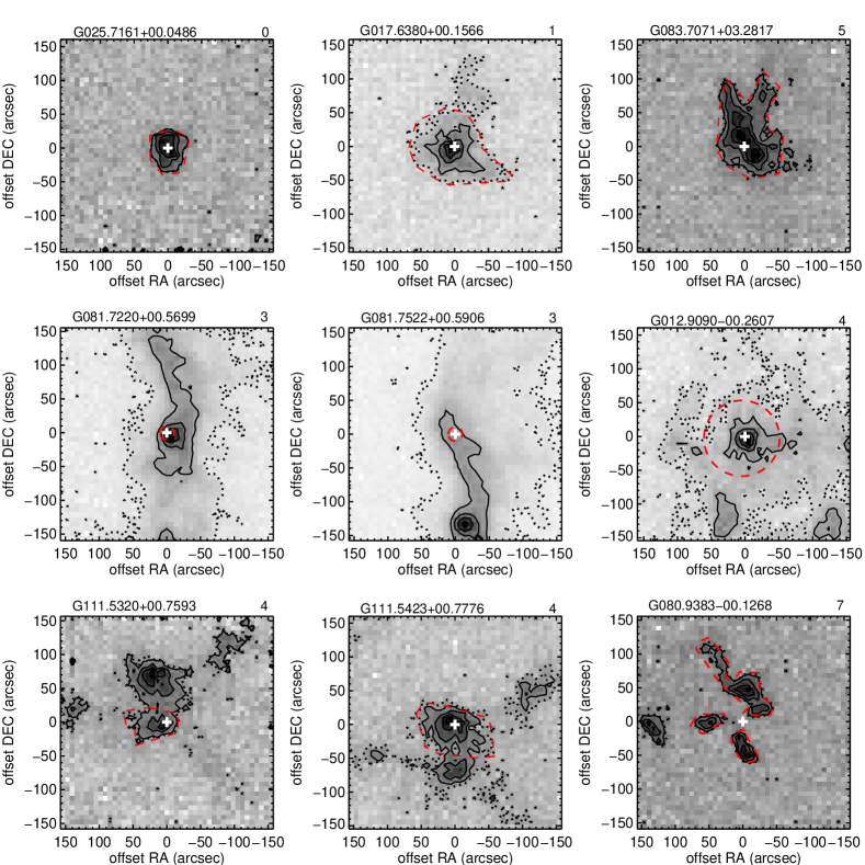
Figure 3: Integrated C¹⁸O (3$-$2) maps of sources with a range of mass flags. From left to right, top to bottom, are example sources indicating the various summation apertures for flags 0, 1, 5, 3, 4, and 7. The source name and corresponding flag is listed above the maps. Flag 3 is illustrated by two sources in the G081.7XXX region to exemplify the $\sim$3 pixel diameter summation aperture. For flag 4, there are 3 sources shown. G012.9090$-$00.2607 has a circular aperture with a radius set from the source peak to the closest edge of the 3$\sigma_{\rm MAP}$ noise level. The sources G111.5320$+$00.7593 and G111.5423$+$00.7776 are a split structure where emission is divided mid way between the sources. For G080.9383$-$00.1268 (flag 7), it is clear that the emission is not peaked on the source location of the Hii region. In all maps the dotted black line indicates the 3$\sigma_{\rm MAP}$ contour, while the solid contours are the emission at 90, 70, 50 and 30 percent of the peak. The white cross indicates the RMS source location and the summation aperture is indicated by the dashed red line. Flag 2 sources are not shown as they are indistinguishable from type 0 or 1 in the maps, while flag 6 sources are not shown as these can fall into any other flag category.

Table 3: Measured parameters for all sources. The masses are listed from the polygon aperture method and the Gaussian summation fitting where applicable. The full table is available in the electronic supplementary information.

MSX Source Name	Type	Spectral	Vel. Range	Map Noise	FWHM	Centroid	Aperture	Gaussian	Decon.	Flag
		Noise					Mass	Mass	Radius
		(K)	(km s-1)	(K km s-1)	(km s-1)	(km s-1)	(M⊙)	(M⊙)	(pc)
G010.8411$-$02.5919	YSO	0.8	( 9.9 , 14.6 )	1.4	1.9	12.2	465 $\pm$ 10	450 $\pm$ 12	0.47	1
G012.0260$-$00.0317	YSO	1.4	(110.4 ,112.1 )	1.5	3.2	110.9	269 $\pm$ 33	469 $\pm$ 92	0.53	0
G012.9090$-$00.2607	YSO	0.6	( 32.6 , 40.2 )	1.7	4.4	36.3	1065 $\pm$ 79	1104 $\pm$ 26	0.64	4
G013.6562$-$00.5997	YSO	1.4	( 46.4 , 48.9 )	1.6	3.1	47.8	108$\pm$ 12	144 $\pm$ 22	0.21	0
G017.6380$+$00.1566	YSO	0.6	( 19.9 , 25.9 )	1.2	2.6	22.3	616 $\pm$ 22	597 $\pm$ 19	0.61	1
G018.3412$+$01.7681	YSO	0.7	( 31.1 , 35.8 )	1.3	2.3	32.8	606 $\pm$ 12	614 $\pm$ 20	0.68	1
G020.7438$-$00.0952	Hii	1.0	( 60.0 , 60.8 )	0.8	3.3	59.1	594 $\pm$ 14	2450 $\pm$ 150	1.06	0
G020.7491$-$00.0898	Hii	0.8	( 56.1 , 62.1 )	1.8	3.8	58.8	6067 $\pm$ 147	6374 $\pm$ 380	2.23	0
G020.7617$-$00.0638	YSO/Hii	1.0	( 55.3 , 58.3 )	1.3	3.6	56.4	617 $\pm$ 56	892 $\pm$ 101	0.65	2
G023.3891$+$00.1851	YSO	0.8	( 73.8 , 76.7 )	1.0	2.0	75.3	358 $\pm$ 37	376 $\pm$ 30	0.49	0

Mass flags follow the scheme:
0 $-$ Masses calculated directly from within aperture tracing the 3 $\sigma_{\rm MAP}$ level.
1 $-$ Faint filamentary structures are not included in mass calculation and are outside the aperture. In extreme cases the aperture is more circular.
2 $-$ Highlights cores with multiple IR-bright sources within JCMT beam (Classically flag type 0 or 1).
3 $-$ Source mass estimated within a 3-pixel diameter aperture (slightly over 1 beam FWHM) aperture centred on the source due to the source being part of a complex filamentary cloud complex.
4 $-$ Complex/multiple source regions of significant emission. Masses are split where emission peaks are separated by more than 3 pixels or are circular with a radius set as the shortest distance between the RMS source location and the 3 $\sigma_{\rm MAP}$.
5 $-$ Two or more inseparable continuum cores very close within the aperture.
6 $-$ Luminosity estimates not from SED fitting.
7 $-$ Morphology suggesting that gas located at the source position has already been blown away or eroded.

Not all of our source maps show an ideal source distribution, such as the test source G078.1224$+$03.6320, Figure 2. Some include diffuse emission or joined targets, thus they have a different morphology and their mass apertures do not trace the 3$\sigma_{\rm MAP}$ contour directly. In Table 3 each source is given a mass flag according to its map morphology and aperture definition, as detailed in the table caption. These flags indicate whether the source masses are reliable estimates and are used in the analysis, or are considered unreliable, due to confusion or merging with other sources. Some sources are deemed to have unreliable masses where we are unable to define a mass aperture following the above outlined method, i.e. tracing the 3 $\sigma_{\rm MAP}$ contour level. Figure 3 presents an example source from each flag category, except flag types 2 and 6. The masses from sources with 0, 1 and 2 flags are used in the analysis fully as their mass apertures essentially follow the outlined method (see the Table 3 caption), although flag 4 sources are used with caution where indicated throughout the paper. Sources with the other mass flags are not used in the analysis as the masses are clear underestimates, the source emission is indistinguishable from other cores in the region or emission is not associated with the source itself ( see the Table 3 caption in correspondence with Figure 3 for the list of mass flags and differences in aperture definitions). Overall there are 61 (of 89 D $<$ 6 kpc) sources flagged as 0, 1 and 2 that are regarded as having good mass and luminosity estimates for the cores (70 when including flag 4 targets), these all have apertures closely following the 3$\sigma_{\rm MAP}$ contour, the remaining sources have different aperture definitions and are therefore not used in further analysis. The integrated images, polygon apertures and summed Gaussian spectra of all 99 sources (including sources with distance $>$ 6 kpc) are presented in Appendix B (available online). The sources with flags 0, 1, 2 and 4 for which we have derived masses are plotted in all figures henceforth (unless otherwise indicated).

4 Results

4.1 C¹⁸O Mass and Distance

Figure 4 shows that a wide range of masses are sampled at all distances in our sample, indicative of no distance dependent biases. Furthermore, there are no biases towards MYSOs and Hii regions independently and the two source types span the same mass and distance ranges. In general, the sources flagged as 4 also have masses well within the range of those identified as having reliable estimates. It is likely that the division of mass between sources in multi-core regions is reasonable in these cases. There are still a few flag 4 sources where the masses ($\gtrsim$1000 M_⊙) are likely to be overestimates due to the nature of the aperture definitions in these cases, and may include un-associated material with the core (see Appendix B).

All the cores are resolved at distances $<$6 kpc. However we cannot resolve sub-structures within the beam. It is likely that these cores will form stellar clusters containing lower-mass stars as well as the targeted massive protostar (see Bontemps et al., 2010, for an example of a relatively close region Cygnus X where substructure is clear). This is supported by the fact that flag 2 sources are indistinguishable from flag 0 and 1 sources in the C¹⁸O maps, although multiple infrared sources, with separations less than the JCMT beam, are identified in these cores. Clearly we are studying the properties of the natal cores of the associated star forming sites here rather than the reservoirs associated with individual stars.

Figure 4: Mass versus distance for all sources flagged as 0 and 1 (circles), 2 (squares) and 4 (triangles). The open symbols represent MYSOs and the filled ones are Hii regions. There is a wide range of masses probed for the different source types and flags located at distances $<$6 kpc. Note the error bars in the lower right represent a 50 percent uncertainty.

4.2 Comparison with Continuum Masses

We compared the C¹⁸O masses with those calculated from the 850 $\mu$m integrated fluxes from the SCUBA legacy survey (Di Francesco et al., 2008), BOLOCAM 1.1 mm integrated fluxes (Ginsburg et al., 2013) and other 1.2 mm observations (Beuther et al., 2002; Faúndez et al., 2004; Hill et al., 2005). The continuum fluxes have been used to calculate the masses traced by cool dust (Table 4) under the optically thin assumption via:

$${M}=\frac{{g}\,{S}_{\nu}\,{D}^{2}}{{\kappa_{\nu}}\,{B_{\nu}(T_{d})}}$$ (3)

where ${S}_{\nu}$ is the integrated source flux, ${g}$ is the gas-to-dust ratio = 100, ${B_{\nu}(T_{d})}$ is the Planck function for a black-body at a dust temperature $T_{\rm d}$ and ${D}$ is the distance to the source. ${\kappa}_{\nu}$ is the dust opacity coefficient, calculated via ${\kappa}_{\nu}$= ${\kappa}_{0}$ ($\nu/\nu_{0}$)^β, adopting ${\kappa}_{0}$ = 1.0 cm² g^-1 at 250 GHz (Ossenkopf & Henning, 1994) and $\beta$ = 2 (Beuther et al., 2002) and hence are 1.99 and 1.19 cm² g^-1 for SCUBA (850 $\mu$m) and BOLOCAM (1.1 mm), respectively. Assuming the gas and dust are in thermal equilibrium, the calculated C¹⁸O gas temperature for each source is used as the effective dust temperature. This is realistic given the densities of such cores ($>$10⁴ cm^-3, Fontani et al., 2012). Furthermore, the mean gas temperature for all sources is $\sim$23 K, close to typically assumed dust temperatures (e.g. Hill et al., 2005) and the kinetic temperatures calculated from ammonia observations for some of these sources (Urquhart et al., 2013). The fluxes listed in the literature are used directly and thus the continuum emission regions are unlikely to be exactly matched to the emission area of C¹⁸O and between the different continuum surveys.

Figure 5 shows that the 850 $\mu$m SCUBA, 1.1 mm BOLOCAM and various 1.2 mm observations correlate very well with the C¹⁸O masses (and each other). The BOLOCAM masses plotted here are derived using 80-arcsec aperture fluxes which better match the source sizes. The error bars represent a 50-percent uncertainty in the values. This is a reasonable estimate considering the calibration accuracy of the fluxes and the potential variations in dust/gas temperature, dust opacity, integration aperture selected and the C¹⁸O abundance ratio (e.g., a factor of $\sim$2.5 difference in mass can be caused by a change in assumed temperature between 10 and 20 K; Hill et al., 2005). There are a small number of outlier sources, G013.6562$-$00.5997, G025.4118$+$00.1052, G030.8185$+$00.2729 and G073.0633$+$01.7958 for which the dust-continuum masses are noticeably larger than the C¹⁸O masses (e.g. $>$ 5 times). Generally, the $\sim$order-of-magnitude scatter, may mean the choice of tracer is more important for individual objects, if not for the whole sample. However, all variations can be explained by a combination of mismatched aperture sizes between dust and gas studies, different noise levels and the aforementioned temperature and dust opacities.

Figure 5: Comparison of the C¹⁸O masses with the 850 $\mu$m SCUBA masses (circles), the 1.1 mm BOLOCAM masses (triangles) and 1.2 mm observations from various other surveys (diamonds). There is a dotted line representing equal masses and the dot-dashed line indicating the best bisector linear fit of the SCUBA and C¹⁸O masses. These follow each other very closely. Open symbols represent reliable C¹⁸O gas masses (flag 0, 1 and 2) and the filled symbols are for flag 4 sources (see text). The error bars in the lower right represent a 50 percent uncertainty.

The bisector line of best fit for SCUBA and C¹⁸O masses follows the 1:1 line closely in Figure 5. The slopes for SCUBA and BOLOCAM fits with the C¹⁸O masses are 1.0$\pm$0.12 and 1.14$\pm$0.12 respectively. The SCUBA observations appear to trace the same material for the majority of these cores. For the cores with largest gas masses the BOLOCAM masses are typically greater. However, this is likely to be due to the use of a constant aperture size for BOLOCAM fluxes and could include more faint, extended emission of the more massive regions in comparison to the polygon apertures chosen here. This is consistent with the association of C¹⁸O with denser gas as discussed below in Section 4.3.

Table 4: Continuum masses for a number of sources in the sample from BOLOCAM, SCUBA and other 1.2 mm observation. Masses are reasonably consistent between continuum observations. Dependent upon dust opacity, temperature and observable uncertainties a generous error estimate of $\sim$50 percent can be assumed (as Figure 5).

MSX Source Name	Type	BOLOCAM	SCUBA	1.2 mm
		(M⊙)	(M⊙)	(M⊙)
G010.8411$-$02.5919	YSO	…	139	210
G012.0260$-$00.0317	YSO	2188	3109	1853
G012.9090$-$00.2607	YSO	838	1167	1528
G013.6562$-$00.5997	YSO	1142	1385	1259
G017.6380$+$00.1566	YSO	358	374	…
G018.3412$+$01.7681	YSO	…	224	307
G020.7491$-$00.0898	Hii	4016	…	…
G020.7617$-$00.0638	YSO/Hii	1996	…	…
G023.3891$+$00.1851	YSO	1087	…	…
G023.6566$-$00.1273	YSO	584	…	…
G023.7097$+$00.1701	Hii	2569	…	2966
G025.4118$+$00.1052	YSO	886	1329	1446
G028.2007$-$00.0494	Hii	3099	4783	3693
G028.2875$-$00.3639	Hii	8234	9053	11894
G028.3046$-$00.3871	YSO	2537	…	1377
G030.1981$-$00.1691	YSO	…	372	…
G030.6877$-$00.0729	Hii	…	…	1956
G030.7206$-$00.0826	Hii	5666	…	2308
G030.8185$+$00.2729	YSO	432	440	415
G033.3891$+$00.1989	YSO	357	…	…
G037.5536$+$00.2008	YSO	4714	3552	3113
G043.9956$-$00.0111	YSO	408	597	…
G045.0711$+$00.1325	Hii	904	268	…
G048.9897$-$00.2992	YSO/Hii	1621	1830	…
G050.2213$-$00.6063	YSO	…	397	…
G053.9584$+$00.0317	Hii	332	…	…
G073.0633$+$01.7958	YSO	…	70	…
G075.7666$+$00.3424	YSO	138	88	…
G077.9550$+$00.0058	Hii	13	…	…
G077.9637$-$00.0075	Hii	9	…	…
G078.1224$+$03.6320	YSO	…	90	138
G078.8867$+$00.7087	YSO	391	611	…
G079.1272$+$02.2782	YSO	…	24	47
G079.8749$+$01.1821	Hii	54	…	…
G080.8624$+$00.3827	YSO	51	82	…
G080.8645$+$00.4197	Hii	89	137	…
G080.9383$-$00.1268	Hii	31	18	…
G081.7133$+$00.5589	Hii	…	367	…
G081.7220$+$00.5699	Hii	434	312	…
G081.7522$+$00.5906	YSO	260	272	…
G085.4102$+$00.0032	YSO/Hii	1448	2492	…
G094.6028$-$01.7966	YSO	…	845	…
G103.8744$+$01.8558	YSO	…	91	117
G105.5072$+$00.2294	YSO	480	…	…
G105.6270$+$00.3388	Hii	661	631	…
G109.0775$-$00.3524	YSO	404	179	…
G109.0974$-$00.3458	Hii	220	161	275
G109.8715$+$02.1156	YSO	88	112	…
G110.0931$-$00.0641	YSO	650	765	1013
G110.1082$+$00.0473	Hii	1008	1027	…
G111.2348$-$01.2385	YSO	301	235	391
G111.2552$-$00.7702	YSO	316	371	477
G111.5234$+$00.8004	YSO	135	109	…
G111.5320$+$00.7593	YSO	1033	1119	…
G111.5423$+$00.7776	Hii	1215	1167	…
G111.5671$+$00.7517	YSO	657	952	…
G111.5851$+$00.7976	YSO	…	12	…
G133.6945$+$01.2166	YSO/Hii	383	613	…
G133.7150$+$01.2155	YSO	…	794	…
G133.9476$+$01.0648	Hii	572	1148	…
G134.2792$+$00.8561	YSO	40	64	…
G136.3833$+$02.2666	YSO	109	164	…
G138.2957$+$01.5552	YSO	206	250	…
G139.9091$+$00.1969	YSO/Hii	…	163	…
G141.9996$+$01.8202	YSO	…	66	…
G192.5843$-$00.0417	Hii	293	291	220
G192.6005$-$00.0479	YSO	136	130	89
G196.4542$-$01.6777	YSO	…	279	…
G203.3166$+$02.0564	YSO	52	42	…
G207.2654$-$01.8080	YSO/Hii	…	172	…

Table 5 presents the results of a formal correlation analysis for the gas and dust masses for different source types and flags. Overall, the method used to calculate the C¹⁸O masses produces values that are directly proportional to continuum-based mass estimates. At the resolution of the JCMT, the C¹⁸O and SCUBA 850-$\mu$m emission effectively traces the same regions in the majority of the sources, and only in a few cases (where sensitivities are notably different between the sets of data) do the emission regions vary significantly. The BOLOCAM masses calculated from 80-arcsec aperture fluxes also provide reasonable matches to the C¹⁸O gas masses but fixed apertures are not ideal for such sources. Continuum and C¹⁸O line emission clearly trace the same material for these IR-bright sources.

In previous studies, depletion of C¹⁸O is a known cause of reduced gas column density and, hence, reduced masses, for a range of cores (e.g. Caselli et al., 1999; Fontani et al., 2012; Yıldız et al., 2012). Table 6 from Bergin et al. (1995) shows that the amount of CO in the gas phase varies by a factor of $\sim$2 between dust temperatures of 20 to 24 K, which closely matches the calculated temperatures of some sources in this work. López-Sepulcre et al. (2010) also discuss how their gas masses are on average lower than those calculated from dust emission although they suggest an incorrect abundance ratio can account for this. Clearly adopting a different H₂/¹²CO ratio other than 10⁴, by a factor of 2, i.e. setting H₂/¹²CO $\sim$ 2$\times$10⁴ will already alleviate any discrepancy in dust and gas masses. Factor of 2 offsets have been found in massive, pre-stellar cores (Fontani et al., 2006) and attributed to depletion. Here the reasonable correspondence of the gas and dust masses indicates that depletion of CO is not significant in the majority of these IR-bright RMS sources, especially when contrasted with the IR-dark cores in the aforementioned studies. Depletion could cause some of the scatter we see, however the already discussed variations in apertures size, dust opacity and temperature for example, can also explain this.

Table 5: Table of Spearman rank correlation values comparing dust and gas masses. The significance of a given $\rho$ value depends on the sample size (see Table A2.5, of Wall & Jenkins 2003, from which we have also adopted the quoted P-values). P-values of 0.05, 0.002 and $<$0.001 represent the $\sim$2, 3 and $>$3$\sigma$ confidence levels.

Correlation	Size	$\rho$	P-value
SCUBA
All (flag 0$+$1)	39	0.60	$<$0.001
All (flag 0, 1, 2$+$4)	46	0.60	$<$0.001
YSO (flag 0, 1, 2$+$4)	32	0.53	0.001
Hii (flag 0, 1, 2$+$4)	14	0.64	0.01
BOLOCAM
All (flag 0$+$1)	33	0.50	0.002
All (flag 0, 1, 2$+$4)	39	0.58	$<$0.001
YSO (flag 0, 1, 2$+$4)	23	0.22	0.3
Hii (flag 0, 1, 2$+$4)	16	0.86	$<$0.001

Finally, we stress that the masses calculated from the C¹⁸O emission are homogeneous in their determination and definitively associated with only the targeted cores, given that they have a single velocity component. Kauffmann et al. (2013) for example, include only cores where single Gaussian components are found to avoid the arbitrary division of continuum masses between velocity components. These C¹⁸O observations therefore provide an ideal way to study the core mass and its relationship to other observables.

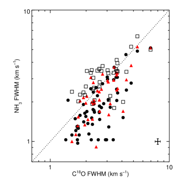
Figure 6: Comparison of the C¹⁸O linewidths with NH₃ (1,1) (filled circles), NH₃ (2,2) (red triangles), NH₃ (3,3) (squares) from Urquhart et al. (2011).The dotted line is the 1:1 line and is between the NH₃ (2,2) and NH₃ (3,3)transition. An average error of $\sim$ 5 percent from the fitting procedure is indicated.

4.3 Comparison with Other Linewidths

Previous observations of molecular gas, both in our own and other galaxies, have led to differences in derived properties depending on the species involved, and in particular when CO is compared to tracers of dense molecular gas (e.g. the discussion in Krumholz & Thompson 2007). We have compared our C¹⁸O linewidths ( measured using integrated spectra extracted from within the mass aperture regions, see Figure 2 and Appendix B) with those from NH₃ data from the single-dish observations of Urquhart et al. (2011) in Figure 6. The increase in linewidth with excitation energy in NH₃ is already well reported in similar types of sources (e.g. Longmore et al., 2007; Wienen et al., 2012), and is generally interpreted as due to the hotter gas being nearer the central exciting source, and with a smaller beam filling factor in the NH₃ observations (e.g. Urquhart et al., 2011). The widths are primarily driven by motions within the gas rather than temperature broadening, which would give far smaller values. Our data show that the C¹⁸O $J=3-2$ linewidths are consistent, in magnitude, with values between the NH₃(2,2) and NH₃(3,3) linewidths. The optically thin C¹⁸O 3–2 transition is tracing similar density ($\sim$ 10⁴ cm^-3) core material as the ammonia line, but should trace cooler gas than both NH₃(2,2) and NH₃(3,3), since the rotational energy levels (in temperature units) of the CO $J=3-2$ line ($\sim$33 K) and NH₃(1,1) ($\sim$23 K) are actually better matched (cf. NH₃(2,2) $\sim$ 65 K and NH₃(3,3) $\sim$ 125 K). This suggests that the CO ladder is actually thermalised to a higher $J$ level, and that the kinematics of the $J=3-2$ transition in our sources are actually representative of that warmer gas as well. We also compared the line centre velocities of the NH₃ and C¹⁸O, and found they agreed well, with no deviation larger than the typical spread in the various NH₃ linewidths shown in Figure 6. Again, this demonstrates that both these tracers are sampling similar gas properties and volumes.

We also compared the $J=3-2$ C¹⁸O and ¹³CO linewidths, with the latter larger by at least 10 percent. The largest differences are seen for those objects where the line opacity for ¹³CO is largest, so this is generally caused by the opacity of the CO lines rather than the fact that the ¹³CO line also traces outflow material. A similar trend towards increasing linewidth with increasing line opacity is also seen when comparing the C¹⁸O $J=3-2$ data with our previous lower $J$ transition data used in deriving kinematic distances (e.g. Urquhart et al., 2008). Indeed other similar surveys have commented on the difference in CO linewidth for the low lying isotopologues (e.g. Ao et al., 2004; Du & Yang, 2008; Wienen et al., 2012). The key message here is that different tracers may be more suitable in different circumstances. For example, the $J=3-2$ C¹⁸O studied here is clearly a good tracer of kinematics in reasonably dense clumps/cores, whereas $J=1-0$ ¹³CO is more suitable for probing the diffuse cool gas that delineates molecular clouds as a whole. This also indicates why the $J=1-0$ observations are a good tracer of gas in other galaxies, since the bulk of the mass will tend to be in the more diffuse molecular clouds. Notably the same may not be true in the dense environments found in extreme star forming galaxies (Harris et al., 2010).

The mean FWHM values for MYSOs and Hii regions are $\sim$ 2.6$\pm$0.1 and $\sim$3.1$\pm$0.2 km s^-1 respectively, where the uncertainties are the standard errors (including all sources where D $<$ 6 kpc and C¹⁸O is detected). The slightly larger FWHM for Hii regions might be interpreted as an evolutionary trend, where linewidths increase as the source has a greater impact upon its surroundings. However, such an interpretation is incorrect. As Urquhart et al. (2011) note, any such trend is artificial and caused by the luminosity-FWHM relationship due to the different luminosity functions for MYSOs and fully developed Hii regions (see Mottram et al., 2011b). Furthermore, the Hii regions here, as explicitly noted in Section 2, were selected to be compact and therefore should be at a similar evolutionary stage to the MYSOs. Figure 7 shows the relationship between the source luminosity and FWHM. Evidently, the Hii regions have a greater proportion of sources at luminosities $>$ 10⁴ L_⊙ (and correspondingly larger linewidths) which explains the slight offset of mean FWHM values reported. The Spearman rank correlation coefficient is 0.45 at $<$0.01 significance level, interpreted as a strong correlation for the 61 sources (with mass flags 0, 1 and 2). The relationship does hint at the most luminous sources providing more feedback and turbulence to the cores, possibly by driving more powerful outflows. This is examined further in Maud et al 2015 (submitted to MNRAS).

It is worth noting that some sources (30, 32-including those where D$>$6 kpc) show evidence of regular velocity gradients spatially across their cores. However, only a few of these appear to be aligned with, or perpendicular to the outflow direction. We stress that, given the resolution of the observations, it is difficult to ascertain the cause of the gradients in most cases, and whether the outflows are a major contributor.

Figure 7: Plot of luminosity versus C¹⁸O FWHM for all sources flagged as 0 and 1 (circles), 2 (squares) and 4 (triangles). The open symbols represent MYSOs and the filled ones are Hii regions respectively. A linear log-log relationship is seen between the parameters. The uncertainty from FWHM fitting is $\sim$ 5 percent whereas that for the luminosity is a representative 30 percent value (Mottram et al., 2011b).

In order to examine whether the CO lines profiles reveal the presence of infalling motions we derived the line asymmetry parameter using the definition of Mardones et al. (1997),

$$\delta\upsilon=\frac{\upsilon(thick)-\upsilon(thin)}{\Delta\upsilon(thin)}$$

where $\upsilon(thick)$ and $\upsilon(thin)$ are the velocities of the peak pixels measured from the spectra and $\Delta\upsilon(thin)$ is the FWHM of the thin tracer. Here C¹⁸O is the optically thin tracer (see Table 2), and the ¹²CO line is the optically thick one (also see Maud et al. 2015 submitted to MNRAS). The optically thin FWHM values of C¹⁸O are those given in Table 3. There is a spread of asymmetry values, ranging from $-$1 to +1.5 (where by the Mardones et al. 1997 criterion $|\delta\upsilon|>0.25$ indicates asymmetry). The results show that 23 sources have a red asymmetry, and 15 a blue asymmetry. At face value this can be taken as a lack of evidence for ongoing infall in our sample. However, we note that Fuller et al. (2005) also find a similar result in the profiles of the transitions they study which have similar excitation temperature and critical density, even though the same sources show strong blue asymmetry in, for example, HCO⁺ $J=1-0$. Our results appear to add evidence to their comment that it is the dense gas tracers that are best tracers of large scale infall. CO appears to be a poor tracer of infall for these cores, while HCO⁺ (4$-$3) is usually much better suited to these size scales (Klaassen & Wilson, 2007).

5 Analysis

5.1 Correlations within the Observables

We examined possible correlations amongst the observable parameters present in our sample, and within the wider information held as part of the RMS database. In addition we also considered combinations of these parameters. In particular we used the derived values from the C¹⁸O observations for radius, $T_{\rm ex}$, $\tau_{13}$, mass, line asymmetry and FWHM as well as combinations of these such as gas surface density, as discussed below. We took information on the luminosity, infrared colours and galactocentric radius, $R_{\rm gc}$ from the database (Lumsden et al., 2013), as well as a selection of the NH₃ properties from Urquhart et al. (2011). We used a Kendall correlation method for all of these comparisons. The Kendall method is generally held to be better in the presence of errors in the data (Wall & Jenkins, 2003), however typically both the Kendall and Spearman rank correlations lead to the same inferences. Here we choose the Kendall correlation since some parameters have ties in the data, where both pairs have the same ordinal.

The net result is that there are relatively few strong correlations, and many of those that are present are driven by the one obvious dominant relation, that between mass and radius. A partial correlation analysis confirms this. The only other strongly significant parameters are luminosity and FWHM. Table 6 shows the resultant correlations that have significance values $<0.002$.

The correlations that are not dependent on mass, luminosity, radius or FWHM can be summarised briefly as follows:

• The NH₃ kinetic temperatures, $T_{\rm kin}$, from Urquhart et al. (2011) agree reasonably with the $T_{\rm ex}$ values we derive here (See Appendix A).

• The kinetic temperatures are correlated with both infrared colour measures we use, $F_{W3}/F_{K}$ and $F_{8}/F_{K}$, with $T_{\rm ex}$ showing a slightly weaker correlation than $T_{\rm kin}$ (formally not significant at our threshold level for $F_{8}/F_{K}$).

• $\tau_{13}$ is anticorrelated with $R_{\rm gc}$.

The first of these essentially shows that the CO and NH₃ are tracing similar material, as we argued previously in Section 4.3. The second is curious since we might expect the redder objects to be more embedded and have lower kinetic temperatures rather than higher. It may indicate that these warmer sources simply have a more centrally concentrated mass distribution. This is not something that we can test with the spatial resolution of the current data. Finally the anticorrelation between $\tau_{13}$ and $R_{gc}$ may simply be a reflection of the observed anti-correlation between luminosity and $R_{\rm gc}$ found by Lumsden et al. (2013) in the full RMS sample (since $\tau_{13}$ is correlated with density, which is weakly correlated at the P$=0.025$ significance level with luminosity), even though no significant correlation between these variables is found in the much smaller sample here.

Table 6: Table of Kendall rank correlation values for various derived observables from both this paper and the wider RMS database. $R$ is the deconvolved source radius, $M$ the mass, $L$ the luminosity, $\Delta\upsilon$ the FWHM, $\rho$ the density, $\Sigma$ the gas surface density, $\tau_{13}$ the optical depth of ¹³CO, $R_{\rm gc}$ the Galactocentric radius, $t_{\rm ff}$ the free-fall time, $T_{\rm ex}(\rm CO)$ the excitation temperature of the ¹³CO, $T_{\rm kin}({\rm NH}_{3})$ the kinetic temperatures derived from NH₃ by Urquhart et al. (2011), $F_{8}/F_{K}$ the ratio of 8$\mu$m MSX flux with $K$ band flux as derived for Lumsden et al. (2013) and $F_{W3}/F_{K}$ the ratio of the WISE band 3 flux (approximately $10\mu$m) with $K$ band flux. The $-$ indicates data where there are ties so no well defined significance exists. The significance is the probability that the null hypothesis, i.e. there is no correlation, is correct.

Correlation	Sample Size	$\tau$	Significance
$R-M$	58	0.78	$<0.0001$
$R-\Delta\upsilon$	58	0.29	$0.002$
$R-L$	58	0.47	$<0.0001$
$M-\Delta\upsilon$	58	0.39	$<0.0001$
$M-L$	58	0.51	$<0.0001$
$\Delta\upsilon-\rho$	58	0.35	$0.0001$
$\Delta\upsilon-\Sigma$	58	0.35	$0.0001$
$\tau_{13}-\rho$	58	0.35	$0.0001$
$\tau_{13}-R_{\rm gc}$	58	$-0.37$	$<0.0001$
$\tau_{13}-\Sigma$	58	0.35	$0.0001$
$t_{\rm ff}-\Sigma$	58	$-0.42$	$<0.0001$
$T_{\rm ex}(CO)-T_{\rm kin}({\rm NH}_{3})$	41	0.52	-
$T_{\rm kin}({\rm NH}_{3})-F_{8}/F_{K}$	37	0.42	-
$T_{\rm kin}({\rm NH}_{3})-F_{W3}/F_{K}$	31	0.41	-
$\Sigma_{\rm SFR}=\Sigma/t_{\rm ff}$	58	0.49	$<0.0001$

Mass, luminosity, size of clump and FWHM are all positively correlated with each other (the luminosity-FWHM correlation has a significance level of only 0.003 however). These four collectively are what is expected from the scaling relationships of Larson (1981). Indeed, appropriate projections of the mass-luminosity-radius plane, for example, result in most data points being strongly clustered (i.e., there is a mass-radius-luminosity fundamental plane), though the luminosity component of this relationship is small, and the same is true for mass, FWHM and radius. The first of these can be understood, for example, as Larson’s third relation (mass-radius) but modified for the case of cores where a not insignificant fraction of the mass is now locked into stars (and hence not traced by the gas mass: cf. Section 6.1.2). The weak luminosity dependence of this mass-radius relation effectively compensates by directly tracing the mass already locked into stars. The strong correlation of mass and luminosity reflects the fact that these sources are of a similar evolutionary state, otherwise more scatter would be evident. Davies et al. (2011) shows that Hii regions can be of a similar age to massive protostars if the central source is itself more massive (i.e. more massive objects evolve more quickly towards the zero age main sequence). This conclusion is justified further in Section 6. It is notable that the FWHM and radius (Larson’s first relation) gives the weakest correlation, as shown in Table 6. We will discuss this and the other Larson relations in detail in the following sections, as well as comparing our results with those of Urquhart et al. (2014b) and Heyer et al. (2009). Heyer et al. (2009) used ¹³CO $J=1-0$ data from the Galactic Ring Survey (Jackson et al., 2006) to re-examine the underlying physical principles that lead to Larson’s scaling relations for molecular-cloud-sized structures and, hence, sampled much larger regions but with much lower surface densities. Urquhart et al. (2014b) analysed ATLASGAL sources (including those with RMS counterparts) and hence studied the continuum dust emission of similar regions to us.

Some of the properties that show no correlation are also worth mentioning. The line asymmetry parameter shows no correlation with any other properties, including the line opacity itself for example. There are no correlations between infrared colour and properties such as mass, or line asymmetry, where both red and blue asymmetric data show the same average colour, or between most of the CO properties (including opacity and column density) and infrared colour. The beamsize of our JCMT data are not dissimilar to many of the mid- and far-infrared data we use the infrared colours from. The natural explanation for the lack of correlation therefore is that there is substructure within the beam for both sets of data. In particular the CO data presented here traces cooler gas, whereas the infrared colours we have are predominantly a combination of hot and warm dust and extinction. The spatial scales of these components should differ considerably but we are unable to probe such detail. This also tallies with the discussion above regarding the actual correlation seen between $T_{\rm ex}$ or $T_{\rm kin}$ and colour.

5.2 Mass and Radius

Previous observations of molecular clouds/cores suggest a power-law scaling between mass and length scale (size, radius) of the form $m\propto r^{\gamma}$, where $\gamma\sim 2$ (e.g. Larson, 1981; Elmegreen & Falgarone, 1996; Kirk et al., 2013; Kauffmann et al., 2013). Their observations include different regions, associations (low- and high-mass stars) and observations using both molecular line tracers and continuum emission. Figure 8 shows the C¹⁸O masses plotted against deconvolved radius for our sample. The linear trend when including the flag 0, 1 and 2 sources follows the power law $m\propto r^{2.0\pm 0.1}$, where the uncertainty only accounts for the spread in the raw mass and radius values. Note, exchanging the deconvolved radii for the effective radii has a minimal effect and slightly steepens the slope to $m\propto r^{2.1\pm 0.1}$.

The ATLASGAL clumps associated with RMS sources investigated by Urquhart et al. (2014b) span a larger range of radii and mass, and follow a slightly shallower slope ($\gamma\sim 1.75\pm 0.04$) overall. There is a turnover in their data at higher masses, such that if we restrict the range to that of our sample a slightly steeper slope $\sim$1.9 would be recovered. However, the discrepancy in slopes can be attributed to the different methods in which mass and radius are calculated (we see that the slope changes when using effective radius). Urquhart et al. (2014b) find that the large scale clump properties follow the same trend from embedded maser sources to extended Hii regions (i.e. less to more evolved). They suggest the clump properties must therefore be set prior to the onset of star formation and that the subsequent evolution of massive protostars, and their feedback, does not effect the clumps overall. Note that the internal structures may still evolve (cf. the study of Kauffmann et al., 2010 which examined mass as a function of radius within single clumps, as opposed to the inter-clump comparisons given here). We basically find the same relations as Urquhart et al. (2014b) from the gas as opposed to dust. Heyer et al. (2009) find $\gamma\sim 2.17\pm 0.08$, again in reasonable agreement with the slope found here.

Where the Heyer data differs from the smaller clump/core sized regions studied here is in the offset of this relationship, which lies at lower masses in the Heyer et al sample. Fundamentally, both our sources and those of Urquhart et al. (2014b) are significantly more massive than the similar size regions in the sample of Heyer et al. (2009). It is worth reiterating that Heyer et al. used $J=1-$0 ¹³CO data. The comparison in Section 4.3 for our objects suggests such lines should be broader (due to opacity) than the $J=3-$2 C¹⁸O. Therefore, if anything, the true offset from a fair comparison with the Heyer et al. data may be even lower than suggested by the raw data. This is contrary to the spirit of the relation that Larson initially proposed.

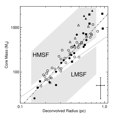
Figure 8: Core mass versus the deconvolved effective radius assuming spherical cores. Open and filled symbols are MYSOs and Hii regions respectively. The sources with 0 and 1 flags are represented by circles, flag 2 by squares and flag 4 sources by triangles. The general linear fit trend follows a power law ($\gamma$ = 2.0 $\pm$ 0.1) indicated by the dot-dashed line. The dotted line is that from Kauffmann & Pillai (2010) where massive star forming regions exceed a mass of 580 $R_{\rm pc}^{4/3}$. The upper and lower light grey boxed regions represent the high and low mass star forming regions presented in Kauffmann & Pillai (2010) after a reduction in mass by 1.5 to correct for the difference in dust opacity used. Note the larger, more massive ATLASGAL sources from Urquhart et al. (2014b) are predominantly located in the HMSF region where M$\gtrsim$1000 M_⊙ and R$\gtrsim$0.5 pc. A representative uncertainty of 50 percent in mass and an 10 percent illustrative uncertainty for the radius is indicated to the lower right.

Figure 9: Deconvolved source radius versus C¹⁸O FWHM for MYSOs (open) and Hii (filled) regions flagged as 0 and 1 (circles), 2 (squares) and 4 (triangles). The bisector fit best representing the data is shown as the dot-dashed line, and obeys FWHM $\propto r^{0.8\pm 0.5}$. An average uncertainty of 5 percent in FWHM and an illustrative 10 percent uncertainty in radius is indicated to the lower right.

5.3 FWHM-Mass and FWHM-Radius relationships

Figure 9 shows the log-log relationship between the C¹⁸O FWHM and deconvolved source radius. This comparison is analogous to the type-2, single tracer multi-core relationships presented in Goodman et al. (1998) where the FWHM is observed to decrease for smaller cores. The meaningful result of such a relationship is to examine whether the cores are virialised, where FWHM $\propto r^{0.5}$ is expected. The bisector fit best represents the data given the scatter (compared with ordinary least squares fitting, OLS, see Isobe et al., 1990), resulting in FWHM $\propto$r^0.8±0.5, roughly consistent with virialised cores. However, as already noted (Table 6), the significance of the correlation seen here is very weak (it is notably stronger for the data from Heyer et al. 2009). As with the results of the previous section, a noticeable offset exists in the relationship seen here and that of molecular cloud scales from the data of Heyer et al. (2009). The cores here exhibit much larger FWHM values. One possible cause for the weaker correlation and larger values is that on these scales feedback has a more significant impact compared to gravitational motions.

Larson (1981) noted a clear relationship between mass and velocity dispersion (linewidth) over many orders of magnitude in mass. Recent studies have confirmed this, though the tight relationship Larson found is less well reproduced. As the core masses are strongly related to the source radii, which in turn are weakly correlated to the linewidth, there is expected to be a link between mass and FWHMs for these sources. Figure 10 shows the correlation present between the mass and FWHM linewidths. A bisector best fit to the data indicates FWHM $\propto m^{0.37\pm 0.25}$, although the OLS fit is noticeably shallower, FWHM $\propto m^{0.18\pm 0.04}$, and closer to that found by Larson (1981) who fit by eye. The slopes are consistent given the uncertainties as a result of the scatter in the data. The Heyer et al. (2009) data give a similar slope, $\propto m^{0.20\pm 0.02}$, but again the relationship is offset, with smaller linewidths for molecular-cloud-sized regions at the same masses as in our sample.

Figure 10: Core mass versus the FWHM linewidth for MYSOs and Hii regions (open and filled symbols respectively). Flag 0 and 1, 2 and 4 are represented by circles, squares and triangles. The plotted dotted line is the OLS best fit with a similar slope (FWHM $\propto m^{0.18\pm 0.04}$) to the by-eye fit from Larson (1981). The bisector fit better represents the data given the scatter and has a steeper slope, $FWHM\propto m^{0.37\pm 0.25}$. The average uncertainty of 5 percent in FWHM and representative 50 percent uncertainty for the mass is shown to the bottom right.

5.4 Virial Mass and Gas Surface Density

Star formation has already occurred in these cores as they harbour at least one IR-bright protostar. However, the virial masses can also be used as an additional test to investigate the impact of feedback from these sources. Figure 11 shows the C¹⁸O core masses against the calculated virial masses following MacLaren et al. (1988):

$${M_{vir}}({\rm{M}_{\odot}})=126R({\rm pc})\;FWHM^{2}({\rm km\,s^{-1}}),$$ (4)

where $R$ is the deconvolved radius, we use the FWHM of the C¹⁸O emission and assume spherical cores with a $\rho\propto r^{-2}$ density distribution and no magnetic support. Changes in geometry, or the density law (Figure 8 would imply a $\rho\propto r^{-1}$ for a spherical geometry for example), generally increases the virial mass by up to 50 percent (cf. Kauffmann et al. 2013). Furthermore, we note that the virial masses would have artificially been elevated if optically thick tracers such as ¹²CO and ¹³CO were used for this analysis given their larger linewidths. Using the ¹³CO (3$-$2) data would result in an increased virial mass by a factor of $\sim$2, furthermore optically thick, lower density $J$ =1$-$0 transitions could cause an increase larger than a factor of $\sim$5 if linewidths are more than double those measured here. It is therefore important that confirmed, optically thin tracers are used when calculating virial masses.

The C¹⁸O gas masses in the sample are closely matched with the virial masses and are distributed about the 1:1 line (Figure 11 dot-dashed line), the results are consistent with those found for a smaller sample of IR-bright sources by López-Sepulcre et al. (2010). However, the bisector fit to the data shows that the lower mass cores are actually skewed towards being unbound whereas the more massive ones are $\sim$virialised, more clearly shown in Figure 12 plotting the virtial ratio versus core mass. This trend is seen by (Urquhart et al. 2014a, and Kauffmann et al. 2013 for individual datasets) where $M_{\rm vir}$/$M_{\rm core}$ increases with decreasing clump mass. Kauffmann et al. (2013) argue that these trends can be explained if higher mass cores collapse and evolve rapidly through to the formation of their final stars, whereas lower mass cores may still have support present from, for example, outflow activity. Our results here are consistent with this picture. Only higher spatial resolution data will finally allow us to determine whether these global trends are reflected for individual protostellar sites, and how these interact with each other as a core collapses as a whole.

Figure 11: Core mass versus the virial mass for all flag 0, 1 (circles), 2 (squares) and 4 (triangles) cores. The open and filled symbols represent MYSOs and Hii regions, respectively. The plotted dot-dashed line is that of equal mass, while the dashed line indicates the bisector best fit. Most sources have $M_{\rm core}$ $\sim$ $M_{\rm vir}$ and are $\sim$virialised, with a weak tendency for the lower mass cores to be less so than high mass cores. A 50 percent representative uncertainty in core mass and an estimated uncertainty of 15 percent in Virial mass (propagated from radius and FWHM uncertainties) are indicated to the bottom right.

Figure 12: Virial ratio, $M_{\rm vir}$/$M_{\rm core}$ versus the core mass itself for flag 0, 1 (circles), 2 (squares) and 4 (triangles) cores. It is clear to see the more massive cores are closer to equilibrium, whereas the smaller ones have larger virial masses than the core mass. Representative 50 percent errors in the core mass and virial ratio (dominated by core mass uncertainty) are indicated to the bottom left.

There is no correlation between the surface density and radius, as expected for the Larson-like mass-radius scaling we observe in our data. There is however a scatter of almost an order of magnitude in the surface density. This correlates positively with the opacity in the ¹³CO line, in the sense that the highest surface densities have the highest opacities. However this can also be viewed in terms of the discussion regarding whether the Larson relations are actually a function of the limiting surface density (or column density, opacity or extinction) seen for molecular cloud samples rather than an underlying self-similar scaling relationship (e.g. Lada et al., 2010; Lombardi et al., 2010; Heiderman et al., 2010), though see Burkert & Hartmann (2013) for a discussion of possible biases in the actual observational evidence for this. The rationale is that below this threshold there is insufficient shielding to allow molecular gas to form efficiently (see also the discussion in Evans et al. 2014). The limiting star-formation surface density found by, e.g. Heiderman et al. (2010), lies below the threshold of our sample as expected given Figure 8. We see no trend in the star-formation-rate surface density with gas surface density (as is evident from Mass-Luminosity plots, which essentially show the same data given the correct mass-radius correlation). However the correlation of surface density with opacity is consistent with this general concept of a threshold.

Heyer et al. (2009) pointed out that, if virial motions were the primary drivers of the Larson relationships, thus leading to a single surface density value regardless of size of cloud, then we should expect to see the ratio $\sigma_{v}/\sqrt{R}$ as a constant. Figure 13 shows the equivalent plot for our data. This clearly shows that this scaling depends on surface density, just as they found (and as seen in many other samples including that of Larson $-$ Ballesteros-Paredes et al. 2011). In part this is consistent with the other results we have already discussed. The scaling apparent in Larson’s relations depends critically on both the objects observed (i.e. real physical differences) and on the methods used. Crucially, the area over which the surface density is calculated should be matched with the appropriate kinematic data, and not cross matched with other measures, and as we have already noted, derived from an optically thin tracer that is representative of the structures in question. In principle if these simple guidelines are followed we can compare relatively dissimilar samples. Figure 13 shows the sample of clouds from Heyer et al. (2009), as well as our own. Ballesteros-Paredes et al. (2011) also showed a similar plot for data from the infrared dark cloud sample of Gibson et al. (2009).

We show both the virial line expected for this plot from Heyer et al. (2009) and the free-fall prediction from Ballesteros-Paredes et al. (2011). The data are best matched by the latter. This relationship is essentially carrying the same messages as the fact that mass, radius and FWHM form a fundamental plane, with the large velocity dispersion objects being those which are most massive for a particular radius. It also essentially embeds the same result seen in Figure 12, since lower virial ratios for more massive objects tend to tally with higher velocity dispersions for higher surface densities as well.

Figure 13: The virial-surface density relation from Heyer et al. (2009), for flag 0 and 1 (circles), 2 (squares) and 4 (triangles) cores. The crosses are taken from Heyer et al. (2009). The dotted line is that expected for virialised bound clouds, and the dashed line that for clouds in free-fall as outlined in Ballesteros-Paredes et al. (2011). The propagated uncertainties are $\sim$ 55 percent and $\sim$ 7 percent for surface density and velocity dispersion/radius^1/2 respectively.

Finally we note that we find a strong linear correlation between the star formation rate surface density (derived from the luminosity (Kennicutt, 1998)) and the gas surface density ratioed with the free fall time. This is in agreement with the discussion in Krumholz et al. (2012), but we would note that the correlation seen is inevitable given the form of the mass radius relationship.

6 Star Formation Efficiency and Evolution

6.1 Gas Mass and Luminosity

Relationships between mass and luminosity can provide insights into star-formation efficiency and evolution in the cores. In our case the gas masses and source luminosities are independently established, whereas other works often obtain them via the same means, e.g. points in the mm/sub-mm SED. The downside to this is that many of the luminosities we have derived are at high spatial resolution, generally of the dominant source present within the original MSX beam. Therefore the C¹⁸O maps for such sources have effective radii larger than the “typical” beamsize for the SED from which we derive the luminosity. However, it is important to confirm that relationships found between continuum mass and luminosities are not due to effectively comparing the same data with itself (e.g. Molinari et al., 2008). Figure 14 plots RMS source luminosity against core gas mass for both MYSOs and Hii regions (open and filled symbols, respectively). A linear relationship is observed for both MYSOs and Hii regions when plotting sources with mass flags 0, 1 and 2 (and when including flag 4 sources). The fitted mass-luminosity relationship for MYSOs only is $L\propto M^{1.08\pm 0.50}$ and for Hii regions only it is $L\propto M^{1.09\pm 0.46}$ (using a bisector fit that best represents the scatter in the data for flag 0, 1, 2 and 4 sources, as the latter follow the same trend). Urquhart et al. (2014b) find this slope continues for $\sim$2 orders of magnitude in mass moving to much larger clump scales (Radius $>$ 1 pc).

Figure 14: Mass-luminosity plot for all MYSOs and Hii regions, with mass flags 0 and 1 as circles, flag 2 sources as squares and flag 4 sources as triangles. Open and filled symbols separate MYSOs and Hii regions. The two star symbols are the flag 7 Hii regions G077.9637$-$00.0075 and G080.9383$-$00.1268 that appear to have dispersed their core material (assuming the cores were morphologically similar to the other cores in the sample at an earlier evolutionary stage). The dot-dashed line is the ZAMS luminosity expected from the most massive star in the core, when the stellar masses are distributed according to the Salpeter IMF in the case of a 50 percent SFE (the mass in stars equals the core mass). For the ZAMS line to fit the data, higher SFEs are required (moving it upwards). The dashed line is the luminosity of a cluster of ZAMS stars distributed with a Salpeter IMF with a 50 percent SFE. A reduced SFE is required if one were to use the luminosity from the whole cluster as it is already overestimates the luminosity of the most massive cores (see Section 6.1.2). The dotted lines represent the pre-main sequence tracks extracted from models by Molinari et al. (2008) and can be used as a tool to trace evolution. Illustrative error bars of 50 percent in mass and 30 percent in luminosity are in the right-hand bottom corner.

6.1.1 Probing core evolution

Evolutionary pre-main sequence tracks from Molinari et al. (2008), based on the model of McKee & Tan (2003), are also shown in Figure 14. The basic physics that underpins these tracks is relatively simple. Protostars continuously increase in luminosity, both through their strong accretion phases and during Kelvin-Helmholtz (KH) contraction, until they reach their eventual zero age main sequence (ZAMS) configuration (see, e.g. Hosokawa & Omukai, 2009; Hosokawa et al., 2010; Zhang et al., 2014). Once on the main sequence, massive and intermediate mass stars fairly quickly disperse their natal molecular material through the action of their ionising radiation and winds.

We have also plotted the location of the stellar ZAMS in Figure 14. We take stellar luminosities from Salaris & Cassisi (2006, Figure 5.11) for masses ranging from 0.5 M_⊙ to 6 M_⊙ and from Davies et al. (2011) for masses $>$6 M_⊙. We assume that the total mass of stars $M_{\rm stars}$ = $M_{\rm core}$ and the protostellar masses are distributed according to the Salpeter power-law IMF (using only stellar masses from 0.5 to 150 M_⊙). This assumption is equivalent to a star-formation efficiency (SFE) of 50 percent, following Lada & Lada (2003) [SFE = $M_{\rm stars}$/($M_{\rm stars}$ $+$ $M_{\rm gas}$)], if no gas has been lost due to winds or outflows. This ZAMS line is shown as the dot-dashed line on Figure 14, and the evolutionary tracks as dotted lines, for initial core masses of 80, 140, 350, 700 and 2000 M_⊙. The turnover in the Molinari et al. (2008) tracks towards envelope dispersal occurs on this ZAMS line as expected. A change in the SFE is equivalent to shifting this ZAMS line right or left (the luminosity does not change, but the residual core mass is either greater for a lower SFE or less for a greater SFE). This is discussed further in the next section. We have not attempted to model a cluster of stars in detail, given that high mass stars evolve more quickly than lower mass stars, and hence reach their ZAMS luminosity more quickly. At least for clusters of protostars this should mean that the higher mass members dominate the luminosity (the same is not true for Hii regions - Lumsden et al., 2003).

The relatively small scatter in this diagram suggests that most of the objects we have observed are of similar evolutionary stage, as noted by Urquhart et al. (2014b). It is worth noting that the Hii regions overlap with the MYSOs, which suggests that our ‘compact’ size criterion ensures that for the most part we have selected relatively young Hii regions. Molinari et al. (2008) note that the model PMS tracks are variable and dependent upon accretion and core-dispersal rates, for example, such that they can shift both vertically and horizontally which may partially explain this spread, as could the observational errors in both mass and luminosity. Furthermore, these tracks assume that the core does not gain mass from its surroundings by large-scale infall during star formation, and that one core leads to one star with a fixed star formation efficiency. If, for example, a core gains mass during the formation process, the tracks would also slant to the right as they increase in luminosity as they gain extra mass. An alternative explanation however is given by the timescales involved for each phase of evolution as a function of final mass. The most massive stars reach the ZAMS (and hence power Hii regions) much more rapidly than it takes a less massive star (e.g Urquhart et al., 2014b). Therefore the most massive stars reach the ZAMS and form Hii regions whilst still very heavily embedded. Notably, the Hii regions of lower mass appear more evolved on average in this figure than those of higher mass, which suggests that this is what we are seeing. Although it is likely all scenarios contribute to some extent. The filled star symbols in Figure 14 show the two Hii regions flagged as 7 that are thought to be the most evolved and have dispersed their cores. Their position to the far left hand side of the mass-luminosity diagram supports this interpretation.

Both Mottram et al. (2011a) and Davies et al. (2011) find the lifetimes of MYSO and Hii-region phases to be roughly comparable (of the order 10⁵ yr). In particular, Figure 7 of Davies et al. (2011) illustrates how the source classifications for stars with final masses $>$8 M_⊙ change (from MYSO to Hii region) over a very narrow period in time where core masses and luminosities are still coincident. As this paper is a pre-cursor to a detailed investigation of molecular bipolar outflows, a narrow distribution of evolutionary stage makes this sample ideal for identifying trends in outflow parameters due to source properties, free from any effects of a spread in source ages.

Elia et al. (2010) and Beltrán et al. (2013) use the $L/M$ ratio as an evolutionary tracer, where more evolved sources are more luminous and have dispersed more material from their cores/envelopes (increasing $L/M$) in comparison with lower luminosity, deeply embedded sources (the ‘evolved’ flag 7 sources have $L/M$ $\gtrsim$ 10³). Beltrán et al. (2013) indicate a clear dichotomy between 24 $\mu$m-bright and dark sources in their survey of the G29.96-0.02 cloud. In a similar vein, the distribution of $L/M$ in the Hii regions are examined, looking for differences with MYSOs. Of course one caveat is that we assume that to produce a source of a certain luminosity we always start at the same mass (i.e. star formation efficiency does not vary). It is not clear that this is the case from core to core, and therefore can introduce some scatter in the distribution of sources (as previously discussed). Figure 15 shows the $L/M$ histogram for MYSOs and Hii regions, and shows no clear difference between the two subsamples. Both a Kolmogorov-Smirnov (KS) test and a Mann-Whitney U (MWU) test indicate that MYSOs and Hii regions are drawn from the same distribution (as also found by Urquhart et al. 2014b). The reported D value ($\sim$0.17) is not above that required ($>$0.32) for the sources to be detectably drawn from different distributions in the KS test. The reported MWU test probability ($\sim$0.46) is well above the 0.05 significance level and so the hypothesis that the two samples are drawn from the same distribution is not rejected.

6.1.2 Star formation efficiency from cores to stars

The masses plotted in Figure 14 are those of the clumps containing what is probably a cluster of protostars within which the massive protostar detected by the RMS survey is forming. However, the luminosities could either be dominated by the most massive star, or be the total of all the protostars in the cluster. The dot-dashed line in Figure 14 represents the luminosity of a single star, the most massive in the cluster. In principle, this line should set an upper envelope to the observed data for single stars, and allow us to derive an estimate of the star formation efficiency (SFE). As noted above, although clusters of protostars are probably dominated by their most massive member, the cluster line still lies somewhat higher in luminosity than the single star line (dashed line). The shape of the single star line matches the data reasonably well, suggesting that this simple model is reasonable, i.e. the most massive star dominates. The cluster line however, is steeper. This is likely due to the fact that we plot ZAMS luminosities, which is a reasonable assumption for the more massive protostars, but probably underestimates the luminosity of accreting low mass protostars in theses clusters.

The overall SFE should be the value that sets all of our observations below the actual model lines. If each of our objects genuinely only contained a single luminous source, or else they are on the track beyond the ZAMS and into the core dispersal region, they will fall below the dot-dashed line. This requires a shift to lower core masses (higher efficiencies) by close to a factor of two. Such a large shift, and high SFE ($>$60 percent), appears implausible. Instead the alternative that we are seeing clusters (dashed line), still in agreement with our observations, which enhances the total luminosity at larger core masses by about a factor of two, seems plausible. In this case the SFE would be in the 40-50 percent range.

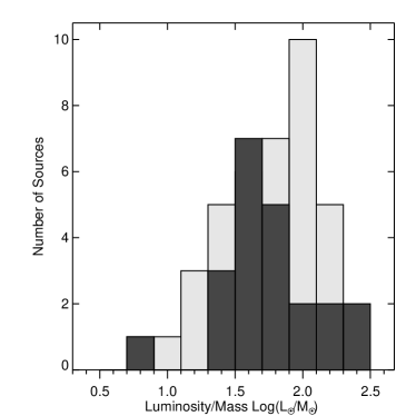
Figure 15: Histogram of the Luminosity/Mass ratio for MYSOs and Hii regions, respectively, in light and dark grey bars. Both a KS and Mann-Whitney U test cannot distinguish MYSOs and Hii regions as different distributions.

7 Summary

The core parameters of 94 sources (of 99) MYSOs and Hii regions selected as outflow candidates representative of the pre-2008 RMS survey, have been established. The sample is reduced to 89 when enforcing the distance limit of 6 kpc and is still representative of massive protostars across the MYSO to Hii region transition in the up-to-date RMS survey that now meet the original selection criteria.

The majority of the cores exhibit a single, Gaussian C¹⁸O line profile. Larson-like relationships (FWHM linewidth relationships with luminosity, radius and mass) are found for all the cores, though the scaling for these is not continuous with other studies of larger-scale molecular clouds. The most fundamental relationship is between mass and core radius, which gives rise to a surface density independent of radius. We note, however, that the scatter in the surface density in this relation is well explained by the correlation with gas opacity and agrees with models in which Larson-style relations arise due to the observed surface or column density limits. We find two possible fundamental planes in this work, representing core evolution (mass-luminosity-radius) and likely virial contributions (mass-radius-FWHM). All cores appear to be virialised $M_{\rm core}$ $\sim$ $M_{\rm vir}$. Core parameters on the observed scales are interpreted as being set prior to the onset of star formation and are not subsequently effected by the feedback from the massive protostars.

A correlation is found between the dust-continuum masses and the core (gas) masses established from the C¹⁸O emission. At the resolution of the observations, both the dust-continuum emission and C¹⁸O emission trace the same material and structures in both MYSO and Hii regions. The small differences found are all consistent with dust being a better tracer of diffuse low density gas on larger scales, whereas the C¹⁸O traces the dense hearts of the molecular clumps.

The sources are consistent with most of the luminosity arising in a single massive protostar (or central ZAMS stars for the Hii regions). The tight banding of all sources in the M-L plot, accounting for scatter, indicates a similar evolutionary stage for both the MYSOs and Hii regions investigated. This means they are ideal candidates to investigate relationships between outflow and source properties between the source types to be detailed in an upcoming paper.

Further development of the RMS survey database is required with higher spatial resolution at millimetre/sub-millimetre wavelengths to understand how the core masses are specifically related to the immediate regions surrounding the most massive protostars on arcsecond scales. This will allow us to investigate whether the mass distributions are different for MYSOs and Hii regions, if CO depletion is present in these cores and on what spatial scale, whether cores have further velocity sub-structure influenced by outflows, and how Larson-type relationships hold below 0.1 pc scales.

Appendix A Temperature, optical depth, column density and mass calculations

In this appendix the column density and mass equations are derived following from the result of Garden et al. (1991), except for the CO(3$-$2) transition. The total column density of a linear, rigid rotor molecule under conditions of local thermodynamic equilibrium (LTE), with the populations of all levels characterised by a single excitation temperature, $T_{\rm ex}$, is obtained from the integral of the optical depth over the line profile:

$$N_{\rm tot}=\frac{3k}{8\pi^{3}B\mu^{2}}\,\frac{{\rm exp}[hBJ(J+1)/kT_{\rm ex}]}{(J+1)}\,\frac{T_{\rm ex}+hB/3k}{[1-{\rm exp}(-h\nu/kT_{\rm ex})]}\int\tau_{\rm\upsilon}\,d\upsilon\;$$ (5)

where $B$ is the rotational constant, $\mu$ is the permanent dipole moment of the molecule and $J$ is the rotational quantum number of the lower state, in this case $J=2$ for the CO(3$-$2) transition. $k$ and $h$ are the Boltzmann and Planck constants respectively.

Both the excitation temperature $T_{ex}$ and optical depth $\tau_{18}$ are solved for. Assuming both the source function and initial intensity are blackbodies at the respective temperatures $T_{\rm ex}$ and $T_{\rm cmb}$ = 2.73 K, then

$$T_{\rm mb}=\frac{h\nu}{k}\left[\frac{1}{{\rm exp}(h\nu/kT_{\rm ex})-1}-\frac{1}{{\rm exp}(h\nu/kT_{\rm cmb})-1}\right]\times\,\left[1-{\rm exp}(-\tau)\right]\;,$$ (6)

for any line transition. From Equation 6 the excitation temperature, $T_{\rm ex}$, can be derived, provided the optical depth of the line is known. The ¹³CO observed simultaneously with C¹⁸O should be optically thick at the locations of peak emission in our cores, such that as $\tau_{13}\rightarrow\infty$, $[1-{\rm exp}(-\tau)]\rightarrow$ 1. In the case that C¹⁸O is optically thin, we first calculate the optical depth of $\tau_{13}$ directly from the ratio of the observed ¹³CO and C¹⁸O antenna temperatures, in order to confirm ¹³CO is thick:

$$\frac{T_{\rm mb,13}}{T_{\rm mb,18}}\simeq\frac{1-e^{-\tau_{13}}}{1-e^{-\tau_{18}}}=\frac{1-e^{-\tau_{13}}}{1-e^{(-\tau_{13}/{\rm R})}}$$ (7)

where $R$ is abundance ratio of [¹³CO]/[C¹⁸O] derived from,

$$\frac{[^{16}{\rm O}]/[^{18}{\rm O}]}{[^{12}{\rm C}]/[^{13}{\rm C}]}=\frac{58.8\times{D_{\rm gc}}+37.1}{7.5\times{D_{\rm gc}}+7.6}$$ (8)

following Wilson & Rood (1994) and $D_{\rm gc}$ is Galactocentric distance in kpc.

The excitation temperature of ¹³CO is now calculated. Rearranging Equation 6 and substituting in the numerically established optical depth, $\tau_{13}$,

$$T_{\rm ex}=\frac{15.86}{{\rm ln}\left[1+15.86/\left(\{T_{\rm mb,13}/(1-{\rm exp}(-\tau_{13}))\}+0.047\right)\right]},$$ (9)

where ${h\nu}(^{13}{\rm CO})/{k}$ = 15.86 K, with $\nu(^{13}{\rm CO})$ = 330.58 GHz and $T_{\rm mb,13}$ is the main-beam brightness temperature of the ¹³CO emission.

The C¹⁸O excitation temperature $T_{\rm ex}$ is assumed to be the same as that of the ¹³CO line, and thus the optical depth, $\tau_{18}$ can now be calculated for the C¹⁸O emission from:

$$\tau_{18}=-{\rm ln}\,\bigg{[}1-\frac{T_{\rm mb,18}}{15.80/[{\rm exp}(15.80/T_{\rm ex})-1]-0.045}\bigg{]}$$ (10)

Here the approximation for $\int\tau_{\rm\upsilon}\,d\upsilon\$ follows Buckle et al. (2010) for the case where $\tau\,\neq\,$0:

$$\int\tau_{\rm\upsilon}\,d\upsilon\,=\left[\frac{h\nu}{k}\left(\frac{1}{{\rm exp}(h\nu/kT_{\rm ex})-1}-\frac{1}{{\rm exp}(h\nu/kT_{\rm cmb})-1}\right)\right]^{-1}\,\frac{\tau}{[1-{\rm exp}(-\tau)]}\,\int T_{\rm mb}\,d\upsilon\,$$ (11)

The brightness temperature, $T_{\rm mb}$, is the antenna temperature of the telescope divided by the beam efficiency, T${}^{*}_{\rm A}$/$\eta_{\rm mb}$, and corresponds to the Rayleigh-Jeans brightness of a source minus the brightness of the cosmic microwave background with temperature, $T_{\rm cmb}$ = 2.73 K, over the beam. Combining equations 5 and 11, in the limit where $T_{\rm ex}$ $\gg$ $T_{\rm cmb}$ results in the column density:

$$N=\frac{3k}{8\pi^{3}B\mu^{2}}\,\frac{{\rm exp}[hBJ(J+1)/kT_{\rm ex}]}{(J+1)}\,\frac{1}{(h\nu/k)}\,\frac{T_{\rm ex}+hB/3k}{[{\rm exp}(-h\nu/kT_{\rm ex})]}\,\int T_{\rm mb}\,\frac{1}{[1-{\rm exp}(-\tau)]}\,d\upsilon\$$ (12)

where the permanent dipole moment for C¹⁸O is 0.1101 Debye (Chackerian & Tipping, 1983). Conforming to cgs units typically used in such analysis $B$=58.14 GHz, $k$=1.381$\times$10^-16 erg K^-1, h=6.626$\times$10^-27 erg s, $\nu$(C¹⁸O) = 329.33055 GHz, velocity $\upsilon$ is in k ms^-1, $\mu$(C¹⁸O) = 0.1101 $\times$10^-18 StatC cm (where 1 statC = 1 g^1/2 cm^3/2 s⁻¹ = 1 erg^1/2 cm^1/2), $\tau$ becomes $\tau_{18}$, the calculated optical depth of the C¹⁸O line calcualted in Equation 10 and $T_{\rm ex}$ is the calculated excitation temperature from Equation 9. The column density for the C¹⁸O (3$-$2) transition is therefore:

$$N({\rm C^{18}O})=5.0\,{\times}\,10^{12}\,\frac{{\rm exp}(16.74/T_{\rm ex})\,(T_{\rm ex}+0.93)}{{\rm exp}(-15.80/T_{\rm ex})}\,\int T_{\rm mb}\,\frac{\tau_{18}}{[1-{\rm exp}(-\tau_{18})]}\,d\upsilon\;,{\rm cm}^{-2}$$ (13)

The mass of a source can then be calculated from the column density via:

$$M_{\rm gas}=N({\rm CO})\bigg{[}\frac{{\rm H_{2}}}{\rm C^{18}O}\bigg{]}\mu_{g}\,m(_{\rm H_{2}})\Omega\,D^{2}$$ (14)

where $\mu_{g}$ = 1.36 is the total gas mass relative to H₂, the abundance ratio $[\rm H_{2}/C^{18}O]$ is a combination of ${\rm H_{2}}/{\rm{}^{12}CO}$ = 10⁴ and ${\rm{}^{16}O}/{\rm{}^{18}O}$ = 58.8 $\times$ $D_{\rm GC}$(kpc) $+$ 37.1 (Wilson & Rood, 1994), where $D_{\rm GC}$ is the Galactocentric distance and $D$ is the distance of the source to the Sun, both in kpc. $\Omega$ is the solid angle corresponding to the emission in one pixel of the maps used in this work. Thus including the conversion factors the core gas mass in solar masses (M_⊙) is calculated for every pixel of the map using Equation 15. The total core mass is the summation within the defined aperture encompassing the core, as described in Section 3.

$$M_{\rm gas}\,({\rm M}_{\odot})=2.5\,{\times}\,10^{-12}\,\theta^{2}(\arcsec)\,D^{2}({\rm kpc})\,\bigg{[}\frac{\rm H_{2}}{\rm C^{18}O}\bigg{]}\,\frac{{\rm exp}(16.74/T_{\rm ex})\,(T_{\rm ex}+0.93)}{{\rm exp}(-15.80/T_{\rm ex})}\,\int T_{\rm mb}\,\frac{\tau_{18}}{[1-{\rm exp}(-\tau_{18})]}\,d\upsilon$$ (15)

Figure 16: Correction factor between calculated LTE calculated column density and that input into radex. Although at 20 K the correction factor is $\sim$2 at 10⁴ cm^-3, at the average volume density of the cores ($\sim$7$\times$10⁴ cm^-3) the correction factor is $\sim$ unity even at 20 K.

The LTE approximation is only valid if the volume density is sufficient enough (n$\gtrsim$n_crit = $\sim$3.2$\times$10⁴ cm^-3) such that the excitation temperature can be assumed to be equal to the kinetic temperature. If this is not the case (T${}_{\rm ex}\,<$ T_kin) the LTE calculation will underestimate the column density and therefore mass. These parameters are then subject to a correction factor dependent on excitation temperature and volume density. Figure 16 shows the correction factor as a function of volume density for kinetic temperatures of 20, 30 and 40 K (i.e. the input excitation temperatures in LTE calculations). The factor is calculated by comparison of the input column density into radex (van der Tak et al., 2007) and that calculated via LTE calculation here. A representative H₂ column density of 2$\times$10²² cm^-2 and a linewidth of the average of all cores are used as inputs. At 20 K for a 10⁴ cm^-3 volume density (just below critical), the correction factor required to obtain the correct column density from the presented LTE assumption is $\sim$2. Above the critical density the correction factor approaches unity. The average volume density of the cores however is $\sim$7$\times$10⁴ cm^-3 calculated using the LTE masses and deconvolved radii. Thus the LTE assumption is valid as the correction factor at this volume density is $\sim$ unity. There is no evidence for sub-thermal excitation of the CO $J$=3$-$2 transition.

References

- Ao et al. (2004) Ao Y., Yang J., Sunada K., 2004, AJ, 128, 1716
- Ballesteros-Paredes et al. (2011) Ballesteros-Paredes J., Hartmann L. W., Vázquez-Semadeni E., Heitsch F., Zamora-Avilés M. A., 2011, MNRAS, 411, 65
- Beltrán et al. (2013) Beltrán M. T. et al., 2013, A&A, 552, A123
- Bergin et al. (1995) Bergin E. A., Langer W. D., Goldsmith P. F., 1995, ApJ, 441, 222
- Beuther et al. (2002) Beuther H., Schilke P., Menten K. M., Motte F., Sridharan T. K., Wyrowski F., 2002, ApJ, 566, 945
- Bontemps et al. (2010) Bontemps S., Motte F., Csengeri T., Schneider N., 2010, A&A, 524, A18
- Buckle et al. (2010) Buckle J. V. et al., 2010, MNRAS, 401, 204
- Buckle et al. (2009) Buckle J. V. et al., 2009, MNRAS, 399, 1026
- Burkert & Hartmann (2013) Burkert A., Hartmann L., 2013, ApJ, 773, 48
- Caselli et al. (1999) Caselli P., Walmsley C. M., Tafalla M., Dore L., Myers P. C., 1999, ApJL, 523, L165
- Cesaroni et al. (2007) Cesaroni R., Galli D., Lodato G., Walmsley C. M., Zhang Q., 2007, Protostars and Planets V, 197
- Chackerian & Tipping (1983) Chackerian, Jr. C., Tipping R. H., 1983, Journal of Molecular Spectroscopy, 99, 431
- Curtis & Richer (2011) Curtis E. I., Richer J. S., 2011, MNRAS, 410, 75
- Davies et al. (2011) Davies B., Hoare M. G., Lumsden S. L., Hosokawa T., Oudmaijer R. D., Urquhart J. S., Mottram J. C., Stead J., 2011, MNRAS, 416, 972
- Davies et al. (2010) Davies B., Lumsden S. L., Hoare M. G., Oudmaijer R. D., de Wit W.-J., 2010, MNRAS, 402, 1504
- Di Francesco et al. (2008) Di Francesco J., Johnstone D., Kirk H., MacKenzie T., Ledwosinska E., 2008, ApJS, 175, 277
- Du & Yang (2008) Du F., Yang J., 2008, ApJ, 686, 384
- Elia et al. (2010) Elia D. et al., 2010, A&A, 518, L97
- Elmegreen & Falgarone (1996) Elmegreen B. G., Falgarone E., 1996, ApJ, 471, 816
- Evans et al. (2014) Evans, II N. J., Heiderman A., Vutisalchavakul N., 2014, ApJ, 782, 114
- Faúndez et al. (2004) Faúndez S., Bronfman L., Garay G., Chini R., Nyman L.-Å., May J., 2004, A&A, 426, 97
- Fontani et al. (2006) Fontani F., Caselli P., Crapsi A., Cesaroni R., Molinari S., Testi L., Brand J., 2006, A&A, 460, 709
- Fontani et al. (2012) Fontani F., Giannetti A., Beltrán M. T., Dodson R., Rioja M., Brand J., Caselli P., Cesaroni R., 2012, MNRAS, 423, 2342
- Fuller et al. (2005) Fuller G. A., Williams S. J., Sridharan T. K., 2005, A&A, 442, 949
- Garden et al. (1991) Garden R. P., Hayashi M., Hasegawa T., Gatley I., Kaifu N., 1991, ApJ, 374, 540
- Gibson et al. (2009) Gibson D., Plume R., Bergin E., Ragan S., Evans N., 2009, ApJ, 705, 123
- Ginsburg et al. (2013) Ginsburg A. et al., 2013, ApJS, 208, 14
- Goodman et al. (1998) Goodman A. A., Barranco J. A., Wilner D. J., Heyer M. H., 1998, ApJ, 504, 223
- Harris et al. (2010) Harris A. I., Baker A. J., Zonak S. G., Sharon C. E., Genzel R., Rauch K., Watts G., Creager R., 2010, ApJ, 723, 1139
- Heiderman et al. (2010) Heiderman A., Evans, II N. J., Allen L. E., Huard T., Heyer M., 2010, ApJ, 723, 1019
- Heyer et al. (2009) Heyer M., Krawczyk C., Duval J., Jackson J. M., 2009, ApJ, 699, 1092
- Hill et al. (2005) Hill T., Burton M. G., Minier V., Thompson M. A., Walsh A. J., Hunt-Cunningham M., Garay G., 2005, MNRAS, 363, 405
- Hoare & Franco (2007) Hoare M. G., Franco J., 2007, Massive Star Formation, Hartquist, T. W., Pittard, J. M., & Falle, S. A. E. G., ed., Springer Dordrecht, p. 61
- Hosokawa & Omukai (2009) Hosokawa T., Omukai K., 2009, ApJ, 691, 823
- Hosokawa et al. (2010) Hosokawa T., Yorke H. W., Omukai K., 2010, ApJ, 721, 478
- Isobe et al. (1990) Isobe T., Feigelson E. D., Akritas M. G., Babu G. J., 1990, ApJ, 364, 104
- Jackson et al. (2006) Jackson J. M. et al., 2006, ApJS, 163, 145
- Kauffmann & Pillai (2010) Kauffmann J., Pillai T., 2010, ApJL, 723, L7
- Kauffmann et al. (2013) Kauffmann J., Pillai T., Goldsmith P. F., 2013, ApJ, 779, 185
- Kauffmann et al. (2010) Kauffmann J., Pillai T., Shetty R., Myers P. C., Goodman A. A., 2010, ApJ, 712, 1137
- Kennicutt (1998) Kennicutt, Jr. R. C., 1998, ARA&A, 36, 189
- Kirk et al. (2013) Kirk J. M. et al., 2013, MNRAS, 432, 1424
- Klaassen & Wilson (2007) Klaassen P. D., Wilson C. D., 2007, ApJ, 663, 1092
- Krumholz et al. (2012) Krumholz M. R., Dekel A., McKee C. F., 2012, ApJ, 745, 69
- Krumholz & Thompson (2007) Krumholz M. R., Thompson T. A., 2007, ApJ, 669, 289
- Kutner & Ulich (1981) Kutner M. L., Ulich B. L., 1981, ApJ, 250, 341
- Lada & Lada (2003) Lada C. J., Lada E. A., 2003, ARA&A, 41, 57
- Lada et al. (2010) Lada C. J., Lombardi M., Alves J. F., 2010, ApJ, 724, 687
- Larson (1981) Larson R. B., 1981, MNRAS, 194, 809
- Lombardi et al. (2010) Lombardi M., Alves J., Lada C. J., 2010, A&A, 519, L7
- Longmore et al. (2007) Longmore S. N., Burton M. G., Barnes P. J., Wong T., Purcell C. R., Ott J., 2007, MNRAS, 379, 535
- López-Sepulcre et al. (2010) López-Sepulcre A., Cesaroni R., Walmsley C. M., 2010, A&A, 517, A66
- Lumsden et al. (2013) Lumsden S. L., Hoare M. G., Urquhart J. S., Oudmaijer R. D., Davies B., Mottram J. C., Cooper H. D. B., Moore T. J. T., 2013, ApJS, 208, 11
- Lumsden et al. (2003) Lumsden S. L., Puxley P. J., Hoare M. G., Moore T. J. T., Ridge N. A., 2003, MNRAS, 340, 799
- MacLaren et al. (1988) MacLaren I., Richardson K. M., Wolfendale A. W., 1988, ApJ, 333, 821
- Mardones et al. (1997) Mardones D., Myers P. C., Tafalla M., Wilner D. J., Bachiller R., Garay G., 1997, ApJ, 489, 719
- McKee & Tan (2003) McKee C. F., Tan J. C., 2003, ApJ, 585, 850
- Molinari et al. (2008) Molinari S., Pezzuto S., Cesaroni R., Brand J., Faustini F., Testi L., 2008, A&A, 481, 345
- Mottram et al. (2011a) Mottram J. C. et al., 2011a, ApJL, 730, L33
- Mottram et al. (2011b) Mottram J. C. et al., 2011b, A&A, 525, A149
- Ossenkopf & Henning (1994) Ossenkopf V., Henning T., 1994, A&A, 291, 943
- Salaris & Cassisi (2006) Salaris M., Cassisi S., 2006, Evolution of Stars and Stellar Populations
- Shepherd et al. (2000) Shepherd D. S., Yu K. C., Bally J., Testi L., 2000, ApJ, 535, 833
- Shu et al. (1987) Shu F. H., Adams F. C., Lizano S., 1987, ARA&A, 25, 23
- Urquhart et al. (2008) Urquhart J. S. et al., 2008, A&A, 487, 253
- Urquhart et al. (2014a) Urquhart J. S., Figura C. C., Moore T. J. T., Hoare M. G., Lumsden S. L., Mottram J. C., Thompson M. A., Oudmaijer R. D., 2014a, MNRAS, 437, 1791
- Urquhart et al. (2012) Urquhart J. S. et al., 2012, MNRAS, 420, 1656
- Urquhart et al. (2014b) Urquhart J. S. et al., 2014b, MNRAS, 443, 1555
- Urquhart et al. (2011) Urquhart J. S. et al., 2011, MNRAS, 418, 1689
- Urquhart et al. (2013) Urquhart J. S. et al., 2013, MNRAS, 435, 400
- van der Tak et al. (2007) van der Tak F. F. S., Black J. H., Schöier F. L., Jansen D. J., van Dishoeck E. F., 2007, A&A, 468, 627
- Wall & Jenkins (2003) Wall J. V., Jenkins C. R., 2003, Practical Statistics for Astronomers, Ellis R., Huchra J., Kahn S., Rieke G., Stetson P. B., eds. Cambridge University Press
- Wienen et al. (2012) Wienen M., Wyrowski F., Schuller F., Menten K. M., Walmsley C. M., Bronfman L., Motte F., 2012, A&A, 544, A146
- Wilson & Rood (1994) Wilson T. L., Rood R., 1994, ARA&A, 32, 191
- Yıldız et al. (2012) Yıldız U. A., Kristensen L. E., van Dishoeck E. F., Belloche A., van Kempen T. A., Hogerheijde M. R., Güsten R., van der Marel N., 2012, A&A, 542, A86
- Zhang & Gao (2009) Zhang L.-Y., Gao Y., 2009, CA&A, 33, 32
- Zhang et al. (2014) Zhang Y., Tan J. C., Hosokawa T., 2014, ApJ, 788, 166