A Telescopic Binary Learning Machine for Training Neural Networks

Abstract

This paper proposes a new algorithm based on multi-scale stochastic local search with binary representation for training neural networks.

In particular, we study the effects of neighborhood evaluation strategies, the effect of the number of bits per weight and that of the maximum weight range used for mapping binary strings to real values. Following this preliminary investigation, we propose a telescopic multi-scale version of local search where the number of bits is increased in an adaptive manner, leading to a faster search and to local minima of better quality. An analysis related to adapting the number of bits in a dynamic way is also presented. The control on the number of bits, which happens in a natural manner in the proposed method, is effective to increase the generalization performance.

Benchmark tasks include a highly non-linear artificial problem, a control problem requiring either feed-forward or recurrent architectures for feedback control, and challenging real-world tasks in different application domains. The results demonstrate the effectiveness of the proposed method.

I Introduction

Machine learning and optimization share a long common history: machine learning implies optimizing the performance of the trained system measured on the examples, with possible early stopping or additional regularizing terms in the function to avoid overtraining and increase generalization.

Starting from back-propagation [1, 2], most techniques for training neural networks use continuous optimization schemes based on partial derivatives, like gradient descent and variations thereof, while Support Vector Machines (SVMs) use quadratic optimization [3]. Recent proposals to simplify the optimization task by creating a randomized first layer and limiting optimization to the last-layer weights are extreme learning [4] and reservoir computing [5].

Different methods consider Combinatorial Optimization (CO) techniques without derivatives, like Simulated Annealing and Genetic Algorithms, see [6] for a comparative analysis. In most CO techniques, weights are considered as binary strings and the operators acting during optimization change bits, either individually (like with mutation in GA) or more globally (like with cross-over operators in GA). Methods for the optimization of functions of real variables with no derivatives are an additional option, for example direct search [7] or versions of Simulated Annealing for functions of continuous variables [8]. Intelligent schemes based on adaptive diversification strategies by prohibiting selected moves in the neighborhood are considered in [9].

A strong motivation for considering techniques with no derivatives is when derivatives are not always available, for example in threshold networks [10], because their transfer functions are discontinuous. Preliminary results for threshold networks are presented in [11].

This paper aims at considering neural networks with smooth input-output transfer functions and proposes a new method, called Telescopic Binary Learning Machine (BLM for short), that combines stochastic local search optimization with the discrete representation of network parameters (weights). The technique is suitable both for feed-forward and recurrent networks, and can also be applied to the control of dynamic systems with feedback.

The paper is organized as follows: in Sec. II we introduce the SLS techniques that will be used for the optimization of network parameters; in Sec. III we describe the specific building blocks and algorithmic choices that enable the BLM algorithm; in Sec. IV we use a highly non-linear benchmark task to develop insight and drive the choice of specific algorithms and parameters; in Sec. V we apply the network to a well-known control problem and test the suitability of BLM for training recurrent networks; in Sec. VI we test the technique on a set of classic real-world benchmark problems and compare it with state-of-the-art derivative-based and derivative-free methods. Finally, in Sec. VII we draw some conclusions and indicate possible further developments.

II Local search on highly structured fitness surfaces

Local search is a basic building block of most heuristic search methods for combinatorial optimization. It consists of starting from an initial tentative solution and trying to improve it through repeated small changes. At each repetition the current is perturbed and the function to be optimized is tested. The change is kept if the new solution is better, otherwise another change is tried. The function $f(X)$ to be optimized is called fitness function, goodness function, or objective function.

In a way, gradient-based techniques like back-propagation (BP) also consider the effect of small local changes. In BP the effect of the tentative change is approximated by the local linear model: the scalar product between gradient and displacement. When no analytic derivatives are available, the derivatives can be approximated by finite differences. One is therefore dealing with techniques based on gradual changes evaluated through their effect on the error function, but considering individual bits leads to a radical simplification, and to a natural multi-scale structure because of the binary representation (change of the $i$-th bit leads to a change proportional to $2^{i}$).

Let’s define the notation. $\mathcal{X}$ is the search space, $f(X)$ the function to be optimized, $X^{(t)}$ is the current solution at iteration (“time”) $t$. $N(X^{(t)})$ is the neighborhood of point $X^{(t)}$, obtained by applying a set of basic moves $\mu_{0},\dots,\mu_{M}$ to the current configuration:

$$N(X^{(t)})=\{X\in\mathcal{X}\quad:\quad X=\mu_{i}(X^{(t)}),i=0,\dots,M\}.$$

If the search space is given by binary strings with a given length $L$, then $\mathcal{X}=\{0,1\}^{L}$, the moves can be those changing (or complementing or flipping) the individual bits, and therefore $M$ is equal to the string length $L$.

Local search starts from an admissible configuration $X^{(0)}$ and builds a trajectory $X^{(0)},\dots,X^{(t+1)}$. The successor of the current point is a point in the neighborhood with a lower value of the function $f$ to be minimized:

$$Y \leftarrow \textsc{Improving-Neighbor}\bigl{(}N(X^{(t)})\bigr{)}$$

$$X^{(t+1)} = \begin{cases}Y&\text{if $f(Y)<f(X^{(t)})$}\\ X^{(t)}&\text{otherwise (search stops)}.\end{cases}$$

Function Improving-Neighbor returns an improving element in the neighborhood. In a simple case this is the element with the lowest $f$ value, but other possibilities exist, for example the first improving neighbor encountered. If no neighbor has a better $f$ value, i.e., if the configuration is a local minimizer, the search stops.

Local search is surprisingly effective because most combinatorial optimization problems have a very rich internal structure relating the configuration $X$ and the $f$ value. If one starts at a good solution, solutions of similar quality can, on the average, be found more in its neighborhood than by sampling a completely unrelated random point. A neighborhood is suitable for local search if it reflects the problem structure. Stochastic elements can be immediately added to local search to make it more robust [12], for example a random sampling of the neighborhood can be adopted instead of a trivial exhaustive consideration.

In many relevant problems local minima tend to be clustered, furthermore good local minima tend to be closer to other good minima. Let us define as attraction basin associated with a local optimum the set of points $X$ which are mapped to the given local optimum by the local search trajectory. One may think about a smooth $f$ surface in a continuous environment, with basins of attraction which tend to have a nested, “fractal” structure, like in Fig. 1. This multi-scale structure, where smaller valleys are nested within larger ones, is the basic motivation for more complex methods like Variable Neighborhood Search, Iterated Local Search (ILS), see for example [13]. This structural property is also called Big Valley property (or massif central).

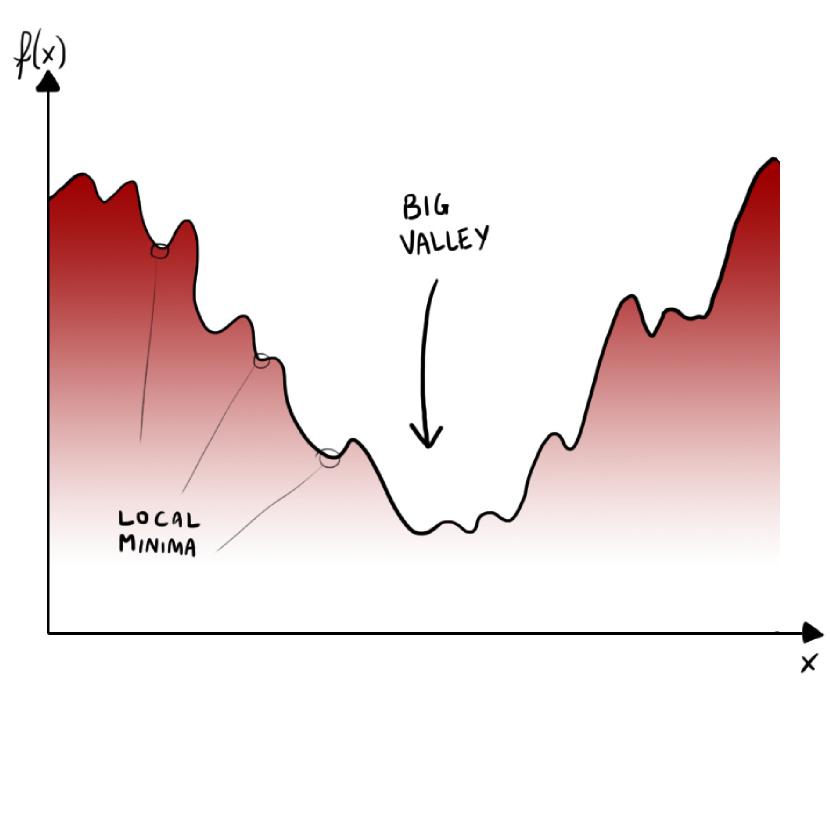
Figure 1: The massif central hypothesis: local minima tend to occur in clusters (from [14]).

In Simulated Annealing, a tentative move is generated and accepted with a probability depending on the difference in value $\Delta f$ caused by the move:

$$\Pr(\text{acceptance})\approx e^{-\frac{\Delta f}{T}}.$$

Studies and experiments of Simulated Annealing [15, 16] motivate cooling schedules (gradual reduction of the $T$ parameter controlling move acceptance) so that large temperature at the beginning causes a sampling of states regulated by the overall large-scale structure of the problem, while lower temperature at the end makes the search more sensitive to fine-scale details. The role of high temperatures is to “iron out” the fine details of the fitness surface at the beginning, to avoid the search being trapped in a poor local minimum.

Multi-scale methods which jointly solve related versions of the same problems at different scales and have been proposed in different areas, e.g. image analysis [17], modeling and computation [18], neural networks for optimization [19]. The application in [19] is for multi-scale optimization (inexact graph matching). A cubic neural network energy function is considered, a smaller coarser version of the problem is derived, and one alternates between relaxation steps for the fine-scale and coarse-scale problems.

In this paper, we consider two simple options: no diversification (where the search stops upon reaching a local optimum), and repeated local search, where the search restarts from a random configuration whenever a local optimum is attained.

In the following, the term run will refer to a sequence of moves that ends to a local minimum of the search space, while a search can refer to a sequence of runs and restarts.

In the following we illustrate the main building blocks leading to a much faster and more effective multi-scale implementation of local search for neural networks.

III The Binary Learning Machine (BLM) Algorithm

A brute-force implementation of local search consists of evaluating all possible changes of the individual bits representing the weights. For each bit change all training examples are evaluated to calculate the difference in the training error. This implementation is out of question for networks with more than a few neurons and weights, leading to enormous CPU times. This can explain why basic local search has not been considered as a competitive approach for training up to now.

In the following sections we design an algorithm, called Telescopic Binary Learning Machine (BLM for short), which uses a smart realization of local stochastic search (SLS), coupled with an efficient network representation. The term Binary Learning Machine underlines the fact that it is based on the binary representation of weights and changes acting on the individual bits.

Telescopic BLM is based on:

• Gray coding to map from binary strings to weights

• Incremental neighborhood evaluation (also called delta evaluation)

• Smart sampling of the neighborhood (stochastic “first improving” and “best improving”)

• Multi-scale (telescopic) search, gradually increasing the number of bits in a dynamic and adaptive manner

In this Section we illustrate the many choices to obtain a representation of the neural network that can be efficiently optimized by a SLS algorithm.

III-A Weight representation

The appropriate choice of representation is critical to ensure that changes of individual bits lead to an effective sampling of the neighborhood.

III-A1 Number of bits and discretization

We represent weights and biases as integral multiples of a discretization value $\epsilon>0$, with an $n$-bit two’s-complement integer as multiplier. Options $n=2,4,8,12,16,24$ have been investigated. In all tests a maximum representable weight value $w_{\text{max}}$ is given (this limitation in weight size acts as an intrinsic regularization mechanism to prevent overtraining), and $\epsilon$ is set so that the range of representable weights includes the interval $[-w_{\text{max}},w_{\text{max}}]$. As the two’s-complement representation is asymmetric, with $n$ bits actually representing the set $\{-2^{n-1},\dots,2^{n-1}-1\}$, we set

$$\epsilon=\frac{w_{\text{max}}}{2^{n-1}-1}$$ (1)

so that the maximum value $w_{\text{max}}$ can be represented; the minimum representable weight will actually be $-w_{\text{max}}-\epsilon$. Since we start from $n=2$ bits, one can always represent at least one positive and two negative weight values.

Figure 2: Neighbors of the current point with Gray coding vs. standard base-2 coding.

III-A2 Gray coding

In order to improve the correspondence between the bit-flip local moves of the BLM algorithm and the natural topology of the network’s weight space, we use Gray encoding of the $n$-bit integer multiplier. Gray encoding has the property that, starting from code $n$, the nearby codes for $n-1$ and $n+1$ are obtained by changing a single bit (i.e., they have a Hamming distance of one with respect to the code of $n$). This choice allows the generic value $h\epsilon$, $h$ being an $n$-bit integer, to reach its neighboring values $(h+1)\epsilon$ and $(h-1)\epsilon$ by a single move, while in the conventional binary coding one of the two neighbors could be removed by as much as $n$ moves, namely when moving from $0$ to $-1$ (represented as $00\cdots 0$ and $11\cdots 1$ in two’s complement standard binary).
Given a weight $w$, by changing one of the $n$ bits in the encoding (and by repeating the operation for all possible bits), one obtains $n$ weights in the neighborhood. As shown in Fig. 2, for the cited property of the Gray code, the neighborhood always contains the nearest weights on the discretized grid, plus a cloud of points at growing distances in weight space.

III-B Memory-based incremental neighborhood evaluation

Let $N_{\text{layers}}$ be the number of network layers (hidden and outputs); the input layer is layer 0, while layer $N_{\text{layers}}$ is the output. For $l=0,\dots,N_{\text{layers}}$, let $n_{l}$ be the number of neurons in layer $l$. For $j=1,\dots,n_{l}$, let $o^{l}_{j}$ be the output of neuron $j$ in layer $l$. Thus, $o^{0}_{j}$ is the value of the $j$-th input. Let $f^{l}(x)$ be the transfer function of neurons at layer $l$, and $w^{l}_{ij}$ be the weight connecting neuron $i$ at layer $l-1$ to neuron $j$ at layer $l$. Starting from the input values, the feed-forward computation consists of iterating the following operation for $l=1,\dots,N_{\text{layers}}$:

$$o^{l}_{j}=f^{l}(s^{l}_{j}),\qquad\text{where}\qquad s^{l}_{j}=b^{l}_{j}+\sum_{i=1}^{n_{l-1}}w^{l}_{ij}o^{l-1}_{i}.$$ (2)

The simple bit-flip neighborhood scheme chosen for this investigation requires a large number of steps, each consisting of the modification of a single weight. A very significant speedup can be obtained by storing the $s^{l}_{j}$ values for all neurons and all samples. In order to obtain the network output when weight $w^{L}_{IJ}$ is replaced by a new value $W$, the following algorithm provides a faster incremental evaluation:

1. Recompute the output of neuron $J$ in layer $L$:

   $$o^{\prime L}_{J}=f^{L}\bigl{(}s^{L}_{J}+(W-w^{L}_{IJ})o^{L-1}_{I}\bigr{)}.$$

   If $L=N_{\text{layers}}$, the $J$-th network output is $o^{\prime L}_{J}$, the others are unchanged. Stop.

2. Let the output variation be

   $$\Delta o^{L}_{J}=o^{\prime L}_{J}-o^{L}_{J}.$$

3. Recompute all contributions of output $o^{L}_{J}$ to the neurons of the next layer, for $k=1,\dots,n_{L+1}$:

   $$s^{\prime L+1}_{k}=s^{L+1}_{k}+w^{L+1}_{Jk}\Delta o^{L}_{J};$$

   $$o^{\prime L+1}_{k}=f^{L+1}(s^{\prime L+1}_{k}).$$

4. If there are other layers, apply (2) for $l=L+2,\dots,N_{\text{layers}}$.

Obvious modifications apply for bias values.

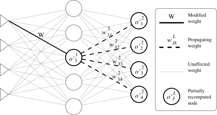
Figure 3: Affected neurons in an incremental evaluation step with a single changed weight in the input layer.

Consider the case shown in Fig. 3, where $N_{\text{layers}}=2$ (single hidden layer). Upon modification of an input weight, the update procedure requires $O(1)$ operations per sample to update the output of the only affected hidden neuron, and $O(n_{2})$ operations to recompute the contributions of that hidden neuron on all outputs. Upon modification of an output weight, the whole incremental procedure requires $O(1)$ calculations for recomputing the affected output neuron. On average, since the network contains $O(n_{0}n_{1})$ input weights and $O(n_{1}n_{2})$ output weights, an incremental computation requires $O\bigl{(}n_{0}n_{2}/(n_{0}+n_{2})\bigr{)}$ operations.

For comparison, the number of operations required by the complete feed-forward procedure is roughly proportional to the number of weights in the network, i.e., $O\bigl{(}n_{1}(n_{0}+n_{2})\bigr{)}$. An incremental search step on the largest benchmark considered is faster by about two orders of magnitude with respect to the complete evaluation.

III-C Neighborhood exploration

An important parameter for the implementation of a local search heuristic is the fraction of neighborhood that the algorithm explores before moving, and two extreme cases are:

• Best move — all feasible moves are checked, and the one leading to the best improvement in the target function is selected. Ties may be broken randomly or by considering secondary objectives.

• First improving move — feasible moves are explored in random order, and the first move that leads to an improvement of the target objective is selected.

Preliminary tests of the BLM algorithm suggest that the Best move strategy causes a serious slowdown of each iteration and, while having a steeper initial improvement, it can lead to more over-training. Therefore, in the remainder of our work we shall only consider the First-move strategy.

Since the search starts from a random configuration, at the beginning most moves are improving, and the algorithm only needs to scan a small subset before finding one. As the search proceeds, the average number of neighbors that must be evaluated increases. The fraction, however, does not become very large until the local minimum is close, and remains in the $10\%$ range for most of the run.

The combination of incremental evaluation and first-improving strategy lead to an approximate speedup in the order of 100 times with respect to the baseline algorithm for the benchmark problems considered.

III-D Multi-scale network representation (Telescopic BLM)

Given the potentially large number of weights in a fully connected feed-forward neural network, its discrete $n$-bit representation can be large, leading to slow improvements. The Telescopic variant of BLM starts with a coarser representation where only the most significant $n^{\prime}$ bits per weight (e.g., $n^{\prime}=2$) are allowed to change. This allows for a quick, large-scale exploration of the search space. Periodically, the number $n^{\prime}$ of flippable bits is increased, until the full-fledged $n$-bit search takes place.

As the search proceeds, therefore, the neighborhood structure of the problem becomes richer and richer; moreover, the most significant bits are always allowed to flip, therefore the search algorithm is never restrained in small regions as the search proceeds (as is often the case with backpropagation and learning-rate-decay mechanisms).

The decision to increase the number $n^{\prime}$ of unlocked bits can be linked in an adaptive manner to the current search results. The simplest criterion is to increase $n^{\prime}$ whenever a local minimum of the loss function is reached for the current neighborhood structure. In this case, an additional bit is “unfrozen” and available for tests and possible changes.

III-E Telescopic threshold adjustment

Instead of waiting until a local minimum is found, one can increase the number of bits in the weight representation of the BLM algorithm whenever the number of improving neighbors falls below a certain threshold (e.g., expressed as a fraction of the total number of possible moves in the neighborhood).

In a first-improvement scenario, we cannot directly determine the desired number. Therefore, we need to efficiently estimate it.

Below, we proceed by first analyzing the inverse problem (a), then we use the solution to determine a threshold (b).

III-E1 Computing the expected number of moves before improvement

Let $A_{N}$ be the set of $N=2^{n_{\text{weights}}n^{\prime}}$ local moves, $k$ of which are improving. We want to compute the expected number of moves to be tested before we find one of the $k$ improving ones. Moves are randomly selected, therefore we can assume that the $k$ improving moves are randomly distributed in $A_{N}$. Therefore, our problem is equivalent to the following:
Let

$$A_{N}=\{0,\dots,N-1\}$$

be the set of the first $N$ natural numbers. Given the natural number $1\leq k\leq N$, we want to determine the expected value of the minimum element in subsets of $A_{N}$ of cardinality $k$:

$$E_{k,N}=E(\min X:X\subseteq A_{N}\wedge|X|=k).$$

Let us define $s_{m,k,N}$ as the number of subsets of $A_{N}$ having cardinality $k$ and minimum $m$:

$$s_{m,k,N}=|\{X\subseteq A_{N}:|X|=k\wedge\min X=m\}|.$$

The following inductive relationship holds:

$$s_{m,k,N}=\begin{cases}\displaystyle\binom{N-1}{k-1}&\text{if $m=0$}\\ s_{m-1,k,N-1}&\text{if $1\leq m\leq N-k$}\\ 0&\text{otherwise.}\end{cases}$$

In fact, if $m=0$ then $0\in X$, and to complete such a set $X$ we have to select its remaining $k-1$ elements among the remaining $N-1$ nonzero elements of $A_{N}$. Moreover, the minimum of any set $X\subseteq A_{N}$ containing $k$ elements is at most $N-k$, therefore if $m>N-k$ then $s_{m,k,N}=0$. In all other cases, the number of such subsets is equivalent to the number of subsets of cardinality $k$ of $A_{N-1}$ having minimum $m-1$ (remove $0$ from $A_{N}$ and subtract $1$ from all elements).
Therefore, let $p_{m,k,N}$ be the probability that a subset of cardinality $k$ of $A_{N}$ has minimum $m$:

$$p_{m,k,N} = \Pr(\min X=m:X\subseteq A_{N}\wedge|X|=k)$$

$$= {\binom{N}{k}}^{-1}s_{m,k,N};$$

then,

$$E_{k,N}=\sum_{m=0}^{N-k}m\cdot p_{m,k,N}={\binom{N}{k}}^{-1}\sum_{m=1}^{N-k}ms_{m,k,N}$$

$$={\binom{N}{k}}^{-1}\left(\sum_{m=1}^{N-k}s_{m,k,N}+\sum_{m=1}^{N-k}(m-1)s_{m-1,k,N-1}\right)$$

$$=\overbrace{{\binom{N}{k}}^{-1}\sum_{m=1}^{N-k}s_{m,k,N}}^{\alpha_{k,N}}+\overbrace{{\binom{N}{k}}^{-1}\binom{N-1}{k}E_{k,N-1}.}^{\beta_{k,N}}$$ (3)

Let us obtain a recurrence relation for the first term in (3). Clearly, $\alpha_{k,k}=0$. Otherwise, if $N>k$:

$$\alpha_{k,N} = {\binom{N}{k}}^{-1}\sum_{m=1}^{N-k}s_{m-1,k,N-1}$$

$$= {\binom{N}{k}}^{-1}\left(\binom{N-2}{k-1}+\sum_{m=1}^{N-k-1}s_{m,k,N-1}\right)$$

$$= {\binom{N}{k}}^{-1}\left(\binom{N-2}{k-1}+\binom{N-1}{k}\alpha_{k,N-1}\right)$$

$$= \frac{N-k}{N}\left(\frac{k}{N-1}+\alpha_{k,N-1}\right).$$

The term $\beta_{k,N}$ in (3) can be simplified as

$$\beta_{k,N}=\frac{N+k}{N}E_{k,N-1}.$$

By putting all pieces together, we obtain the recurrent relation for $E_{k,N}$:

$$\alpha_{k,N} = \begin{cases}0&\text{if $N=k$}\\ \displaystyle\frac{N-k}{N}\left(\frac{k}{N-1}+\alpha_{k,N-1}\right)&\text{otherwise}\end{cases}$$ (4)

$$E_{k,N} = \begin{cases}0&\text{if $N=k$}\\ \displaystyle\alpha_{k,N}+\frac{N+k}{N}E_{k,N-1}&\text{otherwise.}\end{cases}$$ (5)

III-E2 Application to telescopic BLM

Let $c_{i}$ be the number of moves that have been sequentially tested at step $i$ of the local search procedure before finding an improving one; in other words, the $c_{i}$’s play the role of index $m$ in the previous section. If we assume that the number of improving moves does not change dramatically between iterations, then a moving average of the $c_{i}$’s is an estimator of $E_{k_{i},N}$, where $k_{i}$ is the (unknown) total number of improving moves at time $i$:

$$E_{k_{i},N}\approx\mu_{i},$$ (6)

where $\mu_{0}=0$, $\mu_{i}=\eta\mu_{i-1}+(1-\eta)c_{i}$ is an exponential moving average with decay factor $\eta$.
Suppose that we want to increase the number of bits in the search space whenever the number of improving moves $k_{i}$ falls below a given threshold $\phi N$ (given as a fraction of the total number of moves $N$, with $0\leq\phi\leq 1$); since $E_{k,N}$ is a decreasing function of $k$, then the condition $k_{i}<\phi N$ is equivalent to

$$E_{k_{i},N}\geq E_{\lfloor\phi N\rfloor,N};$$

finally, by taking into account the above approximation (6), the telescopic criterion becomes

$$\mu_{i}\geq E_{\lfloor\phi N\rfloor,N}.$$

In order to use this criterion, we need to recompute the threshold $E_{\lfloor\phi N\rfloor,N}$ by using (4) and (5) whenever the number $N$ of moves changes (i.e., when the number of bits $n^{\prime}$ in the weights representation is increased), and maintain a mobile average of failed attempts per local move with a suitable decay factor $\eta$.
Observe that the initial value for the moving average, $\mu_{0}=0$, corresponds to the optimistic assumption that all moves are improving: this choice mitigates the impact of high $c_{i}$ values happening by chance at the beginning of the search. The moving average is reset to zero every time the number of bits is increased.

III-F Weight initialization

The single-bit-flip move structure presented above is not directly compatible with all-zero weight initialization. As soon as the network has at least one hidden layer, in fact, at least two non-zero weights, one in the hidden and one in the output layer, are necessary to have non-constant output.

III-F1 Full random initialization

The simplest initialization strategy is to initialize all weights within their variation range, using a uniform distribution. This is equivalent to initializing every bit of the binary representation to $0$ or $1$ with equal probability.

III-F2 Bounded random initialization

Starting from small random weight values is often advisable: small weights lead to better generalization, and this is particularly important at the start of training, where weights shouldn’t be strongly polarized. Therefore, setting a small initialization range $[-w_{\text{init}},w_{init}]$ is a valid choice. Since weights are discretized, it’s important that the maximum initial weight is at least as large as the discretization step: $w_{\text{init}}\geq\epsilon$. Initial weights are then rounded to the closest discretized value.

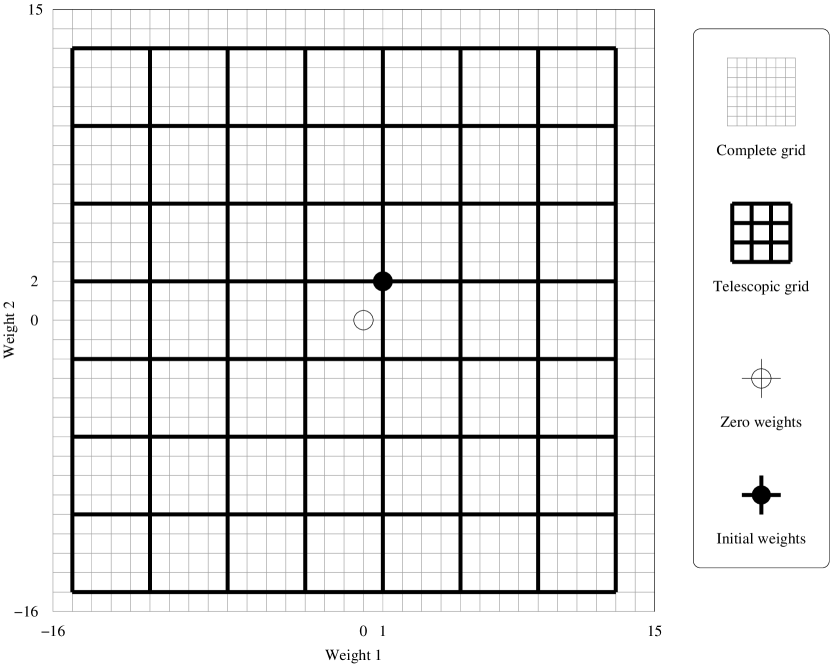
Figure 4: 2-weight network, $n=5$ bits per weight, initialized with small values (black dot). If only the $n^{\prime}=2$ most significant bits are changed, the accessible weight set (thick grid) does not include $(0,0)$.

III-F3 Initialization in telescopic BLM

Starting from small weights before running telescopic BLM requires a few considerations. Telescopic BLM initially operates on the most significant part of the weight representation, leaving the least significant bits untouched, thereby preventing any weight to return to zero until the final phase when it operates on all bits.
Fig. 4 shows the case where two $n=5$-bit weights are initialized with small values; for simplicity, the discretization step (1) has been set to $\epsilon=1$. If the initial step only involves the $n^{\prime}=2$ most significant bits, then the grid of actually accessible weight values is offset with respect to the origin, and weights are not allowed to vanish or, in some cases, even become smaller until later phases.
In some cases, the small offset acts as a beneficial noise source, forcing small random contributions and encouraging the use of spontaneous features, in the spirit of reservoir learning. Otherwise, it is possible to alleviate this problem by choosing random initial weights that are multiple of $\eta=2^{n-n^{\prime}}\epsilon$ (clearly, $w_{\text{init}}>\eta$, therefore initial weights are not going to be as small), so that all least significant bits are forced to zero.

In this paper, for lack of space, we concentrate mostly on the latest two options.

IV Tests on the two-spirals problem

The purpose of the experiments in this section is to test the effect of the BLM algorithm on a two-dimensional benchmark task, so that results can be visualized to develop some intuition before the second series of quantitative tests in the following sections.

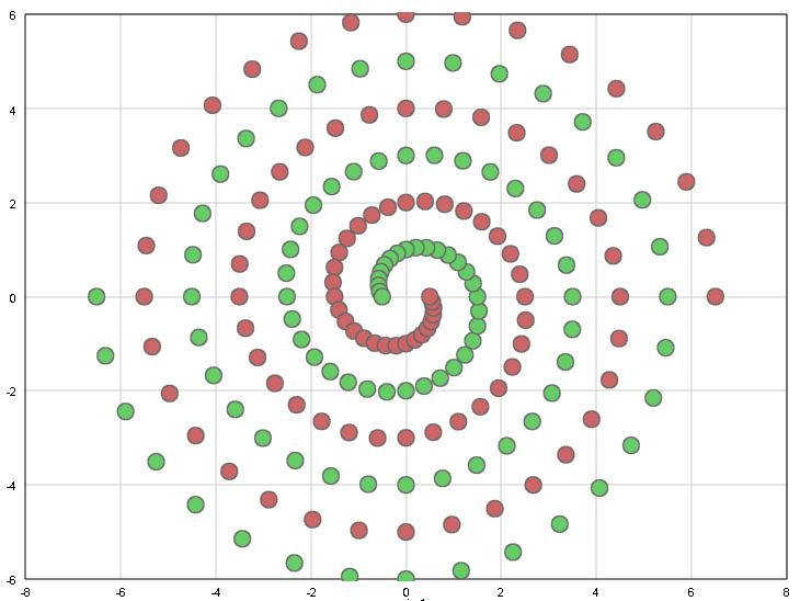
Figure 5: The two-spirals problem.

A highly nonlinear classification benchmark which is particularly difficult for gradient descent optimization is the “two spirals” problem developed in [20]. The data set is taken from the CMU Neural Networks Benchmarks. It consists of 193 training instances and 193 test instances located on a 2D surface. They belong to one of two spirals, as shown in Fig. 5

It is possible to solve this problem with one or two hidden layers, but architectures with two hidden layers need less connections and can learn faster. The architecture we consider here is $2-20-20-1$ with bias. The hidden units consist of symmetric sigmoids (hidden layers) and the usual $0-1$ sigmoid for the output unit. All points are used for training, the final mapping is shown with a contour plot for a visual representation of its generalization abilities.

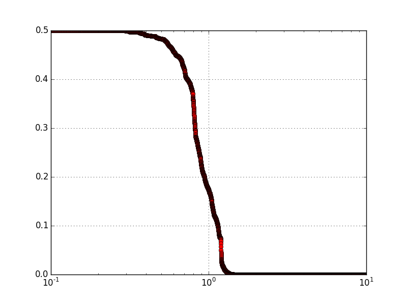
Figure 6: Two-spirals with OSS: RMS error as a function of CPU time. Log time axis.

Simple backpropagation tends to remain trapped in local minima or lead to excessive CPU times. The one-step secant (OSS) technique[21, 22] based on approximations of second derivatives from gradients is much more effective and is among the state-of-the-art methods for training this kind of highly nonlinear systems. The RMS error of OSS as a function of CPU time is shown in Fig. 6. It can be shown that a large number of OSS iterations (about 2000) are spent in the initial phase without significantly improving the RMS error, then the proper path in weight space is identified and the error rapidly goes to zero.

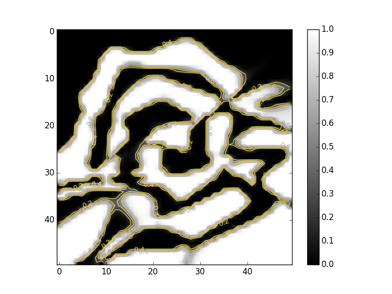
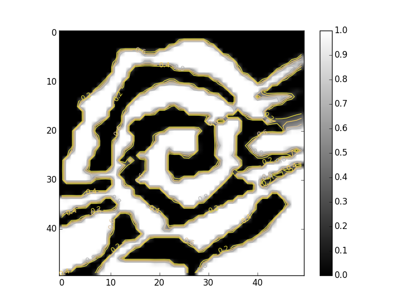
Figure 7: Two-spirals with OSS: intermediate result (above, 2000 iterations, RMS 0.02) and final map obtained.

The final results obtained with OSS are shown in Fig. 7. Some signs of over-training are clearly visible as stripes in the map. Early stopping does not help. Let’s focus on the final map for a fair comparison with those obtained by BLM at the local minimum.

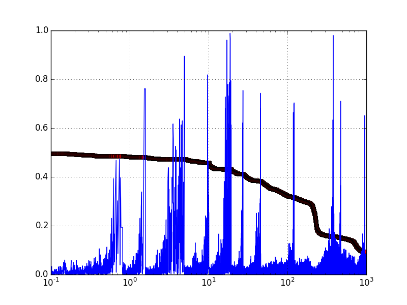
Figure 8: Two-spirals with telescopic BLM, 20-20 architecture, training RMSE as a function of CPU time, one curve (top, red) shows the RMSE evolution, the second curve (blue, bottom) shows the percentage of the neighborhood considered at each step.

Results for telescopic BLM are in Fig. 8 The architecture is the same as that used for OSS. The specific parameters of BLM are: initial weight range .001, initial number of bits 2, 12 bits, weight range 6.0.

It can be observed that the percentage of the neighborhood considered at each step is below 1% for most steps, with rare jumps up to 5-10% (these rare jumps are visible in the plot which shows all 726702 steps executed in 1000 seconds). The fraction of the neighborhood explored by first-improve tends to grow only in the final part of search for each number of bits, when the local minimum is close and more and more neighbors need to be examined before finding an improving move. After the local minimum is reached, a new bit is added to each weight so that the fraction drops again to very low values. Each macroscopic spike therefore corresponds to the moment when a local minimum is reached and the number of bits is increased.

The various local minima correspond to the mappings of Fig. 9. The telescopic “multi-scale” algorithm works by first modelling the overall large-scale circular structure and the south positive and north negative area. Then finer and finer internal details are fixed. The spiral maps is already well formed with 10 bits, while the two additional bits add some fine-tuning.

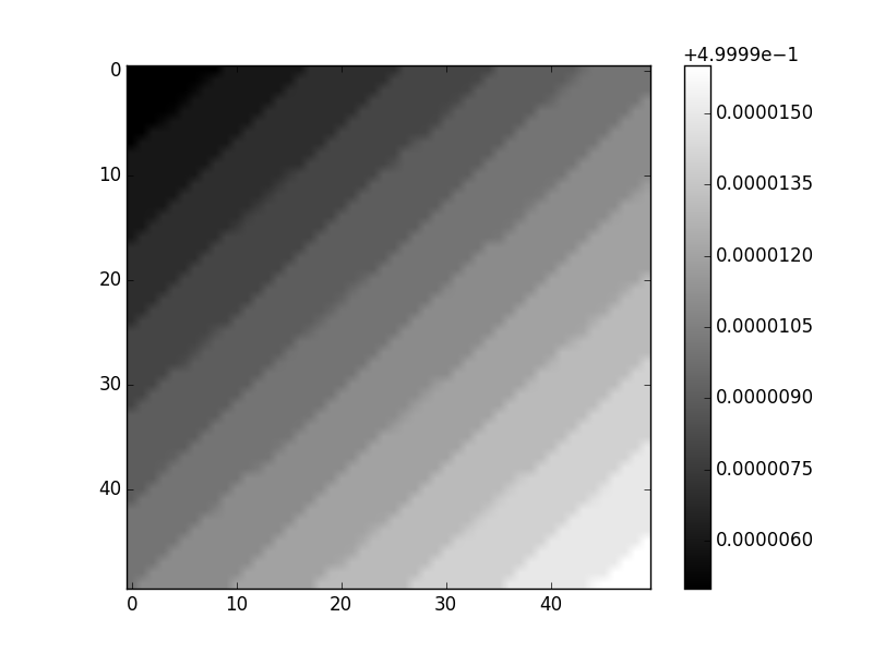
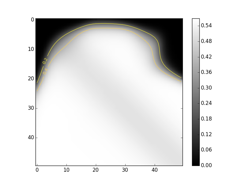
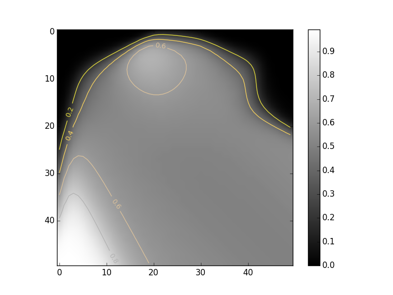
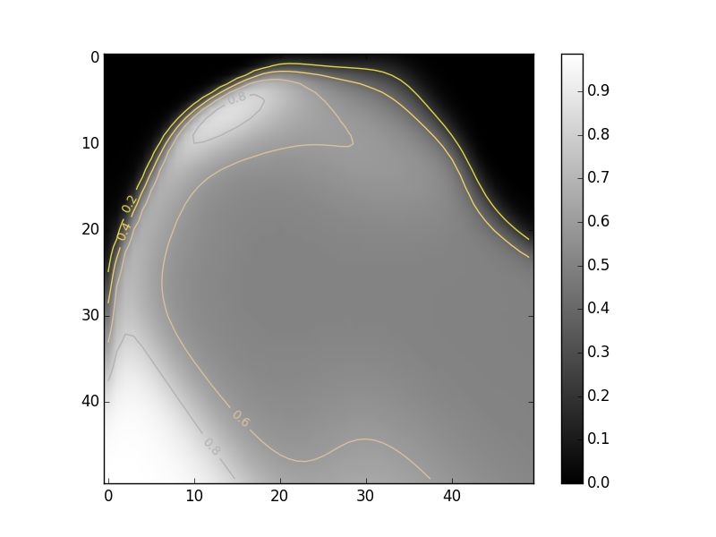
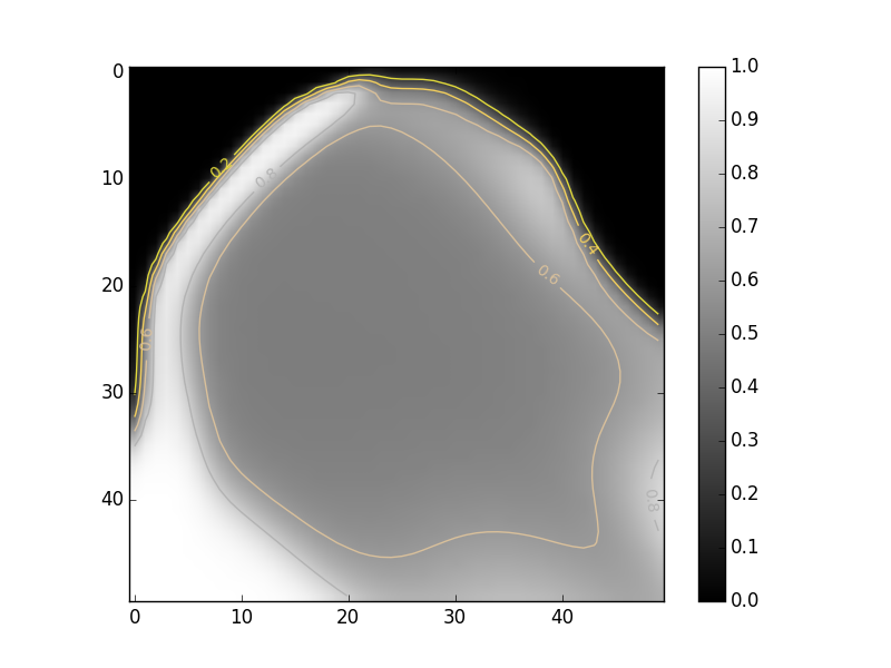
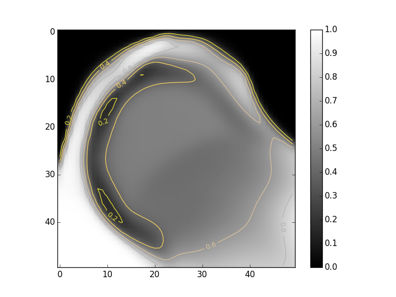
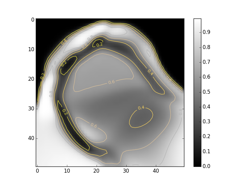
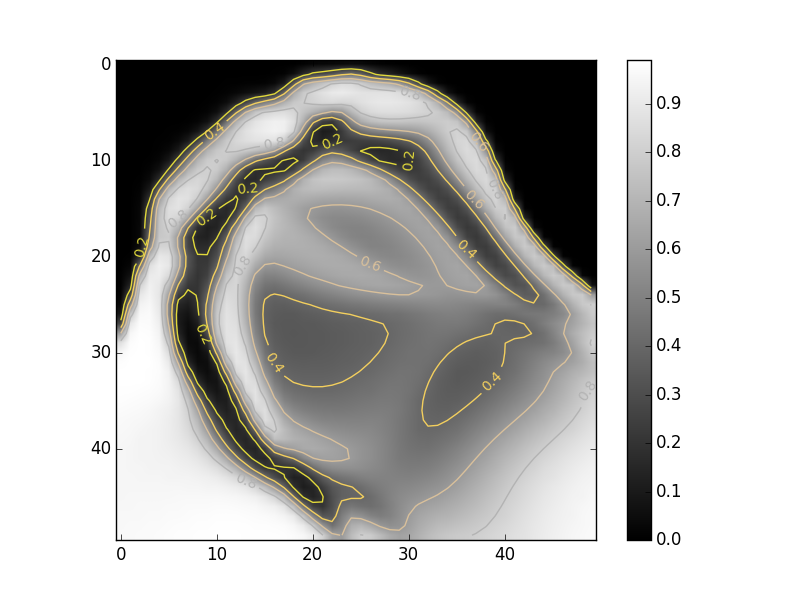
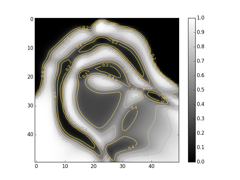
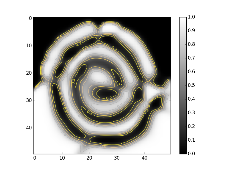
Figure 9: Two-spirals with telescopic BLM, 20-20 architecture. The capability of the map to represent the spiral increases when the number of bits per weight increases (from 1, top left, to 12, bottom right).

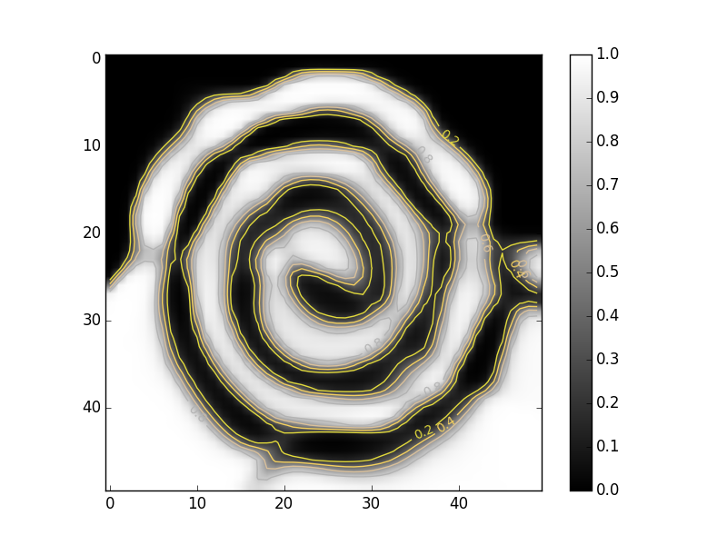
Figure 10: Two-spirals with telescopic BLM, 20-20 architecture, final mapping obtained.

The final mapping obtained (Fig. 10) is very smooth, without the signs of overtraining which are evident in the mapping for OSS. This result is surprising given that is is obtained with discretized weights represented with 12 bits.

Because BLM acts by local search changing individual bits, it is simple to consider variations of the algorithms. For example, sparsity can be encouraged, by aiming at networks in which a large number of weights is fixed to zero (and therefore can be eliminated from the final realization).

To encourage sparsity, in the following test only 50% of the weights are initialized with values different from zero, and the analysis of potential moves in the neighborhood at each step is changed as follows. First all bits in non-zero weights are tested for a possible change. Only of no such bit is identified, bits in zero weights are considered. The philosophy is “Let the current neurons fully express their potential before adding additional neurons (with non-zero weights)”.

The evolution of this sparsity-enforcing training is shown in Fig. 11. It can be observed that the final distribution of weights is indeed sparse (Fig. 12), with a peak at zero and two peaks at the smallest and largest possible values. The final mapping is smoother than the one obtained without enforcing sparsity (Fig. 13).

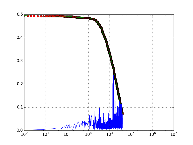
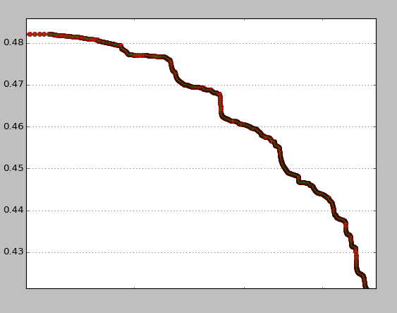
Figure 11: Two-spirals with sparsity enforcing, evolution of training (Circles: RMSE as a function of CPU time; line: fraction of explored neighborhood). Inset: zoom-in of the initial improvement; the step-like behavior is due to new neurons becoming active (new non-zero weights).

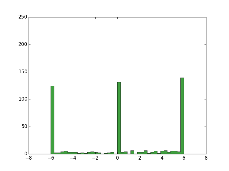
Figure 12: Two-spirals with sparsity enforcing, final distribution of weights.

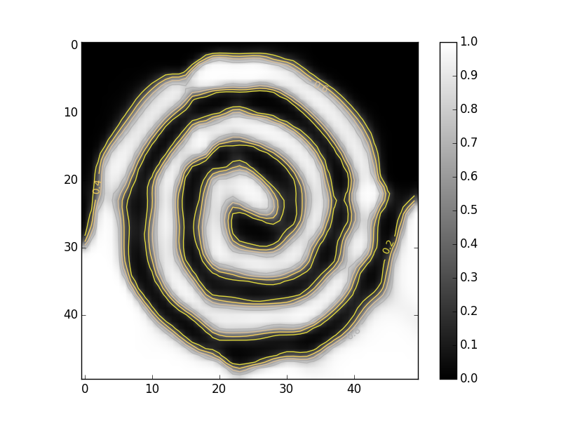
Figure 13: Two-spirals with sparsity enforcing, final mapping obtained.

While we have no space in this paper to investigate the sparsity issues for all benchmarks, the above preliminary results are encouraging and we plan to extend the analysis in future work.

V Tests on a control problem: the inverted pendulum

Figure 14: BLM-trained neural network as a controller.

In this Section we describe our investigation on the use of BLM-trained networks for applications in control problems, with the network acting as a controller component of a feedback loop, as shown in Fig. 14.

In the scheme, we can exploit the main advantage of BLM as a derivative-free training algorithm: the controlled physical system can be treated as a black box, with the only obvious addition of a system-specific error evaluation function (top right) whose numeric output measures the correctness of the system’s behavior.

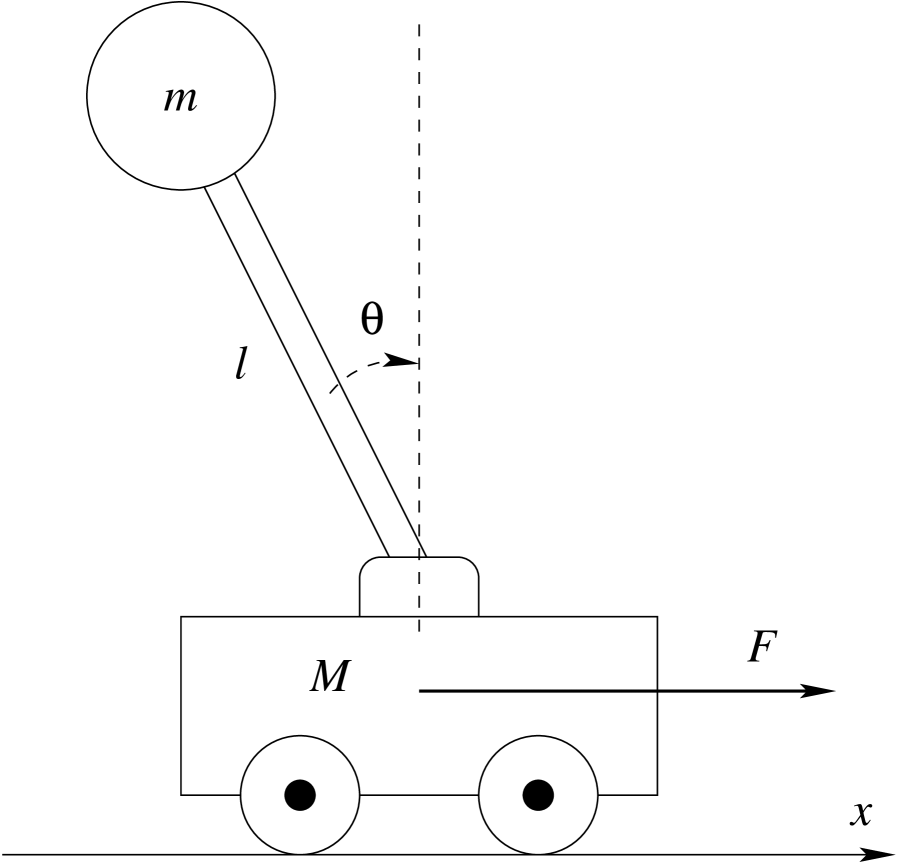
Parameters:
$M=m=1\text{kg}$,
$l=1\text{m}$.

Time discretization:
$t\in[0,100\text{s}]$,
$\Delta t=.01\text{s}$.

Initial conditions:
$x_{0}=0$,
$\theta_{0}\in[-.4,.4]$.

Figure 15: Inverted pendulum on a cart.

In our case study, we simulate the well-known system shown in Fig. 15: an inverted pendulum mounted on a cart on which a control force is applied. The cart has mass $M$ and is constrained to move along direction $x$, while the pendulum has length $l$ and mass $m$ applied on the end. Other masses are negligible. The control variable is a force applied to the cart along its moving direction.

The dynamics of the system are described by the following second-order, nonlinear system of differential equations:

$$\ddot{x} = \frac{F-m\sin\theta(l\dot{\theta}^{2}-g\cos\theta)}{M+m\sin^{2}\theta}$$

$$\ddot{\theta} = \frac{\ddot{x}\cos\theta+g\sin\theta}{l}.$$

The correct behavior of the system is to keep the pendulum in upright position $\theta=0$, with the cart at a specified coordinate $x=0$. If we simulate the system in the time interval $[0,T]$, then the error is given by a combination of the mean squares of the two position variables $x,\theta$:

$$\text{Err}(x,\theta)=\frac{1}{T-t_{\text{min}}}\int_{t_{\text{min}}}^{T}\left(\theta^{2}(t)+\lambda x^{2}(t)\right)\mathop{}\!\mathrm{d}t,$$ (7)

where $\lambda$ is a suitable weighting factor (in our experiments, $\lambda=0.01\text{m}^{-2}$), while $t_{\text{min}}\geq 0$ defines a transient portion of the time interval that does not contribute to the error.

V-A Complete feedback

In our first test, we use a feed-forward neural network with a 5-neuron hidden layer (with $\tanh$ as transfer function) and a single output neuron that provides the control force. The network has four inputs: the two position variables $x,\theta$ and their time derivatives $\dot{x},\dot{\theta}$. We use 16-bit weights, with $10$ as maximum value, initialized to small random values in the $[-10^{-2},10^{-2}]$ interval.

For the training procedure, we generate $50$ pendulum simulations, each running for a simulated time $T=100\text{s}$. We use first-order (Euler) integration with time increment $\Delta t=10^{-2}\text{s}$. The control force is kept constant for $10$ consecutive steps, after which the system’s status is fed to the neural net, and the new output is used for the subsequent 10 iterations. Therefore, the net is queried $1000$ times per simulation. The first $10$ network queries, corresponding to $t_{\text{min}}=1\text{s}$ of simulated time, don’t account for the error. Every $100$ training iterations, a different set of $50$ simulations is used to validate the training and the weights corresponding to the best validation are saved.

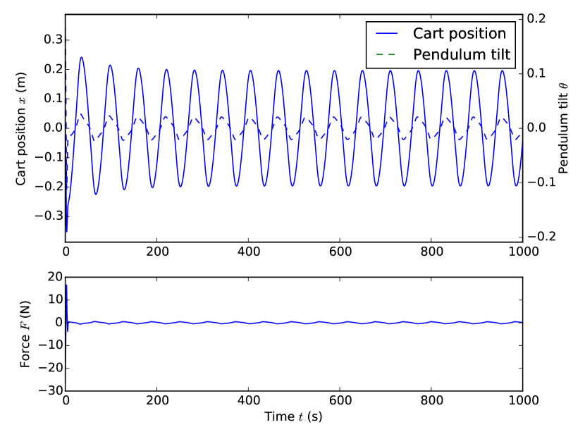
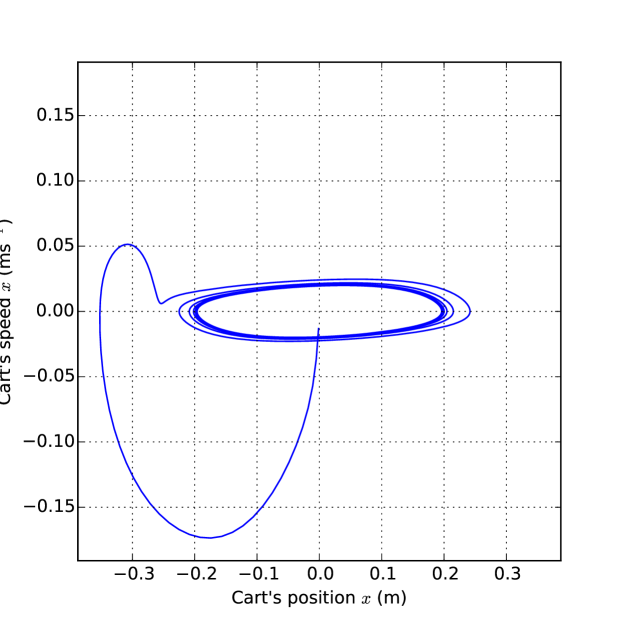
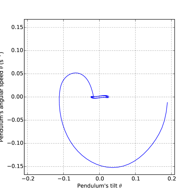
Figure 16: Inverted pendulum with complete feedback ($x,\theta,\dot{x},\dot{\theta}$), feed-forward MLP without recurrence, 5 hidden units and optimization on 2 bits per weight. Two bits are sufficient to keep the pendulum from falling, although control is coarse and both the pendulum and the cart keep moving back and forth along a limit cycle, as shown by the two phase-space diagrams in the bottom part.

Fig. 16 shows the behavior of a network with 5 hidden units trained with only 2 bits per weight on a sample test instance; to make sure that the stability is not temporary, the test simulation runs for $1000$ simulated seconds, i.e., tenfold the actual training and validation period. The top chart of Fig. 16 shows the behavior of the two positional variables $x,\theta$ during the simulation. The network’s control, however coarse due to the few representable weight values, is sufficiently precise to prevent the pendulum from falling, although the cart tends to drift back and forth (remember that we gave a relatively small value to the penalty $\lambda$ associated to the cart position $x$). The middle chart in the same Figure shows the corresponding applied force: after a transient high force to correct the unbalanced initial conditions of the system, much less force needs to be applied to keep the system upright. The ensuing periodicity is apparent in phase space, where the pairs of coordinates $(x,\dot{x})$ and $(\theta,\dot{\theta})$ both converge to a limit cycle. The mean error of the network as defined in (7), computed on $50$ random initial conditions, is $\text{Err}=2.34\cdot 10^{-2}$.

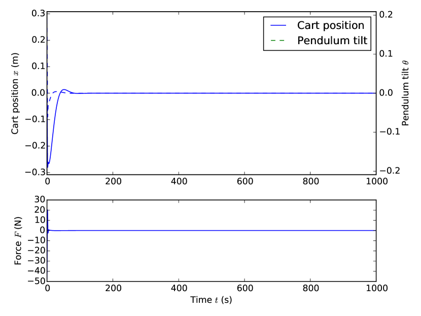
Figure 17: Inverted pendulum with complete feedback ($x,\theta,\dot{x},\dot{\theta}$), feed-forward MLP without recurrence, 5 hidden units and telescopic optimization on 16 bits per weight. The pendulum is now stabilized within a short time span.

If a finer representation is chosen for weights (e.g., 16 bits), then the system comes to a relatively smooth halt in a short time, as shown in Fig. 17, with error $\text{Err}=8.9\cdot 10^{-3}$.

V-B Derivative-free feedback

Moving to a harder version of the problem, we assume that only the positional variables $x,\theta$ are fed back to the network, while their time derivatives are not. The resulting network only has two inputs and one output.

In this case, a pure feed-forward network is unaware of the current inertial status, and the best that we can obtain is a slowly divergent system in which oscillations become larger and larger while the cart moves away from the central position.

The addition of recurrent connections from the hidden layer to itself, together with a convenient increase of the number of hidden units, provides the small amount of short-term memory that the network needs in order not to diverge.

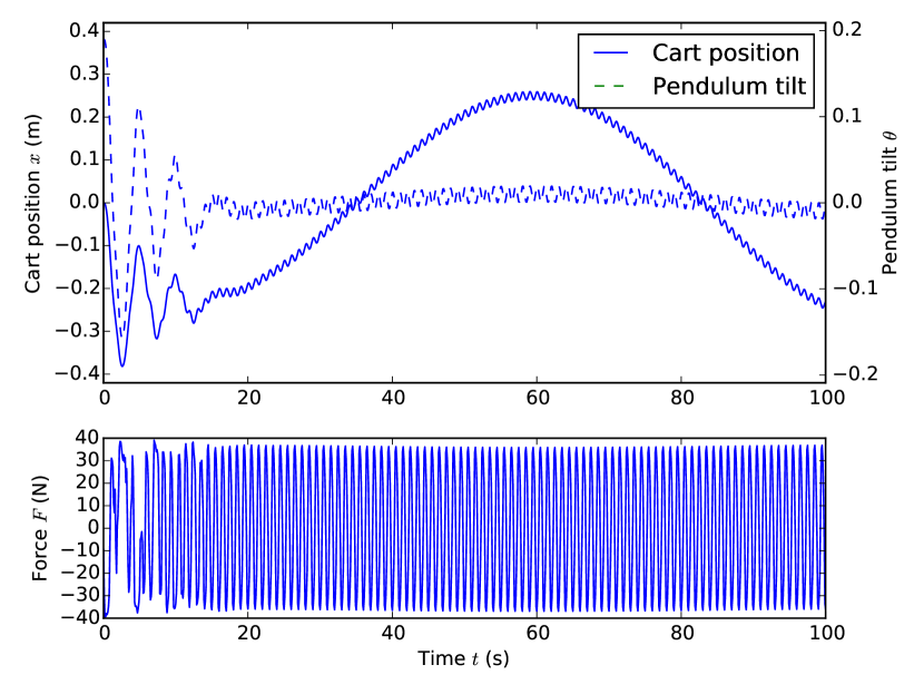
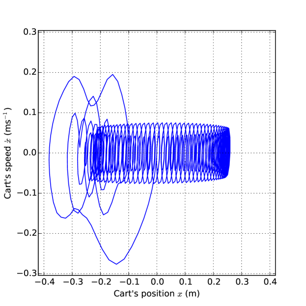
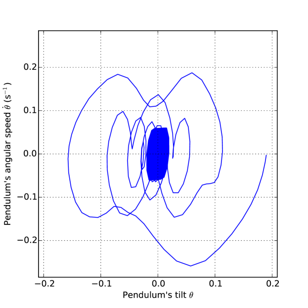
Figure 18: Inverted pendulum with derivative-free feedback ($x,\theta$), recurrent MLP with 20 hidden units and telescopic optimization on 16 bits per weight. Top: evolution of the positional variables in time; middle: network output (force applied to the cart); bottom: phase-space diagrams. Only the initial $100\text{s}$ of simulated time are shown for clarity.

Fig. 18 shows the behavior of the system when controlled by a recurrent network with 10 hidden units trained with the same parameters as before. The control variable output by the neural net is quite jittery, possibly due to time discretization, but the resulting system can keep track of its current status and maintain the pendulum close to the upright position, while keeping the cart in proximity to the central position. The cart keeps its equilibrium throughout the $1000$-second simulation, but only the initial $100\text{s}$ are shown for clarity. The limit cycles tend to drift back and forth, therefore they don’t clearly appear in the two bottom phase-space diagrams. Although the dynamics look quite different, the overall error is kept low by the lower variability of the pendulum tilt: $\text{Err}=2.28\cdot 10^{-2}$.

V-C Convergence to suboptimal attractors

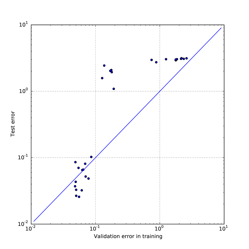
Figure 19: Distribution of validation and test results for a derivative-free instance of the inverted pendulum problem. Test instances have a longer simulated time, therefore tend to have extreme outcomes.

While training recurrent networks on the derivative-free version, the existence of suboptimal attractors becomes apparent. We performed 30 independent training sessions on networks with 10 hidden units and 16 bits per weight. The telescopic method was used, starting from 2 bits, and increasing the number of bits whenever the estimated ratio of improving moves falls below $\phi=10\%$, estimated by means of the technique described in Sec. III-E2 with a mobile average decay factor $\eta=.95$. Fig. 19 shows a scatterplot of the best validation error obtained during training versus the test error computed with a fresh set of examples and a longer simulated time. While about half of the tests is concentrated in the low-error area ($Err<.1$), the other half converges to configurations with much higher errors, which are amplified by the longer testing times.

Observe that test errors tend to be much more polarized (almost no values in $[0.1,1]$) than the corresponding validation errors. This is due to the fact that test error are executed for a longer simulated timespan ($1000\text{s}$ vs. $100\text{s}$), while training and validation instances are kept shorter in order to speed up the training phase.

TABLE I: Convergence to suboptimal attractors in the inverted pendulum derivative-free case (30 samples)

Hidden	Test error			Median time
units	Minimum	1st quartile	# less than $.1$	(seconds)
5	1.205	1.205	0 / 30	42
10	0.023	0.130	7 / 30	97
20	0.037	0.052	13 / 30	222
40	0.028	0.382	4 / 30	568

The non-negligible ratio of suboptimal attractors can be avoided by simply repeating the optimization until the desired error level is attained. As shown in Tab. I, in fact, apart from the smaller 5-unit network, all network sizes were able to attain low errors in at least some of the 30 training sessions. In the 20-unit network, 13 runs out of 30 ended with a low error: the probability of finding a good result after $N$ restarts is thus $1-(17/30)^{N}$, and the expected time to obtain a low error configuration is $222\text{s}\cdot(30/13)\approx 512\text{s}$.

VI Additional tests on feed-forward networks

TABLE II: Specification of the 4 benchmark sets used in comparisons

Dataset name	Training samples	Test samples	Attributes	Outputs
house16H	15948	6836	$16$	1
yeast	1038	446	$8$	10 (classif.)
abalone	2924	1253	$7+1$	1

In the following we collect experimental results on the widely used benchmark real-life regression and classification problems listed in Table II. The datasets have been chosen among the larger ones presented in [23].

The house16H dataset contains housing information that relates demographics and housing market state of a region with the median price of houses.

The yeast dataset consists of a classification problem. The task is to determine the localization site of protein in gram-negative bacteria and eukaryotic cells [24, 25]. Output is coded with a unary representation (1 for the correct class, 0 for the wrong classes). In addition to the traditional RMSE error, also the cross-entropy (CE) error is considered in this classification case.

The abalone dataset contains data on specimens of the Abalone mollusk; 7 columns report physical measures, one column is nominal (male/female/infant), and for our purposes it has been transformed into three $\pm 1$-valued inputs, so that a total of 10 inputs were used. The output column is the age of the specimen (number of accretion rings in the shell).

All dataset inputs have been normalized by an affine mapping of the training set inputs onto the $[-1,1]$ range and by an affine mapping of the outputs onto the $[0,1]$ range. The affine normalization coefficients obtained on the training set have also been applied to the test set values. 70% of the examples are used for training, 30% for validation. Given that we did not repeat the experiments to determine free parameters, a separate test set was not deemed necessary (the terms validation and test are used with the same meaning in the following description).

VI-A House benchmark

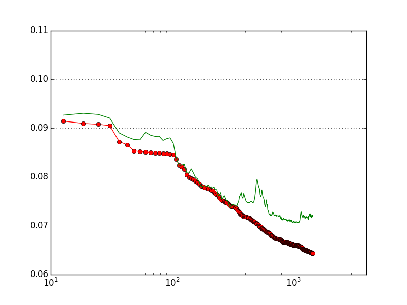
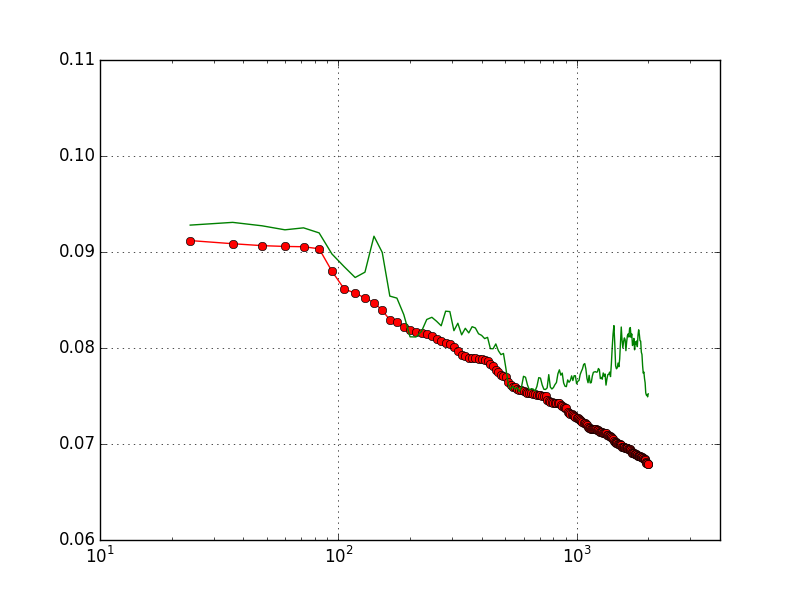
Figure 20: OSS for house: training and validation data as a function of CPU time. 100 hidden units (above), 200 hidden (below). Average RMS error on training set (circles) and on test set (simple line).

Before analyzing the distribution of results over multiple runs, it is of interest to observe two individual runs of OSS and BLM for 100 and 200 hidden units. The transfer functions are symmetric sigmoid (hidden units) and linear (output units). Weights are initialized randomly in the range (-0.01,0.01). For BLM, the number of bits is 12, and the weight range 8.0. BLM regularization weight is 1.0. The runs last 4000 seconds.

In Fig.20 one observes a qualitative difference: While the error on the training set always decreases (as expected), the generalization error on the validation set has a noisy and irregular behavior for OSS, with clear signs of overtraining at the end of the run. The evolution of the validation error for BLM is much smoother and no sign of over-training is present. We conjecture that this behavior is caused by the more stochastic (less “greedy”) choice of each weight change in BLM with respect to OSS. The best validation results are generally better for BLM (with improvements of around 1-3%).

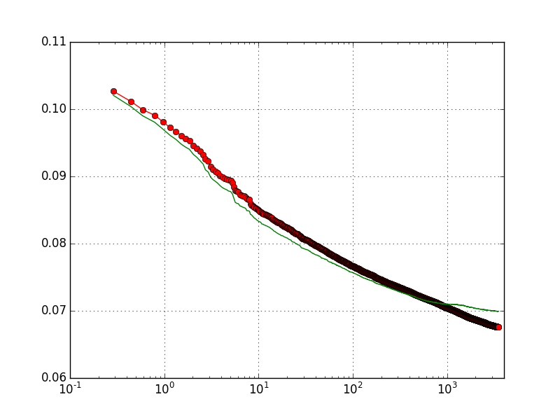
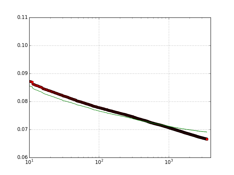
Figure 21: BLM (non-telescopic) for house: training and validation data. 100 hidden (above) 200 hidden (below). Average RMS error on training set (circles) and on test set (simple line).

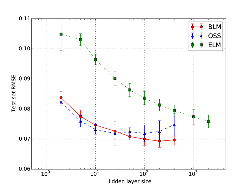
Figure 22: House benchmark. Validation results as a function of hidden layer size.

The results of five runs for each configuration, with different numbers of hidden neurons, are plotted in Fig. 22 with error bars (estimated error on the average). The test results of BLM are better than those of OSS, in particular for large networks, a result which confirms less over-training for BLM. For 400 hidden units, results are 7% better for BLM. ELM needs a very large number of hidden units to obtain competitive results, but the error for 4000 hidden nodes (0.0758) is still 10% worse than the best BLM results.

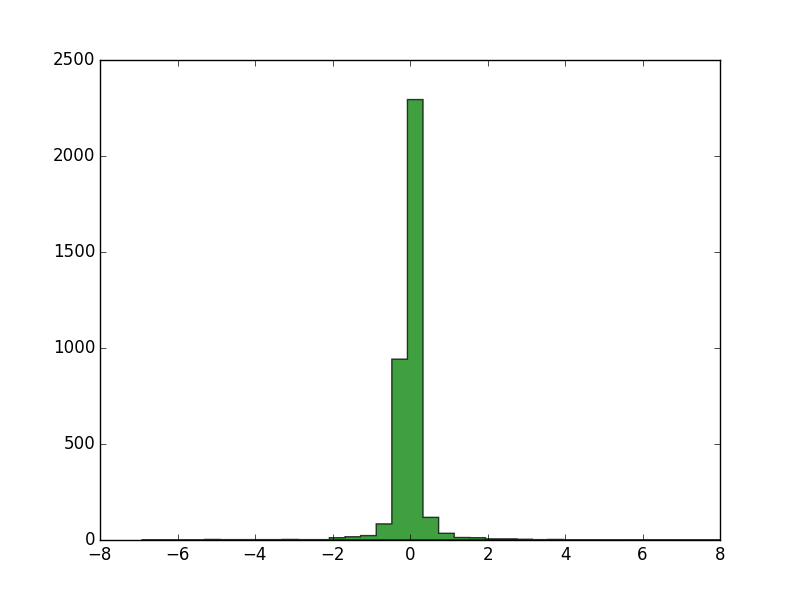
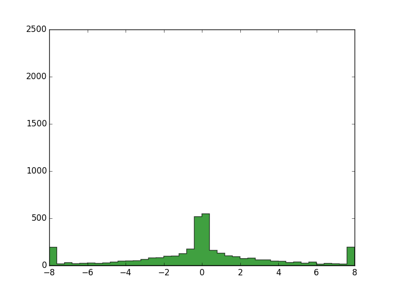
Figure 23: House benchmark. Distribution of weight values (200 hidden units). OSS (above) BLM (below).

In order to understand if the difference in validation is related to the final size of weights, the final distribution of weights is shown in Fig. 23. The histogram shows that the better generalization for BLM cannot be explained in a simple manner by a smaller average weight magnitude, which actually tends to be larger for BLM. There is evidence that the search trajectory in weight space of BLM explores parts which are not explored by the more “greedy” OSS based on gradient descent.

VI-B Yeast benchmark

The yeast benchmark task is a classification problem. With our unary output encoding (1 for the correct class, 0 otherwise), at least two error measures are of interest, the RMS error and the cross-entropy (CE) error. The second better reflects the classification nature of the task, but the first is also reported for uniformity with the other benchmarks considered in this paper.

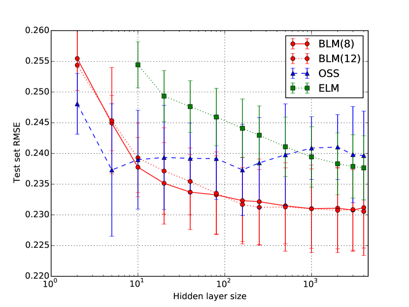
Figure 24: Yeast benchmark (RMS error). Validation results as a function of hidden layer size. BLM with maximum weight range 8.0 (BLM(8)) and 12.0 (BLM(12)), ELM, and OSS.

The parameters of the runs are: symmetric sigmoid (hidden layer), standard 0-1 sigmoid (output layer). Initial weigh range 0.001, two values for the weight range in BLM (8 and 12). The runs last 500 seconds. The RMSE validation results (Fig. 24) as a function of the number of hidden nodes show superior results by BLM. OSS obtains close results for small numbers of hidden units but shows a larger standard deviation. ELM needs a very large hidden layer to reach result of interest. For a quantitative comparison, the best average validation results are of for 0.231 BLM, of 0.237 for OSS, of 0.238 for ELM.

The two plots for the different weight range (8 and 12) for BLM show that the detailed choice of this parameter is not critical (a value between 6 and 12 usually corresponds to a plateau of best results).

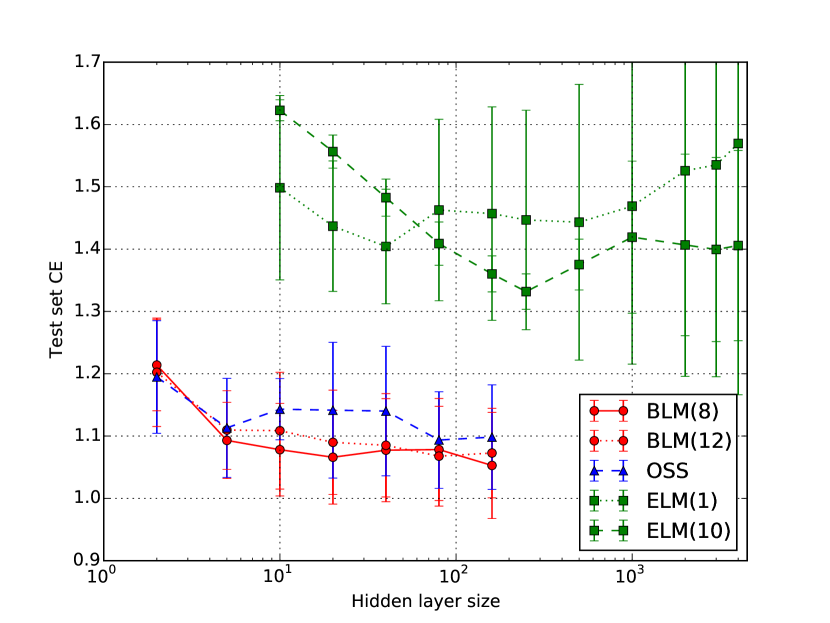
Figure 25: Yeast benchmark (CE error). Validation results as a function of hidden layer size. BLM with maximum weight range 8.0 (BLM(8)) and 12.0 (BLM(12)), ELM with regularization parameter 1 (ELM(1), with regularization parameter 10 (ELM(10)), and OSS.

The results for the cross-entropy error (Fig. 25) show similar validation results for OSS and BLM, and inferior results for ELM. In an attempt to improve BLM results, different values of the regularization parameter (from 0.1 to 100) have been tested. Two plots for values 1 and 10 are shown. The parameter does influence the results but they remain in any case far from those of BLM and OSS.

VI-C Abalone benchmark

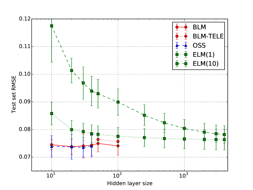
Figure 26: Abalone benchmark (RMS error). Validation results as a function of hidden layer size. BLM with maximum weight range 8, Telescopic BLM, ELM with regularization parameter 1 (ELM(1), with regularization parameter 10 (ELM(10)), and OSS.

The parameters of the runs are: symmetric sigmoid (hidden layer), linear (output layer). Initial weigh range 0.001, two values for the regularization parameter of BLM (1 and 10). For BLM, both the telescopic and the normal version are compared. The runs last 500 seconds.

The average RMS error on validation for different numbers of neurons in the hidden layer is shown in Fig. 26. One can observe that OSS and BLM results are similar. Results of normal or telescopic BLM are almost indistinguishable. As usual, ELM needs a fat hidden layer to reach competitive results, but results with 4000 hidden units are still larger than those of OSS/BLM.

VII Conclusions

The objective of this paper was not that of proposing yet another technique but that of revisiting basic stochastic local search to assess the baseline performance of algorithmic building blocks in order to motivate more complex methods. Better said, the algorithm considered from the point of view of discrete dynamical systems in the weight space is simple; complexity is delegated to the implementation with the design of efficient methods and data structures to enormously reduce CPU times.

The results were counterintuitive. In the considered benchmark cases our Telescopic BLM algorithm not only reproduced results obtained by more complex methods, but actually surpassed them by a statistically significant gap in some cases. Also the performance produced by extreme learning was improved, in some cases with much smaller networks (with a smaller number of hidden units). To be fair, let’s note that ELM is extremely fast and better than simple back-propagation and therefore should not be discounted as a promising technique.

The experimental results indicate that a simple method like BLM based on stochastic local search and an adaptive setting of the number of bits per weight is fully competitive with more complex approaches based on derivatives or based only on function evaluations.

The speedup obtained by supporting data structures, incremental evaluations, a small and adaptive number of bits per weight, and stochastic first-improvement neighborhood explorations is of about two orders of magnitude for the benchmark problems considered, and it increases with the network dimension. The CPU training time is still much larger than that obtained by ELM via pseudo-inverse, but still acceptable if the application area does not require very fast online training.

We feel that the interesting results obtained will motivate a wider application of BLM for more complex networks and machine learning schemes, and we are continuing the investigation in this direction. We encourage researchers to consider special-purpose hardware implementations, or realizations on GPU accelerators. Ensembling is another promising avenue [26], as well as the theoretical analysis of the dynamics in weight space produced by Telescopic BLM.

References

- [1] P. Werbos, “Beyond regression: New tools for prediction and analysis in the behavioral sciences,” Ph.D. dissertation, Harvard University, Cambridge, MA, 1974.
- [2] D. Rumelhart, G. Hinton, and R. Williams, “Learning internal representations by error propagation,” in Parallel Distributed Processing: Explorations in the Microstructure of Cognition. Vol. 1: Foundations, D. Rumelhart and J. L. McClelland, Eds. MIT Press, 1986.
- [3] C. Cortes and V. N. Vapnik, “Support vector networks,” Machine Learning, vol. 20, no. 3, pp. 1–25, Sep 1995.
- [4] G.-B. Huang, Q.-Y. Zhu, and C.-K. Siew, “Extreme learning machine: theory and applications,” Neurocomputing, vol. 70, no. 1, pp. 489–501, 2006.
- [5] M. Lukoševičius and H. Jaeger, “Reservoir computing approaches to recurrent neural network training,” Computer Science Review, vol. 3, no. 3, pp. 127–149, 2009.
- [6] R. S. Sexton, R. E. Dorsey, and J. D. Johnson, “Optimization of neural networks: A comparative analysis of the genetic algorithm and simulated annealing,” European Journal of Operational Research, vol. 114, no. 3, pp. 589–601, 1999.
- [7] R. Hooke and T. A. Jeeves, ““direct search”solution of numerical and statistical problems,” Journal of the ACM (JACM), vol. 8, no. 2, pp. 212–229, 1961.
- [8] A. Corana, M. Marchesi, C. Martini, and S. Ridella, “Minimizing multimodal functions of continuous variables with the simulated annealing algorithm,” ACM Transactions on Mathematical Software (TOMS), vol. 13, no. 3, pp. 262–280, 1987.
- [9] R. Battiti and G. Tecchiolli, “Training neural nets with the reactive tabu search,” IEEE Transactions on Neural Networks, vol. 6, no. 5, pp. 1185–1200, 1995.
- [10] P. L. Barlett and T. Downs, “Using random weights to train multilayer networks of hard-limiting units,” IEEE Transactions on Neural Networks, vol. 3, no. 2, pp. 202–210, 1992.
- [11] M. Brunato and R. Battiti, “Stochastic local search for direct training of threshold networks,” in Proc. 2015 International Joint Conference on Neural Networks, in press, 2015.
- [12] H. H. Hoos and T. Stuetzle, Stochastic Local Search: Foundations and Applications. Morgan Kaufmann, 2005.
- [13] R. Battiti, M. Brunato, and F. Mascia, Reactive Search and Intelligent Optimization, ser. Operations research/Computer Science Interfaces. Springer Verlag, 2008, vol. 45.
- [14] R. Battiti and M. Brunato, The LION way. Machine Learning plus Intelligent Optimization. LIONlab, University of Trento, Italy, 2014.
- [15] S. Kirkpatrick, C. D. G. Jr., and M. P. Vecchi, “Optimization by simulated annealing,” Science, vol. 220, pp. 671–680, 1983.
- [16] P. J. M. Laarhoven and E. H. L. Aarts, Eds., Simulated annealing: theory and applications. Norwell, MA, USA: Kluwer Academic Publishers, 1987.
- [17] J.-L. Starck, F. D. Murtagh, and A. Bijaoui, Image processing and data analysis: the multiscale approach. Cambridge University Press, 1998.
- [18] E. Weinan and B. Engquist, “Multiscale modeling and computation,” Notices of the AMS, vol. 50, no. 9, pp. 1062–1070, 2003.
- [19] E. Mjolsness, C. D. Garrett, and W. L. Miranker, “Multiscale optimization in neural nets,” IEEE Transactions on Neural Networks, vol. 2, no. 2, pp. 263–274, 1991.
- [20] K. J. Lang, “Learning to tell two spirals apart,” in Proc. of 1988 Connectionist Models Summer School, 1988.
- [21] R. Battiti, “First-and second-order methods for learning: Between steepest descent and newton’s method,” Neural Computation, vol. 4, pp. 141–166, 1992.
- [22] R. Battiti and G. Tecchiolli, “Learning with first, second, and no derivatives: a case study in high energy physics,” Neurocomputing, vol. 6, pp. 181–206, 1994.
- [23] G.-B. Huang, Q.-Y. Zhu, K. Mao, C.-K. Siew, P. Saratchandran, and N. Sundararajan, “Can threshold networks be trained directly?” IEEE Transactions on Circuits and Systems II: Express Briefs, vol. 53, no. 3, pp. 187–191, 2006.
- [24] K. Nakai and M. Kanehisa, “Expert system for predicting protein localization sites in gram-negative bacteria,” Proteins: Structure, Function, and Bioinformatics, vol. 11, no. 2, pp. 95–110, 1991.
- [25] ——, “A knowledge base for predicting protein localization sites in eukaryotic cells,” Genomics, vol. 14, no. 4, pp. 897–911, 1992.
- [26] H. Chen, H. Chen, X. Nian, and P. Liu, “Ensembling extreme learning machines,” in Advances in Neural Networks–ISNN 2007. Springer, 2007, pp. 1069–1076.