Melnikov chaos in a modified Rayleigh-Duffing oscillator with $\phi^{6}$ potential

Abstract

The chaotic behavior of the modified Rayleigh-Duffing oscillator with $\phi^{6}$ potential and external excitation which modeles ship rolling motions are investigated both analytically and numerically. Melnikov method is applied and the conditions for the existence of homoclinic and heteroclinic chaos are obtained. The effects of nonlinear damping on roll motion of ships are analyzed in detail. As it is known, nonlinear roll damping is a very important parameter in estimating ship reponses. The predictions are tested numerical simulations based on the basin of attraction. We conclude that certains quadratic damping effects are contrary to cubic damping effect.

Institut de Mathématiques et de Sciences Physiques, Université d’Abomey-Calavi, BP: 613 Porto Novo, Bénin

keywords Modified Rayleigh-Duffing oscillator, Melnikov criterion, nonlinear damping effect, ship rolling, basin of attraction

1 Introduction

The analysis of nonlinear dynamic systems is now a major theme in both academic and industrial perspective and touches many areas, such as hydrodynamics, aerospace, civil engineering, transport, musical acoustics, nuclear engineering and others [Enjieu Kadji and Nana Nbendjo, 2012; Hayashi, 1964; Nana Nbendjo et al., 2007; Nayfeh and Mook, 1979; Tchoukuegno, 2002; Tchoukuegno, 2003; Yamapi, 2003; Yamapi, 2007]. The first works date from the nineteenth century including Poincaré, but currently it is experiencing a resurgence of interest due to the need to optimize, streamline structures commonly used and subjected to significant levels of excitement, or control the instabilities oscillations. Modeling and study of the behavior of a physical system is a major problem even complicated in case the present system nonlinearities. Much of the discussion in the physics and engineering literature concerning damped oscillations, focuses on systems subject to viscous damping, that is, damping proportional to the velocity, even though viscous damping occurs rarely in physical systems. Phenomenological models describing some type of nonlinear dissipation have been used in some applied sciences such as ship dynamics [Bikdash et al., 1994; Falzarano et al., 1992], where a particular interest has deserved the role played by different damping mechanisms in the formulation of ship stability criteria, and vibration engineering [Ravindra and Mallik, 1994a; Ravindra and Mallik, 1994b]. Damping in certain applied systems plays an important role, since it may be used to suppress large amplitude oscillations or various instabilities, and it can be also used

as a control mechanism [Litak et al., 2009; Miwadinou et al., 2015; Rand et al., 2000; Sanjuán, 1999; Soliman and Thompson, 1992, Taylan, 2000].

This paper is concerned with the appearance of homoclinic and heteroclinic instabilities and chaos in a triple-well modified Rayleigh-Duffing oscillator. Many problems in physics, chemistry, biology, Engineering, etc., are related Rayleigh-Duffing oscillator. [Miwadinou et al., 2014; Miwadinou et al., 2015; Siewe Siewe et al., 2009]. The dynamics of Rayleigh-Duffing oscillator has been investigated widely in these years [Miwadinou,]. For example, in their work, Siewe Siewe et al. [2006] studied the nonlinear response and suppression of chaos by weak harmonic perturbation inside a triple well $\phi^{6}-$Rayleigh oscillator combined to parametric excitations. In [Siewe Siewe et al., 2009], the authors focussed their analysis on the occurrence of chaos in a parametrically driven extended Rayleigh oscillator with three-well potential modeled by:

$$\ddot{x}-\mu(1-\dot{x}^{2})\dot{x}+(1-\gamma\cos\omega t)(x+\alpha x^{3}+\beta x^{5})=F\cos\omega t.$$ (1)

On the other hand, the Rayleigh-Duffing oscillator is used to model the roll motion of ships. The nonlinear ship rolling response generally is given by [Francescutto and Contento, 1999; Holappa et al., 1999; Scolan, 1999; Taylan, 2000]

$$\ddot{x}+2\mu\dot{x}+\beta_{1}|x|\dot{x}+\beta_{2}\dot{x}|\dot{x}|+\delta_{1}x^{2}\dot{x}+\delta_{2}\dot{x}^{3}++...+\omega_{0}^{2}x+a_{3}x^{3}+a_{5}x^{5}+$$ (2)

$$...=F\cos\omega t,$$ (3)

where $\omega_{0}$ and $\omega$ are internal and external frequencies respectively; $\mu$, $\beta_{i}$ and $\delta_{i}$ are linear, quadratic nonlinear and cubic nonlinear damping coefficients respectively and $a_{i}$ are restoring coefficients. $F$ is the external excitation amplitude. In these cases, Francescutto and Contento [1999] used experimental results and parameter identification technique to study bifurcations in ship rolling modeled as :

$$\ddot{x}+2\mu\dot{x}+\delta_{2}\dot{x}^{3}+\omega_{0}^{2}x+\sum_{j=1}^{11}a_{j}x^{j}=F\cos\omega t.$$ (4)

Scolan [1999] applied the Melnikov method to nonlinear ship rolling in waves modeled by

$$\ddot{x}+2\mu\dot{x}-x(x^{2}-x_{v}^{2})(x^{2}-x_{l}^{2})=A\cos(\omega t+\phi).$$ (5)

The author provided that the heteroclinic orbits still exist whatever the “smallness” of the perturbation as soon as the system is undamped. The existence of such cancellation is otherwise confirmed from an analysis of the erosion of the attraction basin. Application of the extended Melnikov’s method is used by Wan and Leigh [2008] for simple single-degree-of-freedom vessel roll motion. In their paper, the authors considered the two following ship rolling models:

$$\ddot{x}+\delta_{1}\dot{x}+\epsilon\delta_{2}\dot{x}|\dot{x}|+x-\alpha x^{3}=\epsilon f\cos\omega t,$$ (6)

$$\ddot{x}+\beta\dot{x}+x(1-x)(1+ax)=F\sin\omega t.$$ (7)

The authors compared their results with those obtained by Falzarano [1990] and Spyrou et al. [2002]. Our aim is to make a contribution to the study of the transition to chaos in the modified Rayleigh-Duffing oscillator with three well potential possessing both homoclinic and heteroclinic orbit by using Melnikov’s theory, and then see how the fractal basin boundaries arise and are modified as the damping coefficient is varied. We also focus our attention on the numerical investigation of the strange attractor at parameter values close to the analytically predicted bifurcation curves.

The paper is organized as follows. In Section 2, we describe and analyze the model. Section 3 deals with the conditions of existence of Melnikov’s chaos resulting from the homoclinic and heteroclinic bifurcation. In Section 4, the basins of attraction of the initial conditions are droped to verify the effectiveness of the method. We provided a conclusion and summary in the last section.

2 Description of the model

We examine the dynamical transitions in periodically forced self-oscillating systems containing the cubic and quintic terms in the restoring force; pure, hybrid quadratic and cubic terms in nonlinear damping function as follows:

$$\ddot{x}+\mu(1-\dot{x}^{2})\dot{x}+\beta\dot{x}^{2}+k_{1}\dot{x}x+x+\lambda x^{3}+\delta x^{5}=F_{0}\cos\omega t,$$ (8)

where $\mu,\beta,k_{1},\lambda,\delta,F_{0}$ and $\omega$ are parameters. Physically, $\mu,\beta$ and $k_{1}$ represent respectively pure cubic and pure, unpure quadratic nonlinear damping coefficient terms; $\omega$ and $F_{0}$ are respectively the frequency and the amplitude of external periodic forcing. Moreover $\lambda$ and $\delta$ characterizes the intensity of the nonlinearity and $\epsilon$ is the nonlinear damping control parameter. The nonlinear damping term corresponds to the modified Rayleigh oscillator, while the nonlinear restoring force corresponds to the Duffing oscillator, hence the oscillateur is the so-called three-well potential modified Rayleigh-Duffing oscillator.

We derive the fixed points and the phase portrait corresponding to the system (Eq. (8)) when this is unperturbed. Eq. (8) becomes an unperturbed system and can be rewritten as

$$\dot{x}=y,\quad\dot{y}=-x-\lambda x^{3}-\delta x^{5},$$ (9)

which corresponds to an integrable Hamiltonian system with the potential function given by

$$V(x)=\frac{1}{2}x^{2}+\frac{1}{4}\lambda x^{4}+\frac{1}{6}\delta x^{6},$$ (10)

whose associated Hamiltonian function is

$$H(x,y)=\frac{1}{2}y^{2}+\frac{1}{2}x^{2}+\frac{1}{4}\lambda x^{4}+\frac{1}{6}\delta x^{6}.$$ (11)

From Eqs. (9) and (11), we can compute the fixed points and analyze their stabilities.

$\bullet$ If $\lambda^{2}<4\delta$, the unperturbed system has only fixed point $(0,0)$ which is a center and the potential $V$ has single well (see Fig. 1 ).

$\bullet$ For $\lambda^{2}=4\delta$ with $\lambda>0$ and $\delta<0$, the unperturbed system has three fixed points: two saddles connected by two heteroclinic orbits and one center.

$\bullet$ For $\lambda^{2}>4\delta$ with $\lambda<0$ and $\delta>0$, the unperturbed system has five fixed points: two saddles connected by two heteroclinic orbits, and the two saddle points are connected to themselves by one homoclinic orbit. The system has three centers and the potential defined by Eq. (10) has three-well (see Fig. 2 ).

In this paper, we consider the first and third cases. We set $\lambda=0.3$, $\delta=-0.08$ and $\lambda=-0.6$, $\delta=0.05$ respectively in single-well potential and three-well potential cases.

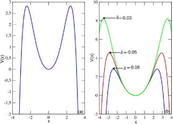
Figure 1: $(a):$ Single-well potential of the unperturbed system; $(b):$ Shape of single-well potential for different values of $\delta$.

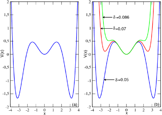
Figure 2: $(a):$ Triple well potential of the unperturbed system; $(b):$ Shape of triple well potential for different values of $\delta$.

3 Melnikov analysis

In this section, we discuss the chaotic behavior of the system

$$\ddot{x}+\mu(1-\dot{x}^{2})\dot{x}+\beta\dot{x}^{2}+k_{1}\dot{x}x+x+\lambda x^{3}+\delta x^{5}=F_{0}\cos\omega t,$$ (12)

where $\mu,k_{1},\beta,k_{2},\lambda,\omega$ and $F_{0}$ are assumed to be small. Hence, we write the dynamical system as

$$\dot{x}=y,\quad\dot{y}=-x-\lambda x^{3}-\delta x^{5}-\mu(1-\dot{x}^{2})\dot{x}-\beta\dot{x}^{2}+-k_{1}\dot{x}x+F_{0}\cos\omega t.$$ (13)

Classical Melnikov method is used in many cases to predict the occurrence of chaotic orbits in nonautonomous smooth one-degree-of-freedom nonlinear systems [Litak, 2008; Sanjuán, 1999; Siewe Siewe, 2004; Siewe Siewe, 2005; Soliman, 1992]. It involves transverse intersection of stable and unstable manifolds that represent the starting point for a successive route to chaotic dynamics. Although a Melnikov theory is merely approximative, it is one of a few methods allowing analytical prediction of chaos occurrence. It enables prediction of values of the parameters associated only with the so-called heteroclinic or homoclinic chaos. This implies the existence of fractal basin boundaries, and so-called horseshoes structure of chaos. To deal with such a question, we first derive the equation for the separatrix.

When the pertubations are added, the homoclinic or heteroclinic orbits might be broken transversely. And then, by the Smale-Birkoff Theorem [ Litak, 2008; Sanjuán, 1999; Scolan, 1999; Siewe Siewe et al., 2006], horseshose type chaotic dynamics may appear. It is well known, that the predictions for the appearance of chaos are limited and only valid for orbits starting at points sufficiently close to the separatrix. On the other hand it constitutes a first order perturbation method. Although chaos does not manifest itself in the form of permanent chaos, and some sorts of transient chaos may showup. However, it manifests itself in terms of fractal basin boundaries as it was shown in [Siewe Siewe et al., 2006]. Let us start analysis from the unperturbed Hamiltonian Eq. (11). At the saddle point $x=0$, for an unperturbed system, the system velocity reaches zero so that the total energy has only its potential part.

We apply the Melnikov method to the system in order to find the necessary criteria for the existence of homoclinic bifurcations and chaos. The Melnikov integral is defined as

$$M(t_{0})=\int_{-\infty}^{+\infty}f(x_{h},y_{h})\wedge g(x_{h},y_{h})dt,$$ (14)

where the corresponding differential form $f$ means the gradient of unperturbed hamiltonian while $g$ is a perturbation from Eq. (13). Eq. (14) can be rewritten as follow:

$$M^{\pm}(t_{0}) = -\mu\int y_{h}^{2}dt+\mu\int y_{h}^{4}dt-k_{1}\int x_{h}y_{h}^{2}dt-\beta\int y_{h}^{3}dt+$$ (16)

$$-k_{2}\int x_{h}y_{h}^{3}dt+F\int y_{h}\cos\omega(t+t_{0})dt,$$

where $t_{0}$ is the cross-section time of the Poincare map and $t_{0}$ can be interpreted as the initial time of the forcing term.

Transforming Eqs. (10) and (11), for a closen nodal energy $(H=0)$ we get the following expression for velocity:

$$y=\frac{dx}{dt}=\sqrt{2(-\frac{1}{2}x^{2}-\frac{\lambda}{4}x^{4}-\frac{\delta}{6}x^{6})}.$$ (17)

Now one can perform the integration over $x$:

$$t-t_{0}=\pm\int\frac{dx}{x\sqrt{-1-\frac{\lambda}{2}x^{2}-\frac{\delta}{3}x^{4}}}.$$ (18)

3.1 A single well potential case

In this case, the fixed points are connected by an the heteroclinic trajectories given by [Siewe Siewe et al., 2004]

$$x_{h}=\pm\frac{\alpha\gamma\sinh\Omega t}{\sqrt{2[1+(1-\gamma^{2})\cosh{\Omega(t-t_{0})]}}},$$ (19)

$$y_{h}=\pm\frac{\alpha\gamma\Omega\cosh\Omega t}{\sqrt{2[1+(1-\gamma^{2})\cosh{\Omega(t-t_{0})]^{3}}}},$$ (20)

where

$$\Omega=x_{2}^{2}\rho\sqrt{\frac{-\delta(1+\rho^{2})}{2}};\quad\alpha^{2}=x_{2}^{2}(\rho^{2}+3);\quad\gamma^{2}=\frac{2\rho^{2}}{3(1+\rho^{2})};$$ (21)

$$\rho^{2}=\frac{\lambda+\sqrt{\lambda^{2}-4\delta}}{-\lambda+\sqrt{\lambda^{2}-4\delta}}.$$

Note that the central saddle point $x_{0}=0$ is reached in time $t$ corresponding to $+\infty$ and $-\infty$ respectively.

After some algebra, the Melnikov function can thus be evaluated and a necessary condition for the onset of Melnikov chaos is given by

$$F\geq\frac{\alpha^{3}\Omega^{3}\sqrt{2(1-\gamma^{2})}\sinh(\frac{\pi\omega}{2\Omega})}{64\pi\omega\gamma}\left[\mu(\Upsilon_{0}+\Upsilon_{1})+\frac{8\alpha^{3}\gamma^{3}\Omega^{2}\beta(7-6\gamma^{2})}{105(1-\gamma^{2})^{3/2}}\right],$$ (22)

where

$$\Upsilon_{0}=\frac{\alpha^{2}\Omega}{4}\left(\frac{3\gamma^{2}-1}{1-\gamma^{2}}+\frac{3\gamma^{2}+1}{2\gamma}\ln\frac{1+\gamma}{1-\gamma}\right)$$

and

$$\Upsilon_{1}=\frac{\alpha^{4}\Omega^{3}}{1280\gamma^{2}}\times$$ (23)

$$\left(\frac{315\gamma^{8}-420\gamma^{6}+38\gamma^{4}+20\gamma^{2}+15}{(1-\gamma^{2})^{2}}+\frac{15(3\gamma^{2}+1)(1+7\gamma^{4})}{2\gamma}\ln\frac{1+\gamma}{1-\gamma}\right).$$

Figs.3 $(a),(b)$ show the critical external forcing amplitude for different values of $\mu$ and $\beta$ respectively. The region under the curve represents the domain leading to suppression of horseshoes chaos. It appears that, depending on the parameters of the systems, the structure could or could not present chaotic dynamics.

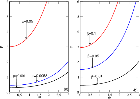
Figure 3: The critical curves for chaotic motions of a modified Rayleigh-Duffing oscillator in a single well potential case in $(\omega,F)$ plane with $\lambda=0.3$, $\delta=-0.08$; $(a):$ effect of pure cubic damping coefficient $\mu$ and $(b):$ effect of pure quadratic damping coefficient $\beta$.

3.2 A three wells potential case

In this subsection, the three wells type (the bounded double hump potential: Fig.2), the system Eq. (9) also has two hyperbolic fixed points and each point process two different types of orbit: a heteroclinic orbit connecting the two saddle points an defined as [Siewe Siewe et al., 2005]:

$$(x_{he},y_{he})=\left(\pm\frac{x_{1}\sqrt{2}\cosh(\frac{\theta t}{2})}{\sqrt{(\Psi+\cosh{\theta t)}}},\quad\mp\frac{\theta x_{1}\sqrt{2}(1-\Psi)\sinh(\frac{\theta t}{2})}{2\sqrt{(\Psi+\cosh{\theta t)^{3}}}}\right)$$ (24)

and a symmetric pair of homoclinic trajectories connected each point to itself given by

$$(x_{ho},y_{ho})=\left(\pm\frac{x_{1}\sqrt{2}\sinh(\frac{\theta t}{2})}{\sqrt{(-\Psi+\cosh{\theta t)}}},\quad\pm\frac{\theta x_{1}\sqrt{2}(1-\Psi)\cosh(\frac{\theta t}{2})}{2\sqrt{(-\Psi+\cosh{\theta t)^{3}}}}\right),$$ (25)

where

$$\theta=x_{1}^{2}\sqrt{2\delta(\rho^{2}-1)}{2};\quad\alpha^{2}=x_{2}^{2}(\rho^{2}+3);\quad\Psi=\frac{5-3\rho^{2}}{3\rho^{2}-1};$$ (26)

$$\rho^{2}=\frac{\lambda+\sqrt{\lambda^{2}-4\delta}}{-\lambda+\sqrt{\lambda^{2}-4\delta}},$$

and

$$x_{1}=\sqrt{\frac{-1}{2\delta}(\lambda+\sqrt{\lambda^{2}-4\delta})},$$

$$x_{2}=\sqrt{\frac{-1}{2\delta}(\lambda-\sqrt{\lambda^{2}-4\delta})}.$$

Let us first consider the case of heteroclinic orbit. After substituting the equations of the heteroclinic orbits $x_{h}$ and $y_{h}$ given in Eq. (24) into Eq. (16), we calculate the Melnikov function and a sufficient condition for the appearance of chaos in sense of Smale is given by

$$F\geq\frac{\theta\sinh(\frac{\pi\omega}{\theta})}{2\pi\omega x_{1}}\left[\frac{2(1+\Psi)\mu}{x_{1}^{2}\theta\chi_{he}}+\frac{2x_{1}^{3}\theta^{2}(13-\Psi)\beta}{105(1-\Psi)}\right],$$ (27)

where

$$\chi_{he}=2+\Psi+\frac{\theta^{2}x_{1}^{2}\Xi_{he}}{160(1+\Psi)^{3}}+\frac{\arcsin\Psi+\frac{\pi}{2}}{\sqrt{1-\Psi^{2}}}\left[1+2\Psi+\frac{\theta^{2}x_{1}^{2}\Delta_{he}}{160(1+\Psi)^{3}}\right],$$

with

$$\Xi_{he}=\frac{402\Psi^{4}+4231\Psi^{3}+5063\Psi^{2}+4448\Psi+976}{3(\Psi-1)}$$

and

$$\Delta_{he}=\frac{2082\Psi^{4}+3696\Psi^{3}+5889\Psi^{2}+405\Psi+135}{3(\Psi-1)}.$$

From each of these relations, the threshold values of the parameters for which the stable and unstable manifolds to the heteroclinic point intersect are obtained and the complicated behavior occurs whenever the above condition is realized. We study the chaotic threshold as a function of only the frequency parameter $\omega$. A typical plot is shown in Fig. 4, in which the critical heteroclinic bifurcation curves are plotted versus the frequency parameter $\omega$. Figs.4 $(a),(b)$ show the critical external forcing amplitude for different values of $\mu$ and $\beta$ respectively. One can see (Fig.4 $(a)$) that when the value of the cubic damping parameter $\mu$ increases, the thresholds of the critical values for heteroclinic bifurcation of the harmonic excitation $F$ increase. The contrary effect is observed with the pure quadratic damping coefficient $\beta$ (Figs.4 $(b)$). We concluded that the parameters $F$ and $\mu$ have the same effect on the critical value for chaotic motions which is the opposit one of parameter $\beta$.

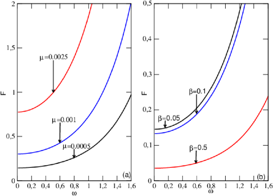
Figure 4: The critical curves for heteroclinic chaos of a modified Rayleigh-Duffing oscillator in a single well potential case in $(\omega,F)$ plane with $\lambda=-0.6$, $\delta=0.05$; $(a):$ effect of pure cubic damping coefficient $\mu$ and $(b):$ effect of pure quadratic damping coefficient $\beta$.

Now, consider the case of homoclinic orbit. Substituting Eq. (25) into Eq. (16), we calculate the Melnikov function. It is known that the intersections of the homoclinic orbits are the necessary conditions for the existence of chaos. The Melnikov function theory measures the distance between the perturbed stable and unstable manifolds in the Poincaré section. If $M^{\pm}(t0)$ has a simple zero, then a homoclinic bifurcation occurs, signifying the possibility of chaotic behavior. This means that only necessary conditions for the appearance of strange attractors are obtained from the Poincaré-Melnikov-Arnold analysis, and therefore one always has the chance of finding the sufficient conditions for the elimination of even transient chaos. Then the necessary condition for which the invariant manifolds intersect is given by

$$F\geq\frac{\theta}{2x_{1}\sin(\frac{2\omega}{\theta})}\left[\frac{x_{1}^{2}\mu\theta\chi_{ho}}{4(1+\Psi)^{2}}+\frac{2\sqrt{2}k_{1}}{15(1+\Psi)^{2}}\right],$$ (28)

where

$$\chi_{ho}=\Psi^{2}+3\Psi-2-\frac{\theta^{2}x_{1}^{2}\Xi_{ho}}{120(1+\Psi)^{2}}+\frac{\arcsin\Psi-\frac{\pi}{2}}{\sqrt{1-\Psi^{2}}}\times$$ (29)

$$\left[\Psi(3\Psi-1)-\frac{\theta^{2}x_{1}^{2}\Delta_{ho}}{120(1+\Psi)^{2}}\right];$$

with

$$\Xi_{ho}=\frac{5\Psi^{5}+42\Psi^{4}+603\Psi^{3}+561\Psi^{2}+566\Psi+112}{\Psi-1};$$

and

$$\Delta_{ho}=\frac{320\Psi^{4}+400\Psi^{3}+765\Psi^{2}+315\Psi+90}{\Psi-1}.$$

These conditions provided a domain of the parameters where the system has transverse homoclinic orbits resulting in possible chaotic behavior. In order to have a visual information, we have plotted in Figs.5 $(a),(b)$ the dependence of the external excitation $F$ on the frequency $\omega$ for different values of $\mu$ and $k_{1}$ respectively. These figures, show that the parameters $\mu$ and $k_{1}$ have the opposit effect on the homoclinic critical value for chaotic motions.

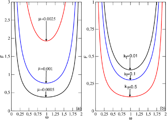
Figure 5: The critical curves for homoclinic chaos of a modified Rayleigh-Duffing oscillator in a triple well potential case in $(\omega,F)$ plane with $\lambda=-0.6$, $\delta=0.05$; $(a):$ effect of pure cubic damping coefficient $\mu$ and $(b):$ effect of unpure quadratic damping coefficient $k_{1}$

4 Numerical simulations and analysis

In order to verify the analytical results obtained in the previous sections, we have numerically integrated the system by using a fourth order Runge-Kutta algorithm to investigate the heteroclinic and the homoclinic chaos in the model. We consider the single well and triple well cases. We checked the effect of the nonlinear damping terms on the motion of the oscillator. In the same vein, we investigated how the basins of attraction are affected as the parameter $\mu,\beta,k_{1}$ and $F$ varied. We see through Figs.6, 7 and 8 that the basin boundaries become fractal or basin of attraction is destroyed. The blue zone stands for the area where the choice of the initial conditions leads to a chaotic motion while the white area is the domain of periodic or quasi-periodic oscillations. This means that the damping parameter $\mu,\beta,k_{1}$ and amplitude of external forced $F$ have contributed to These numerical results obtained confirm exactly the analytical results.

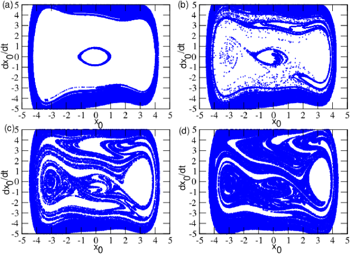
Figure 6: Basin of attraction in heteroclinic chaos of a modified Rayleigh-Duffing oscillator in a triple well potential: $(a)F=0.05,(b)F=0.1,(c)F=0.4$ and $(d)F=0.85$, the others parameters are $\lambda=-0.6,\delta=0.05,k_{1}=0.05,\beta=0.05,\mu=0.0005,\omega=1$.

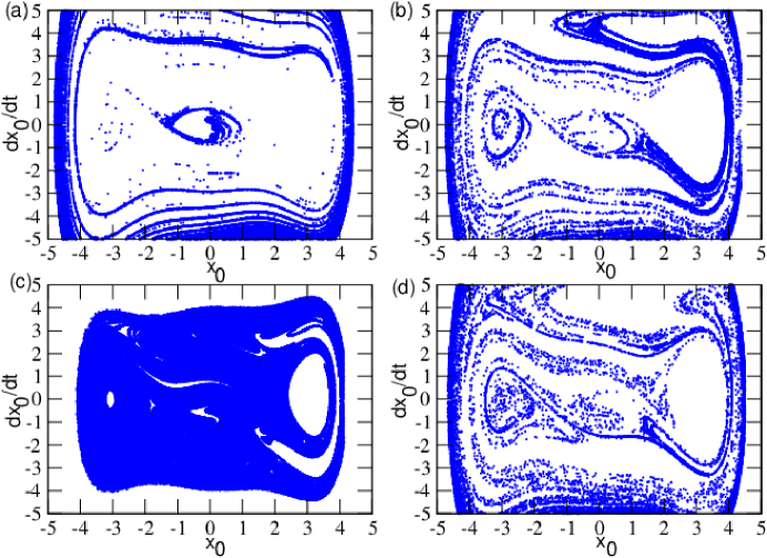
Figure 7: Basin of attraction in homoclinic chaos of a modified Rayleigh-Duffing oscillator in a triple well potential: $(a)F=0.1,(b)F=0.4,(c)F=0.5$ and $(d)F=0.85$, the others parameters are $\lambda=-0.6,\delta=0.05,k_{1}=0.1,\beta=0.05,\mu=0.0005,\omega=1$.

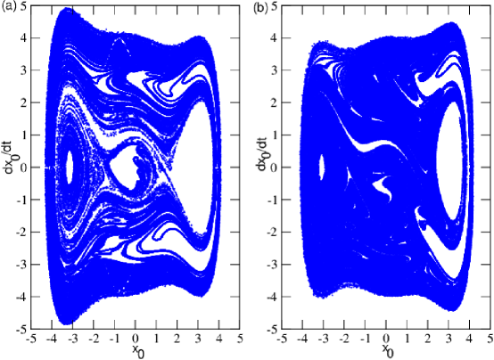
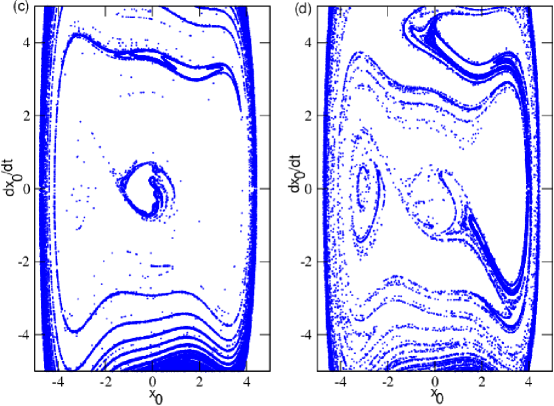
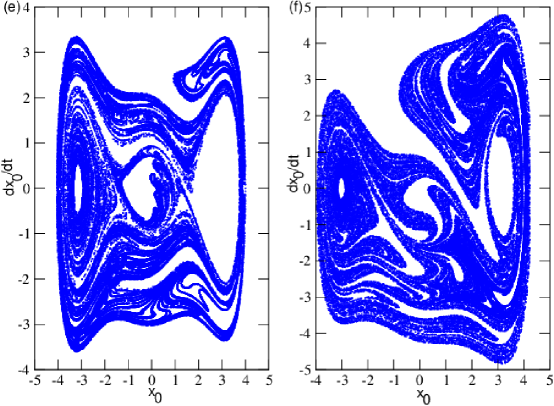
Figure 8: Effects of nonlinear damping parameters on basin of attraction in the triple well potential $(a)$ and $(b)$ effect of $F$, $(c)$ and $(d)$ effects of $k_{1}$ and $(e)$ and $(f)$ effects of $\mu$.

5 Discussion and conclusions

In this paper, the dynamics of a forced nonlinear damped system, the $\phi^{6}$ modified Rayleigh-Duffing oscillator has been studied. The analytical criteria for the appearance of chaos in the sense of Smale have also been derived using Melnikov theory. The effects of nonlinear damping and amplitude of external forced on Melnikov critical values have been investigated. In the single well potential case, we noticed that the nonlinear damping parameters $\mu$ and $\beta$ and the forced amplitude $F$ have the same effects. Melnikov critical value increases with each of these parameters. The parameters $\mu$ and $F$ have the same effects on homoclinic and heteroclinic Melnikov criterion in three well potential case but the quadratic damping $\beta$ and $k_{1}$ have the contrary effects. It should be noted that the pure quadratic damping affected the heteroclinic bifurcation and unpure quadratic damping affected the homoclinic bifurcation. A convenient demonstration of the use and accuracy of the method, is obtained from the basin of attraction. By means of the basin of attraction, we have shown that for certain regions of parameter space, the deterministic system driven harmonically experience behaviors that may be chaotic or non-chaotic.

Finally, the above assessment reveals that roll damping is a very critical parameter in motion characteristics of a ship. Therefore estimation of roll damping may lead to accurate prediction of chaotic ship rolling motions. In principle, it may be explained as the influence between nonlinear damping and excitation force.

Acknowlegments

The authors thank IMSP for financial support. We also thank Professor Paul Woafo, Professor Roméo Nana Nbendjo an Doctor hervé Enjieu Kadji for their suggestions and collaboration.

References

- [1] Bikdash, M., Balachandran, B. & Nayfeh, A. [1994] “Melnikov analysis for a ship with a general roll damping model,” Nonlin. Dyn 6, 101–124.
- [2] Enjieu Kadji, H.G. & Nana Nbendjo, B.R. [2012] “ Passive aerodynamics control of plasma instabilities,”Commun Nonlinear Sci Numer Simulat 17, 1779–1794.
- [3] Falzarano, J. M. [1990] Predicting complicated dynamics leading to vessel capsizing, PhD Dissertation, Departement of Naval Architecture, The University of Michigan.
- [4] Falzarano, J. M., Shaw, S. W. & Troesch, A. W. [1992] “Application of global methods for analyzing dynamical systems to ship rolling motion and capsizing,” Int.J. Bifurcation and Chaos 2, 101-115.
- [5] Francescutto, A. & Contento, G. [1999] “Bifurcations in ship rolling: experimental results and parameter identification technique,” Ocean Engineering 26,1095–1123.
- [6] Hayashi, C. [1964] Nonlinear Oscillations in Physical Systems ( McGraw-Hill, New York).
- [7] Holappa, K. W. & Falzarano, J. M. [1999] “Application of extended state space to nonlinear ship rolling,” Ocean Engineering 26, 227–240.
- [8] Litak, G., Borowiec, M., Friswell, M. I. & Szabelski, K. [2008] “Chaotic vibration of a quarter-car model excited by the road surface profile,” Communications in Nonlinear Science and Numerical Simulation 13, 1373–1383.
- [9] Litak, G., Borowiec, M., Syta, A. & Szabelski, K. [2009] “Transition to Chaos in the Self-Excited System with a Cubic Double Well Potential and Parametric Forcing,” Chaos, Solitons and fractals 40, 2414–2429.
- [10] Miwadinou, C.H., Monwanou, A. V. & Chabi Orou, J. B. [2014] “Active Control of the Parametric Resonance in the Modified Rayleigh-Duffing Oscillator,” African Review of Physics 9, 227–235.
- [11] Miwadinou, C.H., Monwanou, A. V. & Chabi Orou, J. B. [2015] “Effect of Nonlinear Dissipation on the Basin Boundaries of a Driven Two-Well Modified Rayleigh-Duffing Oscillator,” Int. J. Bifurcation and Chaos 25, No. 2 (2015) 1550024 (14 pages).
- [12] Nana Nbendjo, B.R., Yamapi, R. [2007] “Active control of extended Van der Pol equation,” Communications in Nonlinear Science and Numerical Simulation 12, 1550–1559.
- [13] Nayfeh, A. H., & Mook, D. T. [1979] Nonlinear Oscillations ( Wiley, New York).
- [14] Rand, R. H., Ramani, D. V., Keith, W. L. & Cipolla, K. M. [2000] “The quadratically damped Mathieu equation and its application to submarine dynamics,”Control of Vibration and Noise, New Millennium 61, 39–50.
- [15] Ravindra, B. & Mallik, A. K. [1994a] “Stability analysis of a non-linearly damped Duffing oscillator,” J. Sound Vib 171, 708–716.
- [16] Ravindra, B. & Mallik, A. K. [1994b] “ Role of nonlinear dissipation in soft Duffing oscillators,” Phys. Rev.E 49, 4950–4954.
- [17] Sanjuán, M. A. F. [1999] “The effect of nonlinear damping on the universal escape oscillator,” Int. J. Bifurcation and Chaos 9, 735–744.
- [18] Scolan, Y. M. [1999] “Application of the Melnikov method to nonlinear ship rolling in waves,” Comptes Rendus de l’Academie des Sciences Series IIB Mechanics Astronomy 327, 1–6.
- [19] Siewe Siewe, M., Moukam Kakmeni, F. M., Tchawoua, C. [2004] “Resonant oscillation and homoclinic bifurcation in a -Van der Pol oscillator,”Chaos, Solitons and Fractals 21, 841–853.
- [20] Siewe Siewe, M., Moukam Kakmeni, F. M., Tchawoua, C. & Woafo, P. [2005] “Bifurcations and chaos in the triple-well -Van der Pol oscillator driven by external and parametric excitations,”Physica A 357, 383–396.
- [21] Siewe Siewe, M., Moukam Kakmeni, F. M., Tchawoua, C. & Woafo, P. [2006] “Nonlinear Response and Suppression of Chaos by Weak Harmonic Perturbation inside a Triple Well -Rayleigh Oscillator Combined to Parametric Excitations,”Journal of Computational and Nonlinear Dynamics 1, 196–204.
- [22] Siewe Siewe, M., Cao, H. & Sanjuán, M. A. F. [2009] “On the occurrence of chaos in a parametrically driven extended Rayleigh oscillator with three-well potential,” Chaos, Solitons and fractals 41, 772–782.
- [23] Soliman, M. S. & Thompson, J. M. T. [1992] “The effect of damping on the steady state and basin bifurcation patterns of a nonlinear mechanical oscillator,”Int. J. Bifurcation and Chaos 2, 81–91.
- [24] Spyrou, K.J., Cotton, B., Gurd, B., [2002] “ Analytical expressions of capsize boundary for a ship with roll bias in beam waves,” Journal of Ship Research 46, 167–174.
- [25] Taylan, M. [2000] “The effect of nonlinear damping and restoring in ship rolling,” Ocean Engineering 27, 921–932
- [26] Tchoukuegno, R. & Woafo, P. [2002] “ Dynamics and active control of motion of a particle in a potential with a parametric forcing,” Physica D 167, 86–100.
- [27] Tchoukuegno, R., Nana Nbendjo, B. R. & Woafo, P. [2003] “ Linear feedback and parametric controls of vibration and chaotic escape in a potential,” Int J Non-Linear Mech 38, 531–541.
- [28] Wan, W. & Leigh, M. [2008] “Application of the extended Melnikov’s method for single-degree-of-freedom vessel roll motion,”Ocean Engineering 35, 1739–1746.
- [29] Yamapi, R., Chabi Orou, J. B. & Woafo, P. [2003] “Harmonic oscillations, stability and chaos control in a nonlinear electromechanical system,” J. Sound Vibr 259, 1253–1264.
- [30] Yamapi, R., Nana Nbendjo, B.R. & Enjieu Kadji, H.G. [2007] “ Dynamics and active control of motion of a driven multi-limit-cycle Van der pol oscillator,” Int. J. Bifurcation and Chaos 17,1343–1354.