Tunable unconventional Kondo effect on topological insulator surfaces

Abstract

We study Kondo physics of a spin-$\frac{1}{2}$ impurity in electronic matter with strong spin-orbit interaction, which can be realized by depositing magnetic adatoms on the surface of a three-dimensional topological insulator. We show that magnetic properties of topological surface states and the very existence of Kondo screening strongly depend on details of the bulk material, and specifics of surface preparation encoded in time-reversal preserving boundary conditions for electronic wavefunctions. When this tunable Kondo effect occurs, the impurity spin is screened by purely orbital motion of surface electrons. This mechanism gives rise to a transverse magnetic response of the surface metal, and spin textures that can be used to experimentally probe signatures of a Kondo resonance. Our predictions are particularly relevant for STM measurements in ${\rm PbTe}$-class crystalline topological insulators, but we also discuss implications for other classes of topological materials.

I Introduction

Recent explosion of interest in topological insulators (TIs) Zhang et al. (2009); Hasan and Kane (2010); Qi and Zhang (2011) is due in large part to the fact that they support metallic states on their surfaces. The existence of these states (and hence the metallicity) results from the non-trivial topological nature of the Bloch wavefunctions in the conduction and valence bands of the bulk material, and is a robust feature. In contrast, the quantum numbers associated with those surface states are not determined by topology alone. Therefore they may vary from material to material, and depend on the surface preparation. Understanding physical consequences of this non-universal behavior is one of the foci of our paper.

A typical cartoon picture of surface states in a TI consists of spin-momentum-locked energy branches of a massless Dirac spectrum. This description cannot be universally accurate. A crystal boundary breaks the inversion symmetry and gives rise to strong, rapidly varying in space, electric fields that define an effective surface potential for the electrons. Interplay between these field gradients and the bulk inter-atomic spin-orbit interaction (SOI), responsible for the non-trivial topological aspects of these materials, renders this potential momentum and spin dependent. As we show below, this ensures that measurable properties of the surface states cannot be determined by topological arguments alone. Details associated with a crystal surface can be accounted for via effective boundary conditions (BCs) for the electron wavefunctions Volkov and Pinsker (1981); Potapenko and Satanin (1984), and are completely excluded from the topological arguments involving only the bulk band structure. In this context, Ref. Isaev et al., 2011 argued that appropriate BCs are essential for a sensible formulation of a bulk-boundary correspondence in TIs. Moreover, Ref. Zhang et al., 2012 pointed out a dependence of the spin texture of surface Dirac cones on the crystallographic orientation of the surface, even for simple BCs.

In this paper we show that the spin behavior of surface states in three-dimensional (3D) TIs is highly sensitive to both the bulk band structure and surface properties. We consider semiconductors with different crystal symmetry: cubic lead chalcogenides (${\rm PbTe}$ or ${\rm PbSe}$) and tetragonal ${\rm Bi_{2}Se_{3}}$-like TIs, and demonstrate that magnetic probes (such as an external field or quantum impurities) can be used to efficiently differentiate between these two classes. Crucially, the sensitivity of TI surface states to the surface manipulation allows one to use TIs as a controllable environment for studying spin-dependent correlated phenomena in the presence of strong SOI.

While some of the unusual magnetic phenomena that we argue for can be probed by measuring the response to a uniform magnetic field, in this paper we focus on the physics of a spin-$\frac{1}{2}$ impurity deposited on the surface of a 3D TI. Kondo screening, whereby the impurity spin at low temperatures forms a singlet state with the Fermi sea, is one of the earliest and lucid examples of correlated many-body physics Wilson (1975) that remains relevant in contexts ranging from heavy fermion systems Hewson (1997); Cox and Zawadowski (1999) to nanoscience Kikoin et al. (2011). Advances in scanning tunneling microscopy (STM) allowed observation of this phenomenon on the atomic scale Madhavan et al. (1998); Li et al. (1998); Prüser et al. (2011), and granted access to manipulation of individual Kondo resonances Tsukahara et al. (2011). Testing surface states of TIs via STM Roushan et al. (2009) complements spin-polarized angle-resolved photoemission (ARPES) measurements Hsieh et al. (2009); Herdt et al. (2013), and gives a direct probe of the Kondo effect.

In its simplest form, Kondo screening involves only spin degrees of freedom of the conduction electrons. Hence it is sensitive to the spin-$SU(2)$ symmetry breaking, provided in our case by the SOI. Previous works have shown that the Kondo effect survives in the presence of spin-orbit scattering Bergmann (1986); Wei et al. (1989); Meir and Wingreen (1994), and weak (compared to the bandwidth) Rashba or Dresselhaus band SOI Malecki (2007); Yanagisawa (2012); Mastrogiuseppe et al. (2014); Žitko and Bonča (2011); Feng et al. (2010); Hu et al. (2013). In some cases, the latter can actually enhance the Kondo resonance Isaev et al. (2012); Zarea et al. (2012). The strong SOI regime is even more intriguing. Indeed, the SOI can be viewed as a momentum-space magnetic “field” that aligns electron spins along a particular direction (e.g. perpendicular to its momentum). When this field is large enough the spin degree of freedom of conduction electrons is effectively lost and cannot participate in the spin-flip scattering leading to the Kondo effect. Nevertheless there is substantial theoretical evidence Zitko (2010); Tran and Kim (2010); Feng et al. (2010); Mitchell et al. (2013); Orignac and Burdin (2013); Xin and Yeh (2013) indicating that a magnetic impurity on a TI surface is screened by the surface metal. Remarkably the physical nature of this effect and spatial structure of the screening states have never been elucidated in the context of TIs. Understanding this phenomenon is also important from an experimental perspective because magnetic probes (e.g. impurities or magnetic field) coupled to surface electrons can be used to differentiate trivial and topologically non-trivial matter, providing an alternative to ARPES-based techniques.

We demonstrate that the strong SOI leads to an unconventional Kondo effect with an impurity spin screened by purely orbital motion of surface electrons. Specifically, we consider a simple band model of a 3D TI, and derive an effective Kondo Hamiltonian that governs the dynamics of the impurity spin at the TI boundary (that does not break time-reversal symmetry), taking into account the full 3D spatial dependence of surface-state wavefunctions. Because of the SOI this Kondo exchange has an $XXZ$ structure and, in general, is strongly anisotropic. At low energies, the impurity spin forms a singlet state with the total electron angular momentum, and the system exhibits an emergent $SU(2)$ symmetry, which is responsible for the Kondo resonance. The SOI also gives rise to a transverse magnetic response when an external magnetic field applied normal to the surface results in an in-plane electron spin polarization, which may lead to interesting magneto-electric phenomena under driving fields. This response is significantly stronger than an analogous effect on metallic surfaces with Rashba SOI Lounis et al. (2012); Chirla et al. (2013).

In Sec. II, we describe our minimal model of a 3D TI and calculate its surface spectrum. Here we consider a continuum version of a lattice model studied in Ref. Isaev et al., 2011. Emphasis is put on the physical meaning of the quantum numbers involved in the effective description of electronic states. In Sec. III we explain how both surface and bulk states play a role in determining the specific mathematical form of the relevant operators involved in the effective coupling between surface electrons of the TI and the magnetic impurity. Here, we contrast ${\rm Bi_{2}Se_{3}}$ and ${\rm PbTe}$-class materials. Section IV establishes the effective $XXZ$ Kondo Hamiltonian that governs coupling of these surface states to magnetic impurities, and explains why this is a single-channel Kondo Hamiltonian despite its apparent two-channel form. In our approach we control the surface properties through BCs for electronic wavefunctions Isaev et al. (2011) and show that surface manipulation provides an effective way of tuning parameters in the effective low-energy Kondo model and can be used to completely suppress the spin-flip terms and destabilize the Kondo effect. We study the physical properties of the effective model and its unconventional Kondo physics in Sec. V. In particular, we investigate the transverse magnetic response to an external magnetic field and point to the resulting transverse spin textures as a distinctive characteristic of the Kondo screening cloud in strong SOI materials. We also show how one can tune the Kondo effect and the characteristic temperature $T_{K}$ via surface manipulation. Our results can be directly verified in STM measurements in crystalline TIs like the lead-tin solid alloys ${\rm Pb_{1-x}Sn_{x}Te}$, but the above unconventional Kondo physics can also be observed in well-studied ${\rm Bi_{2}Se_{3}}$ and ${\rm BiSb}$. Finally, Sec. VI provides a summary and an outlook with questions that still remain open. Two appendices with technical derivations complete the paper: Appendix A addresses the very important problem of self-adjoint extensions of unbounded Hermitian operators, of key relevance to the analysis of bound surface states. Appendix B exploits the axial symmetry of the problem to construct surface states with well-defined total angular momentum.

II Simple continuum model for topological insulators

II.1 Model Hamiltonian

To describe electronic states in a TI we use Dimmock’s model Carter and Bate (1971); Kang and Wise (1997), defined by the modified Dirac Hamiltonian

$$H_{\rm D}=v({\bm{\alpha}}\cdot{\bm{p}})+\beta\biggl{(}\Delta+\frac{{\bm{p}}^{2}}{2m^{*}}\biggr{)}.$$ (1)

This effective Hamiltonian involves two spinful bands (conduction and valence) of opposite parity separated by an energy gap $2\Delta$ and is written in terms of the $4\times 4$ Dirac matrices

$${\bm{\alpha}}=(\sigma^{x}\otimes{\bm{\sigma}})=\begin{pmatrix}0&{\bm{\sigma}}\\ {\bm{\sigma}}&0\end{pmatrix},\quad\beta=(\sigma^{z}\otimes{\bm{1}})=\begin{pmatrix}{\bm{1}}&0\\ 0&-{\bm{1}}\end{pmatrix},$$

with ${\bm{\sigma}}=(\sigma^{x},\sigma^{y},\sigma^{z})$ denoting the usual Pauli matrices, and ${\bm{1}}$ – the unit $2\times 2$ matrix. In Eq. (1) the effective mass $m^{*}$ accounts for contributions from remote bands, and the velocity scale $v$ is proportional to the momentum matrix element between conduction and valence Bloch states. In the following we shall adopt units with $\hbar=1$.

The Dimmock Hamiltonian (1) provides a standard description of electronic spectra in lead chalcogenides near one of the 8 equivalent $L$-points in the Brillouin zone. Note that despite the presence of SOI Eq. (1), is written in the basis of direct-product states Kang and Wise (1997) $|L_{6}^{\pm}\rangle\otimes|\sigma\rangle$, where $L_{6}^{\pm}$ denote spinor one-dimensional representations of $D_{3d}$ corresponding to the conduction ($L_{6}^{-}$) and valence ($L_{6}^{+}$) bands, superscripts $\pm$ indicate spatial parity of the state, and $\sigma={\uparrow}$, ${\downarrow}$ is the electron spin quantum number. Eigenstates of $H_{\rm D}$ are 4-component envelope functions

$$\psi({\bm{x}})=\begin{pmatrix}\psi_{c,1}({\bm{x}})\\ \psi_{c,2}({\bm{x}})\\ \psi_{v,1}({\bm{x}})\\ \psi_{v,2}({\bm{x}})\end{pmatrix}\!\!,\,\,\psi^{\dagger}({\bm{x}})=\bigl{(}\psi_{c,1}^{*}\,\psi_{c,2}^{*}\,\psi_{v,1}^{*}\,\psi_{v,2}^{*}\bigr{)},$$

which define the full electron wavefunction in the crystal: $\langle{\bm{x}}|\Psi\rangle=\sum_{i=1,2}[\psi_{c,i}({\bm{x}})\langle{\bm{x}}|u_{c,i}({\bm{k}}_{0})\rangle+\psi_{v,i}({\bm{x}})\langle{\bm{x}}|u_{v,i}({\bm{k}}_{0})\rangle]{\rm e}^{{\rm i}{\bm{k}}_{0}{\bm{x}}}$ where $\langle{\bm{x}}|u_{(c,v),i}({\bm{k}}_{0})\rangle{\rm e}^{{\rm i}{\bm{k}}_{0}{\bm{x}}}$ are Bloch states corresponding to band extrema at the point ${\bm{k}}_{0}$ in the Brillouin zone (${\bm{k}}\cdot{\bm{p}}$ method). The state $|\Psi\rangle$ does not need to have a definite spin quantum number due to the SOI usually present in TIs. In general, the indices $i=1,2$ describe pseudospin states whose relation to the true spin will depend on the material. For instance, in ${\rm PbSe}$-like systems the gap at the $L$-point is formed by non-degenerate representations of the single group $D_{3d}$. The SOI does not affect these states besides shifting their energy, so the pseudospin states $i=1,2$ can be identified with the eigenstates of $\sigma^{z}$ [i.e. $|\sigma\rangle=|{\uparrow}\rangle$ or $|{\downarrow}\rangle$] Kang and Wise (1997). The (periodic part of the) Bloch basis functions can be taken as direct products of orbital and spin parts $|u_{c,i}({\bm{k}}_{0})\rangle=|u_{c}({\bm{k}}_{0})\rangle\otimes|\sigma\rangle$.

The Hamiltonian (1) has a number of conserved “tensor” spin operators Bagrov and Gitman (1990). For us the important one is

$${\bm{T}}=\beta[{\bm{\Sigma}}\times{\bm{p}}]={\rm diag}\bigl{\{}[{\bm{\sigma}}\times{\bm{p}}],\,-[{\bm{\sigma}}\times{\bm{p}}]\bigr{\}},$$ (2)

with ${\bm{\Sigma}}=(1\otimes{\bm{\sigma}})$. One can easily check that $[H_{\rm D},{\bm{T}}]=0$. Here we will only need $T^{z}={\rm i}\beta\alpha^{z}({\bm{\alpha}}^{\perp}\cdot{{\bm{p}}_{\perp}})$, where “$\perp$” denotes $xy$ vector components. The Dimmock Hamiltonian (1) can be rewritten as

$$H_{\rm D}=v\bigl{(}\alpha^{z}p_{z}+{\rm i}\beta\alpha^{z}T^{z}\bigr{)}+\beta\biggl{(}\Delta+\frac{{\bm{p}}^{2}}{2m^{*}}\biggr{)}.$$ (3)

Note, that $T^{z}$ is a block-diagonal matrix whose elements are proportional to a “Rashba” SOI term $[{\bm{\sigma}}\times{{\bm{p}}_{\perp}}]_{z}$.

Effective mass models similar to (1) emerge in many narrow-gap semiconductors with strong SOI Bir and Pikus (1974), such as ${\rm Bi_{2}Se_{3}}$. The relevant point in the Brillouin zone and the interpretation of the quantum numbers may differ depending on the material. For example, in ${\rm Bi_{2}Se_{3}}$ (symmetry $D_{3d}$ at the $\Gamma$-point) the SOI is essential in determining gap-forming states Zhang et al. (2009), hence the basis states are no longer direct products. Even though there are still four states in the vicinity of the gap and the effective mass description is given by Eq. (1), the identification of the pseudospin with real spin (as for ${\rm PbSe}$) is no longer possible. These considerations are important for deriving an effective mass interaction Hamiltonian between the surface electrons and external probes such as magnetic field or magnetic impurities. Naturally, this interaction will depend on details of the bulk band structure of a material. Below we are going to illustrate this point by comparing the coupling of surface states and localized magnetic moments in lead and bismuth selenide compounds.

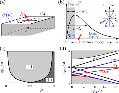
Figure 1: Panel (a) Geometry of the problem. The TI occupies half-space $z\geqslant 0$. The unit vector ${\bm{n}}$ is an outer normal to the surface. The red arrow represents the impurity spin. (b) Schematic $z$-dependence of the surface state wavefunction (6), characterized by two length scales: small $1/\lambda\sim 1/m^{*}v$ (shaded region) and large $1/q\sim v/\Delta$. The Dirac model (7) is valid at distances $\geqslant 1/q$. The impurity is located under the surface where the Dirac theory is applicable. The inset shows the dispersion of surface modes. (c) Stability diagram of surface states (10). Thick lines correspond to critical momenta $p_{\perp}^{cr}=\pm(\Delta/v)\,{\rm ctg}\,\vartheta$. In the white region no surface states can exist. In the (light) dark gray area, there are surface modes with (only one, $\tau=-1$) both helicites. (d) Dispersion relation (10) for several values of $\vartheta$. The upper (lower) branches (relative to the point $p_{\perp}=0$) correspond to $\tau=\mp 1$. The Fermi energy is $\varepsilon_{F}=0$.

II.2 Quasiparticle states in a half-space

We are particularly interested in the localized surface states that form as a result of breaking translational invariance. Consider a TI bounded by the surface $z=0$ whose bulk states are described by $H_{\rm D}$, see Fig. 1(a). It follows that ${{\bm{p}}_{\perp}}$ is conserved and, together with $T^{z}$, can be used to classify quasiparticles states. An eigenfunction $\psi_{{{\bm{p}}_{\perp}}\tau}$ of $T^{z}$, $T^{z}\psi_{{{\bm{p}}_{\perp}}\tau}=\tau p_{\perp}\psi_{{{\bm{p}}_{\perp}}\tau}$, has the form

$$\psi_{{{\bm{p}}_{\perp}}\tau}({\bm{x}})=\begin{pmatrix}a(z)U_{{{\bm{p}}_{\perp}}\tau}\\ b(z)U_{{{\bm{p}}_{\perp}},-\tau}\end{pmatrix}{\rm e}^{{\rm i}{{\bm{p}}_{\perp}}\cdot{\bm{x}}_{\perp}}.$$

with

$$U_{{{\bm{p}}_{\perp}}\tau}=\frac{1}{\sqrt{2}}\begin{pmatrix}1\\ -{\rm i}\tau{\rm e}^{{\rm i}\phi_{{\bm{p}}_{\perp}}}\end{pmatrix},$$ (4)

where $p_{\perp}=|{{\bm{p}}_{\perp}}|$ and ${\rm e}^{{\rm i}\phi_{{\bm{p}}_{\perp}}}=(p_{x}+{\rm i}p_{y})/p_{\perp}$. The amplitudes $a(z)$ and $b(z)$ are determined by solving the remaining $2\times 2$ boundary value problem. In Eq. (3) one can now replace $T^{z}$ with $\tau p_{\perp}$, hence reducing the number of independent Dirac matrices to two: $\beta$ and $\alpha^{z}$. Their action on the $z$-dependent spinor part of $\psi_{{{\bm{p}}_{\perp}}\tau}({\bm{x}})$ is equivalent to the action of $\sigma^{z}$ and $\sigma^{x}$ on a two-component wavefunction $(a^{*}\,b^{*})^{\dagger}$

$$\alpha^{z}\begin{pmatrix}a(z)U_{{{\bm{p}}_{\perp}}\tau}\\ b(z)U_{{{\bm{p}}_{\perp}},-\tau}\end{pmatrix}=\begin{pmatrix}b(z)U_{{{\bm{p}}_{\perp}}\tau}\\ a(z)U_{{{\bm{p}}_{\perp}},-\tau}\end{pmatrix}\to \sigma^{x}\begin{pmatrix}a(z)\\ b(z)\end{pmatrix},$$

$$\beta\begin{pmatrix}a(z)U_{{{\bm{p}}_{\perp}}\tau}\\ b(z)U_{{{\bm{p}}_{\perp}},-\tau}\end{pmatrix}=\begin{pmatrix}a(z)U_{{{\bm{p}}_{\perp}}\tau}\\ -b(z)U_{{{\bm{p}}_{\perp}},-\tau}\end{pmatrix}\to \sigma^{z}\begin{pmatrix}a(z)\\ b(z)\end{pmatrix}.$$

which allows us to replace the Hamiltonian (3) with a $2\times 2$ operator

$$H^{(2\times 2)}_{\rm D}=v\bigl{(}\sigma^{x}p_{z}-\sigma^{y}\tau p_{\perp}\bigr{)}+\sigma^{z}\biggl{(}\Delta+\frac{{\bm{p}}^{2}}{2m^{*}}\biggr{)}$$ (5)

acting on two-component $z$-dependent wavefunctions. This reduction of dimension (from 4 to 2) is a direct consequence of conservation of $T^{z}$.

An important insight can be obtained by studying the simplest case of a hard boundary at $z=0$ where the wavefunction vanishes, $\psi|_{z=0}=0$. Surface states with energy $\epsilon_{{{\bm{p}}_{\perp}}\tau}=\tau vp_{\perp}$ exist for an inverted band structure when $-m^{*}v^{2}/2<\Delta<0$ Kisin and Petrosyan (1987). The surface-state (unnormalized) wavefunction is a coherent superposition of the conduction and valence bands

$$\psi_{{{\bm{p}}_{\perp}}\tau}({\bm{x}})\sim\begin{pmatrix}U_{{{\bm{p}}_{\perp}}\tau}\\ -{\rm i}U_{{{\bm{p}}_{\perp}},-\tau}\end{pmatrix}\bigl{(}{\rm e}^{-qz}-{\rm e}^{-\lambda z}\bigr{)}{\rm e}^{{\rm i}{{\bm{p}}_{\perp}}\cdot{\bm{x}}_{\perp}},$$ (6)

and is characterized by two momentum-dependent inverse length scales: $\begin{pmatrix}q\\ \lambda\end{pmatrix}=m^{*}v\mp\sqrt{m^{*}(m^{*}v^{2}+2\Delta)+{{\bm{p}}_{\perp}}^{2}}$. This surface state is stable only when $q>0$, i.e. for $p_{\perp}\leqslant\sqrt{2m^{*}|\Delta|}$ and merges into the scattering continuum for larger $p_{\perp}$. For more complicated BCs, the problem of determining the surface spectrum from microscopic considerations is rather cumbersome (see Ref. Isaev et al., 2011 and Appendix A for details).

It is possible to simplify matters by considering the limit when $m^{*}v\gg|\Delta|/v,\,p_{\perp}$. In this case $vq\approx|\Delta|$ and $\lambda\approx 2m^{*}v\gg q$. These lengths are illustrated in Fig. 1(b). One can build a theory Joe et al. (2007) valid on the scale $\sim 1/q$ by neglecting $1/\lambda$. This small-$p_{\perp}$ perturbative approach is similar to that used in hydrodynamics of weakly viscous fluids Landau and Lifshitz (1963). In the bulk we can simply omit the ${\bm{p}}^{2}/2m^{*}$ term in Eq. (1), so the Hamiltonian takes the Dirac form:

$$H_{0}=v({\bm{\alpha}}\cdot{\bm{p}})+\beta\Delta.$$ (7)

Near the surface (at distances $\sim 1/\lambda$) the situation is more complicated because the term ${\bm{p}}^{2}/2m^{*}\sim\lambda$ and cannot be neglected. Within this layer [shown in gray in Fig. 1(b)] the electronic wavefunction varies rapidly in accordance with the BCs supplementing the Dimmock Hamiltonian (1). However, this complexity can be absorbed into the BC for the Dirac Hamiltonian (7). This BC has to be consistent with the particle conservation, time-reversal and inversion (parity) symmetries, and can be written as Volkov and Pinsker (1981); Potapenko and Satanin (1984); Isaev et al. (2011) $B\psi|_{z=0}=0$ with

$$B=1+\beta\sin\vartheta+{\rm i}\beta({\bm{\alpha}}\cdot{\bm{n}})\cos\vartheta,$$ (8)

and ${\bm{n}}$ – the outer normal to the surface. The boundary operator $B$ includes one free parameter $\vartheta$ which accounts for microscopic properties of a realistic TI surface, and the behavior of the electronic wavefunction at the length scale $\sim 1/m^{*}v$. An exact connection between $\vartheta$ and the boundary conditions of the original fully microscopic Hamiltonian is not unique in the effective long wavelength Dirac model. However, we show in Appendix A that to be self-adjoint in a half-space, the Hamiltonian (7) must have a single-parameter family of BCs. Consequently, variation of the parameter $\vartheta$ allows us to consider entire sets of possible surface properties realized in experiments. Physically, $\vartheta$ controls the amount of particle-hole (p-h) asymmetry at the surface: The p-h symmetric case is recovered only when $\vartheta=0$ or $\pi$. The Dirac model (7) is clearly less complete than the Dimmock theory (1), but it is much easier to work with.

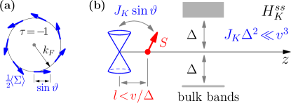
Figure 2: Panel (a) Helical structure of the surface state (10). Blue arrows indicate the expectation value of the electron spin $\frac{1}{2}{\bm{\Sigma}}$ which points perpendicular to the momentum and has a magnitude $\sim\sin\vartheta$. For $\vartheta=\pi$, surface states carry no spin. (b) Schematic illustration of the Kondo interaction $H_{K}$ in Eq. (12). At weak coupling one can ignore bulk-surface mixing induced by the impurity and assume that $H_{K}\approx H_{K}^{ss}$. The impurity only couples to surface states (blue Dirac cone).

From now on we will focus on the problem defined by Eqs. (7) and (8). Since $\vartheta$ can be chosen arbitrarily, we confine our analysis to the case $\Delta>0$ (no band inversion) and $\vartheta\in[0,\pi]$. Results for $\vartheta>\pi$ can be obtained using charge conjugation $\psi\to\alpha^{y}\psi^{*}$. The energy and wavefunction of surface states are given by

$$\epsilon_{{{\bm{p}}_{\perp}}\tau}=\tau vp_{\perp}\cos\vartheta-\Delta\sin\vartheta,$$ (9)

and

$$\psi_{{{\bm{p}}_{\perp}}\tau}({\bm{x}})={\cal N}\begin{pmatrix}(1-\sin\vartheta)U_{{{\bm{p}}_{\perp}}\tau}\\ -{\rm i}\cos\vartheta U_{{{\bm{p}}_{\perp}},-\tau}\end{pmatrix}{\rm e}^{({\rm i}{{\bm{p}}_{\perp}}\cdot{\bm{x}}_{\perp}-q_{{{\bm{p}}_{\perp}}\tau}z)}.$$ (10)

Here ${\cal N}=\sqrt{q_{{{\bm{p}}_{\perp}}\tau}/A(1-\sin\vartheta)}$ and

$$q_{{{\bm{p}}_{\perp}}\tau}=-\tau p_{\perp}\sin\vartheta-(\Delta/v)\cos\vartheta$$ (11)

is the localization wavevector and $A$ – the area of the TI surface [$xy$-plane, see Fig. 1(a)]. The stability region of the state (10) is determined by the condition $q_{{{\bm{p}}_{\perp}}\tau}\geqslant 0$. For $\vartheta>\pi/2$ the $\tau=-1$ state exists for any value of $p_{\perp}$, while the state with $\tau=+1$ is stable only for $vp_{\perp}<-\Delta\,{\rm ctg}\,\vartheta$. For $\vartheta<\pi/2$ the $\tau=+1$ mode is always unstable and the one with $\tau=-1$ exists for $vp_{\perp}>\Delta\,{\rm ctg}\,\vartheta$. These regions are shown in Fig. 1(c). The surface state enters the single-particle continuum at $p_{\perp}=p_{\perp}^{cr}=\pm(\Delta/v)\,{\rm ctg}\,\vartheta$. The function $\epsilon_{{{\bm{p}}_{\perp}}\tau}$ is presented in Fig. 1(d) for several values of $\vartheta$.

Surface states (10) are characterized by a helical spin distribution, shown in Fig. 2(a), that depends on the BC, as one can see by computing an expectation value of the spin $\frac{1}{2}{\bm{\Sigma}}$. This average is $\bigl{\langle}\frac{1}{2}{\bm{\Sigma}}\bigr{\rangle}=\frac{1}{2}{\cal N}^{2}U^{\dagger}_{{{\bm{p}}_{\perp}}\tau}\bigl{[}(1-\sin\vartheta)^{2}\,{\bm{\sigma}}+\cos^{2}\vartheta\,\,\sigma^{z}{\bm{\sigma}}\sigma^{z}\bigr{]}U_{{{\bm{p}}_{\perp}}\tau}=-q_{{p_{\perp}}\tau}\tau\sin\vartheta\,\,(\sin\phi_{{\bm{p}}_{\perp}}{\bm{e}}_{x}-\cos\phi_{{\bm{p}}_{\perp}}{\bm{e}}_{y})\sim\sin\vartheta$, hence at a p-h symmetric point $\vartheta=\pi$, surface states (10) [and (6)] carry no spin. This situation is quite different from the usual case of boundary-independent surface states Hasan and Kane (2010); Qi and Zhang (2011).

The single-particle scattering continua are defined by $\epsilon_{{{\bm{p}}_{\perp}}p_{z}}=\pm\sqrt{v^{2}(p_{z}^{2}+{{\bm{p}}_{\perp}}^{2})+\Delta^{2}}$ with $p_{z}\geqslant 0$. Note that $\epsilon_{{{\bm{p}}_{\perp}}p_{z}}$ is doubly degenerate w.r.t. $\tau$. The corresponding (unnormalized) wavefunction is

$$\psi_{{{\bm{p}}_{\perp}}p_{z}\tau}({\bm{x}})\sim\!\begin{pmatrix}(\Delta+\epsilon_{{{\bm{p}}_{\perp}}p_{z}})\sin\kappa\,\,U_{{{\bm{p}}_{\perp}}\tau}\\ -{\rm i}v\bigl{[}p_{z}\cos\kappa+\tau p_{\perp}\sin\kappa\bigr{]}U_{{{\bm{p}}_{\perp}},-\tau}\end{pmatrix}{\rm e}^{{\rm i}{{\bm{p}}_{\perp}}\cdot{\bm{x}}_{\perp}},$$

where $\kappa=p_{z}z+\zeta$ and

$${\rm tg}\,\zeta=\frac{vp_{z}\cos\vartheta}{(1+\sin\vartheta)(\Delta+\epsilon_{{{\bm{p}}_{\perp}}p_{z}})-\tau vp_{\perp}\cos\vartheta}.$$

Finally, we make two general remarks. First, for $\vartheta=\pi$ the Dirac surface state (10) has a structure similar to its Dimmock counterpart (6). An additional negative sign in the lower component of the spinor in Eq. (10) appears because in the Dimmock theory (1) we used $\Delta<0$, while in the Dirac Hamiltonian (7) $\Delta>0$. In the latter case the sign of $\Delta$ can be flipped by a unitary rotation $H_{0}\to\Lambda^{\dagger}H_{0}\Lambda$ and $B\to\Lambda^{\dagger}B\Lambda$ with $\Lambda=(\sigma^{x}\otimes 1)$. After this transformation the Dirac surface state wavefunction (10) at $\vartheta=\pi$ becomes identical to Eq. (6). Hence, conclusions obtained using the Hamiltonian (7) should also be applicable to the Dimmock model.

Second, one has to prove that the Hamiltonian (7) is self-adjoint in the space of wavefunctions satisfying the BC (8), which is necessary to guarantee that the Dirac model isphysical and our conclusions can be linked to experimentally observable quantities. In Appendix A we show that this is indeed the case and the BC (8) defines a self-adjoint extension of the Dirac Hamiltonian (7).

III Coupling the topological insulator to surface magnetic impurities

The Kondo Hamiltonian that describes the interaction of the two electronic bands with an impurity on the surface at ${\bm{x}}={\bm{x}}_{0}=(0,0,0)$ has the form:

$$H_{K}=J_{K}{\bm{S}}\cdot{\bm{s}}({\bm{x}}_{0}),$$ (12)

where ${\bm{S}}$ is the impurity spin and ${\bm{s}}({\bm{x}}_{0})$ is the electron spin density at ${\bm{x}}_{0}$, the coupling constant $J_{K}$ is positive (and has units of energy $\times$ volume). Based on contributions from different parts of the electron spectrum, the operator $H_{K}$ can be decomposed as

$$H_{K}={\cal P}_{s}H_{K}{\cal P}_{s}+{\cal P}_{b}H_{K}{\cal P}_{b}+\bigl{(}{\cal P}_{s}H_{K}{\cal P}_{b}+{\rm h.c.}\bigr{)}.$$

Here ${\cal P}_{s}$ (${\cal P}_{b}$) is the projector on the surface (bulk) subspace with ${\cal P}_{s}+{\cal P}_{b}=1$. The first two terms have matrix elements only between surface and bulk states respectively, the last term describes surface-bulk mixing induced by the impurity. Since bulk states are gapped, the pure bulk contribution cannot support Kondo screening (due to a vanishing density of states at the Fermi surface) and can be omitted. For $J_{K}/l_{C}^{3}\ll\Delta$, with the “Compton” length scale $l_{C}=v/\Delta$, the off-diagonal surface-bulk mixing term is perturbative, and can be neglected in a zeroth order approximation [see Fig. 2(b)]. In the following we will focus on the surface term, $H_{K}^{ss}={\cal P}_{s}H_{K}{\cal P}_{s}$.

As already mentioned in Sec. II.1, the relation between real electron spin and the pseudospin index in the Dirac Hamiltonian is material-dependent. We will consider the simplest case of ${\rm PbSe}$-class materials where the electron spin operator coincides with the pseudospin and has the form

$${\bm{s}}({\bm{x}}_{0})=\frac{1}{2}c^{\dagger}({\bm{x}}_{0})\,{\bm{\Sigma}}\,c({\bm{x}}_{0})=\frac{1}{2}c^{\dagger}({\bm{x}}_{0})\begin{pmatrix}{\bm{\sigma}}&0\\ 0&{\bm{\sigma}}\end{pmatrix}c({\bm{x}}_{0}),$$

where $c({\bm{x}})$ is the annihilation operator that corresponds to the quasiparticle eigenstates (10), $c({\bm{x}})=\sum_{{{\bm{p}}_{\perp}}\tau}\psi_{{{\bm{p}}_{\perp}}\tau}({\bm{x}})c_{{{\bm{p}}_{\perp}}\tau}+\textrm{bulk modes}$.

The surface part $H_{K}^{ss}$ is obtained by computing matrix elements of ${\bm{\Sigma}}$ between states (10):

$$\frac{1}{2} \psi^{\dagger}_{{{\bm{p}}^{\prime}_{\perp}}\tau^{\prime}}({\bm{x}}_{0}){\bm{\Sigma}}\,\,\psi_{{{\bm{p}}_{\perp}}\tau}({\bm{x}}_{0})=\frac{\sqrt{q_{p_{\perp}^{\prime}\tau^{\prime}}q_{p_{\perp}\tau}}}{2A(1-\sin\vartheta)}\times$$

$$\times U^{\dagger}_{{{\bm{p}}^{\prime}_{\perp}}\tau^{\prime}}\bigl{[}(1-\sin\vartheta)^{2}{\bm{\sigma}}+\cos^{2}\vartheta\sigma^{z}{\bm{\sigma}}\sigma^{z}\bigr{]}U_{{{\bm{p}}_{\perp}}\tau}=$$

$$=\frac{1}{A}\sqrt{q_{p_{\perp}^{\prime}\tau^{\prime}}q_{p_{\perp}\tau}}\,U^{\dagger}_{{{\bm{p}}^{\prime}_{\perp}}\tau^{\prime}}[-\sin\vartheta\,{\bm{\sigma}}^{\perp}+\sigma^{z}{\bm{e}}_{z}]U_{{{\bm{p}}_{\perp}}\tau},$$

where ${\bm{\sigma}}^{\perp}=\sigma^{x}{\bm{e}}_{x}+\sigma^{y}{\bm{e}}_{y}$ and we used the identity $U_{{{\bm{p}}_{\perp}}.-\tau}=\sigma^{z}U_{{{\bm{p}}_{\perp}}\tau}$. The full effective Hamiltonian is:

$$H_{\rm ef}=H_{0}+H_{K}^{ss}=\sum_{{{\bm{p}}_{\perp}}\tau}\epsilon_{{{\bm{p}}_{\perp}}\tau}c^{\dagger}_{{{\bm{p}}_{\perp}}\tau}c_{{{\bm{p}}_{\perp}}\tau}+\frac{J_{K}}{A}{\bm{S}}\cdot{\bm{s}}_{c},$$ (13)

with $\frac{1}{A}{\bm{s}}_{c}={\cal P}_{s}{\bm{s}}({\bm{x}}_{0}){\cal P}_{s}$:

$${\bm{s}}_{c}=\sum_{\begin{subarray}{c}{{\bm{p}}^{\prime}_{\perp}}\tau^{\prime}\\ {{\bm{p}}_{\perp}}\tau\end{subarray}}Q^{p_{\perp}^{\prime}\tau^{\prime}}_{p_{\perp}\tau}c^{\dagger}_{{{\bm{p}}^{\prime}_{\perp}}\tau^{\prime}}U^{\dagger}_{{{\bm{p}}^{\prime}_{\perp}}\tau^{\prime}}[-\sin\vartheta\,{\bm{\sigma}}^{\perp}+\sigma^{z}{\bm{e}}_{z}]U_{{{\bm{p}}_{\perp}}\tau}c_{{{\bm{p}}_{\perp}}\tau}$$

and $Q^{p_{\perp}^{\prime}\tau^{\prime}}_{p_{\perp}\tau}=\sqrt{q_{{{\bm{p}}^{\prime}_{\perp}}\tau^{\prime}}q_{{{\bm{p}}_{\perp}}\tau}}$. For $\vartheta=\pi$ (hard wall BCs in the Dimmock model) the coupling of electrons to the impurity spin is purely Ising-type. Since the impurity spin cannot be dynamically flipped, there is no Kondo effect in this p-h symmetric case. This offers the possibility to control the Kondo screening by surface manipulation via the boundary parameter $\vartheta$. Even though the bulk Kondo coupling (12) is $SU(2)$-symmetric, Eq. (13) describes a Kondo impurity model with an $XXZ$ exchange anisotropy, which is a direct consequence of the inversion symmetry breaking at the surface.

Due to factors $Q_{p_{\perp}\tau}^{p_{\perp}^{\prime}\tau^{\prime}}$ the Hamiltonian (13) is equivalent to a Kondo model with spatially non-local exchange couplings. This can be seen by rewriting ${\bm{s}}_{c}$ in terms of the fermions $c_{{{\bm{p}}_{\perp}}\alpha}=\sum_{\tau}(U_{{{\bm{p}}_{\perp}}\tau})_{\alpha}c_{{{\bm{p}}_{\perp}}\tau}$ with $\alpha={\uparrow},{\downarrow}$:

$${\bm{s}}_{c}= \sum_{{{\bm{p}}^{\prime}_{\perp}}{{\bm{p}}_{\perp}}}M_{\alpha^{\prime}\beta^{\prime}}({{\bm{p}}^{\prime}_{\perp}})[-\sin\vartheta\,{\bm{\sigma}}^{\perp}+$$

$$+\sigma^{z}{\bm{e}}_{z}]_{\beta^{\prime}\beta}M_{\beta\alpha}({{\bm{p}}_{\perp}})c^{\dagger}_{{{\bm{p}}^{\prime}_{\perp}}\alpha^{\prime}}c_{{{\bm{p}}_{\perp}}\alpha},$$

where $M_{\alpha\beta}({{\bm{p}}_{\perp}})=\sum_{\tau}\sqrt{q_{p_{\perp}\tau}}(U_{{{\bm{p}}_{\perp}}\tau})_{\alpha}(U^{*}_{{{\bm{p}}_{\perp}}\tau})_{\beta}=Q_{0}\delta_{\alpha\beta}+Q_{z}[{\bm{\sigma}}_{\alpha\beta}\times{{\bm{p}}_{\perp}}]_{z}/p_{\perp}$ with $Q_{0}=\frac{1}{2}\sum_{\tau}\sqrt{q_{p_{\perp}\tau}}$ and $Q_{z}=\frac{1}{2}\sum_{\tau}\tau\sqrt{q_{p_{\perp}\tau}}$. When $\vartheta=\pi-\delta\vartheta$ for small $|\delta\vartheta|\ll\pi$ and $\frac{vp_{\perp}}{\Delta}\delta\vartheta\ll 1$, to the lowest order we have $\frac{Q_{z}}{Q_{0}}\approx-\frac{vp_{\perp}}{2\Delta}\delta\vartheta$ and $Q_{0}\approx\sqrt{\frac{\Delta}{v}}\,\bigl{[}1-\bigl{(}\frac{\delta\vartheta}{2}\bigr{)}^{2}\bigl{(}1+\frac{v^{2}p_{\perp}^{2}}{2\Delta^{2}}\bigr{)}\bigr{]}$, and

$${\bm{s}}_{c}\approx\sum_{{{\bm{p}}^{\prime}_{\perp}}{{\bm{p}}_{\perp}}}\biggl{[} \frac{\Delta}{v}(-{\bm{\sigma}}^{\perp}\delta\vartheta+{\bm{e}}_{z}\sigma^{z})+\frac{{\rm i}\delta\vartheta}{2}{\bm{e}}_{z}({{\bm{p}}^{\prime}_{\perp}}-{{\bm{p}}_{\perp}})\cdot{\bm{\sigma}}+$$

$$+\frac{(\delta\vartheta)^{2}}{2}\bigl{\{}[({{\bm{p}}^{\prime}_{\perp}}+{{\bm{p}}_{\perp}})\times{\bm{e}}_{z}]+{\rm i}({{\bm{p}}^{\prime}_{\perp}}-{{\bm{p}}_{\perp}})\sigma^{z}\bigr{\}}-\frac{\Delta(\delta\vartheta)^{2}}{v}{\bm{e}}_{z}\sigma^{z}F_{{{\bm{p}}^{\prime}_{\perp}}{{\bm{p}}_{\perp}}}-\frac{{\rm i}v(\delta\vartheta)^{2}}{4\Delta}[{{\bm{p}}^{\prime}_{\perp}}\!\times{{\bm{p}}_{\perp}}]\biggr{]}_{\alpha^{\prime}\alpha}c^{\dagger}_{{{\bm{p}}^{\prime}_{\perp}}\alpha^{\prime}}c^{\;}_{{{\bm{p}}_{\perp}}\alpha}\,,$$

with $2F_{{{\bm{p}}^{\prime}_{\perp}}{{\bm{p}}_{\perp}}}=1+\bigl{(}\frac{v}{2\Delta}\bigr{)}^{2}({{\bm{p}}^{\prime}_{\perp}}+{{\bm{p}}_{\perp}})^{2}$. The first term in this expression will give rise to the usual (local) Kondo interaction. The third term describes a purely orbital mechanism to flip the impurity spin via a non-local $p$-wave coupling with the conduction electrons. Finally, the longitudinal terms (proportional to ${\bm{e}}_{z}$) reflect an effective Zeeman field originating from electron in-plane motion.

Because $U_{\tau{{\bm{p}}_{\perp}}}$ are eigenstates of $[{\bm{\sigma}}\times{{\bm{p}}_{\perp}}]_{z}$, $H_{\rm ef}$ in Eq. (13) describes a two-dimensional system of electrons subjected to a Rashba SOI and interacting with a magnetic impurity. From Fig. 1(d) it follows that by tuning $\vartheta$ we can make one chirality $\tau$ almost completely disappear, which is equivalent to having a strong SOI dominating single-electron kinetic energy.

The effective model (13) seems to be incompatible with recent results Zitko (2010); Mitchell et al. (2013); Orignac and Burdin (2013) arguing that there is always Kondo screening at the surface of a TI. The root of this discrepancy is the common assumption that TI surface states can be considered as helical Dirac (or Weyl) fermions. From Eq. (9), the effective single-particle surface Hamiltonian has the form $H^{\rm hel}_{0}=U_{{{\bm{p}}_{\perp}}\tau}\epsilon_{p_{\perp}\tau}U^{\dagger}_{{{\bm{p}}_{\perp}}\tau}=v\cos\vartheta[{\bm{\sigma}}\times{{\bm{p}}_{\perp}}]_{z}-\Delta\sin\vartheta$, and the usual case encountered in the literature, $H^{\rm hel}_{0}=-v[{\bm{\sigma}}\times{{\bm{p}}_{\perp}}]_{z}$, is recovered when $\vartheta=\pi$. The above assumption is not universal: While the free particle dispersion relation is captured correctly by $H^{\rm hel}_{0}$, it is non-trivial to couple these surface electrons to external probes, e.g. impurities or an external magnetic field. Interaction terms involving TI surface states have to be derived carefully taking into account bulk and surface properties, and are material dependent.

Indeed, our results will be completely different for ${\rm Bi_{2}Se_{3}}$. The tetragonal band structure of this material dictates that an effective mass expression for the electrons spin is Silvestrov et al. (2012)

$${\bm{s}}^{\prime}({\bm{x}}_{0})=\frac{1}{2}c^{\dagger}({\bm{x}}_{0}){\bm{\Sigma}}^{\prime}c({\bm{x}}_{0})=\frac{1}{2}c^{\dagger}({\bm{x}}_{0})\begin{pmatrix}{\bm{\sigma}}&0\\ 0&\sigma^{z}{\bm{\sigma}}\sigma^{z}\end{pmatrix}c({\bm{x}}_{0}).$$

The cancellation in the spin matrix element which led to the factor $\sin\vartheta$ in Eq. (13) does not occur and we recover an isotropic ($XXX$) Kondo Hamiltonian whose structure is essentially independent of $\vartheta$:

$$H_{K}^{ss}=\frac{J_{K}}{A}{\bm{S}}\cdot\sum Q^{p_{\perp}^{\prime}\tau^{\prime}}_{p_{\perp}\tau}\,c^{\dagger}_{{{\bm{p}}^{\prime}_{\perp}}\tau^{\prime}}U^{\dagger}_{{{\bm{p}}^{\prime}_{\perp}}\tau^{\prime}}{\bm{\sigma}}U_{{{\bm{p}}_{\perp}}\tau}c_{{{\bm{p}}_{\perp}}\tau}.$$

In the particular case of $\vartheta=\pi$ (when $Q={\rm const}$) it is indeed admissible to use the Dirac-Weyl description of surface states with the Pauli matrices in the effective Hamiltonian being the true electron spin, as described for example in Ref. Zhang et al., 2009. However, as indicated above, for ${\rm PbSe}$-class materials this is not the case.

Another way to experimentally distinguish the above two classes of materials is by their response to an external homogeneous magnetic field ${\bm{h}}$ applied parallel to the surface. Without loss of generality we assume that ${\bm{h}}=h{\bm{e}}_{x}$. The surface electrons couple to this field via a Zeeman term $H_{Z}=-\frac{h}{2}\sum_{i}{\cal P}_{s}c^{\dagger}({\bm{x}}_{i})\Lambda^{x}c({\bm{x}}_{i}){\cal P}_{s}\bigl{|}_{z=0}$ with $\Lambda=\Sigma$ or $\Sigma^{\prime}$. In ${\rm Bi_{2}Se_{3}}$-like TIs with $\vartheta=\pi$, the full single-particle Hamiltonian is $H_{0}=-\sum_{{\bm{p}}_{\perp}}c^{\dagger}_{{{\bm{p}}_{\perp}}\alpha}\bigl{\{}v[{\bm{\sigma}}\times{{\bm{p}}_{\perp}}]_{z}+(\Delta/v)h\sigma^{x}\bigr{\}}_{\alpha\beta}c_{{{\bm{p}}_{\perp}}\beta}$. Hence, the only effect of $h$ on surface states is to shift the Dirac cone in the Brillouin zone Fu (2009). On the contrary, for $\vartheta=\pi$ surface electrons in lead chalcogenides do not couple to the transverse field at all, because $s^{x}_{c}\equiv 0$. The Zeeman coupling appears only to the order $(\pi-\vartheta)^{2}$. For $\vartheta\neq\pi$, the Dirac-Weyl description of surface states in terms of $H^{\rm hel}_{0}$ is meaningless, regardless of the material.

IV Effective surface Hamiltonian: Orbital nature of screening

To gain insight into the physical properties of the Kondo impurity model (13) we will exploit its axial symmetry which guarantees conservation of the z-component of the total angular momentum $j_{z}=l_{z}+\frac{1}{2}\Sigma^{z}$ with $l_{z}$ being the orbital part. The fermions $c_{{{\bm{p}}_{\perp}}\tau}$ can be expanded in the angular momentum basis:

$$c_{{{\bm{p}}_{\perp}}\tau}=\sum_{m}{\rm e}^{{\rm i}m\phi_{{\bm{p}}_{\perp}}}c_{p_{\perp}m\tau};\quad c_{p_{\perp}m\tau}=\sum_{\phi_{{\bm{p}}_{\perp}}}{\rm e}^{-{\rm i}m\phi_{{\bm{p}}_{\perp}}}c_{{{\bm{p}}_{\perp}}\tau},$$

where the integer $m\in(-\infty,\infty)$. The sum over $\phi_{{\bm{p}}_{\perp}}$ has to be understood as $\sum_{\phi_{{\bm{p}}_{\perp}}}\to\int_{0}^{2\pi}\frac{d\phi_{{\bm{p}}_{\perp}}}{2\pi}$. We also define a sum over the radial momentum $p_{\perp}$: $\sum_{p_{\perp}}\to\frac{A}{2\pi}\int_{0}^{\infty}dp_{\perp}p_{\perp}$, so that $\sum_{{\bm{p}}_{\perp}}=\sum_{p_{\perp}\phi_{{\bm{p}}_{\perp}}}$. Moreover, $\delta_{{{\bm{p}}^{\prime}_{\perp}}{{\bm{p}}_{\perp}}}=\delta_{p_{\perp}^{\prime}p_{\perp}}\delta_{\phi_{{\bm{p}}^{\prime}_{\perp}}\phi_{{\bm{p}}_{\perp}}}$. Using these relations one can show that $c_{p_{\perp}m\tau}$ satisfy the fermionic anticommutation relations $\{c^{\dagger}_{p_{\perp}^{\prime}m^{\prime}\tau^{\prime}},c_{p_{\perp}m\tau}\}=\delta_{p_{\perp}^{\prime}p_{\perp}}\delta_{m^{\prime}m}\delta_{\tau^{\prime}\tau}$.

The fermion spin density ${\bm{s}}_{c}$ in Eq. (13) becomes:

$$s_{c}^{+}= {\rm i}\sin\vartheta\sum_{\begin{subarray}{c}p^{\prime}_{\perp}\tau^{\prime}\\ p_{\perp}\tau\end{subarray}}Q^{p_{\perp}^{\prime}\tau^{\prime}}_{p_{\perp}\tau}\tau c^{\dagger}_{p_{\perp}^{\prime}0\tau^{\prime}}c_{p_{\perp}\bar{1}\tau};$$

$$s_{c}^{z}= \frac{1}{2}\sum_{\begin{subarray}{c}p^{\prime}_{\perp}\tau^{\prime}\\ p_{\perp}\tau\end{subarray}}Q^{p_{\perp}^{\prime}\tau^{\prime}}_{p_{\perp}\tau}(c^{\dagger}_{p_{\perp}^{\prime}0\tau^{\prime}}c_{p_{\perp}0\tau}-\tau^{\prime}\tau c^{\dagger}_{p_{\perp}^{\prime}\bar{1}\tau^{\prime}}c_{p_{\perp}\bar{1}\tau}).$$

Because only $m=0$ ($s$-wave) and $m=\bar{1}=-1$ ($p$-wave) angular harmonics enter these expressions, we can define new fermionic degrees of freedom Malecki (2007)

$$a_{p_{\perp}\tau{\uparrow}}=c_{p_{\perp}0\tau},\,\,a_{p_{\perp}\tau{\downarrow}}=-{\rm i}\tau c_{p_{\perp}\bar{1}\tau}.$$ (14)

These operators create surface electrons with total angular momentum $j_{z}=\pm 1/2$ (see also Appendix B).

To give microscopic meaning to the operators (14), it is instructive to compute the local electron spin density at the surface that corresponds to a state with one $a$-particle, i.e. an expectation value in the state $|1_{{p_{\perp}}\tau\mu}\rangle=a^{\dagger}_{{p_{\perp}}\tau\mu}|0\rangle$ of the operator

$${\bm{s}}({\bm{x}}_{\perp})=\frac{1}{2}\sum_{\begin{subarray}{c}{p^{\prime}_{\perp}}{p_{\perp}}\\ \mu^{\prime}\mu\end{subarray}}\psi^{\dagger}_{{p^{\prime}_{\perp}}m^{\prime}\tau}({\bm{x}}){\bm{\Sigma}}\,\psi_{{p_{\perp}}m\tau}({\bm{x}})\biggl{|}_{z=0}\,\,a^{\dagger}_{{p^{\prime}_{\perp}}\mu^{\prime}}a^{\;}_{{p_{\perp}}\mu},$$

where $\psi_{{p_{\perp}}m\tau}=\psi_{{p_{\perp}}m(\mu)\tau}$ is the surface state wavefunction (10) in the angular momentum basis (cf. Appendix B), $m^{\prime}=m(\mu^{\prime})$, and $m({\uparrow})=0$ and $m({\downarrow})=-1$. In the polar coordinates ${\bm{x}}_{\perp}=(r\cos\varphi,r\sin\varphi)$, we have

$$\langle 1_{{p_{\perp}}\tau\mu} |{\bm{s}}({\bm{x}}_{\perp})|1_{{p_{\perp}}\tau\mu}\rangle=\pm\frac{q_{p_{\perp}\tau}}{A}\times$$ (15)

$$\times \biggl{\{}-\tau\sin\vartheta J_{0}(\rho)J_{1}(\rho)\,{\bm{e}}_{r}+\frac{1}{2}[J_{0}^{2}(\rho)-J_{1}^{2}(\rho)]\,{\bm{e}}_{z}\biggr{\}},$$

with ${\bm{e}}_{r}=(\cos\varphi,\sin\varphi)$, $\rho=p_{\perp}r$, and $J_{n}(x)$ is the $n$-th Bessel function of the first kind. The upper (lower) sign corresponds to $\mu={\uparrow}$ (${\downarrow}$). The spin distribution (15) is shown in Fig. 3. Unlike the plane-wave states $c^{\dagger}_{{{\bm{p}}_{\perp}}\tau}|0\rangle$, the wavefunctions $a^{\dagger}_{p_{\perp}\tau\mu}|0\rangle$ carry no net spin, i.e. $\int d^{2}x_{\perp}\langle 1_{{p_{\perp}}\tau\mu}|{\bm{s}}({\bm{x}}_{\perp})|1_{{p_{\perp}}\tau\mu}\rangle=0$.

Using operators (14), we can rewrite Eq. (13) as

$$H_{\rm ef}= \sum_{p_{\perp}\tau}\epsilon_{p_{\perp}\tau}a^{\dagger}_{p_{\perp}\tau\mu}a_{p_{\perp}\tau\mu}+$$ (16)

$$+\frac{J_{K}}{2A} \sum_{\begin{subarray}{c}p^{\prime}_{\perp}\tau^{\prime}\\ p_{\perp}\tau\end{subarray}}Q^{p_{\perp}^{\prime}\tau^{\prime}}_{p_{\perp}\tau}{\bm{S}}\cdot a^{\dagger}_{p_{\perp}^{\prime}\tau^{\prime}\mu^{\prime}}\bigl{(}\sin\vartheta\,{\bm{\sigma}}_{\mu^{\prime}\mu}^{\perp}+\sigma^{z}_{\mu^{\prime}\mu}{\bm{e}}_{z}\bigr{)}a_{p_{\perp}\tau\mu}.$$

Here we assumed implicit summation over pseudospin indices $\mu$ and $\mu^{\prime}={\uparrow},{\downarrow}$, omitted all angular harmonics $m\neq 0,\bar{1}$ which do not couple to the impurity, and disregarded the negative sign in the $XY$-term. This sign is irrelevant and can be switched by a unitary transformation $H_{\rm ef}\to U^{\dagger}H_{\rm ef}U$ with $U=2S^{z}$. Elementary spin-flip scattering processes in Eq. (16) correspond to dynamical mixing of the spin distributions (15) and are schematically illustrated in Fig. 4(a) [and should be contrasted with spin-flip scattering in the usual metal without SOI depicted in Fig. 4(b)].

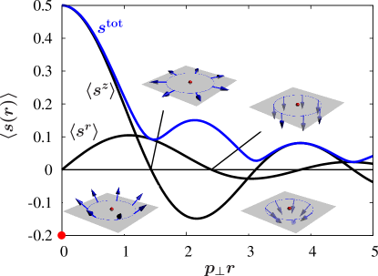
Figure 3: Spin distribution $\langle 1_{{p_{\perp}}\tau\mu}|{\bm{s}}({\bm{x}}_{\perp})|1_{{p_{\perp}}\tau\mu}\rangle=\langle{\bm{s}}(r)\rangle$, Eq. (15) along radial direction with $\tau=\bar{1}$ and $\vartheta=0.9\pi$. $\langle s^{r}\rangle[\langle s^{z}\rangle]$ is the radial [z] component. The blue line is the “total” spin $s^{\rm tot}=\sqrt{\langle s^{r}\rangle^{2}+\langle s^{z}\rangle^{2}}$. Blue arrows show schematic spin distributions at a fixed radius $r$. Thick red dots indicate the impurity location at the origin ${\bm{x}}_{0}=(0,0,0)$.

The Hamiltonian (16) appears to describe a magnetic impurity coupled to two conduction bands (channels) labeled by the helicity index $\tau=\pm 1$. However, this is not actually the case as can be easily demonstrated by converting $H_{\rm ef}$ to the energy representation. We shall consider only energies within the bandgap, $-\Delta\leqslant\epsilon\leqslant\Delta$ and assume that $\pi/2<\vartheta\leqslant\pi$, so $\cos\vartheta\leqslant 0$. There is a one-to-one correspondence between $\tau$ and energy (i.e. helicity of the state and its energy in the upper or lower Dirac cone). From Eqs. (9) and (11) it follows that $\tau=+1(-1)$ corresponds to energies $\epsilon<-\Delta\sin\vartheta$ ($\epsilon>-\Delta\sin\vartheta$). Since $q_{{{\bm{p}}_{\perp}}\tau}$ and $\epsilon_{{{\bm{p}}_{\perp}}\tau}$ depend only on the product $\tau p_{\perp}$,

$$q(\epsilon)=\frac{\Delta+\epsilon\sin\vartheta}{v|\cos\vartheta|}.$$ (17)

Notice that $q(\epsilon)\neq 0$ for all $\epsilon$ within the gap. Next we derive the density of states (DOS) $g_{\tau}(\epsilon)$. For $\tau=+1$ one has $\frac{1}{A}\sum_{p_{\perp}}=\int_{-\Delta\sin\vartheta}^{-\Delta}d\epsilon(\epsilon+\Delta\sin\vartheta)/2\pi v^{2}\cos^{2}\vartheta=\int^{-\Delta\sin\vartheta}_{-\Delta}d\epsilon\,\,g_{+}(\epsilon)$. Similarly for $\tau=-1$: $\frac{1}{A}\sum_{p_{\perp}}=\int_{-\Delta\sin\vartheta}^{\Delta}d\epsilon\,\,g_{-}(\epsilon)$ with $g_{-}(\epsilon)=(\epsilon+\Delta\sin\vartheta)/2\pi v^{2}\cos^{2}\vartheta$. Hence for all energies

$$g(\epsilon)=\frac{|\epsilon+\Delta\sin\vartheta|}{2\pi v^{2}\cos^{2}\vartheta}.$$ (18)

Finally, we introduce new operators $a_{\epsilon\mu}=a_{p_{\perp}(\epsilon)\tau\mu}/\sqrt{g(\epsilon)}$ with anticommutation relations $\{a^{\dagger}_{\epsilon_{\prime}\mu^{\prime}},a_{\epsilon\mu}\}=\delta_{\mu^{\prime}\mu}\delta(\epsilon^{\prime}-\epsilon)$ which allow us to reduce $H_{\rm ef}$ to a single-channel form

$$\frac{H_{\rm ef}}{A}= \int_{-\Delta}^{\Delta}d\epsilon\,\,\epsilon\,a^{\dagger}_{\epsilon\mu}a_{\epsilon\mu}+\frac{1}{2}J_{K}{\bm{S}}\cdot\int_{-\Delta}^{\Delta}d\epsilon^{\prime}\int_{-\Delta}^{\Delta}d\epsilon\times$$

$$\times [g(\epsilon^{\prime})g(\epsilon)q(\epsilon^{\prime})q(\epsilon)]^{1/2}\,a^{\dagger}_{\epsilon^{\prime}\mu^{\prime}}\bigl{(}\sin\vartheta\,{\bm{\sigma}}^{\perp}\!+\sigma^{z}{\bm{e}}_{z}\bigr{)}_{\mu^{\prime}\mu}a_{\epsilon\mu}.$$

This reduction from a two-channel form (16) occurs because of the unique correspondence between energy and helicity peculiar to surface states.

V Unconventional Kondo Physics

The Hamiltonian (16) describes a Kondo impurity model with an anisotropic ($XXZ$) exchange coupling and a DOS (18) that can vanish at the Fermi level, $\epsilon=0$, if the BC $\vartheta=\pi$ is satisfied. In this limit two effects simultaneously ensure that the Kondo screening does not occur, and the impurity spin effectively decouples from the surface metal. First, from numerical renormalization group calculations, for linearly vanishing DOS and particle-hole symmetry the critical Kondo coupling does not exist Gonzalez-Buxton and Ingersent (1998). It is worth noting that this behavior is not captured by the standard mean field theories Withoff and Fradkin (1990). Second, in our system the spin-flip scattering is proportional to $\sin\vartheta$ and therefore disappears at $\vartheta=\pi$. This effect is already present at the mean field level. Hence the decoupling of the impurity from the metallic surface states at $\vartheta=\pi$ is inexorably linked to the anisotropy of the spin scattering stemming from the bulk band structure.

For $\frac{\pi}{2}<\vartheta<\pi$ there is a finite DOS (18) at the Fermi surface, and for temperature $T$ below a characteristic Kondo scale $T_{K}$, the impurity spin is screened Cox and Zawadowski (1999); Hewson (1997). This Kondo effect occurs due to the orbital motion of conduction electrons [Fig. 4(a)] unlike the conventional case when the impurity is screened only by itinerant spins [Fig. 4(b)]. More precisely, the impurity spin forms a singlet with the total angular momentum ${\bm{j}}$ of the surface states. This unconventional mechanism for the Kondo screening originates from the strong SOI that couples spin and orbital momentum of electrons in TIs.

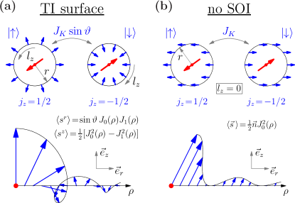
Figure 4: Panel (a) Upper plot: Spin-flip scattering processes leading to the Kondo effect. The red [blue] arrows denote impurity spin at ${\bm{x}}_{\perp}=0$ [local spin (15) in the conduction band at a distance $|{\bm{x}}_{\perp}|=r$ from the origin]. The impurity spin is screened by the orbital degrees of freedom (coupled flips of the electron spin and orbital angular momentum $l_{z}$). The lower plot shows a spiral spin structure (15) along a radial direction ($\rho={p_{\perp}}r$) away from the impurity. (b) Same as in panel (a) but for a conventional metal without SOI. Only conduction electrons in the $s$-wave state couple to the impurity and the orbital angular momentum does not participate in the Kondo screening. The spin direction (along an arbitrary direction ${\bm{n}}$) does not depend on the radial position.

In the following we would like to address the physical manifestations of this unconventional Kondo effect. We first demonstrate the appearance of a transverse spin linear response to a longitudinal external magnetic field. We next consider the effect of temperature and study the dependence of the Kondo temperature on the electronic surface properties parameterized by $\vartheta$. Although we focus on the model (16) obtained in the context of TIs, results of the present section are applicable to Kondo physics in any two-dimensional metal with SOI.

V.1 Transverse local magnetic response

The simplest manifestation of the spin-orbital nature of the Kondo effect on a TI surface can be found in the zero temperature ($T=0$) linear response to a weak magnetic field ${\bm{h}}$ acting on the impurity. Assuming that ${\bm{h}}=h{\bm{e}}_{z}$ points perpendicular to the surface, the field correction to the model (16) is

$$H_{\rm mag}=-hS^{z}.$$

According to Eq. (15), surface states with $\mu={\uparrow}$ and ${\downarrow}$ correspond to different (opposite) radial spin distributions. In the Kondo singlet state both configurations are equally probable and the total spin in the $xy$-plane vanishes. However, in an applied magnetic field the impurity spin is weakly polarized creating a population imbalance of electrons with different $\mu$’s. This imbalance results in a transverse local (i.e. at a fixed distance from the impurity) spin polarization in the conduction band, see Fig. 5(a).

To calculate the field-induced transverse magnetization we use the standard variational approach Yosida (1966); Isaev et al. (2011) for the Kondo problem, and assume that $\vartheta<\pi$ so that all $\tau=+1$ states are filled and the Fermi level lies in the $\tau=-1$ cone in Fig. 1(d). At weak coupling $\frac{J_{K}\Delta^{2}}{v^{3}}\ll 1$ one needs to keep only $\tau=-1$ terms in Eq. (16), hence in the rest of this Subsection we will omit $\tau$ in the subscripts. The variational wavefunction has the form Ishii and Yosida (1967):

$$|\psi_{0}\rangle=\sum_{{p_{\perp}}\geqslant k_{F}}[{\cal A}_{p_{\perp}}\chi^{s}_{\mu\alpha}+{\cal B}_{p_{\perp}}\chi^{t}_{\mu\alpha}]a^{\dagger}_{{p_{\perp}}\mu}|{\rm FS}\rangle\otimes|\alpha\rangle,$$ (19)

where $k_{F}=\frac{\Delta\sin\vartheta}{v|\cos\vartheta|}$ is the Fermi momentum, and $|{\rm FS}\rangle$ and $|\alpha\rangle$ are the Fermi sea and impurity spin states ($\alpha={\uparrow},{\downarrow}$) respectively. There is an implicit summation over spin indices. The two terms in (19) correspond to singlet ($\chi^{s}$) and triplet ($\chi^{t}$) components with $\chi^{s,t}_{\mu\alpha}=\frac{1}{\sqrt{2}}(\delta_{\mu{\uparrow}}^{\alpha{\downarrow}}\mp\delta_{\mu{\downarrow}}^{\alpha{\uparrow}})$. The latter satisfy the relations $\chi^{s}_{\mu\alpha}\chi^{s}_{\mu\alpha}=\chi^{t}_{\mu\alpha}\chi^{t}_{\mu\alpha}=1$, $\chi^{s}_{\mu\alpha}\chi^{t}_{\mu\alpha}=0$, and $S^{z}_{\alpha\beta}\chi^{s}_{\mu\beta}=\frac{1}{2}\chi^{t}_{\mu\alpha}$. The state (19) is normalized according to $\langle\psi_{0}|\psi_{0}\rangle=\sum_{{p_{\perp}}\geqslant k_{F}}\bigl{(}|{\cal A}_{p_{\perp}}|^{2}+|{\cal B}_{p_{\perp}}|^{2}\bigr{)}=1$.

The amplitudes ${\cal A}_{p_{\perp}}$ and ${\cal B}_{p_{\perp}}$ are variational parameters determined by minimizing the functional ${\cal F}=\langle\psi_{0}|H_{\rm ef}+H_{\rm mag}|\psi_{0}\rangle-(E_{\rm FS}-\lambda)\langle\psi_{0}|\psi_{0}\rangle$, where $\lambda$ is the Lagrange multiplier that plays the role of an energy shift due to the Kondo screening. To the first order in $h$, a straightforward calculation yields

$$\begin{pmatrix}{\cal A}_{p_{\perp}}\\ {\cal B}_{p_{\perp}}\end{pmatrix}=\frac{J_{K}(1+2\sin\vartheta)}{4A}\frac{c\sqrt{q_{p_{\perp}}}}{(\epsilon_{p_{\perp}}+\lambda)^{2}}\begin{pmatrix}\epsilon_{p_{\perp}}+\lambda\\ -h/2\end{pmatrix},$$

with ${p_{\perp}}\geqslant k_{F}$ and $c=\sum_{{p_{\perp}}\geqslant k_{F}}\sqrt{q_{p_{\perp}}}A_{p_{\perp}}$. The eigenvalue $\lambda$ is determined from the non-linear equation

$$1=\frac{J_{K}(1+2\sin\vartheta)}{4A}\sum_{{p_{\perp}}\geqslant k_{F}}\frac{q_{p_{\perp}}}{\epsilon_{p_{\perp}}+\lambda}.$$ (20)

At weak coupling the sum can be computed as $\frac{1}{A}\sum_{p_{\perp}}\ldots=\int_{0}^{\Delta}d\epsilon\,\,\frac{g(\epsilon)q(\epsilon)}{\epsilon+\lambda}\approx q(0)g(0)\ln\frac{\Delta}{\lambda}$ [$q(\epsilon)$ is given in Eq. (17)] which means that $\ln\frac{\lambda}{\Delta}\approx-8\pi v^{3}|\cos^{3}\vartheta|/\Delta^{2}J_{K}\sin\vartheta(1+2\sin\vartheta)$. Then, the normalization constant $c$ is given by $c^{2}=\frac{A\lambda}{g(0)q(0)}\bigl{[}\frac{4}{J_{K}(1+2\sin\vartheta)}\bigr{]}^{2}$.

If, as is commonly done, one identifies the energy shift $\lambda$ with the Kondo temperature $T_{K}$, we find that, as $\vartheta\rightarrow\pi$, $T_{K}$ vanishes exponentially as $T_{K}\sim\Delta\exp\bigl{[}-8\pi v^{3}/\Delta^{2}J_{K}(\pi-\vartheta)\bigr{]}$. Note, however, that in this approach for a finite DOS at the Fermi level the variational energy shift does not vanish when spin-flip processes are suppressed. Consequently, in next subsection we take this effect into account and define the Kondo temperature using the slave-boson method.

The field-induced transverse spin distribution in the ground state $|\psi_{0}\rangle$ is straightforwardly obtained using Eq. (24) and the discussion in Sec. IV:

$$\langle\psi_{0}|s^{r}({\bm{x}}_{\perp})|\psi_{0}\rangle= \frac{\sin\vartheta}{A}\sigma^{x}_{mn}\times$$

$$\times\sum_{{p^{\prime}_{\perp}}{p_{\perp}}\geqslant k_{F}} \sqrt{q_{p^{\prime}_{\perp}}q_{p_{\perp}}}{\cal A}_{p^{\prime}_{\perp}}{\cal B}_{p_{\perp}}J_{n}({p^{\prime}_{\perp}}r)J_{m}({p_{\perp}}r),$$

with $n,m=0$ and $1$. With the aid of the above expressions for $\lambda$, $c$, ${\cal A}_{p_{\perp}}$ and ${\cal B}_{p_{\perp}}$, we finally arrive at

$$\langle\psi_{0}|s^{r}({\bm{x}}_{\perp})|\psi_{0}\rangle=-\frac{4h\sin\vartheta}{(1+2\sin\vartheta)J_{K}}J_{0}(k_{F}r)J_{1}(k_{F}r),$$

where we also employed a weak-coupling approximation for the energy integrals $\int_{0}^{\Delta}d\epsilon f(\epsilon)/(\epsilon+\lambda)^{n}\approx f(0)\int_{0}^{\Delta}d\epsilon/(\epsilon+\lambda)^{n}$ ($f$ is a smooth function and $n\geqslant 0$ is an integer). Due to the structure of the variational state (19) the spin distribution is identical up to a prefactor to Eq. (15) with ${p_{\perp}}=k_{F}$ [see also Fig. 3].

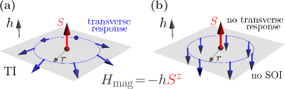
Figure 5: Panel (a) Schematic plot of the transverse magnetic response on a TI surface. A magnetic field $h$ applied normal to the surface causes a radial electron spin polarization. (b) Same as panel (a), but for the Kondo effect in a usual two-dimensional metal without SOI. There is only longitudinal magnetic response.

The transverse magnetic response, i.e. nonzero $\langle s^{r}\rangle\sim h$, can be viewed as a variation of the Edelstein effect Aronov and Lyanda-Geller (1989); Edelstein (1990): an applied magnetic field creates an imbalance of different orbital angular momentum states that couple to the impurity, which in turn induces a radial spin polarization. This phenomenon exists only due to the SOI and is absent in metals without SOI [see Fig. 5(b)]. Therefore, by studying the spatial structure of the Kondo resonance, for example by spin-polarized STM, one can differentiate between topologically non-trivial and trivial states of matter. Field-induced radial spin spirals similar to Figs. 4(a) and 5(a) were reported in Ref. Chirla et al., 2013 in connection to Kondo screening of magnetic impurities on gold surfaces with a weak Rashba SOI $\alpha_{R}$. In that work, the transverse susceptibility $\kappa_{\perp}=\langle s^{r}\rangle/h\sim\alpha_{R}$. Our results deal with an opposite limit of strong SOI and hence $\kappa_{\perp}$ depends only on $J_{K}$ and the boundary parameter $\vartheta$.

In the absence of an external field $h$, the ground state wavefunction (19) is an $SU(2)$-singlet, despite the $XXZ$ anisotropy of the Kondo model (16). This is an example of the general irrelevance of exchange anisotropies for the Kondo physics Cox and Zawadowski (1999). However, in our case this emergent $SU(2)$ symmetry is quite non-trivial because the impurity spin forms a singlet with the total angular momentum of the surface electrons [see Fig. 4(a)]. Coupling to the orbital motion ensures that this singlet-formation is the physical mechanism responsible for the Kondo resonance even when electron spins are quenched by the strong SOI.

V.2 Slave-boson mean-field approach

In the previous Subsection we assumed that for any $\vartheta<\pi$ the impurity is screened by surface electrons with only one helicity $\tau=-1$. Here we verify this conjecture by studying the model in Eq. (16) within the slave boson mean-field approach Hewson (1997); Orignac and Burdin (2013). This analysis also provides an extension of our previous results to finite temperature.

First we introduce a pseudofermion representation of the local spin ${\bm{S}}=\frac{1}{2}f^{\dagger}_{\mu}{\bm{\sigma}}_{\mu\nu}f_{\nu}$ with the constraint $\sum_{\mu}f^{\dagger}_{\mu}f_{\mu}=1$. In this language the interaction term in $H_{\rm ef}$ can be written in a compact form

$$H_{\rm ef}= -J_{K}\sin\vartheta\hat{\chi}^{\dagger}_{0}\hat{\chi_{0}}+J_{K}\frac{1-\sin\vartheta}{2}\hat{\bm{\chi}}^{\dagger}_{\perp}\cdot\hat{\bm{\chi}}_{\perp}-$$

$$-J_{K}\frac{1-2\sin\vartheta}{4}\sum_{\begin{subarray}{c}{p^{\prime}_{\perp}}\tau^{\prime}\\ {p_{\perp}}\tau\end{subarray}}Q^{{p^{\prime}_{\perp}}\tau^{\prime}}_{{p_{\perp}}\tau}a^{\dagger}_{{p^{\prime}_{\perp}}\tau^{\prime}\mu}a_{{p_{\perp}}\tau\mu}.$$ (21)

The slave bosons are defined as Viola Kusminskiy et al. (2008): $\hat{\chi}_{l}=\frac{1}{\sqrt{2A}}\sum_{{p_{\perp}}\tau}\sqrt{q_{{p_{\perp}}\tau}}f^{\dagger}_{\mu}\sigma^{l}_{\mu\nu}a^{\;}_{{p_{\perp}}\tau\nu}$ with $l=0,1,2,3$ and $\sigma^{0}_{\mu\nu}=\delta_{\mu\nu}$ [see Fig. 6]. Notice, that the zero energy in Eq. (21) is chosen such that it eliminates $\hat{\chi}_{z}$, which is necessary since energies of the states with condensed $\chi_{0}$ and $\chi_{z}$ bosons (see below) are only different when spin-flip scattering is present. This procedure adds a potential scattering term that preserves the impurity spin and is therefore irrelevant for the Kondo physics [cf Ref. Orignac and Burdin, 2013].

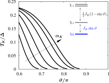
Figure 6: Kondo temperature, computed from the Nagaoka-Suhl equation (22), as a function of the BC angle $\vartheta$ [see Eq (8)]. The arrow shows increasing values of the dimensionless Kondo coupling $\alpha_{K}=J_{K}\Delta^{2}/2\pi v^{3}=0.05$, $0.1$, $0.2$, $0.4$, $0.7$, $1.0$. Inset: Energies involved in the Hamiltonian (21). The blue color indicates the condensed slave boson $\chi_{0}$.

The mean-field appoximation amounts to treating the pseudofermion constraint on the average via a chemical potential $E_{f}$, and assuming that the ground state corresponds to condensation of the $\chi_{0}$ boson, i.e. $\langle\hat{\bm{\chi}}_{\perp}\rangle=0$ but $\langle{\hat{\chi}}_{0}\rangle=\chi_{0}\neq 0$. The mean-field Hamiltonian,

$$H_{\rm MF}= \sum_{{p_{\perp}}\tau\mu}\epsilon_{{p_{\perp}}\tau}a^{\dagger}_{{p_{\perp}}\tau\mu}a_{{p_{\perp}}\tau\mu}-E_{f}\sum_{\mu}f^{\dagger}_{\mu}f_{\mu}-$$

$$-\frac{J_{K}\sin\vartheta}{2A}\sum_{{p_{\perp}}\tau\mu}\sqrt{q_{{p_{\perp}}\tau}}\bigl{(}\chi_{0}a^{\dagger}_{{p_{\perp}}\tau\mu}f_{\mu}+{\rm h.c.}\bigr{)},$$

can be diagonalized using the equations of motion method for retarted Green functions Zubarev (1960); Nagaoka (1965) which, for fermions, are defined as $\langle\langle A;B\rangle\rangle=-{\rm i}\theta(t-t^{\prime})\langle\{A(t),B(t^{\prime})\}\rangle$ [$\theta(x)$ is the Heaviside step function]. We will need three types of Green functions: $\langle\langle a^{\;}_{{p_{\perp}}\tau\mu};a^{\dagger}_{{p^{\prime}_{\perp}}\tau^{\prime}\mu}\rangle\rangle$, $\langle\langle f^{\;}_{\mu};f^{\dagger}_{\mu}\rangle\rangle$, and $\langle\langle f^{\;}_{\mu};a^{\dagger}_{{p_{\perp}}\tau\mu}\rangle\rangle$. A direct calculation yields:

$$\langle a^{\;}_{{p_{\perp}}\tau\mu}; a^{\dagger}_{{p^{\prime}_{\perp}}\tau^{\prime}\mu}\rangle_{\omega}=\frac{\delta_{{p^{\prime}_{\perp}}{p_{\perp}}}^{\tau^{\prime}\tau}}{\omega-\epsilon_{{p_{\perp}}\tau}}-$$

$$-\frac{J_{K}\sin\vartheta}{\sqrt{2A}}\frac{\chi_{0}\sqrt{q_{{p_{\perp}}\tau}}}{\omega-\epsilon_{{p_{\perp}}\tau}}\langle f^{\;}_{\mu};a^{\dagger}_{{p^{\prime}_{\perp}}\tau^{\prime}\mu}\rangle_{\omega}$$

$$\langle f^{\;}_{\mu}; a^{\dagger}_{{p_{\perp}}\tau\mu}\rangle_{\omega}=-\frac{J_{K}\sin\vartheta\chi_{0}^{*}\sqrt{q_{{p_{\perp}}\tau}}}{\sqrt{2A}(\omega-\epsilon_{{p_{\perp}}\tau})\bigl{[}\omega+E_{f}-\Omega(\omega)\bigr{]}},$$

where we introduced the Fourier transform $\langle\langle A;B\rangle\rangle=\frac{1}{2\pi}\int_{-\infty}^{\infty}d\omega\,{\rm e}^{-{\rm i}\omega(t-t^{\prime})}\langle A;B\rangle_{\omega}$, and the impurity self-energy

$$\Omega(\omega)=\frac{|J_{K}\sin\vartheta\chi_{0}|^{2}}{2A}\sum_{{p_{\perp}}\tau}\frac{q_{{p_{\perp}}\tau}}{\omega-\epsilon_{{p_{\perp}}\tau}}.$$

The mixed Green function $\langle f^{\;}_{\mu};a^{\dagger}_{{p_{\perp}}\tau\mu}\rangle_{\omega}$ allows us to construct the self-consistency equation for $\chi_{0}$:

$$\chi_{0}^{*}= \frac{1}{\sqrt{2A}}\sum_{{p_{\perp}}\tau\mu}\sqrt{q_{{p_{\perp}}\tau}}\langle a^{\dagger}_{{p_{\perp}}\tau\mu}f^{\;}_{\mu}\rangle=$$

$$=\frac{1}{\sqrt{2A}}\sum_{{p_{\perp}}\tau\mu}\sqrt{q_{{p_{\perp}}\tau}}\int d\omega\,{\cal A}_{{p_{\perp}}\tau\mu}(\omega),$$

with the spectral function

$${\cal A}_{{p_{\perp}}\tau\mu}(\omega)=\frac{{\rm i}}{2\pi}\frac{\langle f^{\;}_{\mu};a^{\dagger}_{{p_{\perp}}\tau\mu}\rangle_{\omega+{\rm i}0}-\langle f^{\;}_{\mu};a^{\dagger}_{{p_{\perp}}\tau\mu}\rangle_{\omega-{\rm i}0}}{{\rm e}^{\omega/T}+1}.$$

At the Kondo temperature $T_{K}$, defined by $E_{f}(T_{K})=\Omega(T_{K})=0$, the above self-consistency condition reduces to the Nagaoka-Suhl equation

$$1=-\frac{J_{K}\sin\vartheta}{A}\,\,{\rm P.V.}\sum_{{p_{\perp}}\tau}\frac{q_{{p_{\perp}}\tau}}{\epsilon_{{p_{\perp}}\tau}\bigl{(}{\rm e}^{\epsilon_{{p_{\perp}}\tau}/T_{K}}+1\bigr{)}},$$ (22)

where ${\rm P.V.}$ indicates the Cauchy principal value. This expression generalizes the Yosida equation (20) for the case where both helicities $\tau$ are allowed to participate in the Kondo screening.

For $\vartheta$ sufficiently distinct from $\pi$ and weak coupling we only need to consider conduction band states near the Fermi energy. All of them have the same helicity due to the one-to-one correspondence between $\tau=\pm 1$ and energy leading to the helicity-independent DOS (18). This fact justifies our assumptions made in the previous Subsection.

Beyond weak coupling, the sum in (22) can be computed numerically using Eqs. (17) and (18) for $q(\epsilon)$ and $g(\epsilon)$. The dependence of the Kondo temperature on $\vartheta$ is shown in Fig. 6. Asymptotically, for $\vartheta\to\pi$, the Kondo temperature $T_{K}\sim\Delta\exp\bigl{[}-2\pi v^{3}/\Delta^{2}J_{K}(\pi-\vartheta)^{2}\bigr{]}$ is exponentially suppressed, albeit its functional behavior is different from that obtained using the variational approach. Since at $\vartheta=\pi$, the $XY$ term in (16) vanishes, there is no critical Kondo coupling that would yield a finite $T_{K}$ at this point [cf. Ref. Withoff and Fradkin, 1990].

VI Discussion

In the present work we advocated the use of magnetic probes to test and tune the unconventional phenomena at topological insulator surfaces. We showed that physical characteristics and quantum numbers of the surface states are quite sensitive to surface properties encoded in boundary conditions for electron wavefunctions, as well as the structure of bulk Bloch bands. Moreover, we demonstrated how the combination of spin-orbit interaction and non-trivial boundary conditions leads to an unconventional Kondo screening of dilute magnetic impurities on the surface of a 3D topological insulator.

We considered a localized spin $S=\frac{1}{2}$ (magnetic) impurity atom deposited on the $(111)$ surface of a ${\rm PbTe}$-class narrow-band semiconductor, and derived a low-energy effective theory that governs the coupling of this local spin to surface electrons taking into account the full 3D structure of surface-state wavefunctions. The resulting Kondo impurity model is spatially non-local and anisotropic [$XXZ$-like, see Eq. (16)]. Interestingly, both of these features are controlled by parameters defined by the boundary conditions, in our case $\vartheta$, that determine the magnitude of the particle-hole asymmetry at the surface [see Fig. 1(d)]. Specifically, at the particle-hole symmetric point $\vartheta=\pi$ the $XY$ component of the Kondo exchange interaction vanishes, signalling an instability of the Kondo screened ground state (for any amount of surface gating) due to the lack of spin-flip processes.

When the particle-hole symmetry is broken by the boundary conditions, we find that the impurity spin is fully screened by the surface electrons, in agreement with earlier works Zitko (2010); Feng et al. (2010); Orignac and Burdin (2013); Mitchell et al. (2013); Tran and Kim (2010); Žitko and Bonča (2011). However, unlike the conventional Kondo effect Hewson (1997), here the local spin forms a singlet with the total angular momentum of itinerant electrons (as opposed to only their spin) and is screened mainly by the orbital electronic degrees of freedom. This effect originates in the strong spin-orbit interaction that underpins the helical structure of the surface states, and manifests itself in a transverse spin response: A weak, normal to the surface, magnetic field induces an in-plane electron spin polarization [see Fig. 5(a)] which locally resembles a $q=1$ magnetic vortex (see Ref. Nomura and Nagaosa, 2010) with itinerant spins aligning along the radial direction.

The sensitivity of the Kondo screening to specific surface properties shows that it is impossible to provide a universal theory of topological insulator surface states based solely on topological arguments Qi and Zhang (2011); Hasan and Kane (2010) without involving knowledge of the boundary conditions for the Bloch states (see Sec. II and Ref. Isaev et al., 2011), and, as elaborated in the present work, the specific bulk band structure. Most importantly, the latter defines the set of relevant effective operators that parameterize the surface theory. Indeed, in Sec. III we demonstrated that for a ${\rm Bi_{2}Se_{3}}$-like tetragonal material the form of the surface Kondo interaction is completely different (isotropic, $XXX$-like) than in cubic ${\rm PbTe}$-like systems (anisotropic, $XXZ$-like).

This physical non-universality of topological surface states can be exploited in experimental studies of topological insulators, for instance to control the surface spin polarization with external electric and magnetic fields. Although we focused on magnetic impurities, our analysis can be generalized to any magnetic interaction, e.g. the Zeeman coupling of surface electrons to external fields. For ${\rm Bi_{2}Se_{3}}$-like materials, the only effect of an in-plane magnetic field is to shift (neglecting the Fermi surface warping) the Dirac cone in the Brillouin zone Fu (2009). However, in ${\rm PbTe}$-like crystals with a particle-hole symmetric boundary ($\vartheta=\pi$) such field does not couple to surface states at all. In general, this coupling can be tuned by surface manipulation. The above result shows a convenient way of discriminating between different types of topological insulators by using interactions of surface states with external magnetic probes.

The transverse spin structures in Fig. 5(a) can be observed in scanning tunneling microscopy measurements of the local spin-polarized density of states around the impurity, or nuclear magnetic resonance experiments. This predicted effect is not peculiar to topological insulators and should in fact exist in any strong spin-orbit coupled metallic host. A similar idea of probing the local spin polarization around magnetic impurities in a metal without spin-orbit interaction, i.e. the analysis of the Kondo screening cloud, was discussed before Affleck (2010). Unlike our analysis, in that work the magnetic field induced only a longitudinal (and no transverse) spin polarization [Fig. 5(b)].

Finally, we comment on the role of impurity charge fluctuations in multiband Dirac-like materials with strong spin-orbit coupling. The standard Kondo impurity Hamiltonian is typically derived from the Anderson impurity model via a Schrieffer-Wolff (SW) transformation assuming that charge fluctuations at the impurity get suppressed Hewson (1997). In the absence of spin-orbit interaction, the virtual transitions included in the SW transformation preserve the electron spin quantum number. The effective Kondo exchange then depends on momentum only via energy, and near the Fermi level can be approximated by a constant value. This situation may change in a spin-orbit coupled system when the electron transitions between local and itinerant states are accompanied by a spin-flip. For a ${\rm PbTe}$-like host these processes can be captured with a modified 3D Anderson impurity model

$$H_{\rm AIM}\!=\!H_{0}+\frac{1}{\sqrt{N}}\sum_{\bm{p}}\bigl{[}V^{c}_{\alpha\beta}({\bm{p}})c^{\dagger}_{{\bm{p}}\alpha}d^{\;}_{\beta}+V^{v}_{\alpha\beta}({\bm{p}})h^{\dagger}_{{\bm{p}}\alpha}d^{\;}_{\beta}+{\rm h.c.}\bigr{]},$$

written in terms of the fermion operators $d^{\dagger}_{\alpha}$, $c^{\dagger}_{{\bm{p}}\alpha}$ and $h^{\dagger}_{{\bm{p}}\alpha}$ that create electrons in the impurity orbital, conduction and valence band, respectively. $H_{0}=H_{\rm D}+H_{d}$, with $H_{\rm D}$ from Eq. (1) and $H_{d}$ representing the self-energy of the localized electrons. The matrix amplitudes $V^{c}_{\alpha\beta}$ and $V^{v}_{\alpha\beta}$ describe hybridizations of the local impurity level with electrons in the conduction and valence bands.

A phenomenological form of these amplitudes can be obtained from general symmetry considerations. We require that $H_{\rm AIM}$ has the same symmetries as the non-interacting Dimmock model $H_{\rm D}$, in particular, time-reversal invariance and symmetry w.r.t. spatial inversion ${\cal P}$. The former demands that $V^{c}$ and $V^{v}$ contain spin (via the Pauli matrices) and momentum in even power combinations, e.g. $p^{2}$ or ${\bm{\sigma}}\cdot{\bm{p}}$. The inversion symmetry dictates which of these terms actually occur in each hybridization amplitude. Under ${\cal P}$, local fermions are invariant $d_{\alpha}\stackrel{{\scriptstyle\cal P}}{{\to}}d_{\alpha}$, while conduction and valence band electrons transform as Berestetskii et al. (1982) $c_{{\bm{p}}\alpha}\stackrel{{\scriptstyle\cal P}}{{\to}}c_{-{\bm{p}}\alpha}$ and $h_{{\bm{p}}\alpha}\stackrel{{\scriptstyle\cal P}}{{\to}}-h_{-{\bm{p}}\alpha}$. This means that $V^{c}$ ($V^{v}$) is an even (odd) function of ${\bm{p}}$: $V^{c}({\bm{p}})=V_{c0}+V_{c1}p^{2}+\cdots$ and $V^{v}({\bm{p}})=V_{v1}({\bm{\sigma}}\cdot{\bm{p}})+\cdots$. To lowest order in momentum, $V^{c}$ can be taken ${\bm{p}}$-independent: $V^{c}_{\alpha\beta}({\bm{p}})\approx V_{c0}\delta_{\alpha\beta}$. On the other hand, $V^{v}_{\alpha\beta}({\bm{p}})\approx V_{v1}({\bm{\sigma}}_{\alpha\beta}\cdot{\bm{p}})$ has a $p$-wave structure and is spatially non-local. This result differs from the calculations of Refs. Lü et al., 2013; Kuzmenko et al., 2014 which used constant values for both amplitudes $V^{c}$ and $V^{v}$.

Applying the SW transformation to $H_{\rm AIM}$ yields a modified effective Kondo model: apart from the local exchange coupling $J_{K}$, there are essentially non-local corrections that include $p$-wave couplings between conduction electrons and the local impurity spin. We considered the simplest version in this paper and leave the more complex situation for a future investigation.

VII Acknowledgements

L.I. was supported by the NSF (PIF-1211914 and PFC-1125844), AFOSR, AFOSR-MURI, NIST and ARO individual investigator awards, and also in part by ICAM. I.V. acknowledges support from NSF Grants DMR-1105339 and DMR-1410741.

Appendix A Self-adjoint extensions of the Dirac and Dimmock Hamiltonians in the half-space

Given a linear bounded operator ${\bm{O}}$, its adjoint ${\bm{O}}^{\dagger}$ is defined as $\langle\psi|{\bm{O}}^{\dagger}\phi\rangle=\langle{\bm{O}}\psi|\phi\rangle$ for all vectors $|\psi\rangle$ and $|\phi\rangle$ in the Hilbert space ${\cal H}$. Moreover, ${\bm{O}}$ is symmetric (or Hermitian) if $\langle\psi|{\bm{O}}\phi\rangle=\langle{\bm{O}}\psi|\phi\rangle$ or ${\bm{O}}^{\dagger}={\bm{O}}$ for all vectors $|\psi\rangle$ and $|\phi\rangle$. The set of all vectors $|\phi\rangle$ for which ${\bm{O}}|\phi\rangle$ is defined is called the domain of the operator ${\bm{O}}$. For a bounded symmetric operator ${\bm{O}}$ its domain covers the entire space: ${\cal D}({\bm{O}})={\cal D}({\bm{O}}^{\dagger})={\cal H}$.

On the other hand, if a linear operator ${\bm{H}}$ is unbounded its domain does not necessarily coincide with that of its adjoint. One can make these two domains coincide by defining them appropriately. If ${\cal D}({\bm{H}}^{\dagger})$ contains ${\cal D}({\bm{H}})$, and in ${\cal D}({\bm{H}})$ the two operators are the same, then we say that ${\bm{H}}^{\dagger}$ is an extension of ${\bm{H}}$. A symmetric operator ${\bm{H}}$ with a dense domain is self-adjoint whenever ${\cal D}({\bm{H}})={\cal D}({\bm{H}}^{\dagger})$ Ahari et al. (2015).

In this section we prove that the Dirac Hamiltonian (7) in the half-space $z\geqslant 0$ is self-adjoint in the domain of wavefunctions satisfying the BC (8) (the following analysis can also be seen as another derivation of this BC). We also determine self-adjoint extensions (SAEs) of the Dimmock Hamiltonian (1) in the half-space. This constitutes a crucial step to discussing and analyzing surface or interface phenomena that is physically observable.

The general theory of self-adjoint extensions can be found, for instance, in Ref. Gitman et al., 2012. Its practical application to an operator $H$, however, is rather straightforward Ahari et al. (2015); Bonneau et al. (2001); Araujo et al. (2004) and was made systematic by von Neumann’s method of deficiency indices. First, one constructs deficiency subspaces of the adjoint operator, i.e. determines eigenfunctions $\psi_{\pm}$ of $H^{\dagger}$ corresponding to eigenvalues $\pm{\rm i}\eta$ with arbitrary $\eta>0$. Dimensions of these subspaces, the deficiency indices $n_{\pm}$, give the number of parameters needed to construct families of possible SAEs: if $n_{+}=n_{-}=n=0$ the operator is already self-adjoint, otherwise ($n>0$) its extensions need to be built. When $n_{+}\neq n_{-}$ the operator cannot be made self-adjoint.

Provided $n_{+}=n_{-}$, the next step is to demand that the positive and negative deficiency subspaces be unitarily related by a $n\times n$ matrix $U$. This matrix is arbitrary and therefore the number of possible SAEs is $n^{2}$. Finally, we require that the combination $\psi_{+}+U\psi_{-}$ belong to the domain of the original operator $H$. This yields BC for the wavefunctions that define the domain in which $H$ is self-adjoint. The arbitrary unitary matrix $U$ represents all possible BCs compatible with $H$ being self-adjoint. One can then consider SAEs that are constrained by additional symmetry conditions, such as time-reversal invariance or parity.

A.1 Dirac Hamiltonian in the half-space $z\geqslant 0$

For purely imaginary eigenvalues $\pm{\rm i}\eta$ of the Hamiltonian (7) it follows that $p_{z}=\pm{\rm i}\sqrt{(\eta^{2}+\Delta^{2})/v^{2}+p_{\perp}^{2}}=\pm{\rm i}\kappa$. To find the corresponding eigenfunctions $\psi_{\pm}$, it is convenient to reduce Eq. (7) to a $2\times 2$ form similar to Eq. (5):

$$H^{(2\times 2)}=v\bigl{(}\sigma^{x}p_{z}-\sigma^{y}\tau p_{\perp}\bigr{)}+\sigma^{z}\Delta,$$

and make a unitary transformation generated by

$$\zeta=\frac{1}{\sqrt{2}}\begin{pmatrix}1&1\\ {\rm i}&-{\rm i}\end{pmatrix}.$$

so that $\zeta^{\dagger}{\bm{\sigma}}\zeta=(\sigma^{y},\sigma^{z},\sigma^{x})$. In this representation:

$$\psi_{\pm}=\begin{pmatrix}\pm{\rm i}\eta-v\tau p_{\perp}\\ \Delta-v\kappa\end{pmatrix}{\rm e}^{-\kappa z},$$

where we dropped the unimportant, for the analysis below, dependence on ${\bm{x}}_{\perp}$ as well as the normalization constant (which is the same for $\psi_{+}$ and $\psi_{-}$). Clearly, this solution exists for any sign of $\pm{\rm i}\eta$, hence the deficiency indices are $n_{+}=n_{-}=1$. By the von Neumann theorem, the Hamiltonian (7) has a single-parameter, $n=1$, family of SAEs. The unitary matrix, connecting $\psi_{+}$ and $\psi_{-}$ is just ${\rm e}^{{\rm i}\lambda}$ with an arbitrary $\lambda$.

Possible SAEs are found in the form of BC for a general wavefunction $\varphi=(\varphi_{1}^{*},\varphi_{2}^{*})^{\dagger}$ from the domain of $H$. The condition that $H$ is self-adjoint if

$$\langle\psi|H\varphi\rangle-\langle H^{\dagger}\psi|\varphi\rangle=-{\rm i}\psi^{\dagger}\alpha^{z}\varphi\bigl{|}_{z=0}=0$$

[$\psi\in{\cal D}(H^{\dagger})$ and we are interested in functions such that ${\cal D}(H)={\cal D}(H^{\dagger})$]. Substituting $\psi=\psi_{+}+{\rm e}^{{\rm i}\lambda}\psi_{-}$, we obtain (note that $\alpha^{z}$ is equivalent to $\sigma^{y}$):

$$\frac{\varphi_{1}}{\varphi_{2}}\biggl{|}_{z=0}=-\frac{v\tau p_{\perp}\cos\lambda/2-\eta\sin\lambda/2}{(\Delta-v\kappa)\cos\lambda/2}=\rho,$$

where $\rho$ is an arbitrary real constant.

As a final step, we would like to recast this BC in a form $B^{\prime}\varphi|_{z=0}=0$ ($\det B^{\prime}=0$). The matrix $B^{\prime}$ can be written as

$$B^{\prime}= b_{1}\begin{pmatrix}b_{2}&b_{2}\rho\\ 1&\rho\end{pmatrix}=\frac{b_{1}}{2}\bigl{[}(b_{2}+\rho)+(b_{2}-\rho)\sigma^{z}+$$

$$\qquad\qquad+(1+b_{2}\rho)\sigma^{x}-{\rm i}(1-b_{2}\rho)\sigma^{y}\bigr{]},$$

with arbitrary real $b_{2}$ (notice that $b_{1}$ is irrelevant). This BC preserves time-reversal and parity invariance of the Dirac Hamiltonian. The BC of Eq. (8) is recovered after inverting the $\zeta$-transformation, i.e. replacing ${\bm{\sigma}}$ with $(\beta,\alpha^{z},-{\rm i}\beta\alpha^{z})$, and taking $b_{1}=2\rho/(1+\rho^{2})$ and $b_{2}=1/\rho$. Then $\sin\vartheta=2\rho/(1+\rho^{2})$ and $\cos\vartheta=(1-\rho^{2})/(1+\rho^{2})$.

A.2 Dimmock Hamiltonian in the half-space $z\geqslant 0$

Similarly to the previous subsection, for the Dimmock model (1), we have:

$$\frac{p_{z}^{2}}{2(m^{*}v)^{2}}=-\biggl{[}1+\frac{\Delta+p^{2}_{\perp}/2m^{*}}{m^{*}v^{2}}\biggr{]}\pm\sqrt{1+\frac{2\Delta-\eta^{2}/m^{*}v^{2}}{m^{*}v^{2}}}.$$

It is straightforward to check that for any values of the parameters $\Delta$ and $p_{\perp}$, there are two normalizable solutions that decay with $z\to\infty$. Therefore, the deficiency indices are $n_{+}=n_{-}=2$, and the self-adjoint extension of Eq. (1) is realized by a four-parametric family of BCs.

Appendix B Surface states in the total angular momentum basis

The eigenvalue problem defined by the Dirac Hamiltonian (7) and its BC (8) has an axial symmetry around the $z$-axis which leads to conservation of the $z$-component of the total angular momentum $j_{z}=l_{z}+\frac{1}{2}\Sigma^{z}$ ($l_{z}$ is the orbital angular momentum). Here we will employ this symmetry to construct surface states with a definite value of $j_{z}$, and derive their spin structure (15) and coupling to the impurity [see Eq. (16)].

We will work in cylindrical coordinates $(r,\varphi,z)$ with $0\leqslant r<\infty$ and $0\leqslant\varphi<2\pi$, related to the Cartesian basis in Fig. 1(a) via $x=r\cos\varphi$ and $y=r\sin\varphi$. The vector product $[{\bm{\sigma}}\times{{\bm{p}}_{\perp}}]_{z}$ entering the tensor spin operator $T_{z}$ [see Eq. (2)] has the form

$$[{\bm{\sigma}}\times{{\bm{p}}_{\perp}}]_{z}=\begin{pmatrix}0&{\rm e}^{-{\rm i}\varphi}\bigl{(}\frac{\partial}{\partial r}+\frac{l_{z}}{r}\bigr{)}\\ {\rm e}^{{\rm i}\varphi}\bigl{(}-\frac{\partial}{\partial r}+\frac{l_{z}}{r}\bigr{)}&0\end{pmatrix},$$

with $l_{z}=-{\rm i}\frac{\partial}{\partial\varphi}$. The eigenstates of this operator are

$$U_{p_{\perp}m\tau}=\frac{1}{\sqrt{2A}}\begin{pmatrix}J_{m}(p_{\perp}r){\rm e}^{{\rm i}m\varphi}\\ \tau J_{m+1}(p_{\perp}r){\rm e}^{{\rm i}(m+1)\varphi}\end{pmatrix}.$$

Here $p_{\perp}=|{{\bm{p}}_{\perp}}|$ and $J_{m}(x)$ is the Bessel function of the first kind, of order $m$. This wavefunction is analogous to Eq. (4) with ${{\bm{p}}_{\perp}}$ replaced by a pair $(p_{\perp},m)$. It is normalized to the total surface area $A$:

$$\int d^{2}x_{\perp}U^{\dagger}_{p^{\prime}_{\perp}m^{\prime}\tau^{\prime}}U_{p_{\perp}m\tau}=\frac{2\pi\delta_{m^{\prime}m}}{2A}\frac{\delta(p^{\prime}_{\perp}\!-p_{\perp})}{\sqrt{p_{\perp}^{\prime}p_{\perp}}}(1+\tau^{\prime}\tau)\to$$

$$\to\frac{2\pi\delta_{m^{\prime}m}}{2A}\biggl{(}\frac{A}{2\pi}\delta_{p^{\prime}_{\perp}p_{\perp}}\biggr{)}(2\delta_{\tau^{\prime}\tau})=\delta_{p^{\prime}_{\perp}p_{\perp}}\delta_{m^{\prime}m}\delta_{\tau^{\prime}\tau},$$

where we used the relation between discrete and continuous (Dirac) $\delta$-functions, $\delta_{p_{\perp}^{\prime}p_{\perp}}\to\frac{2\pi}{A}(p_{\perp}^{\prime}p_{\perp})^{-1/2}\delta(p_{\perp}-p_{\perp}^{\prime})$ and $\delta_{\phi_{{\bm{p}}^{\prime}_{\perp}}\phi_{{\bm{p}}_{\perp}}}\to 2\pi\delta(\phi_{{\bm{p}}^{\prime}_{\perp}}-\phi_{{\bm{p}}_{\perp}})$ that follow from the vector relation $\delta_{{{\bm{p}}^{\prime}_{\perp}}{{\bm{p}}_{\perp}}}=\delta_{p_{\perp}^{\prime}p_{\perp}}\delta_{\phi_{{\bm{p}}^{\prime}_{\perp}}\phi_{{\bm{p}}_{\perp}}}\to\frac{(2\pi)^{2}}{A}\delta({{\bm{p}}_{\perp}}-{{\bm{p}}^{\prime}_{\perp}})=\frac{(2\pi)^{2}}{A}\delta(\phi_{{\bm{p}}^{\prime}_{\perp}}-\phi_{{\bm{p}}_{\perp}})(p^{\prime}_{\perp}p_{\perp})^{-1/2}\delta(p^{\prime}_{\perp}-p_{\perp})$ (see also the discussion at the beginning of Sec. IV). There is also a completeness relation $\sum_{p_{\perp}m\tau}[U^{*}_{p_{\perp}m\tau}(r^{\prime},\varphi^{\prime})]_{\alpha}[U_{p_{\perp}m\tau}(r,\varphi)]_{\beta}=\delta_{\alpha\beta}\delta({\bm{x}}_{\perp}^{\prime}-{\bm{x}}_{\perp})$. Using well-known properties of the Bessel functions Batygin and Toptygin (1970), we can relate $U_{{p_{\perp}}m\tau}$ and plane-wave spinors of Eq. (4):

$$\frac{{\rm e}^{{\rm i}{{\bm{p}}_{\perp}}\cdot{\bm{x}}_{\perp}}}{\sqrt{A}}U_{{{\bm{p}}_{\perp}}\tau}=\sum_{m=-\infty}^{\infty}{\rm i}^{m}{\rm e}^{-{\rm i}m\phi_{{\bm{p}}_{\perp}}}U_{{p_{\perp}}m\tau}(r,\varphi).$$ (23)

The surface-state wavefunction (10) can be written as $\psi_{{{\bm{p}}_{\perp}}\tau}({\bm{x}}_{\perp})=\sum_{m}{\rm i}^{m}{\rm e}^{-{\rm i}m\phi_{{\bm{p}}_{\perp}}}\psi_{{p_{\perp}}m\tau}$ with

$$\psi_{{p_{\perp}}m\tau}=\sqrt{\frac{q_{{p_{\perp}}\tau}}{1-\sin\vartheta}}\begin{pmatrix}(1-\sin\vartheta)U_{p_{\perp}m\tau}(r,\varphi)\\ -{\rm i}\cos\vartheta\,U_{p_{\perp}m,-\tau}(r,\varphi)\end{pmatrix}{\rm e}^{-q_{p_{\perp}\tau}z}.$$

It is easy to show that $j_{z}\psi_{{p_{\perp}}m\tau}=\bigl{(}m+\frac{1}{2}\bigr{)}\psi_{{p_{\perp}}m\tau}$. Furthermore, the operator ${\bm{s}}_{c}$ from Eq. (13) becomes

$${\bm{s}}_{c}= \frac{1}{2}\sum_{\begin{subarray}{c}p^{\prime}_{\perp}m^{\prime}\tau^{\prime}\\ p_{\perp}m\tau\end{subarray}}Q_{p_{\perp}\tau}^{p_{\perp}^{\prime}\tau^{\prime}}C^{\dagger}_{p_{\perp}^{\prime}m^{\prime}\tau^{\prime}}\bigl{\{}-\sin\vartheta\bigl{[}({\bm{e}}_{x}+{\rm i}{\bm{e}}_{y})\tau^{\prime}\delta_{m0}^{m^{\prime}\bar{1}}+$$

$$+({\bm{e}}_{x}-{\rm i}{\bm{e}}_{y})\tau\delta_{m\bar{1}}^{m^{\prime}0}\bigr{]}+{\bm{e}}_{z}\bigl{(}\delta_{m0}^{m^{\prime}0}-\tau^{\prime}\tau\delta_{m\bar{1}}^{m^{\prime}\bar{1}}\bigr{)}\bigr{\}}C_{p_{\perp}m\tau}=$$

$$= \frac{1}{2}\sum_{\begin{subarray}{c}p^{\prime}_{\perp}\tau^{\prime}\\ p_{\perp}\tau\end{subarray}}Q_{p_{\perp}\tau}^{p_{\perp}^{\prime}\tau^{\prime}}(-\sin\vartheta\,{\bm{\sigma}}^{\perp}+{\bm{e}}_{z}\sigma^{z})_{\mu^{\prime}\mu}a^{\dagger}_{p_{\perp}^{\prime}\tau^{\prime}\mu^{\prime}}a_{p_{\perp}\tau\mu},$$

where we used the fact that $J_{m}(0)=\delta_{m0}$ and $C_{{p_{\perp}}m\tau}={\rm i}^{m}c_{{p_{\perp}}m\tau}$. The operators $a_{p_{\perp}m\tau}$ are defined via $a_{p_{\perp}\tau{\uparrow}}=C_{p_{\perp}0\tau}$ and $a_{p_{\perp}\tau{\downarrow}}=\tau C_{p_{\perp}\bar{1}\tau}$. The latter expression differs from the analogous definition in Eq. (14) by a pure phase $-{\rm i}$ which can be tracked to the above relation between fermion operators $C_{{p_{\perp}}m\tau}$ and $c_{{p_{\perp}}m\tau}$, as well as the factor ${\rm i}^{m}$ in the expansion (23). When plugged into the Kondo Hamiltonian (13), the above expression will yield the model (16).

To compute spatial spin distributions we will need the matrix element

$${\bm{s}}^{p_{\perp}^{\prime}m\tau}_{p_{\perp}m\tau} ({\bm{x}}_{\perp},z=0)=\frac{1}{2}\psi^{\dagger}_{p_{\perp}^{\prime}m\tau}{\bm{\Sigma}}\psi_{p_{\perp}m\tau}\biggl{|}_{z=0}=$$

$$= \frac{\sqrt{q_{p_{\perp}^{\prime}\tau}q_{p_{\perp}\tau}}}{A}\biggl{\{}-\tau\sin\vartheta\,G_{m}(\rho,\rho^{\prime}){\bm{e}}_{r}+\zeta_{m}(\rho,\rho^{\prime}){\bm{e}}_{z}+$$

$$\qquad\qquad\qquad+{\rm i}\tau\sin\vartheta\,F_{m}(\rho,\rho^{\prime}){\bm{e}}_{\varphi}\biggr{\}},$$

where $\rho=p_{\perp}r$, $\rho^{\prime}=p_{\perp}r^{\prime}$, ${\bm{e}}_{r}={\bm{e}}_{x}\cos\varphi+{\bm{e}}_{y}\sin\varphi$, ${\bm{e}}_{\varphi}=-{\bm{e}}_{x}\sin\varphi+{\bm{e}}_{y}\cos\varphi$, and

$$\begin{pmatrix}G_{m}\\ F_{m}\\ \zeta_{m}\end{pmatrix}=\frac{1}{2}\begin{pmatrix}J_{m}(\rho^{\prime})J_{m+1}(\rho)\pm J_{m}(\rho)J_{m+1}(\rho^{\prime})\\ J_{m}(\rho^{\prime})J_{m}(\rho)-J_{m+1}(\rho^{\prime})J_{m+1}(\rho)\\ \end{pmatrix}.$$

Importantly, $G_{m}$ and $\zeta_{m}$ are symmetric w.r.t. interchange of their arguments [$G_{m}(\rho,\rho^{\prime})=G_{m}(\rho^{\prime},\rho)$ and $\zeta_{m}(\rho,\rho^{\prime})=\zeta_{m}(\rho^{\prime},\rho)$], while $F_{m}$ is antisymmetric [$F_{m}(\rho,\rho^{\prime})=-F_{m}(\rho^{\prime},\rho)$]. We will only consider the case $m=0$ and $\bar{1}$. By virtue of the relation $J_{-1}(\rho)=-J_{1}(\rho)$, $G_{0}=-G_{\bar{1}}$, $\zeta_{0}=-\zeta_{\bar{1}}$ and $F_{0}=F_{\bar{1}}$, and we get

$${\bm{s}}^{p_{\perp}^{\prime}m\tau}_{p_{\perp}m\tau}= \frac{\sqrt{q_{p_{\perp}^{\prime}\tau}q_{p_{\perp}\tau}}}{A}\bigl{\{}{\rm i}\tau\sin\vartheta\,F_{0}(\rho,\rho^{\prime}){\bm{e}}_{\varphi}\pm$$ (24)

$$\pm[-\tau\sin\vartheta\,G_{0}(\rho,\rho^{\prime}){\bm{e}}_{r}+\zeta_{0}(\rho,\rho^{\prime}){\bm{e}}_{z}]\bigr{\}},$$

with upper (lower) sign corresponding to $m=0$ ($\bar{1}$). This equation reduces to (15) when $p_{\perp}=p^{\prime}_{\perp}$ (i.e. $\rho^{\prime}=\rho$ and $F_{0}=0$).

References

- Zhang et al. (2009) H. Zhang, C.-X. Liu, X.-L. Qi, X. Dai, Z. Fang, and S.-C. Zhang, Nat. Phys. 5, 438 (2009).
- Hasan and Kane (2010) M. Z. Hasan and C. L. Kane, Rev. Mod. Phys. 82, 3045 (2010).
- Qi and Zhang (2011) X.-L. Qi and S.-C. Zhang, Rev. Mod. Phys. 83, 1057 (2011).
- Volkov and Pinsker (1981) V. A. Volkov and T. N. Pinsker, Sov. Phys. Solid State 23, 1022 (1981).
- Potapenko and Satanin (1984) S. Y. Potapenko and A. M. Satanin, Sov. Phys. Solid State 26, 1067 (1984).
- Isaev et al. (2011) L. Isaev, Y. H. Moon, and G. Ortiz, Phys. Rev. B 84, 075444 (2011).
- Zhang et al. (2012) F. Zhang, C. L. Kane, and E. J. Mele, Phys. Rev. B 86, 081303 (2012).
- Wilson (1975) K. G. Wilson, Rev. Mod. Phys. 47, 773 (1975).
- Hewson (1997) A. C. Hewson, The Kondo Problem to Heavy Fermions (Cambridge University Press, 1997).
- Cox and Zawadowski (1999) D. Cox and A. Zawadowski, Exotic Kondo Effects in Metals: Magnetic Ions in a Crystalline Electric Field and Tunelling Centres (Taylor & Francis, 1999).
- Kikoin et al. (2011) K. Kikoin, M. Kiselev, and Y. Avishai, Dynamical Symmetries for Nanostructures: Implicit Symmetries in Single-Electron Transport Through Real and Artificial Molecules, SpringerLink : Bücher (Springer Vienna, 2011).
- Madhavan et al. (1998) V. Madhavan, W. Chen, T. Jamneala, M. F. Crommie, and N. S. Wingreen, Science 280, 567 (1998).
- Li et al. (1998) J. Li, W.-D. Schneider, R. Berndt, and B. Delley, Phys. Rev. Lett. 80, 2893 (1998).
- Prüser et al. (2011) H. Prüser, M. Wenderoth, P. E. Dargel, A. Weismann, R. Peters, T. Pruschke, and R. G. Ulbrich, Nat. Phys. 7, 203 (2011).
- Tsukahara et al. (2011) N. Tsukahara, S. Shiraki, S. Itou, N. Ohta, N. Takagi, and M. Kawai, Phys. Rev. Lett. 106, 187201 (2011).
- Roushan et al. (2009) P. Roushan, J. Seo, C. V. Parker, Y. Hor, D. Hsieh, D. Qian, A. Richardella, M. Z. Hasan, R. Cava, and A. Yazdani, Nature 460, 1106 (2009).
- Hsieh et al. (2009) D. Hsieh, Y. Xia, D. Qian, L. Wray, J. Dil, F. Meier, J. Osterwalder, L. Patthey, J. Checkelsky, N. Ong, A. V. Fedorov, H. Lin, A. Bansil, D. Grauer, Y. S. Hor, R. J. Cava, and M. Z. Hasan, Nature 460, 1101 (2009).
- Herdt et al. (2013) A. Herdt, L. Plucinski, G. Bihlmayer, G. Mussler, S. Döring, J. Krumrain, D. Grützmacher, S. Blügel, and C. M. Schneider, Phys. Rev. B 87, 035127 (2013).
- Bergmann (1986) G. Bergmann, Phys. Rev. Lett. 57, 1460 (1986).
- Wei et al. (1989) W. Wei, R. Rosenbaum, and G. Bergmann, Phys. Rev. B 39, 4568 (1989).
- Meir and Wingreen (1994) Y. Meir and N. S. Wingreen, Phys. Rev. B 50, 4947 (1994).
- Malecki (2007) J. Malecki, Journal of Statistical Physics 129, 741 (2007).
- Yanagisawa (2012) T. Yanagisawa, Journal of the Physical Society of Japan 81, 094713 (2012).
- Mastrogiuseppe et al. (2014) D. Mastrogiuseppe, A. Wong, K. Ingersent, S. E. Ulloa, and N. Sandler, Phys. Rev. B 90, 035426 (2014).
- Žitko and Bonča (2011) R. Žitko and J. Bonča, Phys. Rev. B 84, 193411 (2011).
- Feng et al. (2010) X.-Y. Feng, W.-Q. Chen, J.-H. Gao, Q.-H. Wang, and F.-C. Zhang, Phys. Rev. B 81, 235411 (2010).
- Hu et al. (2013) F. M. Hu, T. O. Wehling, J. E. Gubernatis, T. Frauenheim, and R. M. Nieminen, Phys. Rev. B 88, 045106 (2013).
- Isaev et al. (2012) L. Isaev, D. F. Agterberg, and I. Vekhter, Phys. Rev. B 85, 081107 (2012).
- Zarea et al. (2012) M. Zarea, S. E. Ulloa, and N. Sandler, Phys. Rev. Lett. 108, 046601 (2012).
- Zitko (2010) R. Zitko, Phys. Rev. B 81, 241414 (2010).
- Tran and Kim (2010) M.-T. Tran and K.-S. Kim, Phys. Rev. B 82, 155142 (2010).
- Mitchell et al. (2013) A. K. Mitchell, D. Schuricht, M. Vojta, and L. Fritz, Phys. Rev. B 87, 075430 (2013).
- Orignac and Burdin (2013) E. Orignac and S. Burdin, Phys. Rev. B 88, 035411 (2013).
- Xin and Yeh (2013) X. Xin and M.-C. Yeh, Journal of Physics: Condensed Matter 25, 286001 (2013).
- Lounis et al. (2012) S. Lounis, A. Bringer, and S. Blügel, Phys. Rev. Lett. 108, 207202 (2012).
- Chirla et al. (2013) R. Chirla, C. P. Moca, and I. Weymann, Phys. Rev. B 87, 245133 (2013).
- Carter and Bate (1971) D. Carter and R. Bate, The physics of semimetals and narrow-gap semiconductors: proceedings, Journal of physics and chemistry of solids (Pergamon Press, 1971).
- Kang and Wise (1997) I. Kang and F. Wise, J. Opt. Soc. Am. B 14, 1632 (1997).
- Bagrov and Gitman (1990) V. Bagrov and D. Gitman, Exact Solutions of Relativistic Wave Equations, Mathematics and its Applications (Springer, 1990).
- Bir and Pikus (1974) G. Bir and G. Pikus, Symmetry and Strain-induced Effects in Semiconductors, A Halsted press book (Wiley, 1974).
- Kisin and Petrosyan (1987) M. V. Kisin and V. I. Petrosyan, Sov. Phys. Semicond. 21, 169 (1987).
- Joe et al. (2007) Y. S. Joe, L. S. Isaev, and A. M. Satanin, Physics Letters A 369, 140 (2007).
- Landau and Lifshitz (1963) L. Landau and E. Lifshitz, Course of Theoretical Physics: Vol.: 6 : Fluid Mechanics (Pergamon Press, 1963).
- Silvestrov et al. (2012) P. G. Silvestrov, P. W. Brouwer, and E. G. Mishchenko, Phys. Rev. B 86, 075302 (2012).
- Fu (2009) L. Fu, Phys. Rev. Lett. 103, 266801 (2009).
- Gonzalez-Buxton and Ingersent (1998) C. Gonzalez-Buxton and K. Ingersent, Phys. Rev. B 57, 14254 (1998).
- Withoff and Fradkin (1990) D. Withoff and E. Fradkin, Phys. Rev. Lett. 64, 1835 (1990).
- Yosida (1966) K. Yosida, Phys. Rev. 147, 223 (1966).
- Ishii and Yosida (1967) H. Ishii and K. Yosida, Progress of Theoretical Physics 38, 61 (1967).
- Aronov and Lyanda-Geller (1989) A. G. Aronov and Y. B. Lyanda-Geller, JETP Lett. 50, 431 (1989).
- Edelstein (1990) V. M. Edelstein, Solid State Communications 73, 233 (1990).
- Viola Kusminskiy et al. (2008) S. Viola Kusminskiy, K. S. D. Beach, A. H. Castro Neto, and D. K. Campbell, Phys. Rev. B 77, 094419 (2008).
- Zubarev (1960) D. N. Zubarev, Soviet Physics Uspekhi 3, 320 (1960).
- Nagaoka (1965) Y. Nagaoka, Phys. Rev. 138, A1112 (1965).
- Nomura and Nagaosa (2010) K. Nomura and N. Nagaosa, Phys. Rev. B 82, 161401 (2010).
- Affleck (2010) I. Affleck, Perspectives on Mesoscopic Physics: Dedicated to Professor Yoseph Imry’s Birthday, A. Aharony and O. Entin-Wohlman (eds.) (2010).
- Berestetskii et al. (1982) V. Berestetskii, E. Lifshitz, and L. Pitaevskii, Quantum Electrodynamics, Course of theoretical physics (Butterworth-Heinemann, 1982).
- Lü et al. (2013) H.-F. Lü, H.-Z. Lu, S.-Q. Shen, and T.-K. Ng, Phys. Rev. B 87, 195122 (2013).
- Kuzmenko et al. (2014) I. Kuzmenko, Y. Avishai, and T. K. Ng, Phys. Rev. B 89, 035125 (2014).
- Ahari et al. (2015) M. T. Ahari, G. Ortiz, and B. Seradjeh, “On the role of self-adjointness in the continuum formulation of topological quantum phases,” (2015), arXiv:1508.02682 .
- Gitman et al. (2012) D. Gitman, I. Tyutin, and B. Voronov, Self-adjoint Extensions in Quantum Mechanics: General Theory and Applications to Schrödinger and Dirac Equations with Singular Potentials, Progress in Mathematical Physics (Springer, 2012).
- Bonneau et al. (2001) G. Bonneau, J. Faraut, and G. Valent, American Journal of Physics 69, 322 (2001).
- Araujo et al. (2004) V. S. Araujo, F. A. B. Coutinho, and J. Fernando Perez, American Journal of Physics 72, 203 (2004).
- Batygin and Toptygin (1970) V. Batygin and I. Toptygin, Problems in Electrodynamics (Academic Press, 1970).