Event-chain algorithm for the Heisenberg model: Evidence for $z\simeq 1$ dynamic scaling

Abstract

We apply the event-chain Monte Carlo algorithm to the three-dimensional ferromagnetic Heisenberg model. The algorithm is rejection-free and also realizes an irreversible Markov chain that satisfies global balance. The autocorrelation functions of the magnetic susceptibility and the energy indicate a dynamical critical exponent $z\approx 1$ at the critical temperature, while that of the magnetization does not measure the performance of the algorithm. This seems to be the first report that the event-chain Monte Carlo algorithm substantially reduces the dynamical critical exponent from the conventional value of $z\simeq 2$.

I Introduction

Ever since the advent of the local Metropolis algorithm (LMC) Metropolis_1953 , Monte Carlo simulations of systems with many degrees of freedom have played an important role in statistical physics. Near phase transitions, LMC is severely hampered by dynamical arrest phenomena such as critical slowing down for second-order transitions, nucleation and coarsening at first-order transitions, and glassy behavior in disordered systems. A number of specialized algorithms then allow to speed up the sampling of configuration space, namely the Swendsen–Wang Swendsen_1987 and the Wolff Wolff_1989 cluster algorithms, the multicanonical method Berg_1992 and the exchange Monte Carlo method Hukushima_1996 based on extended ensembles.

The above algorithms respect detailed balance, a sufficient condition for the convergence towards the equilibrium Boltzmann distribution. Recently, algorithms breaking detailed balance but satisfying the necessary global-balance condition have been discussed Suwa_2010 ; Turitsyn_2011 ; Fernandes_2011 ; Bernard_2009 . Among them, the event-chain Monte Carlo (ECMC) algorithm Bernard_2009 has proven useful in hard-sphere Bernard_2011 ; Isobe_2015 and more general particle systems Peters_2012 ; Michel_2014 , allowing to equilibrate larger systems than previously possible Kapfer_2015 ; Isobe_2015 . It has also been applied to continuous spin systems Michel_2015 . ECMC uses a factorized Metropolis filter Michel_2014 and relies on an additional “lifting” variable to augment configuration space Diaconis_2000 . It is rejection-free and realizes an irreversible Markov chain. So far, however, the speedup realized by ECMC with respect to LMC has always represented a constant factor in the thermodynamic limit, although larger gains are theoretically possible Diaconis_2000 ; Chen_1999 .

In this paper, we apply ECMC to the three-dimensional ferromagnetic Heisenberg model, defined by the energy

$$E\left(\left\{\boldsymbol{S}_{i}\right\}\right)=-J\sum_{\langle i,j\rangle}\boldsymbol{S_{i}}\cdot\boldsymbol{S}_{j},$$ (1)

where $J$ is the unit of the energy, $\boldsymbol{S}_{i}$ is a three-component unit vector and the sum runs over all neighboring pairs of the $N=L^{3}$ sites of a simple cubic lattice of linear extension $L$. In our simulations, we consider the critical inverse temperature $\beta_{\mathrm{c}}=J/T_{\mathrm{c}}=0.6930$ StaticFerroCFL . To describe the dynamics of the system, we compute the autocorrelation functions of the energy, the system magnetization $\boldsymbol{M}=\sum_{k}\boldsymbol{S}_{k}$ and the magnetic susceptibility

$$\chi=\frac{|\boldsymbol{M}|^{2}}{N}.$$ (2)

The energy and the susceptibility are both invariant under global rotations of the spins $\boldsymbol{S}_{k}$ around a common axis, whereas the magnetization follows the rotation. We will argue that the energy and the susceptibility are slow variables, that is that their slowest time constant describes the correlation (mixing) time of the underlying Markov chain. Under this hypothesis, we will present evidence that the ECMC for the three-dimensional Heisenberg model reduces the dynamical critical exponent from the LMC value of $z\simeq 2$ to $z\simeq 1$. This considerable reduction of mixing times with respect to the LMC may well be optimal within the lifting approach Chen_1999 . The observed reduction is all the more surprising as in the closely related $XY$ model Michel_2015 , where the spins are two-dimensional unit vectors, the ECMC realizes speedups by two orders of magnitude with respect to LMC, but does not seem to lower the dynamical critical exponent.

II ECMC algorithm for the Heisenberg model

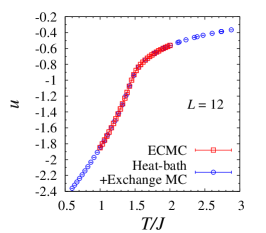
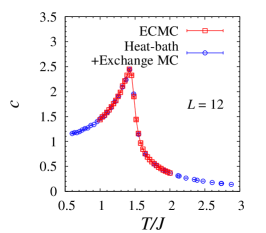
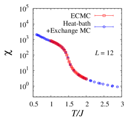
Figure 1: (Color online) Temperature dependence of the energy density $e=E/N$, the specific heat $c$ and the magnetic susceptibility $\chi$ of the three-dimensional Heisenberg model with $L=12$. A chain length $\ell=N\pi/10$ is used.

Applied to the Heisenberg model, the ECMC augments the physical space of spin configurations by a lifting variable $(k,\boldsymbol{v})$ which specifies the considered infinitesimal counterclockwise rotation of spin $k$ about the axis $\boldsymbol{v}$. By virtue of the factorized Metropolis filter, this physical move can only be rejected by a single neighboring spin, $l$, and the lifting variable will then be moved as $(k,\boldsymbol{v})\to(l,\boldsymbol{v})$, keeping the sense of rotation, but passing it on to the spin responsible for the rejection. In the augmented space, the rejections are thus supplanted by events, namely the lifting moves for arrested physical states. The ECMC, for a given axis $\boldsymbol{v}$, breaks detailed balance, yet satisfies global balance, as the probability flow into each lifted configuration equals the flow out of it, to first order in the time increment $\mathrm{d}t$. For the $XY$ model of planar rotators, $\boldsymbol{v}$ is uniquely defined as the axis perpendicular to the sense of rotation. For this reason, the ECMC around this axis is irreducible, and the chain length $\ell$ in this model is best taken equal to the simulation time Michel_2015 . For the Heisenberg model, spin rotations must be about at least two axes, in order to reach the entire configuration space. The resampling of the rotation axis is performed after the cumulative rotation angles about the previous axis reaches the chain length $\ell$. All configurations of the chain sample the equilibrium distribution and any uniform subset of them yield valid observable averages. Observables may be integrated during the continuous evolution or e.g. retrieved at regular intervals independent of the lifting events.

For a fixed rotation axis $\boldsymbol{v}$, the ECMC algorithm for the Heisenberg model reduces to the one of the $XY$ model: With $(\phi_{\boldsymbol{v},k},\theta_{\boldsymbol{v},k})$ the spherical coordinates of a spin $k$ in a system where the $z$-axis is aligned with $\boldsymbol{v}$, the pair energy $E_{kl}$ between spins $k$ and $l$ is

$$E_{kl} =-J^{\prime}\cos(\phi_{\boldsymbol{v},k}-\phi_{\boldsymbol{v},l})+K$$ (3)

with

$$J^{\prime} =J\sin\theta_{\boldsymbol{v},k}\sin\theta_{\boldsymbol{v},l},$$

$$K =-J\cos\theta_{\boldsymbol{v},k}\cos\theta_{\boldsymbol{v},l}.$$

Both $J^{\prime}$ and $K$ depend only on the polar angles $\theta_{\boldsymbol{v}}$ and remain unchanged along the event chain. The azimuthal-angle dependence in Eq. (3) is $\propto\cos(\phi_{\boldsymbol{v},k}-\phi_{\boldsymbol{v},l})$, as in the $XY$ model.

The azimuthal angle $\phi_{\boldsymbol{v},k}$ increases for each ECMC chain from its initial value $\phi_{0}$ until one of its neighbors, $l$, triggers a lifting $(k,\boldsymbol{v})\to(l,\boldsymbol{v})$ at $\phi_{\boldsymbol{v},k}=\phi_{l,\text{event}}$. The latter is sampled with a single random number in the event-driven approach Peters_2012 ; Michel_2014 . Precisely, $\phi_{l,\text{event}}$ is given by the sampling of the positive pair energy increase:

$$\Delta E_{l}=-\left[\log\ \text{ran}(0,1)\right]/\beta=\\ -J^{\prime}\int^{\phi_{l,\text{event}}}_{\phi_{0}}\max\left(0,\frac{\mathrm{d}\cos(\phi_{\boldsymbol{v},k}-\phi_{\boldsymbol{v},l})}{\mathrm{d}\phi_{\boldsymbol{v},k}}\right)\mathrm{d}\phi_{\boldsymbol{v},k},$$ (4)

where $\text{ran}(0,1)$ is a uniform random number between $0$ and $1$. To solve Eq. (4) for $\phi_{l,\text{event}}$, one first slices off any full rotations (these $n$ rotations by $2\pi$ yield an energy increase of $2nJ^{\prime}$), leaving a value $\Delta E_{l}^{f}$,

$$E^{*}_{\text{init}}+\Delta E_{l}^{f}=-J^{\prime}\cos(\phi_{l,\text{event}}-\phi_{\boldsymbol{v},l}-2n\pi),$$ (5)

where

$$E^{*}_{\text{init}}=\begin{cases}E_{kl}&\text{if initial pair energy change $>0$}\\ -J^{\prime}&\text{otherwise}.\end{cases}$$

The true lifting event corresponds to the earliest of the independent event times sampled for all the neighbors of the spin $k$. In ECMC, Monte Carlo time is continuous and proportional to the total displacement of the spins. We have checked the correctness of the ECMC, and obtained perfect agreement for the mean energy, the specific heat and the susceptibility with the heat-bath algorithm Miyatake_1986 ; Olive_1986 modified with the exchange Monte Carlo method (or “parallel tempering”) Hukushima_1996 (see Fig. 1).

III Dynamical scaling exponent

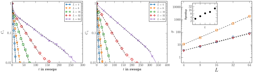
Figure 2: Autocorrelation functions and time constants of ECMC for the three-dimensional Heisenberg model at its critical point $\beta=0.693$. Left: Energy density autocorrelation function $C_{e}$ for for system sizes $4^{3}$, $8^{3}$, …, $64^{3}$. Center: Susceptibility autocorrelation function $C_{\chi}$ for ECMC for the three-dimensional Heisenberg system sizes $4^{3}$, $8^{3}$, …, $64^{3}$. Right: Scaling of the autocorrelation time $\tau_{\chi}$ (resp. $\tau_{e}$) of the susceptibility $\chi$ (resp. energy density $e$) with system size $L$ for ECMC (blue circles) (resp. (red triangles)) and of the autocorrelation time of the susceptibility for LMC (yellow squares). Error bars are smaller than the markers size. Right Inset: Speedup for the susceptibility $\chi$ in comparison to LMC for system sizes $4^{3}$, $8^{3}$, …, $64^{3}$.

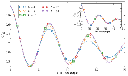
Figure 3: (Color online) Autocorrelation function of magnetization $C_{M}(t)$ at the critical temperature for various system sizes. The inset shows the spin autocorrelation function of a trivial algorithm that only performs global rotations in spin space along the two axes.

At the critical temperature $T_{\mathrm{c}}$, the correlation length $\xi$ of a model undergoing a second-order phase transition equals the system size $L$ and the autocorrelation time of slow variables $\tau$ diverges as $\tau\sim L^{z}$, where $z$ is the dynamical critical exponent. We measure time in sweeps: One ECMC sweep corresponds, in average, to $N$ lifting events and one LMC sweep to $N$ attempted moves. Time autocorrelation functions are defined by

$$C_{O}(t) = \frac{\left\langle O(t^{\prime}+t)O(t^{\prime})\right\rangle-\left\langle O(t^{\prime})\right\rangle^{2}}{\left\langle O^{2}(t^{\prime})\right\rangle-\left\langle O(t^{\prime})\right\rangle^{2}},$$ (6)

where the brackets $\langle\cdots\rangle$ indicate the thermal average and $t^{\prime}$ is set sufficiently large for equilibration. The dynamical critical exponent of LMC for the three-dimensional Heisenberg model was estimated from the autocorrelation function of the magnetization $\boldsymbol{M}$ as $z=1.96(6)$Peczak_1993 . The over-relaxation algorithm Creutz_1987 ; Brown_1987 seems to give $z\simeq 1.10$ Peczak_1993 which was obtained from the autocorrelation function of the magnetization, and the Wolff algorithm is believed to yield a value close to zero: $z\gtrsim 0$, a value obtained from the susceptibility autocorrelation function Holm_1993 .

To evaluate the correlation time and the dynamical critical exponent for the ECMC, one must pay attention to the irreversible nature of the underlying Markov chain. During one event chain, spins all rotate in the same sense, and the system undergoes global rotations with taking into account the thermal fluctuation. This results in fast oscillations of the magnetization $\boldsymbol{M}$ and a quick decay of its autocorrelation function that is insensitive to the system size (see Fig. 3), and even to the temperature. However, this effect is also visible for a trivial algorithm, which simply performs global rotations (see the inset of Fig. 3). The trivial algorithm satisfies global balance, but its correlation time is infinite, as it does not relax the energy. A similar effect appears in the ECMC for particle systems Bernard_2009 , that likewise is not characterized by the mean net displacement of particles. To characterize the speed of the ECMC, we consider the energy density and the susceptibility that we conjecture to be slow variables at the critical temperature. Both $\chi$ and $e$ are insensitive to global rotations and do not oscillate.

As shown in Fig. 2, the autocorrelation functions both of the energy density and of the susceptibility are well approximated as a single exponential decay

$$C_{\chi}(t)=\exp(-t/\tau)$$ (7)

on essentially the same timescales. Furthermore, the finite-size behavior of the autocorrelation times indicates $z\simeq 1$ dynamical scaling. This $z$ value is significantly less than for the LMC and very similar to the one obtained for over-relaxation methods, although the $z\simeq 0$ value of the cluster algorithm is not reached.

IV Discussion and summary

The earliest application of lifting Diaconis_2000 , the motion of a particle on a one-dimensional $N$-site lattice with periodic boundary conditions, already featured the decrease of the dynamical scaling exponent from $z=2$ to $z=1$ (the reduction of the mixing time from $\propto N^{2}$ to $\propto N$). To reach such reductions, the Markov chain must be irreversible. It was pointed out that the “square-root” decrease of the critical exponent was the optimal improvement Chen_1999 . The concepts of factorized Metropolis filters and of infinitesimal moves bring irreversible lifting algorithms to general $N$-body systems, although only finite speed-ups were realized so far in the $N\to\infty$ limit. The three-dimensional Heisenberg model seems to be a first such ECMC application with a lowered critical dynamical exponent. Our observation relies on the hypotheses that the energy and the susceptibility are indeed “slow” variables, and that the observed decay of the autocorrelation function continues for larger times. However, in Fig. 2, a crossover from $z=1$ back to $z=2$ as it was observed in the $XY$-model after $\sim 5$ sweeps Michel_2015 appears unlikely to arise after hundreds of sweeps. The dynamical critical exponent $z\approx 1$ represents a maximal improvement with respect to the $z\approx 2$ of LMC, supposing again that the theorems of ref. Chen_1999 apply to infinitesimal Markov chains.

In summary, we have successfully applied ECMC to the Heisenberg model in three dimensions. ECMC shows considerable promise for spin models, and the numerical data presented in this paper allow us to formulate the exciting conjecture that the dynamical critical exponent for the Heisenberg model is $z\simeq 1$. ECMC is also applicable to frustrated magnets and spin glasses, which involve antiferromagnetic interactions and/or quenched disorder. Our preliminary study indicates that the ECMC algorithm is also useful for a Heisenberg spin glass model. ECMC can be easily combined with other algorithms such as the exchange Monte Carlo method and the over-relaxation algorithm in the usual manner. This may allow to investigate the three-dimensional Heisenberg spin glass model in the low-temperature region. Large-scale simulations in this direction are currently in progress. It would be very interesting to understand why ECMC is so much more successful in the Heisenberg model than both in hard and soft disks and in the $XY$ model.

References

- (1) N. Metropolis, A. W. Rosenbluth, M. N. Rosenbluth, A. H. Teller and E. Teller, J. Chem. Phys. 21, 1087 (1953).
- (2) R. H. Swendsen and J. S. Wang, Phys. Rev. Lett. 58, 86 (1987).
- (3) U. Wolff, Phys. Rev. Lett. 62, 361 (1989).
- (4) B. A. Berg and T. Neuhaus, Phys. Rev. Lett. 68, 9 (1992).
- (5) K. Hukushima and K. Nemoto, J. Phys. Soc. Jpn. 65 1604 (1996).
- (6) H. Suwa and S. Todo, Phys. Rev. Lett. 105, 120603 (2010).
- (7) K. S. Turitsyn, M. Chertkov and M. Vucelja, Physica D 240, 410 (2011).
- (8) H. C. M. Fernandes and M. Weigel, Comput. Phys. Commun. 182, 1856, (2011).
- (9) E. P. Bernard, W. Krauth, and D. B. Wilson, Phys. Rev. E 80, 056704 (2009).
- (10) E. P. Bernard and W. Krauth, Phys. Rev. Lett. 107, 155704 (2011).
- (11) M. Isobe and W. Krauth, J. Chem. Phys 143, 084509 (2015).
- (12) M. Michel, S. C. Kapfer, and W. Krauth, J. Chem. Phys. 140, 054116 (2014).
- (13) E. A. J. F. Peters and G. de With, Phys. Rev. E 85, 026703 (2012).
- (14) S. C. Kapfer and W. Krauth, Phys. Rev. Lett. 114, 035702 (2015).
- (15) M. Michel, J. Mayer, and W. Krauth, arXiv:1508.06541 (2015).
- (16) P. Diaconis, S. Holmes, and R. M. Neal, Annals of Applied Probability 10, 726 (2000).
- (17) F. Chen, L. Lovasz, and I. Pak, Proc. 17th Annual ACM Symposium on Theory of Computing, 275 (1999).
- (18) K. Chen, A. M. Ferrenberg and D. P. Landau, Phys. Rev. B 48, 3249 (1993).
- (19) Y. Miyatake, M. Yamamoto, J. J. Kim, M. Toyonaga and O. Nagai, J. Phys. C: Solid State Phys. 19, 2539 (1986).
- (20) J. A. Olive, A. P. Young and D. Sherrington, Phys. Rev. B, 34 6341 (1986).
- (21) P. Peczak and D. P. Landau, Phys. Rev. B 47, 14260 (1993).
- (22) M. Creutz, Phys. Rev. D 36, 515 (1987).
- (23) F. R. Brown and T. J. Woch, Phys. Rev. Lett. 58, 2394 (1987).
- (24) C. Holm and W. Janke, Phys. Rev. B 48, 936 (1993).