Regular and Chaotic Classical and Quantum Dynamics in Multi-Well Potentials

Chapter 1 Introduction

Currently we can consider as a rigorously established fact the existence of dynamical systems with a small number of degrees of freedom ($N\geq 2$ — in autonomous case, $N\geq 1$ — for non-autonomous systems) for which under certain conditions classical motion cannot be distinguished from random motion [1, 2, 3, 5]. Typical features of these systems are nonlinearity and the absence of any external source of randomness. Thus, using such synonyms for the term ”random” as ”chaotic”, ”stochastic”, ”irregular”, we can state that there are nonlinear deterministic systems for which these notions express adequately internal fundamental properties that comprise important and interesting subjects for investigation. For the last 30-40 years examples of chaotic motion have been detected in every field of natural science, and their number continues to grow.

The mechanism which is responsible for the existence of chaotic regimes in purely deterministic systems is based on local instability. It leads to exponential divergence of initially close trajectories

$$d(t)=d(0)e^{ht}$$

where $d$ is the distance between two points in phase space that belong to different trajectories. It could be shown [6] that local instability leads to mixing i.e. splitting of time correlations

$$\lim_{t\rightarrow\infty}R(f,\varphi)\sim e^{-h_{c}t}$$

for arbitrary functions in phase space $f(z),\varphi(z)\left(z(t)=[q(t),p(t)]\right)$. A principally new result that was established by N.Krylov [6] consisted in the understanding that the averaged increment of local instability $\langle h\rangle$ determines the time of correlations splitting

$$h_{c}=\langle h\rangle.$$

This equation exactly establishes the connection between the dynamics of the system and its statistical properties. In other words, we must understand stochasticity as a rise of statistical features in the system as a result of local instability.

Local instability of trajectories makes the problem of assignment of initial conditions in classical mechanics as fundamental as the uncertainty principle makes the problem of measurement in quantum mechanics. From the traditional viewpoint finite precision is limited by the imperfection of the measuring instrument. But the new viewpoint is different: we could not record the result of the measurement with infinite precision even if the ideal measuring instrument were constructed — there is not enough energy, time and paper. Uncertainty of measurement could not be completely eliminated even as a theoretical idea because inaccuracy in the data-line of a purely deterministic system is not produced by external randomness or noise but is connected with the finite precision of initial conditions assignment instead. In particular, at the beginning of the last century Poincaré showed [7] that for some astronomical systems a tiny imprecision in the initial conditions would grow in time at an enormous rate. Thus two nearly-indistinguishable sets of initial conditions for the same system would result in two vastly different final predictions. In the presence of local instability this inaccuracy leads to very peculiar behavior of deterministic systems. For most physicists ”dynamical instability” and ”chaos” became convertible terms.

Fundamental progress in the understanding of classical nonlinear dynamics caused numerous attempts to integrate the concept of stochasticity into quantum mechanics. The core of the problem lies in the fact that energy spectrum of every quantum system is discrete and thus motion is quasiperiodic if the system demonstrates finite motion. On the other hand, the correspondence principle demands the possibility of transition to classical mechanics which demonstrates not only regular regimes but chaotic too. Several important results that clarify this contradiction were established. However, long before complete solution of the problem there has been interest in its reduced variant – the search for peculiarities in the behavior of quantum systems which have chaotic classical analogues. These peculiarities are called Quantum manifestations of classical stochasticity (QMCS).

Many decades would pass before dynamical chaos ideology was realized by the science community as a whole. According to the old ideology:

• Chaos is an attribute of a compound system.

• In any compound system it is possible to find out the elements of chaos.

• Useful information is contained in those few places in which chaos is absent.

• Physicists must look for non-chaos.

The new ideology changed the situation principally:

• Chaos is universal inalienable property of simple deterministic systems.

• Chaotic dynamics is the most general way of evolution of an arbitrary nonlinear system

• New interesting information is contained exactly in those branches of natural sciences where chaos is present.

• Chaos is the major object of study.

• The physicist must look for chaos! [8].

The basis of the present report is the new chaos ideology. In the context of this approach a general investigation of arbitrary nonlinear dynamical system involves the following steps:

1. Investigation of the classical phase space, detection of chaotic regimes by numerical and analytical analysis of the classical equations of motion.

2. Analytical estimation of the critical energy for the onset of global stochasticity.

3. Test for QMCS in the energy spectra, eigenfunctions and wave packet dynamics.

4. Consideration of the interrelationship between stochastic dynamics and concrete physical effects.

The basic subject of the current report is to realize the outlined program for two-dimensional Hamiltonian systems with potential energy surface which has several local minima, i.e. multi-well potentials.

Despite the huge number of papers concerning chaotic dynamics, Hamiltonian systems with multi-well potentials have been somewhat neglected. Nevertheless the Hamiltonian system with multi-well potential energy surface (PES) represents a realistic model, describing the dynamics of transition between different equilibrium states, including such important cases as chemical and nuclear reactions, nuclear fission, phase transitions, string landscape and many others. Being substantially nonlinear, such systems represent a potentially important object, both for the study of classic chaos and QMCS.

Chapter 2 Specifics of Classical Dynamics in Multi-Well Potentials — Mixed State

Let us consider the characteristics of classical finite motion in multi-well potentials. They are more complicated than in single-well potentials and allow the existence of several critical energies even for a fixed set of potential parameters. This fact results in the so-called mixed state in such potentials [9]: at the same energy there are different dynamical regimes in different wells, either regular or chaotic. It is important to note that mixed state is a general feature of the Hamiltonians with nontrivial PES. For the first example, let us demonstrate the existence of mixed state for nuclear quadrupole oscillations Hamiltonian [10]. It can be shown that, using only transformation properties of the interaction, the deformation potential of surface quadrupole oscillations of nuclei takes the form [11]:

$$U(a_{0},a_{2})=\sum\limits_{m,n}C_{mn}(a_{0}^{2}+2a_{2}^{2})^{m}a_{0}^{n}(6a_{2}^{2}-a_{0}^{2})^{n}$$ (2.1)

where $a_{0}$ and $a_{2}$ are internal coordinates of the nuclear surface during the quadrupole oscillations:

$$R(\theta,\varphi)=R_{0}\{1+a_{0}Y_{2,0}(\theta,\varphi)+a_{2}[Y_{2,2}(\theta,\varphi)+Y_{2,-2}(\theta,\varphi)]\}$$

Constants $C_{mn}$ can be considered as phenomenological parameters. Restricting to the terms of the fourth degree in the deformation and assuming the equality of mass parameters for two independent directions, we get $C_{3v}$-symmetric Hamiltonian:

$$H=\frac{p_{x}^{2}+p_{y}^{2}}{2m}+U_{QO}(x,y;a,b,c)$$ (2.2)

where

$$\begin{array}[]{c}U_{QO}(x,y;a,b,c)=\frac{a}{2}(x^{2}+y^{2})+b\left(xy^{2}-\frac{x^{3}}{3}\right)+c(x^{2}+y^{2})^{2}\\ x=a_{0},\ y=\sqrt{2}a_{2},\ a=2C_{10},\ b=3C_{01},\ c=C_{20}\end{array}$$

This potential is a generalization of the well-known Hénon-Heiles potential [12], which became a traditional object for examination of new ideas and methods in investigations of stochasticity in Hamiltonian systems. It is essential that, in contrast to Hénon -Heiles potential, motion in (2.2) is finite for all energies, assuring the existence of stationary states in the quantum case. Hamiltonian (2.2) and corresponding equations of motion depend only on parameter $W=b^{2}/(ac)$, the unique dimensionless quantity we can build from parameters $a,b,c$. The same parameter determines the geometry of PES

$$U_{QO}(x,y;W)=\frac{1}{2W}(x^{2}+y^{2})+xy^{2}-\frac{x^{3}}{3}+(x^{2}+y^{2})^{2}$$ (2.3)

Interval $0<W<16$ includes potentials with a single extremum — minimum in the origin that corresponds to the spherically symmetric shape of the nucleus. In the interval $W>16$ PES of $U_{QO}$ contains seven extrema: four minima (one central, placed in the origin, and three peripheral, which correspond to deformed states of nuclei) and three saddles, which separate the peripheral minima from the central one (Fig.2.1).

Figure 2.1: The level lines of the PES (2.3) for different structurally stable domains.

Numerical calculations of equations of motion in the region $0<W<16$ (region of single-well potentials) indicate regularity–chaos–regularity (R-C-R) transition: gradual transition from regular to chaotic motion when energy increases and restoration of regular motion for high energies (fig.2.2). In the next section we will discuss in details possible stochastization scenarios and methods of critical energy calculation.

Figure 2.2: The R-C-R transition in the quadrupole oscillations potential (2.3).

In the region $W>16$ (multi-well potentials) we confront with a substantially more complicated situation. In Figure 2.3 there are presented Poincaré surfaces of section (PSS) for different energies. They demonstrate evolution of dynamics in central and peripheral minima of QO potential $U_{QO}$ (with $W=18$, when depths of central and peripheral minima are equal). At low energies motion is clearly quasi-periodic for both minima. Let us pay attention to the difference in topology of PSS. In the central minimum, PSS structure is complicated and has fixed points of different types, while in peripheral minima PSS has trivial structure with only one elliptical fixed point.

When energy increases, gradual transition to chaos is observed, but changes in character of motion are totally different in different minima. In the central minimum already at energy equal to a half of the saddle energy $E_{S}$, a sizeable part of the trajectories is chaotic, and at the saddle energy there are almost no regular trajectories at all. At the same conditions, in the peripheral minimum motion remains quasiperiodic. Furthermore, even at energies higher than the saddle energy there is a substantial part of the phase space occupied by quasiperiodic motion. In other words dynamics above the barrier has some kind of ”memory”: the structure of phase space at energies greater than the saddle one is determined by the character of the motion in the local minima.

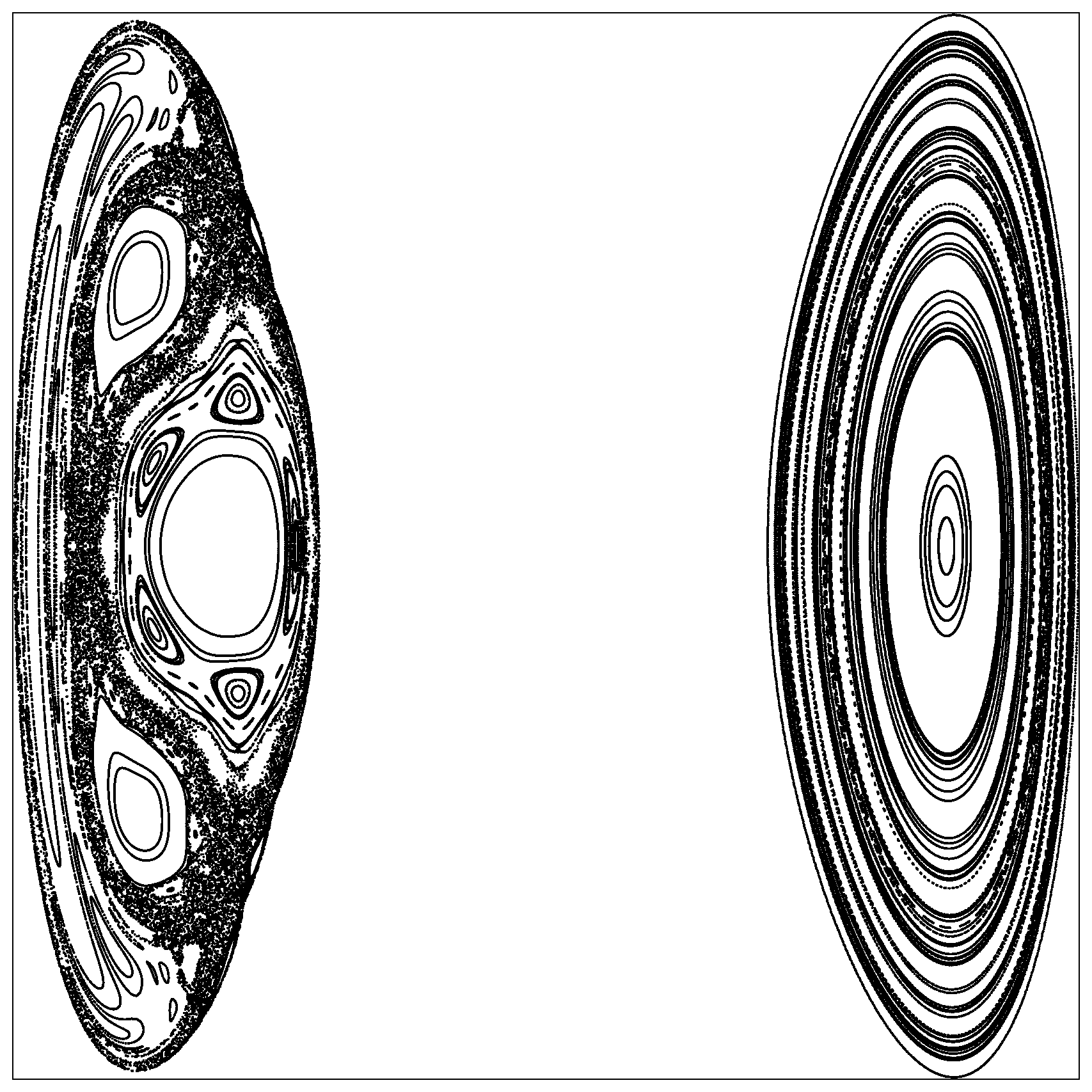
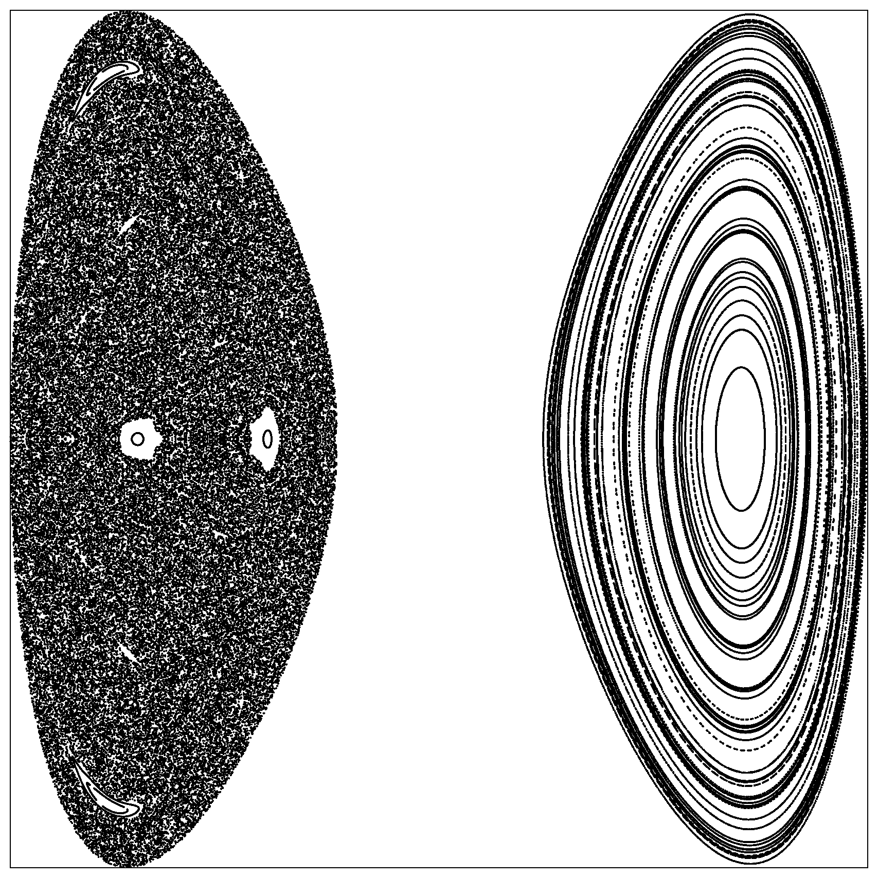
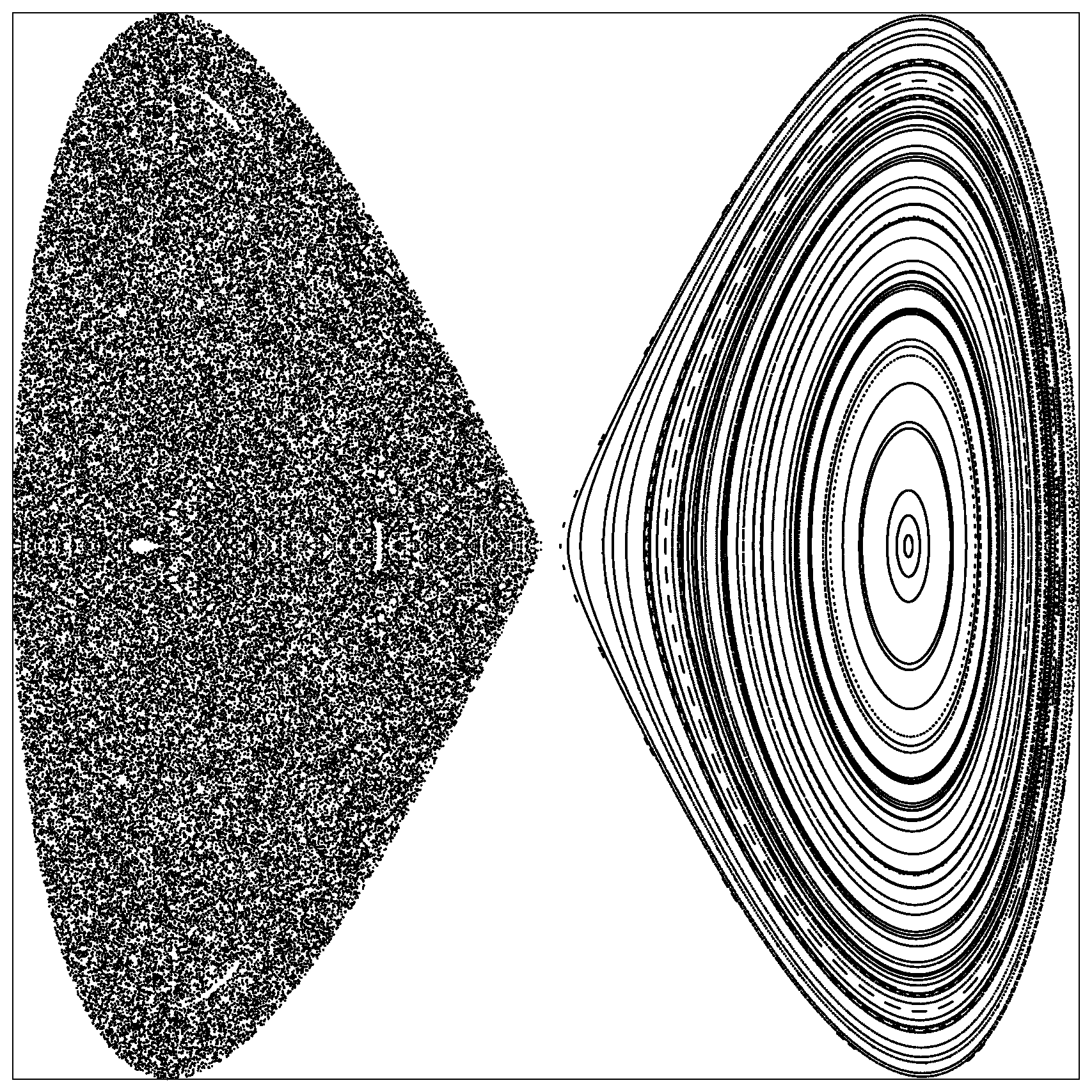
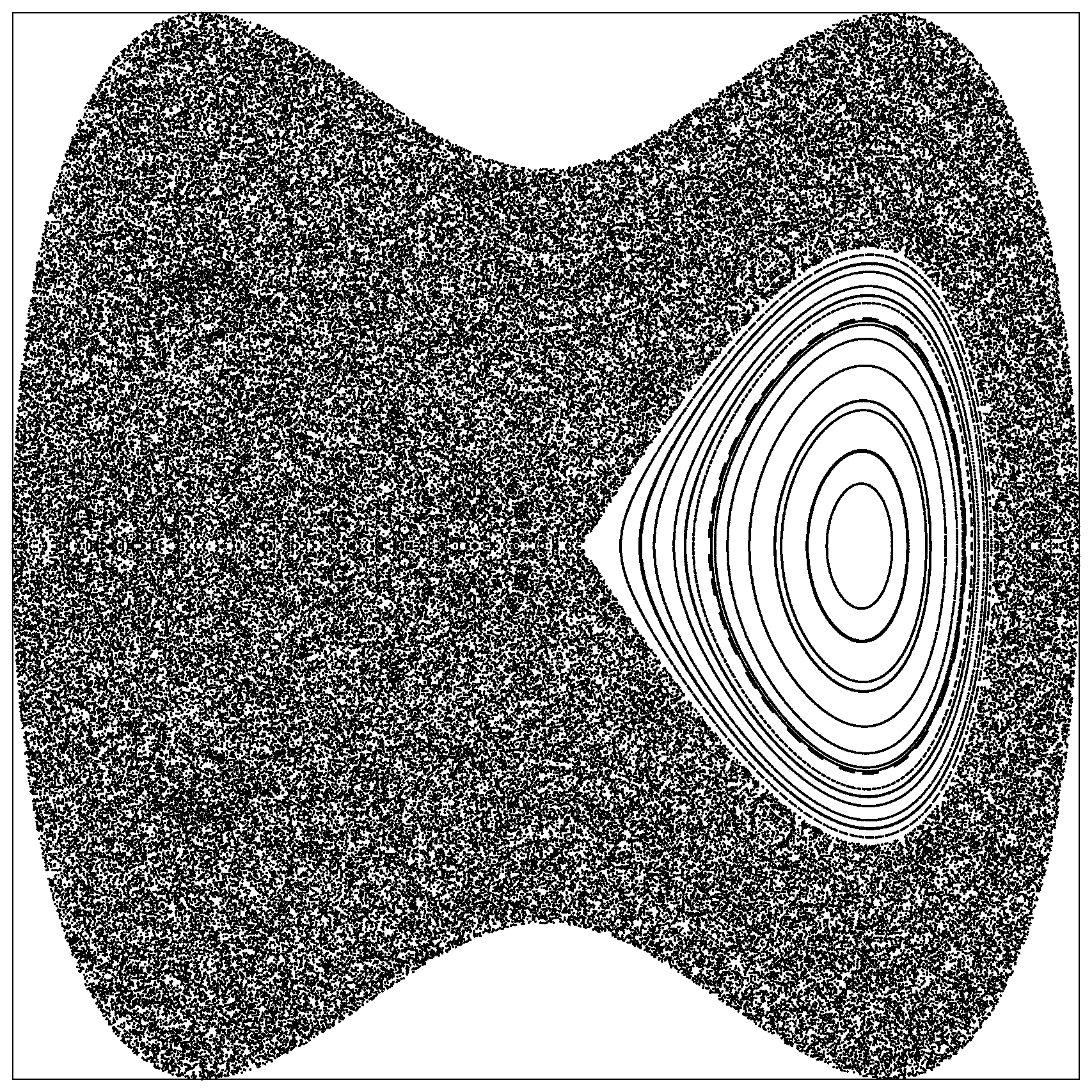
Figure 2.3: PSS for motion in the potential $U_{QO}$ (2.3) with $W=18$ at different energies: $E/E_{S}=\{0.5,0.8,1,2\}$.

Thus, in the energy region $E_{S}/2<E<E_{S}$, classical dynamics is clearly chaotic in the central minimum and remains regular in peripheral minima. This type of dynamics, when chaoticity measured at fixed energy significantly differs in different local minima, represents the common case situation in multi-well potentials and is called the mixed state.

As an example of the concrete realization of the (2.1) potential, let us consider deformational potential, that describes quadrupole oscillations of Krypton isotopes. Seiwert, Ramayya and Maruhn [13] restored the parameters of the deformation potential of the quadrupole oscillations, including the sixth degree terms in deformation for isotopes $Kr^{74,76,78,80}$

$$\begin{array}[]{c}U_{QO}(x,y;a,b,c)=\frac{a}{2}(x^{2}+y^{2})+b\left(xy^{2}-\frac{x^{3}}{3}\right)+c(x^{2}+y^{2})^{2}+\\ +b\left(xy^{2}-\frac{x^{3}}{3}\right)(x^{2}+y^{2})+e\left(xy^{2}-\frac{x^{3}}{3}\right)^{2}+f(x^{2}+y^{2})^{3}.\end{array}$$

The big experimental values of energy of the first $2^{+}$-states for nuclei $Kr^{74,76}$ indicate a spherical shape of nucleus surface, while the probabilities of the electromagnetic transitions $2^{+}\rightarrow 2^{0}$ and very low energies of first rotational states imply the possibility of superdeformation. The nonlinear effects, which are connected with the geometry of PES must be exhibited in the superdeformed nuclei at relatively low energies of excitation. The PES of Krypton isotopes are presented in Fig.2.4.

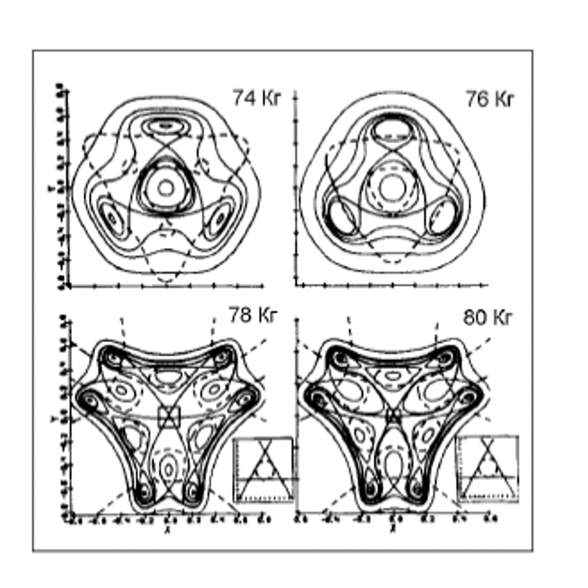
Figure 2.4: The PES of Krypton isotopes.

As can be seen, inclusion of higher terms of expansion leads to considerable complication of the PES geometry: for all considered Krypton isotopes we run into potentials with PES of complicated topology with many local minima. It s clear that, for all potential surfaces, $C_{3v}$-symmetry is preserved.

The mixed state, which was shown above for the potential of quadrupole oscillations, is the representative state for a wide class of two-dimensional potentials with few local minima. According to the catastrophe theory [14], a rather wide class of polynomial potentials with several local minima is covered by the germs of the lowest umbilical catastrophes, of type $D_{5}$, $D_{4}^{-}$, $D_{7}$, subjected to certain perturbations. Let us note that the Hénon-Heiles potential coincides with the elliptic umbilic $D_{4}^{-}$. Fig.2.5 represents level lines and Poincaré sections at different energies for multi-well potentials from a family of umbilical catastrophes $D_{5}$ and $D_{7}$:

$$U_{D_{5}}=2y^{2}-x^{2}+xy^{2}+\frac{1}{4}x^{4}+1$$ (2.4)

$$U_{D_{7}}=\sqrt{2}y^{2}+\frac{3}{8}x^{2}+xy^{2}-\frac{1}{2}x^{4}+\frac{1}{6}x^{6}$$

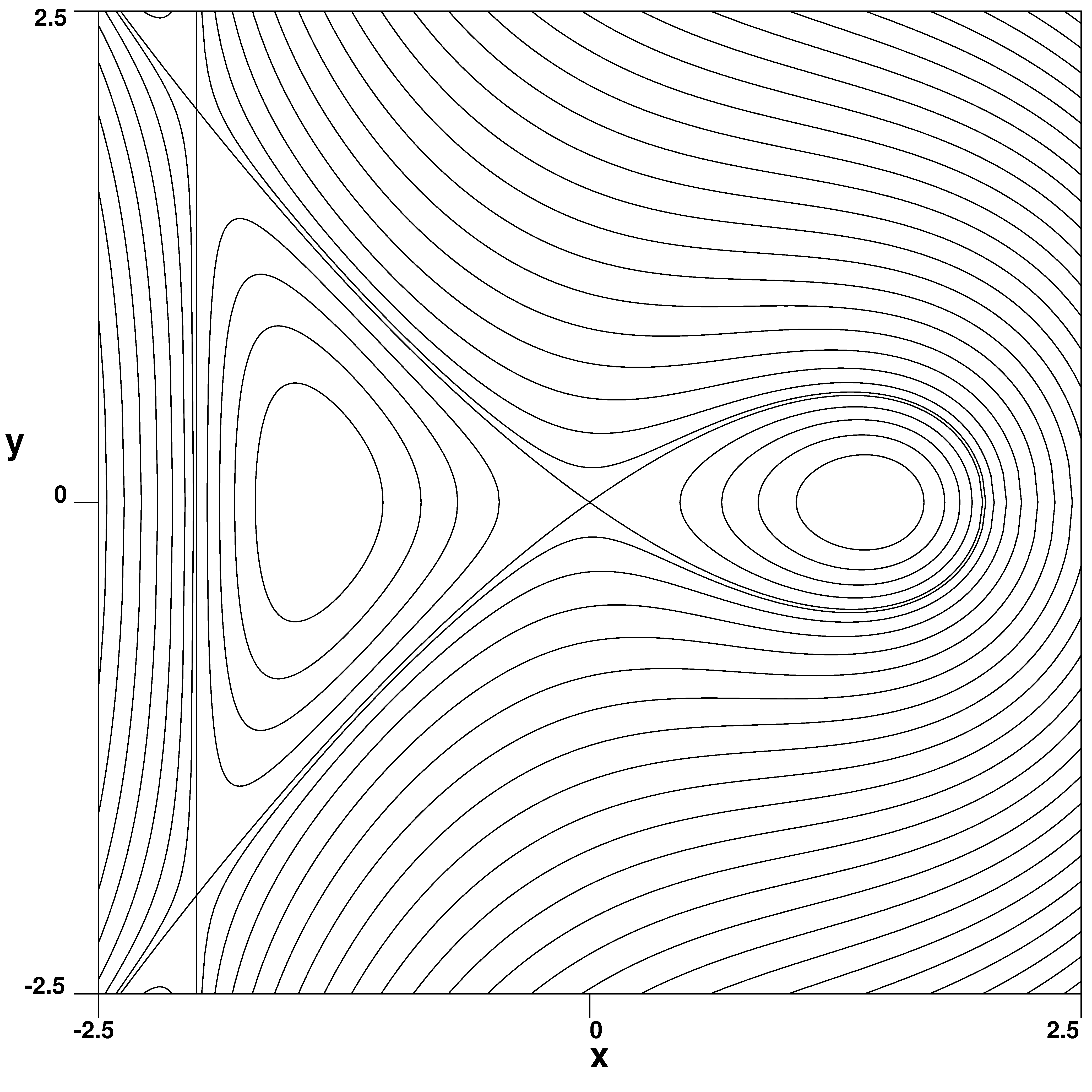
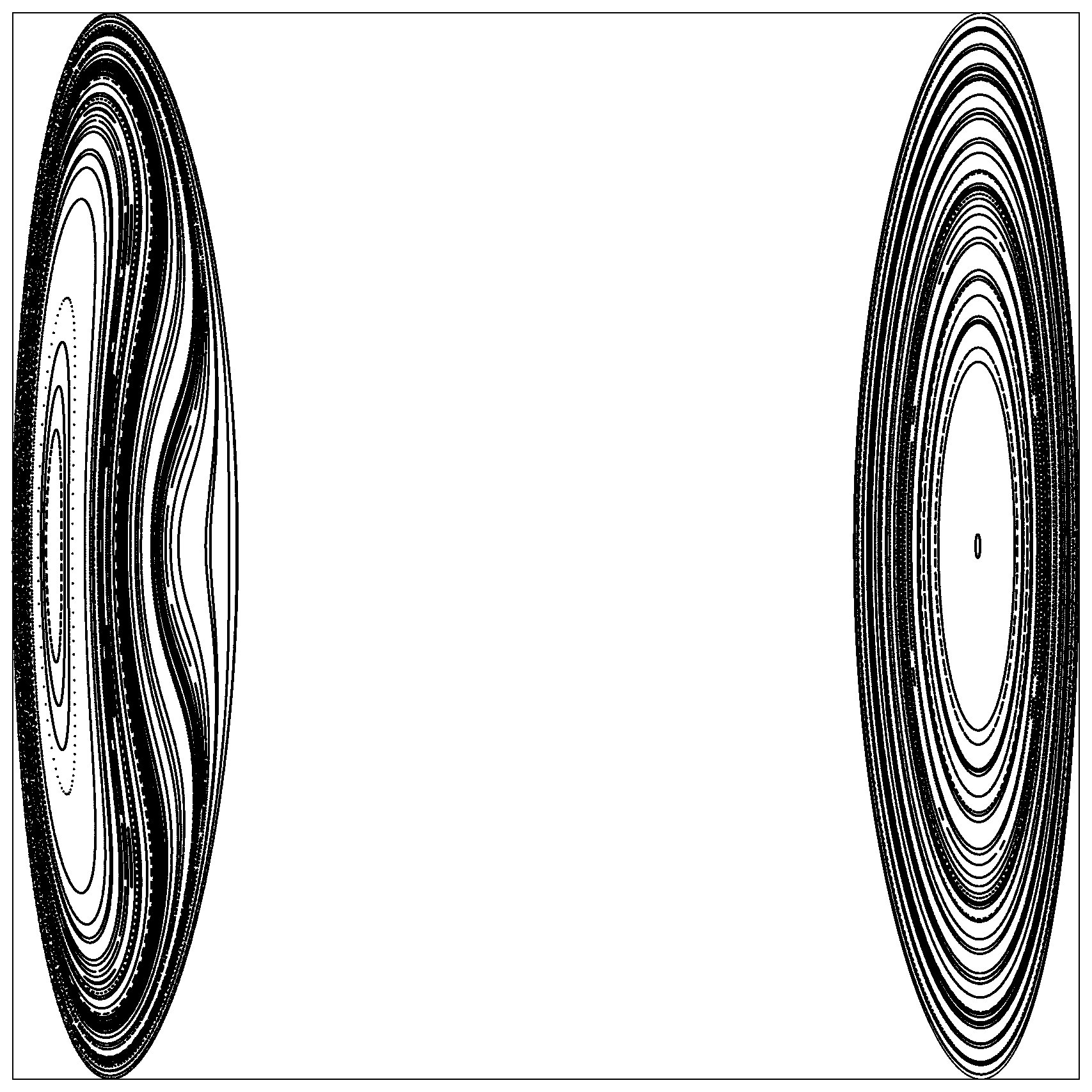
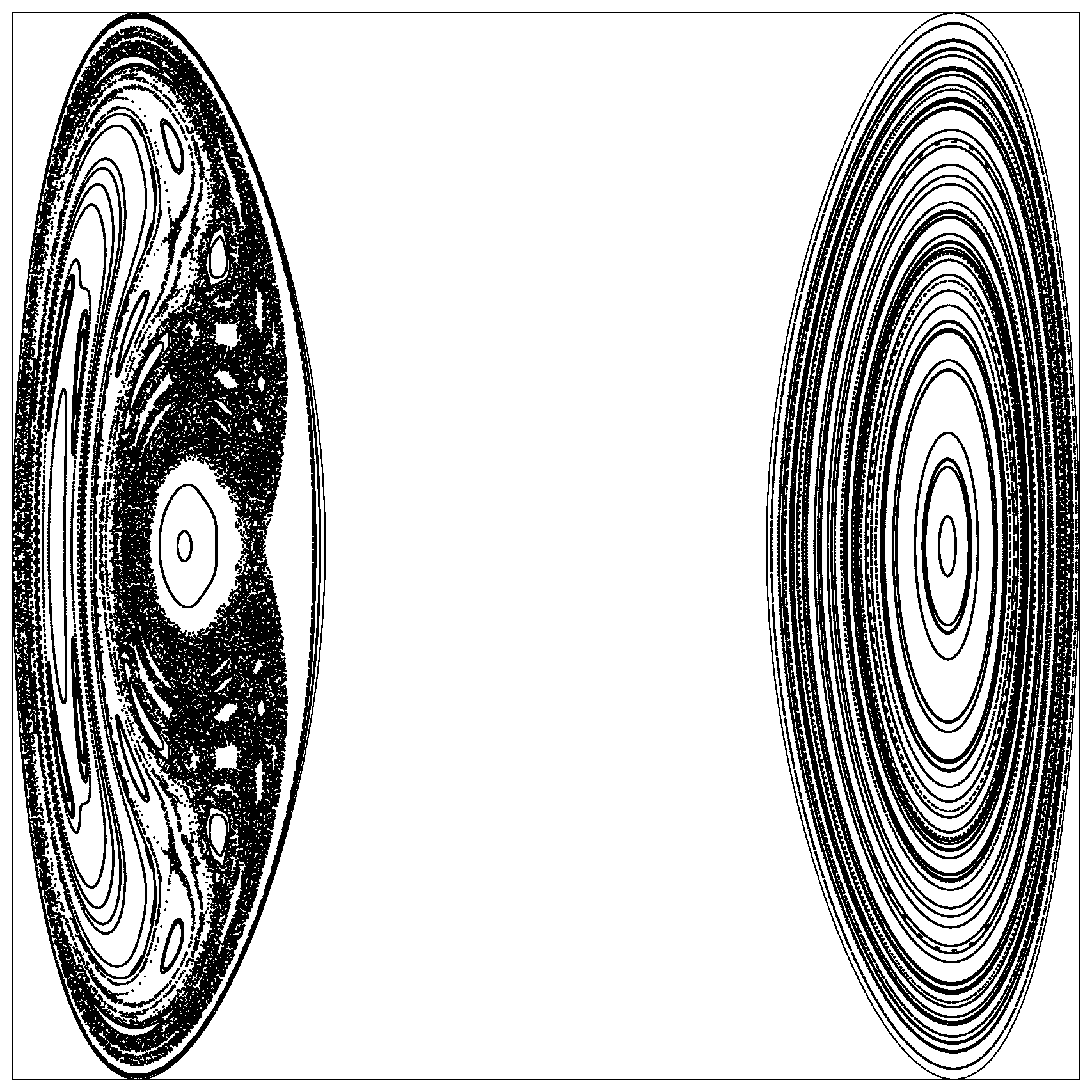
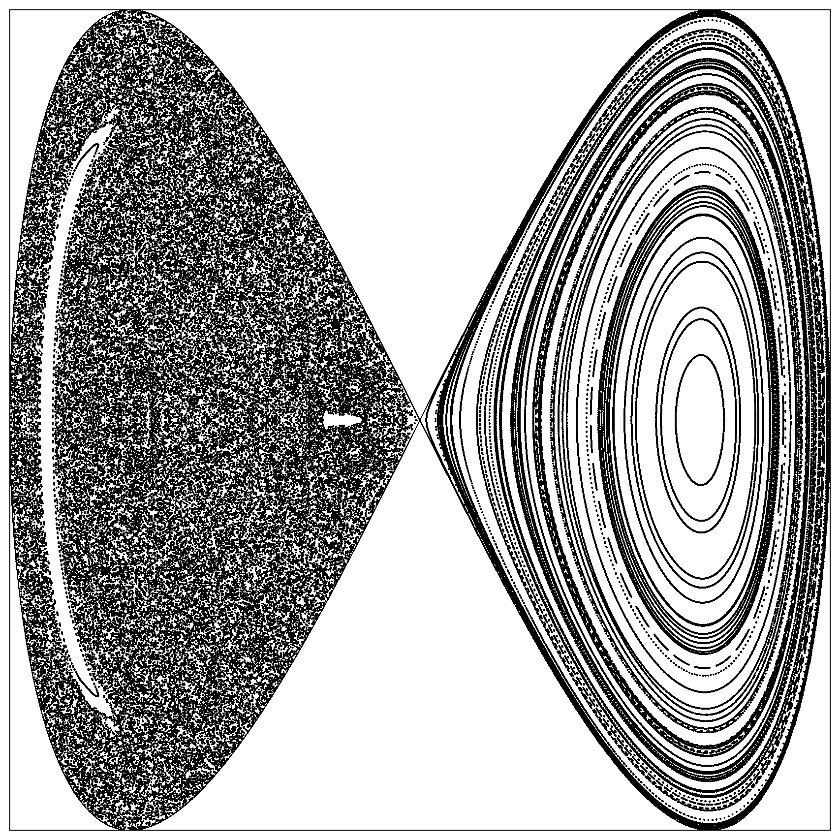
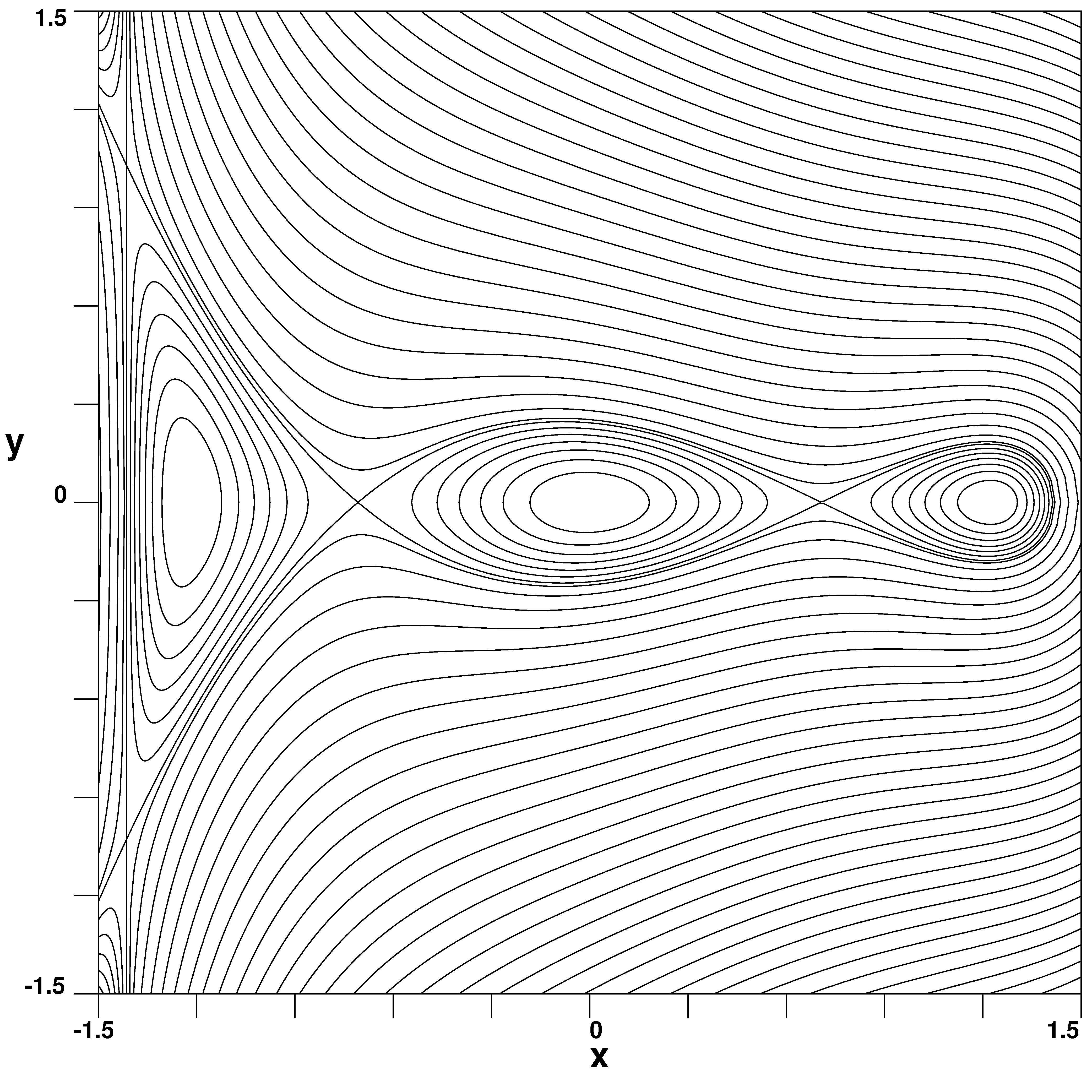
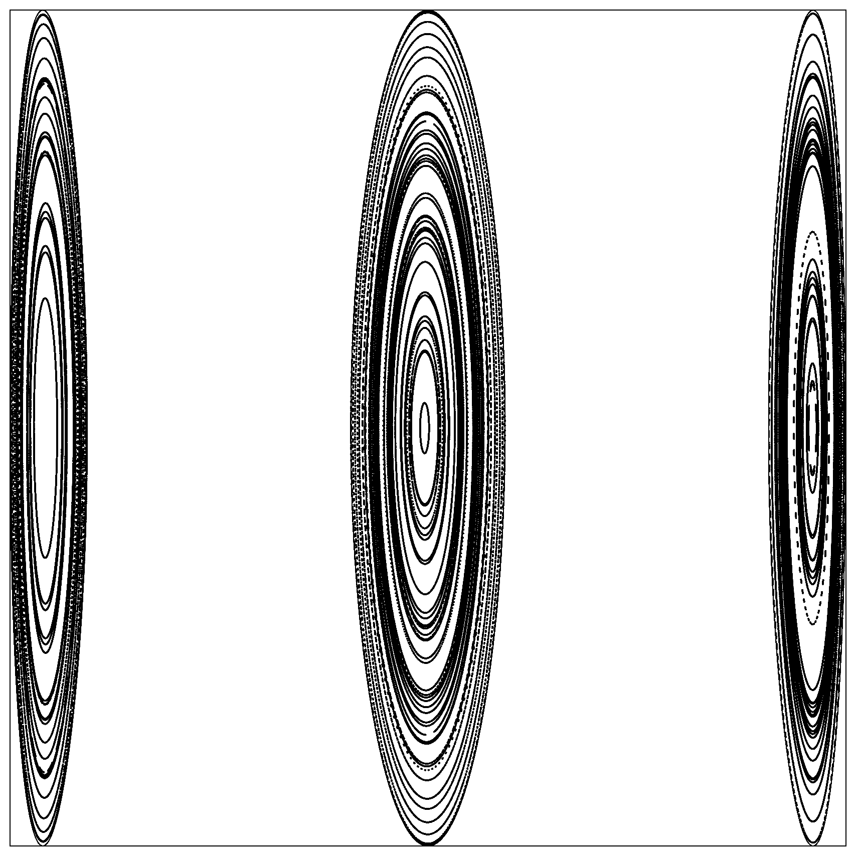
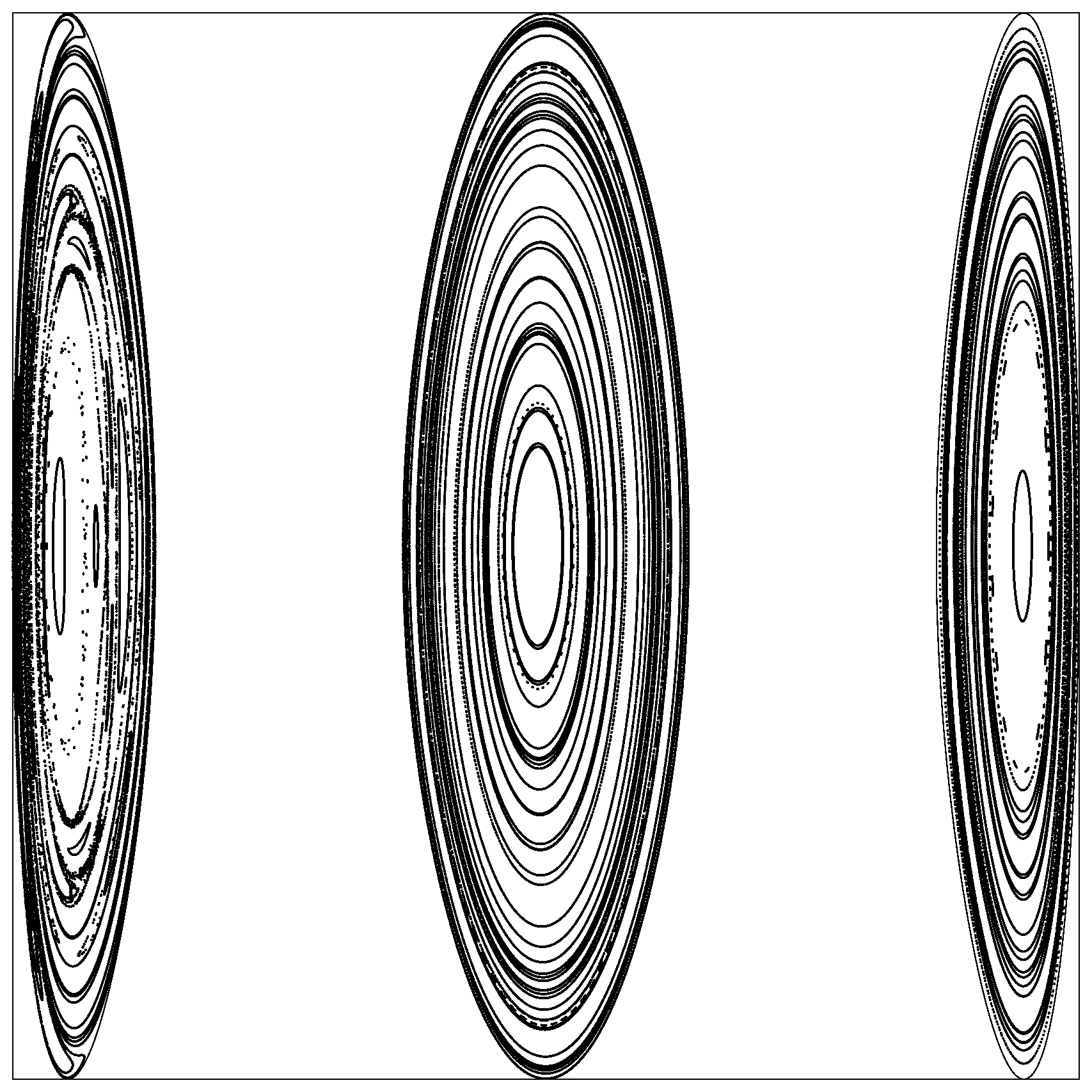
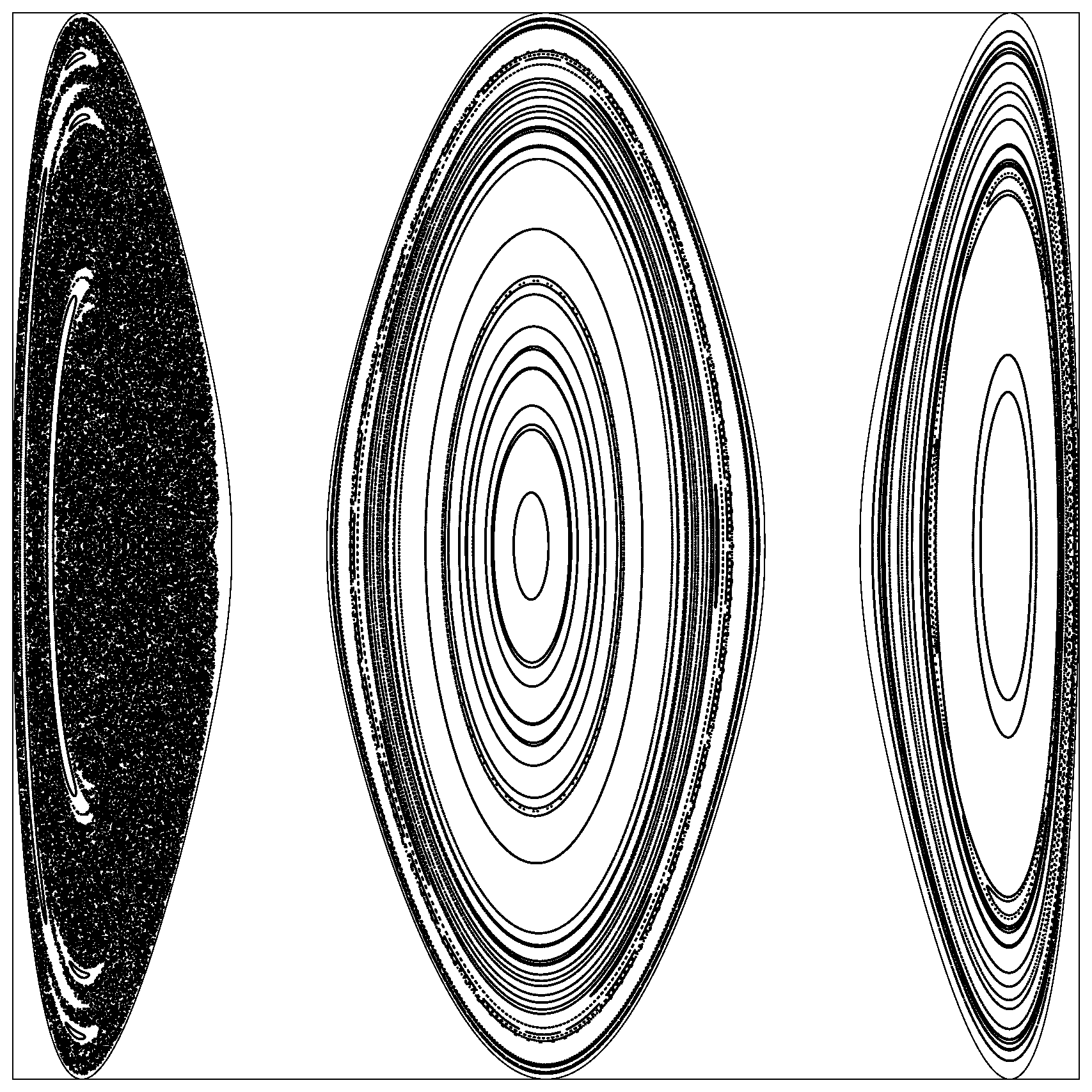
Figure 2.5: Level lines and Poincaré sections for $D_{5}$ and $D_{7}$ potentials .

The mixed state is observed for all considered potentials of umbilical catastrophes in the interval of energies $E_{cr}<E<E_{S}$ (here $E_{cr}$ is the critical energy of the transition to chaos in that local minimum, where chaos is observed at energies smaller than the saddle energy).

Chapter 3 Chaoticity Criteria for Multi-Well Potential

3.1 General formulation of the stochasticity criteria

As noted above, stochasticity is understood as a rise of statistical properties in a purely deterministic system due to local instability. According to this definition values of parameters of a dynamical system, under which local instability arises, are identified as regularity-chaos transition values. However, stochasticity criteria of such a type are not sufficient (their necessity poses a separate and complicated question), since loss of stability could lead to the transformation of one kind of regular motion to another. Despite this serious limitation, stochastic criteria in combination with numerical experiments facilitate an analysis of motion and essentially extend efficacy of numerical calculations.

3.2 Non-linear resonance overlap criterion

First among the widely used stochasticity criteria is the nonlinear resonances overlap criterion presented by Chirikov [15]. The essence of this criterion is easier to explain by the example of a one-dimensional Hamiltonian system, which is subjected to periodic perturbation

$$H=H_{0}(p,x)+Fx\cos\Omega t.$$

For the unperturbed system we can always introduce the action-angle variables $(I,\theta)$ in which

$$H=H_{0}(I)+\sum\limits_{k=-\infty}^{\infty}x_{k}(I)\cos(k\theta-\Omega t),$$ (3.1)

where

$$x_{k}(I)=\frac{1}{2\pi}\int\limits_{0}^{2\pi}d\theta e^{ik\theta}x(I,\theta).$$

In the new variables the scenario of stochasticity, on which resonances overlap criterion is based, is the following. An external periodic in time field induces a dense set of resonances in the phase space of a nonlinear conservative Hamiltonian system. The positions of these resonances $I_{k}$ are determined by the resonance condition between the eigenfrequency

$$\omega(I)=\frac{\partial H_{0}}{\partial I}$$

and the frequency of the external perturbation $\Omega$. For very weak the external fields the principle resonance zones remain isolated. As the amplitude $F$ of external field is raised, the widths $W_{k}$ of the resonance zones increase

$$W_{k}=\left.4\left(\frac{fx_{k}}{\omega^{\prime}(I)}\right)^{\frac{1}{2}}\right|_{I=I_{k}}$$

and at $F>F_{cr}$ resonances overlap. When this overlap occurs, i.e. under the condition

$$\frac{1}{2}(W_{k}+W_{k+1})=|I_{k}-I_{k+1}|,$$ (3.2)

it is said that there is transition to global stochastic behavior in the corresponding region of the phase space. The averaged motion of the system in the neighborhood of the nonlinear isolated resonance on the plane of the action-angle variables is similar to the particle behavior in the potential well. Isolated resonances correspond to isolated potential wells. The overlap of the resonances means, that the potential wells are close enough to make possible the random walk of a particle between these wells.

The outlined scenario can easily be ”corrected” for the description of the transition to chaos in the conservative system with several degrees of freedom. The condition of the resonance between the eigenfrequency and the frequency of the external field must be replaced by the condition of the resonance between the frequencies, which correspond to different degrees of freedom

$$\sum\limits_{i}m_{i}\frac{\partial H_{0}}{\partial I_{i}}=0.$$

The intensity of the interaction between different degrees of freedom, i.e. the measure of nonlinearity of the original Hamiltonian, acts as the amplitude of the external field in this case.

3.3 Stochastic layer destruction criterion

This method could be modified for systems with unique resonance [16]. In this case, the origin of the large-scale stochasticity is connected with the destruction of the stochastic layer near the separatrix of the isolated resonance. The main point of modification consists of the approximate reduction of the initial Hamiltonian in the neighborhood of the resonance to the Hamiltonian of the periodically perturbed nonlinear oscillator

$$H(\nu,x,\tau)=\frac{1}{2}\nu^{2}M\cos x-P\cos k(x-\tau).$$

The width of the resonance stochastic layer defined by [17]

$$W\sim\frac{\rho e^{-\frac{1}{\rho}}}{M\rho^{2k+1}}$$

where

$$\rho=\frac{2\sqrt{M}}{\pi k}.$$

If $P/M$ has an order $\rho^{s}$, then

$$W\sim\rho^{-\lambda}e^{-\frac{1}{\rho}}$$

where $\lambda=2k+1-s$. And when

$$\rho_{i}=\frac{1}{\lambda}\left(1-\frac{1}{\sqrt{1+\lambda}}\right)$$

function $W(\rho)$ has a bending flex point. Fast growth of $W$ allows us to define the threshold of the stochastic layer destruction as

$$\rho_{cr}=\frac{1}{\lambda^{2}}\left(\sqrt{1+\lambda}-1\right),$$

when the tangent line in point $\rho_{i}$ to the function $W(\rho)$ transects the $\rho$-axis.

Application of these criteria in the presence of strong nonlinearity (which is inevitable when considering multi-well potentials) encounters an obstacle: action-angle variables effectively work only in the neighborhood of the local minimum. Because of this, interest in methods based on direct estimation of trajectories divergence speed, arises. One of the criteria of such a type is so-called negative curvature criterion [18]. This criterion is based on the existence of the following scenario of the transition from regular to chaotic motion.

3.4 Negative curvature criterion

At low energies, the character of motion near the minimum of the potential energy, where the curvature is obviously positive, is periodic or quasiperiodic and is separated from the instability region by the zero curvature line. As the energy grows, the ”particle” will stay for some time in the negative curvature region of the PES where initially close trajectories exponentially diverge. After a long time these result in a motion which imitates a random one and is usually called stochastic. According to this stochastization scenario, the critical energy of the transition to chaos $E_{cr}$ coincides with the lowest energy on the zero curvature line

$$E_{cr}=U_{min}(K=0)$$

3.4.1 Results for one-well case

Now let s demonstrate the efficiency of negative curvature criterion on the example of one-parametric family of potentials

$$U(x,y;\mu)=\frac{1}{2}(x^{2}+y^{2})+xy^{2}+\mu x^{3}$$ (3.3)

With $\mu=-1$ potential (3.3) reduces to Hénon -Heiles potential and with $\mu=+1$ — to a separable one that is called anti- Hénon -Heiles potential. Interaction in any three-body system can be reduced to such a type of potential in the cubic approximation if its potential has the form [19]

$$U(x_{1},x_{2},x_{3})=U(x_{1}-x_{2})+U(x_{2}-x_{3})+U(x_{3}-x_{1}).$$

Gaussian curvature of the considered PES turns to zero at the points that satisfy the condition

$$-\frac{1}{\mu}y^{2}+(x-x_{0})^{2}=R_{0}^{2},$$

where

$$x_{0}=-\frac{1+\mu}{4\mu};\ R_{0}=\frac{1-\mu}{4\mu}.$$

When $\mu<0$, the zero-curvature line of (3.3) is an ellipse, which reduces to a circle for the Hénon -Heiles potential $(\mu=-1)$ (Fig.3.1)

$$x^{2}+y^{2}=\frac{1}{4}$$

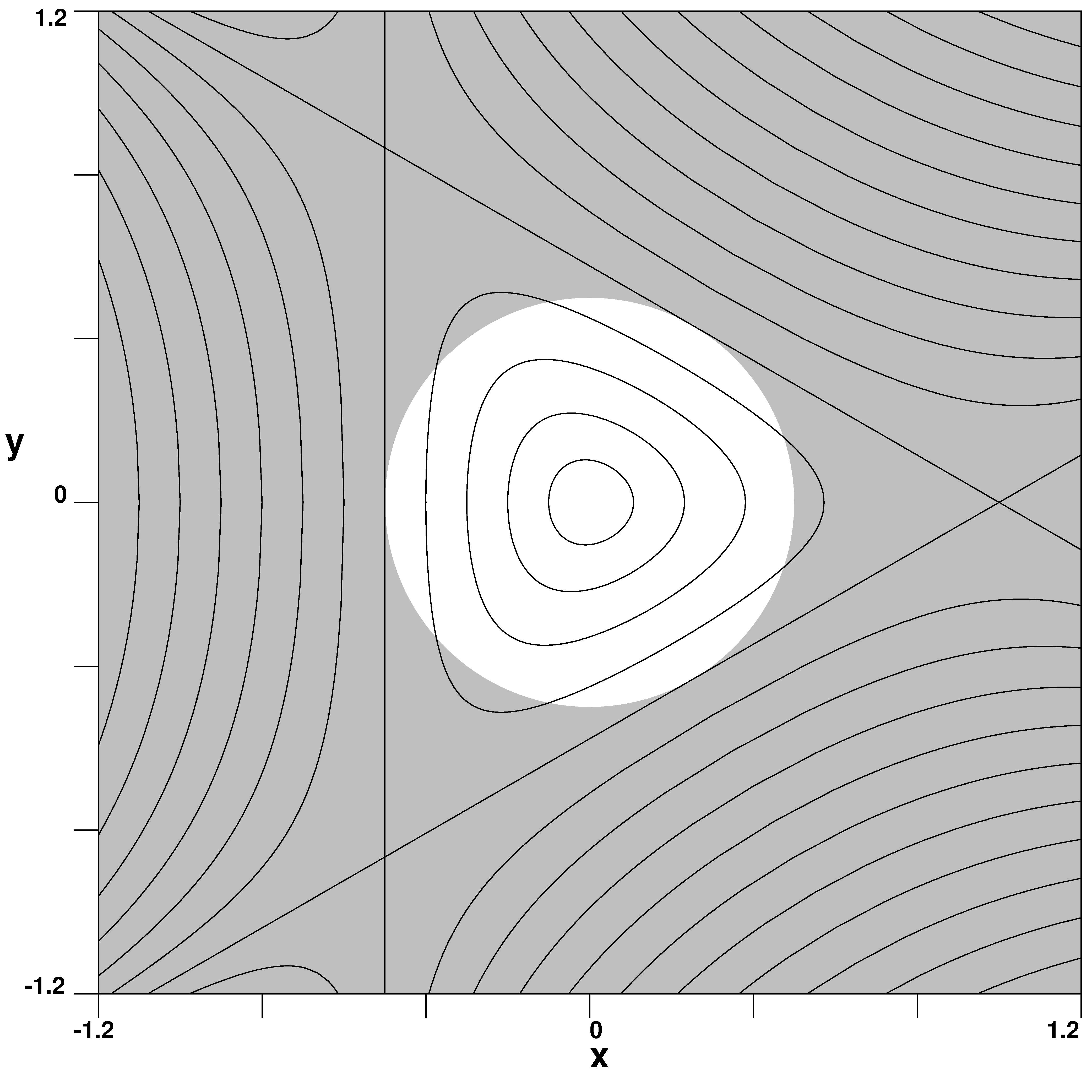
Figure 3.1: Level lines and negative curvature region (in grey) for Hénon- Heiles potential

On the zero-curvature line, energy is defined by the expression

$$U(K=0)=\frac{4}{3}\mu x^{3}+(1+\mu)x^{2}+\frac{1}{4}(2+\mu)x+\frac{1}{8},$$

and the minimal value of energy on the zero-curvature line is

$$U_{min}(K=0)=\frac{3-\mu}{48}.$$

According to the considered stochastization scenario, this value offers the critical energy when the transition from regular to chaotic motion occurs. For the Hénon -Heiles potential

$$U_{min}(K=0)=\frac{1}{12}.$$

This result is in good agreement with numerical integration of the equations of motion, which is presented on Fig.3.2 in the form of the Poincaré sections.

It is necessary to make one important remark. Analysis of numerical integration of the equations of motion (e.g. in the case of PSS) allows us to introduce the critical energy of the transition to chaos, determined as the energy such that part of phase space with chaotic motion exceeds a certain arbitrary chosen value. Similar uncertainty is connected with the absence of the sharp transition to chaos when energy increases. Therefore a certain caution is required for comparison of the ”approximate” critical energy obtained by numerical simulation, with the ”exact” value obtained with the help of analytical estimations, i.e. on the base of different criteria of stochasticity.

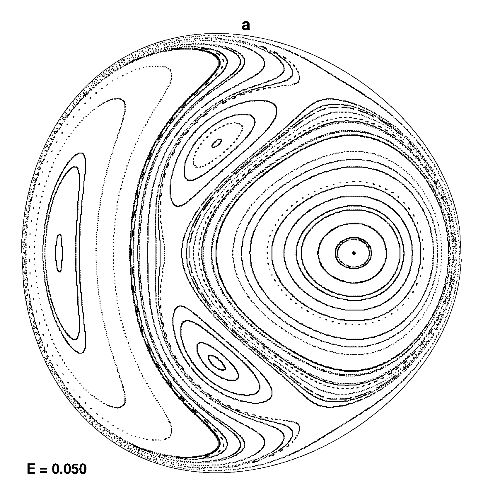
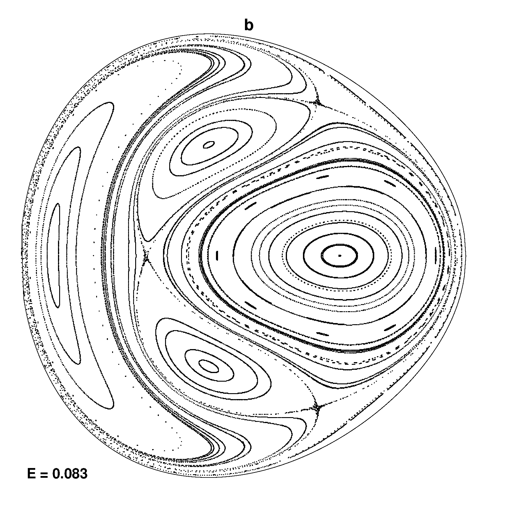
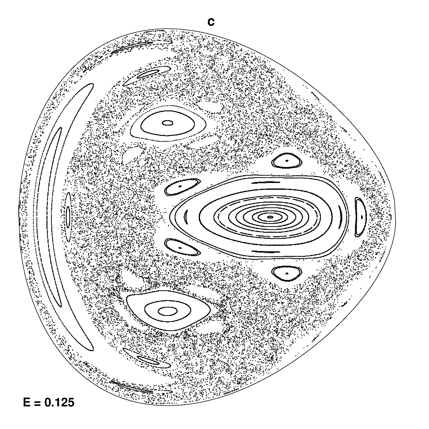
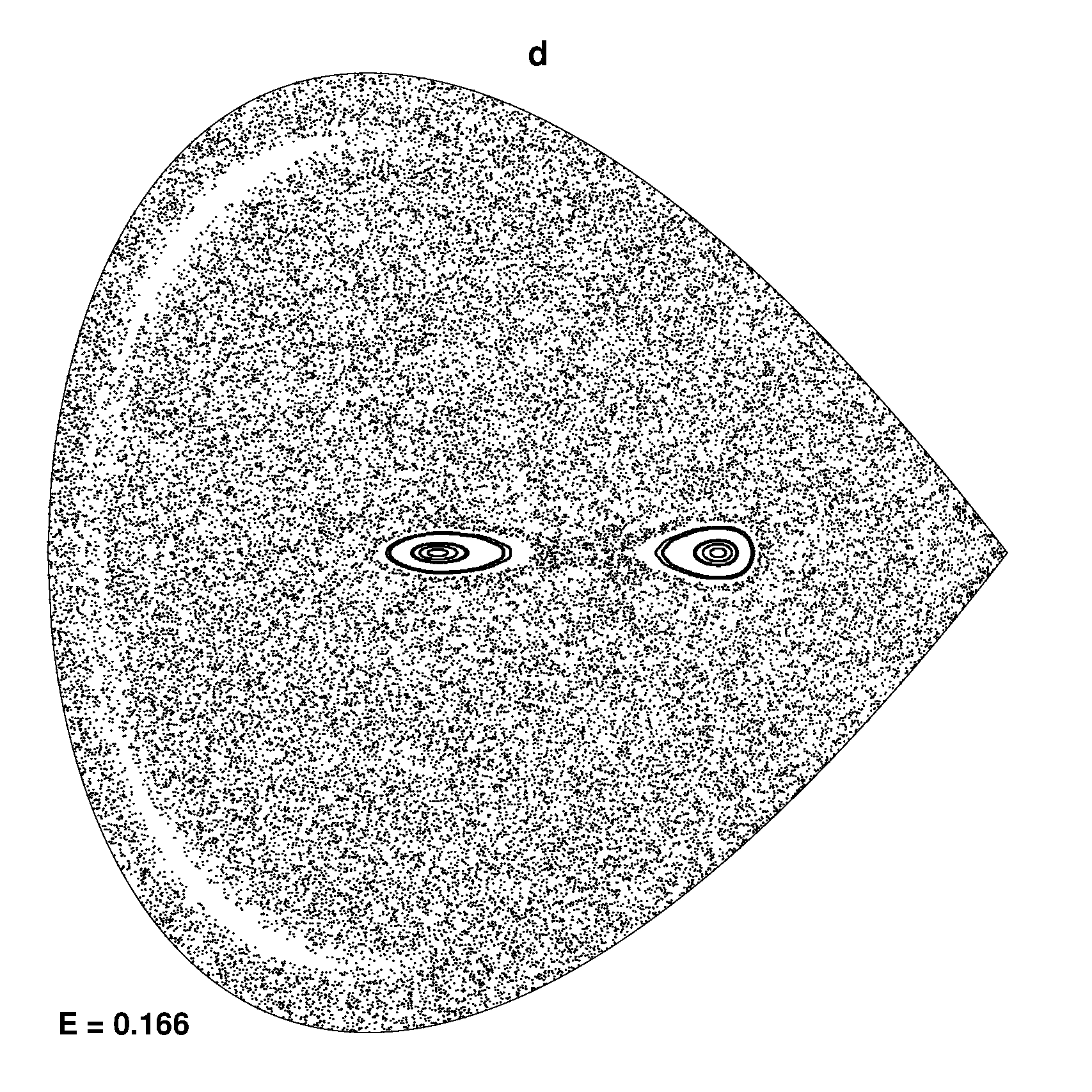
Figure 3.2: PSS for the Hénon -Heiles potential at $E<E_{S}/2$ (a), $E=E_{S}/2$ (b), $E_{S}/2<E<E_{S}$ (c), $E=E_{S}$ (d).

3.4.2 Failure for multi-well case

Negative curvature criterion allows us to obtain a number of interesting results in potentials with simple geometry (a single minimum) [20]. However, when passing to multi-well potentials, this criterion fails to work correctly. In particular, for the above mentioned potentials ($D_{5}$ and $D_{7}$), the structure of Gaussian curvature is similar in different wells. For example, for $D_{5}$ potential according to negative curvature criterion we get the same value of critical energy for both minima $E_{cr}\sim 5/9$, but chaotic motion is only observed in the left well (see Fig.2.5).

A natural question immediately arises: is it possible, using only geometrical properties of PES but not numerically solving equations of motion, to formulate an algorithm for finding the critical energy for single local minima in multi-well potential? We will try to answer this question below in the framework of the so-called geometrical approach [23, 21].

3.5 Geometrical approaches

The geometrical approach is based on application of differential geometry to study the chaotic dynamics of Hamiltonian systems. It turns out that as long as we consider the Hamiltonian of the form (2.2) we can restrict ourselves to the study of the configuration space without loosing information. Thus application of this method for the analysis of the features of Hamiltonian dynamics in multi-well potentials seems natural because the characteristic of the multi-well potential is formulated in terms of configurational space.

As is known, geodesics are among the main objects in Riemannian geometry. They are defined as the shortest curves that connect two points on a manifold. The manifold in its turn is defined by metrics. Having once fixed the metrics we thus define the distance on the manifold:

$$ds^{2}=g_{ik}dx^{i}dx^{k}.$$

We have the following condition for geodesics in this case:

$$\delta\int ds=0.$$ (3.4)

After variation we could obtain the differential equation for geodesics:

$$\frac{d^{2}q^{i}}{ds^{2}}+\Gamma^{i}_{\,jk}\frac{dq_{j}}{ds}\frac{dq_{k}}{ds}=0,$$ (3.5)

where $\Gamma^{i}_{\,jk}$ are Christoffel symbols.

Using variational principles it is possible to formulate Hamiltonian mechanics in a geometrical way. Let us consider this question more closely. A trajectory of dynamical system is defined according to Maupertuis [33] principle:

$$\delta\int\limits_{\gamma}2Tdt=0,$$ (3.6)

where $\gamma$ are all isoenergetic paths connecting end points, or according to Hamilton s principle:

$$\delta\int\limits_{t_{1}}^{t^{2}}Ldt=0.$$

To connect mechanics with Riemannian geometry we must choose the metrics that convert the expression under the integral into the length element. By such a procedure we will specify the manifold. Then trajectories will be geodesics on this manifold. We will call this CM – configurational manifold. This approach has an evident advantage: potential energy function includes all information about the system, so one needs to consider only configurational space but not phase space. Let s emphasize that Christoffel symbols in this approach act as counterparts of forces in ordinary mechanics and metrics — as a potential.

The simplest metric is the Jacobi metric. It has the form:

$$g_{ik}=2\left(E-V(q)\right)\delta_{ik}$$ (3.7)

By means of this metric Maupertuis principle (3.6) could be rewritten in the form equivalent to the condition for geodesics (3.4) so that trajectories are defined by equation (3.5). It could be shown that the geodesic equation (3.5) with Jacobi metric (3.7) leads to Newton s equations.

Having equations of motion we now could consider local instability in geometrical form. Let $\mathbf{q}$ and $\mathbf{q^{\prime}}$ be two nearby trajectories at $t=0$. Then let us define the deviation

$$J_{i}=q^{\prime}_{i}-q_{i}.$$

The dynamics of deviation are governed by the well known Jacobi-Levi-Civita (JLC) equation:

$$\frac{d^{2}J^{i}}{ds^{2}}+R^{i}_{\,jkl}\frac{dq^{j}}{ds}J^{k}\frac{dq^{l}}{ds}=0,$$ (3.8)

where $R^{i}_{\,jkl}$ is the curvature tensor. The two-dimensional case that we are interested in is very simple to consider because the only nonvanishing curvature tensor component is $R_{1212}$. To write JLC equation (3.8) explicitly we need to present local orthonormal basis. The simple choice is the following:

$$\mathbf{e}_{1}=\left(-\frac{dq^{2}}{ds},\frac{dq^{1}}{ds}\right),\ \mathbf{e}_{2}=\left(\frac{dq^{1}}{ds},\frac{dq^{2}}{ds}\right).$$

On this basis the deviation takes the form:

$$\mathbf{J}=\sum\limits_{i}\xi_{i}(s)\mathbf{e}_{i}(s)$$

It can be shown that in the two-dimensional case the JLC equation leads to two equations for deviation components on the chosen basis:

$$\begin{array}[]{c}\frac{d^{2}\xi_{1}}{ds^{2}}+\frac{1}{2}R\xi_{1}=0\\ \\ \frac{d^{2}\xi_{2}}{ds^{2}}=0\end{array}$$ (3.9)

where $R$ is scalar curvature. We can see that stability is determined by scalar curvature. For two-degrees-of-freedom systems Riemannian curvature has the form

$$R=\frac{(E-V)\Delta V+|\Delta V|^{2}}{2(E-V)^{2}}$$

where $\Delta V$ is positive for the considered potentials; thus Riemannian curvature is positive too. Due to this we cannot connect divergence of trajectories with negative Riemannian curvature.

Pettini et al. [21] point out that instability is caused by oscillations of positive curvature and has parametric nature. Calculations of deviation dynamics of regular and chaotic trajectories in Hénon -Heiles are presented in [23]. It is shown that, for regular trajectories, the normal component of deviation is bounded or grows linear in time, while for chaotic it grows exponentially. The initial conditions were chosen in specific areas in the Poincaré section. It is interesting to mention that initial conditions lying on the border of a regular island in section exhibit very slow exponential growth. This illustrates the so-called effect of sticky orbits.

Let us briefly discuss the behavior of deviation in equation (3.9 second order for $\xi_{1}$). In order to do that we need firstly to transform (3.9) to physical values, i.e. to time instead of interval [21]. This procedure leads to the following equation:

$$\frac{d^{2}\xi_{1}}{dt^{2}}-\frac{\dot{W}}{W}\frac{d\xi_{1}}{dt}+\left[\Delta V+\frac{(\nabla V)^{2}}{W}\right]\xi_{1}=0.$$ (3.10)

To simplify the equation and clarify its physical meaning, authors of paper [21] make the substitution:

$$\xi_{1}(t)=Y(t)\sqrt{W}$$ (3.11)

Obviously, $\xi_{1}(t)$ and $Y(t)$ have the same behavior in the meaning of stability hence $W(t)$ is bounded. Thus, using (3.11):

$$\frac{d^{2}Y}{dt^{2}}+\Omega(t)Y=0$$

with

$$\Omega(t)=\left[\Delta V+\frac{3(\nabla V)^{2}}{2W}\right]-\frac{3}{4W^{2}}\left[\dot{q}_{1}\frac{\partial V}{q_{1}}+\dot{q}_{2}\frac{\partial V}{q_{2}}\right]^{2}-\frac{1}{2W}\sum\limits_{i,k}\frac{\partial^{2}V}{\partial q_{1}\partial q_{2}}\dot{q}_{i}\dot{q}_{k}$$

Another geometrical approach, based on redefinition of covariant derivative was proposed by Kocharyan in [22]. In the two-dimensional case these two approaches lead to the same equations for deviation.

There are two possibilities for the solution to be unstable. The first case appears when $\Omega(t)$ is negative. The second possibility is parametric resonance. As was mentioned before, the second case is more actual since the Riemannian curvature is positive.

Fig.3.3 presents the distribution of $\langle\Omega(t)\rangle$ ($\langle\ldots\rangle$ means time averaged value) for an ensemble of $10^{4}$ trajectories in the chaotic well of potential $D_{5}$ with energy $E=E_{S}-0.1$.

Figure 3.3: The distribution of $\langle\Omega(t)\rangle$ for an ensemble of $10^{4}$ trajectories in the chaotic well of $D_{5}$ potential for $E=E_{S}-0.1$

As we can see, there is no trajectory with negative $\langle\Omega(t)\rangle$. Further, only $10\%$ of trajectories have somewhere $\Omega(t)<0$, but even for them $\langle\Omega(t)\rangle$ is positive. Although this is only a brief survey of the situation, we can expect that instability of the solution of (3.10) to have parametric nature.

As was mentioned earlier, stochasticity criterion must derive critical energy. However it was pointed out by Pettini et al. that we must know all information about curvature oscillations to consider parametric instability. So, dynamical calculations are unavoidable in this investigation. Nevertheless, we could derive purely geometrical criterion by introduction of additional coordinates. Let us rewrite the JLC equation in the form which does not depend on dimensionality of the manifold:

$$\frac{1}{2}\frac{d^{2}\left\|\mathbf{J}\right\|^{2}}{ds^{2}}+K^{(2)}(\mathbf{J},\mathbf{v})\left\|\mathbf{J}\right\|^{2}-\left\|\frac{d}{ds}\mathbf{J}\right\|^{2}=0$$

where $K^{(2)}(\mathbf{J},\mathbf{v})$ is the so-called sectional curvature:

$$K^{(2)}(\mathbf{J},\mathbf{v})=R_{iklm}\frac{J^{i}}{\left\|\mathbf{J}\right\|}\frac{dq^{k}}{ds}\frac{J^{l}}{\left\|\mathbf{J}\right\|}\frac{dq^{m}}{ds}$$

and $\langle\mathbf{J},\mathbf{v}\rangle=0$. Note that the point where $K^{(2)}(\mathbf{J},\mathbf{v})<0$ is unstable. Since there are more than one sectional curvatures for the case $N>2$, we could connect instability with the negative sign of some of them. It is assumed that negativity of some of the sectional curvatures is sufficient condition for the rise of instability. One of the enlarged metrics is the Eisenhart metric:

$$ds^{2}_{E}=(g_{E})_{\mu\nu}dq^{\mu}dq^{\nu}=a_{ij}dq^{i}dq^{j}-2V(\mathbf{q})(dq^{0})^{2}+2dq^{0}dq^{N+1}$$

where $a_{ij}$ is the kinetic energy matrix. The additional coordinates are $q^{0}=t$ and $q^{N+1}$ (the latter is connected with action). The nonvanishing components of curvature tensor are

$$R_{0i0j}=\frac{\partial^{2}V}{dq^{i}dq^{j}}.$$

Pettini et al. [23] considered $K^{(2)}(\mathbf{J},\mathbf{v})$ on the constant energy surface for vectors

$$\mathbf{J}=(0,\dot{q}_{2},-\dot{q}_{1},0),\ \mathbf{v}=(1,\dot{q}_{1},\dot{q}_{2},\dot{q}_{3}).$$

Thus $K^{(2)}(\mathbf{J},\mathbf{v})$ takes on the form:

$$K^{(2)}(\mathbf{q},\mathbf{\dot{q}})=\frac{1}{2(E-V(\mathbf{q}))}\left(\frac{\partial^{2}V}{\partial q_{1}^{2}}\dot{q}_{2}^{2}+\frac{\partial^{2}V}{\partial q_{2}^{2}}\dot{q}_{1}^{2}-\frac{\partial^{2}V}{\partial q_{1}\partial q_{2}}\dot{q}_{1}\dot{q}_{2}\right)$$

This value is easy to calculate at any point of phase space. In [23] the averaged value of $K^{(2)}(\mathbf{J},\mathbf{v})$ is introduced. It is shown that for Hénon -Heiles potential there exists a correlation between chaotic trajectories relative measure and averaged value of sectional curvature. This approach correctly predicts the value of critical energy.

The case of multi-well potential is more complex. It is necessary to clarify whether this condition is sufficient for the development of chaoticity or not; clearly speaking we needs to answer the question, does the presence of negative curvature parts on CM always lead to chaos? Potentials with mixed state are a very convenient model for investigation of this question, since there exist both regimes of motion. So, we need to study, how the structure of $K^{(2)}(\mathbf{J},\mathbf{v})$ differs in different wells. For that we calculate in [24] a part of phase space with negative curvature as a function of energy, i.e. a volume of phase space where $K^{(2)}(\mathbf{J},\mathbf{v})<0$ referred to the total volume:

$$\mu(E)=\frac{\int d\mathbf{q}d\mathbf{p}\Theta(-K^{(2)})\delta(H(\mathbf{q},\mathbf{p})-E)}{\int d\mathbf{q}d\mathbf{p}\delta(H(\mathbf{q},\mathbf{p})-E)}.$$

We carried out calculations for two potentials: $D_{5}$ and $D_{7}$. Calculations of $\mu(E)$ (Fig.3.4) show that there are parts, where $K^{(2)}(\mathbf{J},\mathbf{v})<0$ in all wells, but nevertheless chaos exists only in one well. Moreover, for the well with chaotic motion, function $\mu(E)$ gives the correct value of critical energy — at this energy $\mu(E)$ becomes positive.

Figure 3.4: Function $\mu(E)$ for $D_{5}$ (a) and $D_{7}$ (b) potentials. $\mu(E)$ for chaotic wells are represented by dotted lines, for regular — by triangles.

The situation with regular wells is more complicated. Although part of phase space, where $K^{(2)}(\mathbf{J},\mathbf{v})<0$, is nonzero, chaos in the well does not exist. This can be viewed on the Poincaré sections. For comparison in Fig.3.5 part of CS with negative Gaussian curvature ($\mu_{G}$) is shown. We can see that structure of negative Gaussian curvature is similar to the $K^{(2)}(\mathbf{J},\mathbf{v})$-structure.

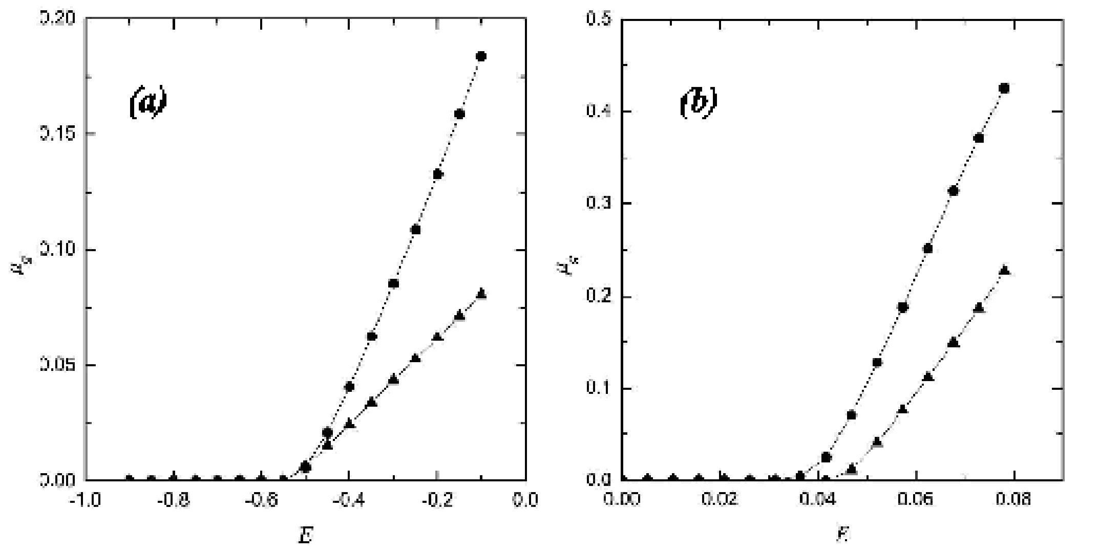
Figure 3.5: Function $\mu_{G}(E)$ for $D_{5}$ (a) and $D_{7}$ (b) potentials.

Investigation of the curvature of the manifold, as we can see from the above cited data, does not give a plain method for identification of chaos in any minimum, especially if there exist both regular and chaotic regimes of motion. It is impossible to determine a priori whether chaos existed in the system without using dynamical description (in our case which are Poincaré sections). Nevertheless, we can efficiently use geometrical methods for investigation of chaos in multi-well potentials. In thee potentials considered above chaos exists only in wells, which have two details: a non-zero part of negative curvature on the manifold and at least one hyperbolic point in the Poincaré section. According to this, we can use the following method for identification of chaos and calculation of critical energy. At the first step the Poincaré section at low energy is drawn for the well and the presence of the hyperbolic point is detected. The quantity $\mu(E)$ must then be calculated (or the part of CS with negative Gaussian curvature). The value of energy at which $\mu(E)$ becomes positive could be associated with critical energy. If there are no hyperbolic points in the section than chaos does not exist in the well. Consequently, geometrical methods could be efficiently used for determination of critical energy in complex potentials and identification of chaos in general. However, we must carefully use these methods and combine them with qualitative methods, such as Poincaré sectioning method.

3.6 Normal forms

The structure of the Poincaré surfaces of section can be reproduced without resorting to the numerical solution of the equations of motion. For this, let us use the method of treating non separable classical systems that was originally developed by Birkhoff [25] and later was extended by Gustavson [26].

Every two-dimensional Hamiltonian near equilibrium point can be represented in polynomial form as follows

$$\begin{array}[]{c}H(\mathbf{p},\mathbf{q})=H^{(2)}(\mathbf{p},\mathbf{q})+V(\mathbf{q}),\\ H^{(2)}(\mathbf{p},\mathbf{q})=\sum\limits_{\nu=1}^{2}\frac{1}{2}\omega_{\nu}^{2}(p_{\nu}^{2}+q_{\nu}^{2}),\\ V(\mathbf{q})=\sum\limits_{j\leq 3}V_{j_{1}j_{2}}q_{1}^{j_{1}}q_{2}^{j_{2}},\\ \mathbf{q}=(q_{1},q_{2}),\ \mathbf{p}=(p_{1},p_{2}).\end{array}$$

The procedure of reducing to normal form depends on whether the frequencies $\omega_{\nu}$ are commensurable or not. If they are incommensurable then there exists a canonical transformation $(\mathbf{q},\mathbf{p})\rightarrow(\mathbf{\xi},\mathbf{\eta})$ such that in variables $(\mathbf{\xi},\mathbf{\eta})$ Hamiltonian $\Gamma(\mathbf{\xi},\mathbf{\eta})$ will be a function of only two combinations

$$I_{\nu}=\frac{1}{2}\left(\xi_{\nu}^{2}+\eta_{\nu}^{2}\right),\ \nu=1,2.$$

In other words, the Birkhoff normal form is an expansion of the original Hamiltonian over two one-dimensional harmonic oscillators

$$H(\mathbf{p},\mathbf{q})\rightarrow\Gamma(\mathbf{\xi},\mathbf{\eta})=\omega_{1}I_{1}+\omega_{2}I_{2}+\sum\limits_{\mu,\nu}a_{\mu\nu}I_{\mu}I_{\nu}+\ldots$$

If the frequencies $\omega_{\nu}$ are commensurable, i.e. if there exist resonance relations of the type $m\omega_{1}+n\omega_{2}$, the normal form becomes more complicated and will contain apart from $I_{\nu}$ other combinations of variables $\xi_{\nu}$ and $\eta_{\nu}$ as well. Such extended normal forms are called the Birkhoff-Gustavson normal forms.

We cite as an example the Birkhoff normal form (up to the terms of the sixth degree with respect to $(\mathbf{\xi},\mathbf{\eta})$) for the umbilical catastrophe $D_{5}$ in the neighborhood of right minimum:

$$\begin{array}[]{c}H(I_{1},I_{2})=2.613I_{1}+2I_{2}-0.219I_{1}I_{2}-0.017I_{1}^{2}-0.375I_{2}^{2}-\\ -0.005I_{1}^{3}-0.028I_{1}^{2}I_{2}-0.122I_{1}I_{2}^{2}-0.133I_{2}^{3}\end{array}$$

The reduction of the Hamiltonian to the normal form solves the problem of the construction of a full set of approximate integrals of motion. The solution of the equations

$$\begin{array}[]{c}H(p_{x},p_{y},x,y)=E\\ H(p_{x},p_{y},x,y)=I_{0}\\ x=const\end{array}$$

allows us to find the set of intersections of the phase trajectory with the selected plane ($x=const$) and to reconstruct the structure of PSS.

The PSS for the quadrupole oscillations of nuclei ${}^{74}Kr$, which are constructed in such a way, are shown in Fig.3.6. The qualitative coincidence of topology of PSS calculated with the help of normal forms and the numerical integration of the equation of motion is noteworthy.

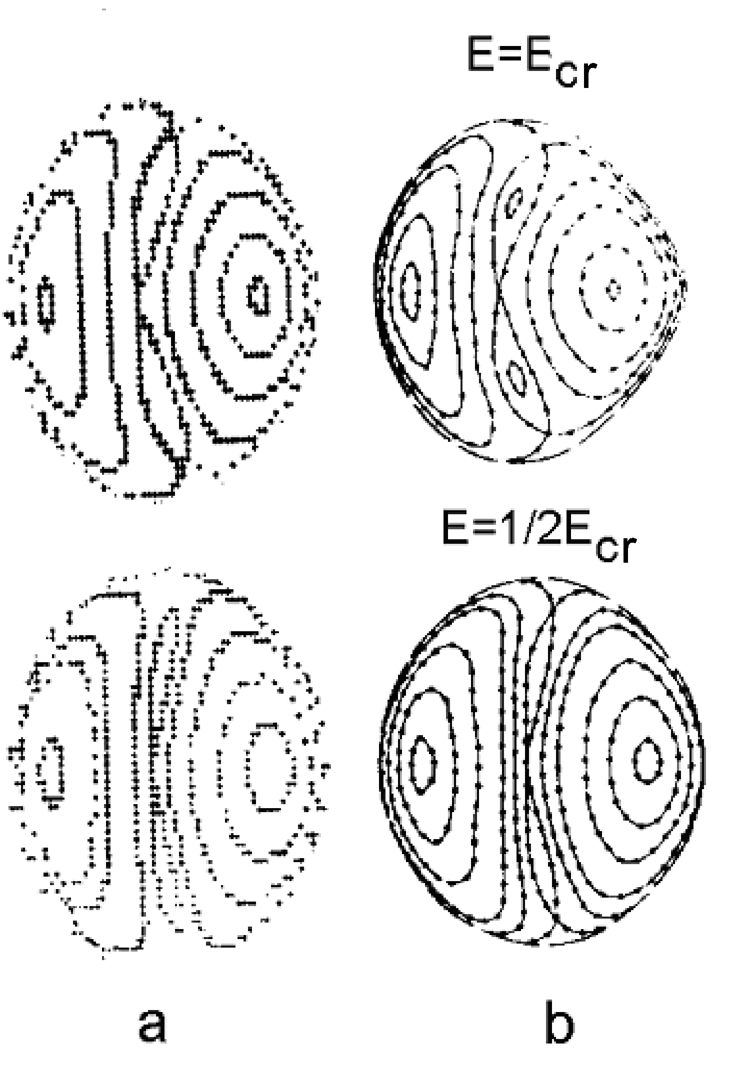
Figure 3.6: The PSS for different values of energy for central minimum of ${}^{74}Kr$ obtained a) by numerical integration of equation of motion, b) by normal forms.

Having failed in an attempt to formulate adequate criterion of stochasticity that is based on the estimation of the rate of divergence of the two initially close trajectories (nevertheless, we do not doubt the existence of such criterion), let us now return to the resonance overlap criterion. By means of it we will try to understand the differences in the phase space structure of the different local minima that realize different dynamical regimes.

As an example let us consider the application of this criterion to the dynamics that are generated by the potential of umbilical catastrophe $D_{5}$. Accordingly the Hamiltonian in the reference frame connected with left (upper sign) and right (lower sign) well has the form

$$H=\frac{1}{2}(\dot{x}^{2}+\omega_{1}^{2}x^{2})+\frac{1}{2}(\dot{y}^{2}+\omega_{2}^{2}y^{2})+xy^{2}\mp\sqrt{2}x^{3}+\frac{1}{4}y^{4}$$ (3.12)

where

$$\omega_{1}=\sqrt{2(2\mp\sqrt{2})};\ \omega_{2}=2.$$

Now we make a canonical transform to the action-angle variables

$$\begin{array}[]{cc}x=\sqrt{\frac{2I_{1}}{\omega_{1}}}\cos\varphi_{1};&y=\sqrt{\frac{2I_{2}}{\omega_{2}}}\cos\varphi_{2};\\ \dot{x}=\sqrt{2I_{1}\omega_{1}}\sin\varphi_{1};&\dot{x}=\sqrt{2I_{2}\omega_{2}}\sin\varphi_{2}.\end{array}$$ (3.13)

Thus Hamiltonian (3.12) takes the form

$$\begin{array}[]{c}H(I_{1},I_{2},\varphi_{1},\varphi_{2})=H_{0}(I_{1},I_{2})+\sum\limits_{n_{1},m_{2}\in\Lambda}f_{m_{1}m_{2}}\cos(m_{1}\varphi_{1}+m_{2}\varphi_{2})\\ \Lambda:[0,1],[0,2],[0,3],[0,4],[2,1],[2,-1]\end{array}$$ (3.14)

where

$$\begin{array}[]{c}H_{0}(I_{1},I_{2})=I_{1}\omega_{1}+I_{2}\omega_{2}+\frac{3}{8}\frac{I_{2}^{2}}{\omega_{2}^{2}}-1\\ f_{01}=\frac{I_{1}}{\omega_{1}}\left(\frac{2I_{2}}{\omega_{2}}\right)^{1/2}\pm 3\left(\frac{I_{2}}{\omega_{2}}\right)^{3/2}\\ \begin{array}[]{cc}f_{02}=\frac{1}{2}\frac{I_{2}^{2}}{\omega_{2}^{2}};&f_{03}=\pm\left(\frac{I_{2}}{\omega_{2}}\right)^{3/2}\\ f_{04}=\frac{1}{8}\frac{I_{2}^{2}}{\omega_{2}^{2}};&f_{21}=f_{2,-1}=\frac{1}{2}\frac{I_{1}}{\omega_{1}}\left(\frac{2I_{2}}{\omega_{2}}\right)^{1/2}\end{array}\end{array}$$

An item with indexes $r=(r_{1},r_{2})$ is called the resonance for a given value of energy $E$ if there exist action variables $(I_{1}^{r},I_{2}^{r})$ such, that $E=H_{0}(I_{1}^{r},I_{2}^{r})$ and

$$r_{1}\bar{\omega}_{1}(I_{1}^{r},I_{2}^{r})+r_{2}\bar{\omega}_{2}(I_{1}^{r},I_{2}^{r})=0$$

where

$$\bar{\omega}_{i}=\frac{\partial H_{0}}{\partial I_{i}},\ i=1,2.$$

If the system is far enough from resonance, i.e. for all $(m_{1},m_{2})$

$$|m_{1}\bar{\omega}_{1}+m_{1}\bar{\omega}_{1}|\gg f_{m_{1}m_{2}},$$

then avoiding the small denominator problem we could make a canonical transform to new action-angle variables thus eliminating angle dependence in lower orders under some small parameter. This procedure results in the redefinition of the integrable part $H_{0}$ of the initial Hamiltonian and enlargement of the set $\Lambda$ of angle-dependent terms. After that we could encounter one of following three possibilities:

1. resonance terms are still absent in the considered region;

2. the single resonance term arises;

3. multiple resonances arise.

In the first case we should execute a new canonical transformation and keep carrying out the procedure until case 2 or 3 appears. In the second case critical energy of the transition to large-scale stochasticity could be defined with stochastic layer destruction criterion [16]. And finally in the third case we could use the Chirikov’s resonance overlap criterion [15] to determine the critical energy.

Small unbalancing near resonance

$$|m_{1}\bar{\omega}_{1}+m_{1}\bar{\omega}_{1}|\leq f_{m_{1}m_{2}}$$

could be compensated by higher order terms that have arisen from the repeated canonical transformation of the non-resonance terms. In the Hamiltonian (3.14) the term $[2,-1]$ is subjected to condition (3.13), and the considered procedure leads to

$$\begin{array}[]{c}H_{0}(I_{1},I_{2})=I_{1}\omega_{1}-1+\frac{3}{8}\frac{I_{2}^{2}}{\omega_{2}^{2}}-\frac{4\omega_{1}+5}{32\omega_{1}^{2}(\omega_{1}+1)}I_{1}^{2}+\\ +\left[\pm\frac{3\sqrt{2}}{2}-\frac{1}{\omega_{1}(\omega_{1}+1)}\right]\frac{I_{1}I_{2}}{8\omega_{1}}.\end{array}$$

In the left well let us take into account only two terms: resonance

$$\frac{1}{2}\frac{I_{1}}{\omega_{1}}\left(\frac{2I_{2}}{\omega_{2}}\right)^{1/2}\cos(2\varphi_{1}-\varphi_{2})$$

and ”shaking” ones [16]:

$$\frac{\sqrt{2}}{64\omega_{1}}\left[\frac{3}{\omega_{1}+1}+\frac{1}{\omega_{1}}\right]I_{1}I_{2}\cos(2\varphi_{1}-2\varphi_{2}).$$

After this direct application of the stochastic layer destruction criterion leads to the value of the critical energy in the left well

$$E_{cr}\simeq-0.51$$

This value is in a good agreement with numerical integration results and in qualitative agreement with the estimation obtained by negative curvature criterion $E_{cr}=-5/9$. Straightforward analysis of the integrable part of the Hamiltonian (3.14) shows that there are no resonance terms in the right well. Thus transition to large-scale stochasticity in the right well could be attained only when passing the saddle energy. This fact is in full agreement with numerical results.

Resonance overlap criterion allows better understanding of the mechanism of the above mentioned regularity-chaos-regularity transition that exists in any (multi- or single-well) potential with a localized region of instability. Let us use similarity in structure of phase space of the considered two-dimensional autonomous Hamiltonian system with the compact region of negative Gaussian curvature and one-dimensional system with periodic perturbation (3.1) [27].

The behavior of the widths of the resonances

$$W_{k}\equiv\frac{1}{2}(W_{k+1}+W_{k}),$$

and the distances between them

$$\Delta I_{k}\equiv|I_{k+1}-I_{k}|$$

as a function of the resonance number is simplest when the satisfaction of resonance overlap condition (3.2) for number $k_{1}$ (at a fixed level of the external perturbation) guarantees that this condition holds for arbitrary $k>k_{1}$. This is precisely the situation, that prevails in the extensively studied systems of a Coulomb potential [30] and a square well [31] subjected in each case to a monochromatic perturbation. In the former case we have $\bar{W}_{k}\approx k^{1/6}$ and $\Delta I_{k}\approx k^{-2/3}$, while in the latter we have $\bar{W}_{k}\approx k^{-1}$ and $\Delta I_{k}\approx[k(k+1)]^{-1}$. As can be seen from Fig.3.7 there is R-C transition (we will call this transition a ”normal” transition) for both the Coulomb problem and a square well, since there exists a unique point $k_{1}$ such that at $k>k_{1}$ the condition $\bar{W}_{k}>\Delta I_{k}$ always holds. The motion is therefore chaotic. However, as the behavior of the widths of the resonances and of the distances between them as a function of the resonance number becomes more complicated, we can allow the appearance of an additional intersection point and thus a new transition: C-R transition, which we will call ”anomalous”. There is also the exotic possibility of the intermitting occurrence of the regular and chaotic regions in the phase space.

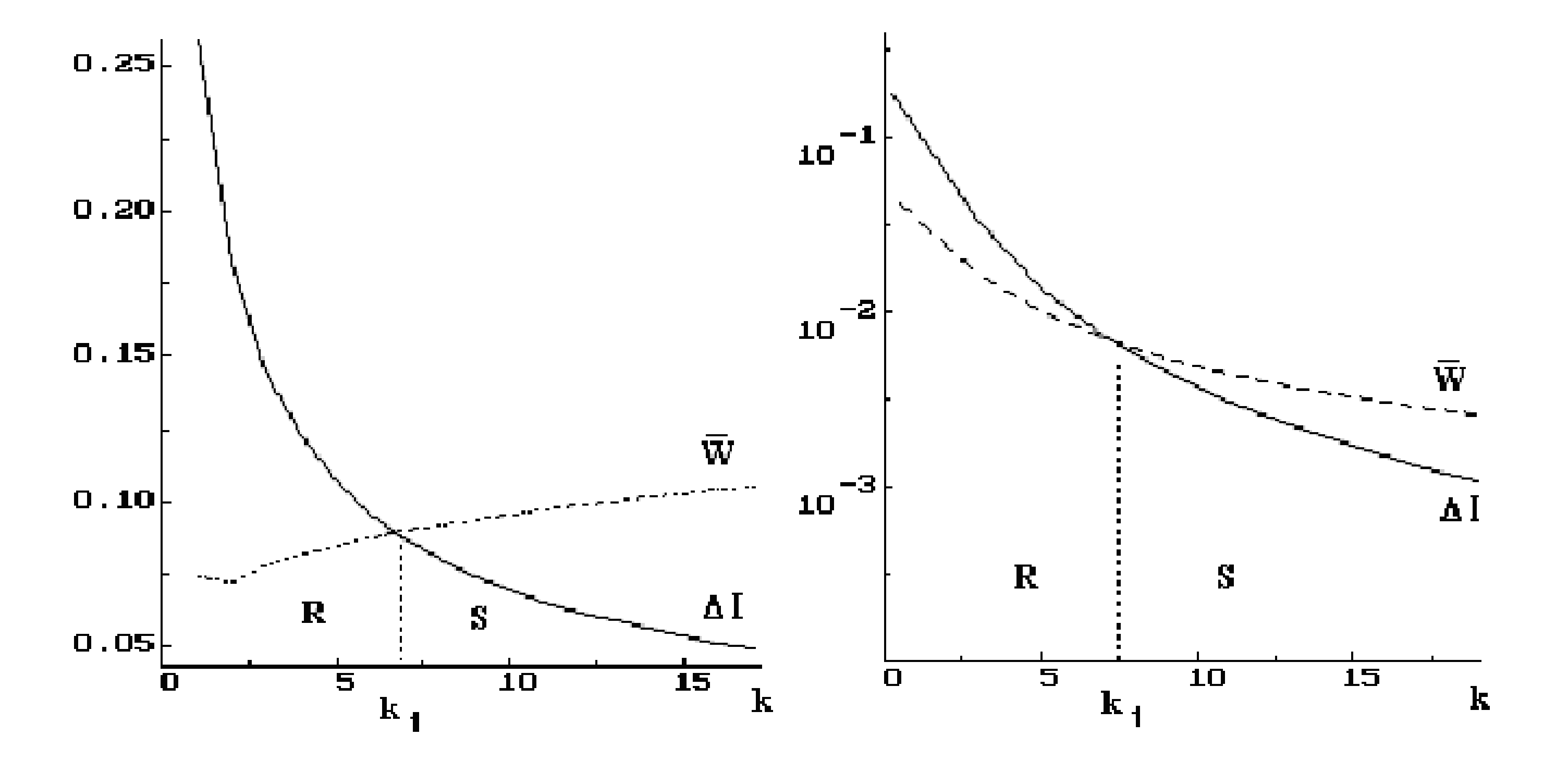
Figure 3.7: The resonant spacing $\Delta I_{k}$ (solid lines) and the mean widths $\bar{W}_{k}$ (dashed lines) as functions of the resonance numbers $k$. On the left: for one-dimensional Coulomb, on the right: for square-well potential. The critical point $k_{1}$ separates the regular range ($R$) from the chaotic one ($S$).

We demonstrate that an anomalous C-R transition occurs in a simple Hamiltonian system: an anharmonic oscillator, subjected to a monochromatic perturbation [32, 27]. The dynamics of such a system is generated by the Hamiltonian

$$H(p,x,t)=H_{0}(p,x)+Fx\cos\Omega t$$ (3.15)

where the unperturbed Hamiltonian is

$$H_{0}(p,x)=\frac{p^{2}}{2m}+Ax^{n}=E,\ (n=2l,\ l>1)$$ (3.16)

The considered system fills a gap between two extremely important physical models: the harmonic oscillator ($n=2$) and the square well ($n=\infty$).

In terms of action-angle variables $(I,q)$, the Hamiltonian $H_{0}(p,x)$ (3.16) becomes [27]

$$H_{0}(I)=\left(\frac{2\pi}{\alpha G(n)}I\right)^{\alpha},\ G(n)=\frac{2\sqrt{2\pi m}\Gamma\left(1+\frac{1}{n}\right)}{A^{\frac{1}{n}}\Gamma\left(\frac{1}{2}+\frac{1}{n}\right)},\ \alpha=\frac{2n}{n+2}$$

The resonant values of the action $I_{k}$ that can be found from the conditions

$$k\omega(I_{k})=\Omega,\ \omega(I)=\frac{dH_{0}}{dI}$$

are

$$I_{k}=\alpha\left(\frac{G(n)}{2\pi}\right)^{2n\beta}\left(\frac{\Omega}{k}\right)^{\frac{2n\alpha}{\beta}},\ \beta=\frac{1}{n-2}.$$

A classical analysis, based on the resonance overlap condition, leads to the following expression for the critical amplitude of the external perturbation

$$F_{k}^{cr}=2^{(2-3n)\beta}\frac{1}{4n}\frac{\alpha^{2}}{\beta}\frac{1}{x_{k}}\left(\frac{G(n)}{2\pi}\right)^{2n\beta}\Omega^{2n\beta}k^{4\beta}\left[k^{(n+2)\beta}-(k+1)^{(n+2)\beta}\right],$$ (3.17)

where $x_{k}$ is the Fourier component of the coordinate $x(I,\theta)$. Expression (3.17) solves the problem of reconstructing the structure of the phase space for arbitrary values of the parameters.

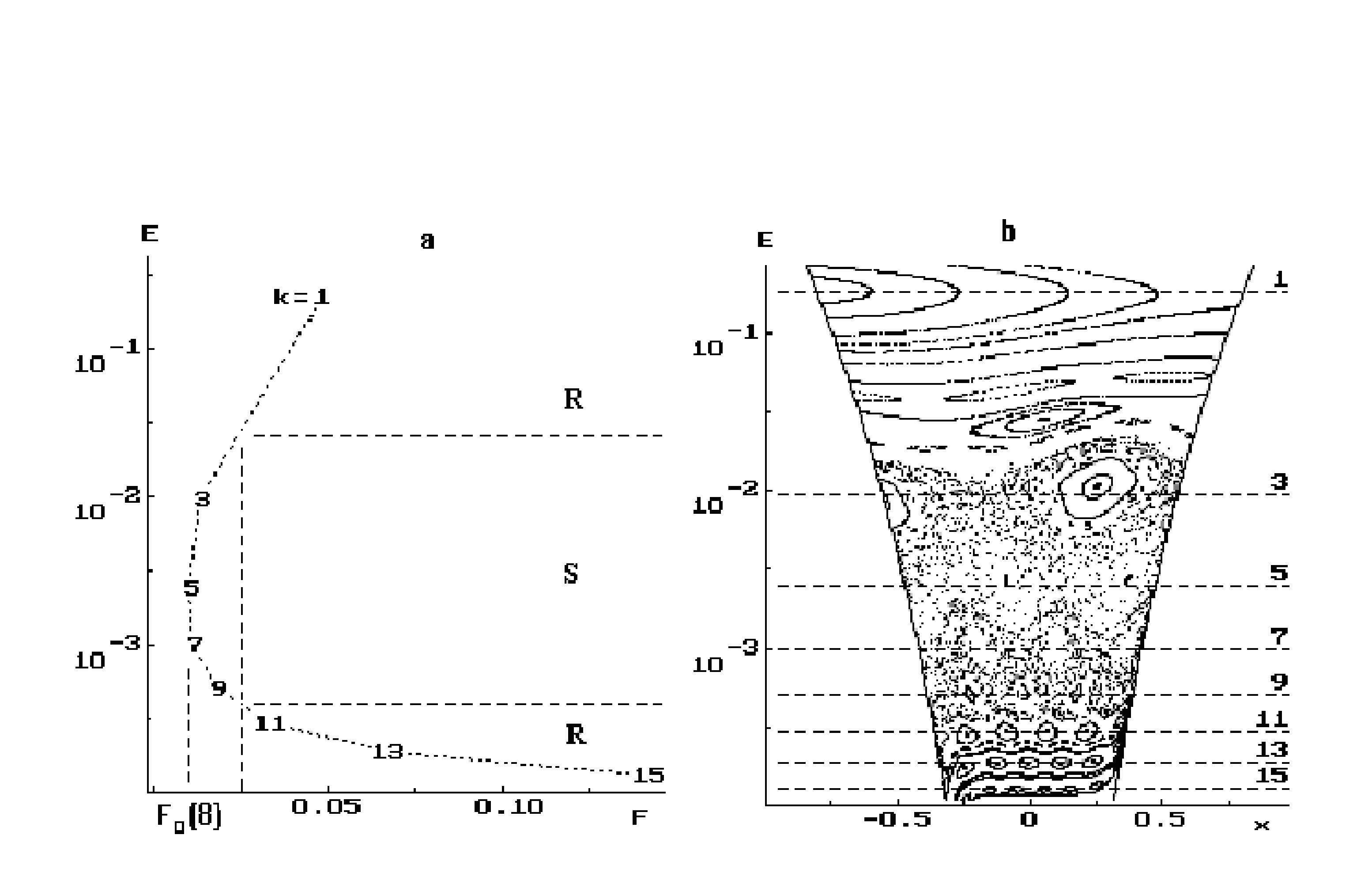
Figure 3.8: a) The phase diagram of the R-C-R transition for Hamiltonian (3.15): resonance energy $E_{k}$ versus the critical values of the external perturbation $F(n=8)$. b) The snap-shot $E(x)$ confirms that the anomalous C-R transition occurs.

The phase diagram in Fig.3.8a can be used to determine, at the fixed level of the external perturbation, the energy intervals of regular and chaotic motion. The snap-shot of $E(x)$ at the right in Fig.3.8b confirms that an anomalous C-R transition occurs. We can clearly see isolated nonlinear resonances which persist at large values of $k$, and near which the motion remains regular. The reason for this anomaly is explained by Fig.3.8. The plots of the resonance widths and the distances between resonances in this figure demonstrate that there are two rather than one intersection points: $k=k_{1}$ and $k=k_{2}$. Consequently, there is an anomalous C-R transition.

Thus, for $1D$ system with periodic perturbation R-C-R transition can be observed just as in the case of a $2D$ autonomous Hamiltonian system. The reason for the additional transition in both cases is common: the localized region of instability. In the first case this reason is the localized domain of overlap resonances, while in the second one this reason is the localized domain of negative Gaussian curvature.

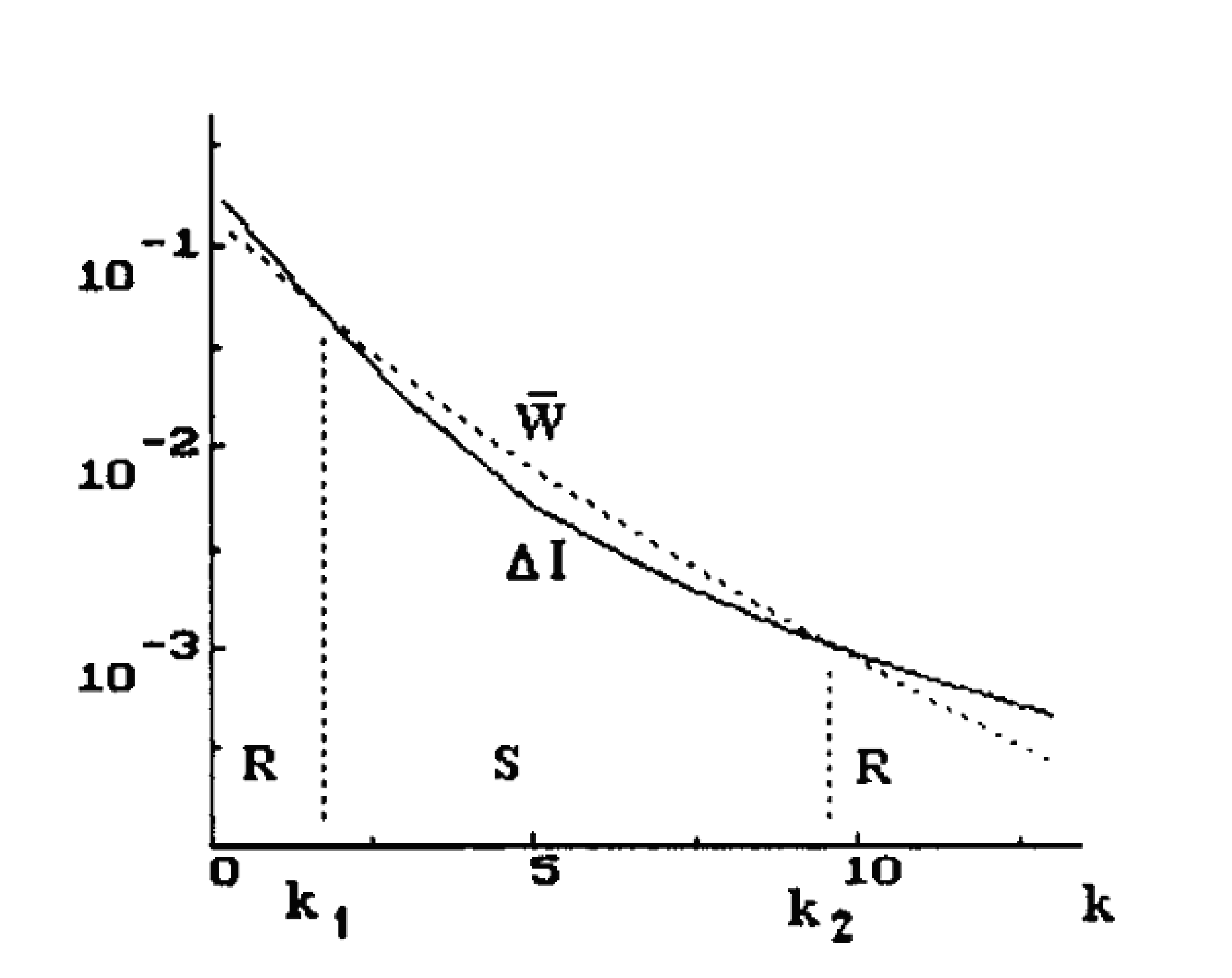
Figure 3.9: The resonant spacings $\Delta I_{k}$ (solid line) and mean widths $\bar{W}_{k}$ (dashed line) as functions of the resonance numbers $k(n=8)$. There are two critical points $k_{1},k_{2}$ . The second critical point corresponds to the anomalous C-R transition.

Chapter 4 Quantum Manifestations of Classical Stochasticity — Formulation of the Problem

After almost a hundred years of development, quantum mechanics became a universal picture of the world. On any observable scales of energy we could not find any violations of quantum mechanics. But this does not mean that from time to time quantum mechanics does not confront another challenge. The problem that arose at the face of quantum mechanics in the second part of the last century is called quantum chaos. The essence of the problem is the fact that, on the one hand, the energy spectrum of any quantum system with finite motion is discrete and thus its evolution is quasi-periodic, but, on the other hand, the correspondence principle demands transition to classical mechanics which demonstrates not only regular solutions but chaotic too. This deep and serious problem requires an answer firstly to the question: what does it mean when one theory is a limiting case of another? [28]

Usually a more general theory $G$ is connected with a special theory $S$ with a dimensionless parameter $\delta$ such as

$$G\rightarrow S\ \mathrm{if}\ \delta\rightarrow 0$$

For example, if under $G$ we understand special relativity theory, and under $S$ classical mechanics, then $\delta=v^{2}/c^{2}$. In the simplest case we can represent the general theory as a Tailor series over parameter $\delta$.

However such a simple situation is a very rare exception. In the most general (and the most interesting) case the limit $\lim\limits_{\delta\rightarrow 0}G$ is singular and the transition $G\rightarrow S$ is far from being trivial. So, for example, the transition from Navier-Stocks equations (viscous fluid) to Euler equations (ideal fluid) is singular: dissipation does not turn to zero smoothly at zero viscosity. So difficult for investigation, the no man’s land between the two theories contains new physics, like turbulence or critical behavior at phase transitions. It is a similar region where we have to study the influence of classical stochasticity on quasi-classical behavior. In our case $G$ stands for quantum mechanics, $S$ — classical mechanics and $\delta$ is some dimensionless combination of physical quantities with $\hbar$ in the numerator. According to Berry [28], the $\hbar\rightarrow 0$ limit swarms with non-analyticities.

As we are interested in absolutely concrete aspects of the semiclassical limit, namely: how the presence of classical chaos is reflected in quantum quantities, we shall discuss one more principal difficulty. As in classical mechanics chaos is realized only on large time scales (required for complete mixing, i.e. for realization of the limiting tendency to zero of the correlation function), any useful discussion of semiclassical limit must simultaneously account for both the limit $t\rightarrow\infty$ and the limit $\hbar\rightarrow 0$ [29]. A natural question arises whether the two individually non-trivial limits $t\rightarrow\infty$ and $\hbar\rightarrow 0$ commute? The answer is negative: long-time semiclassical evolution fundamentally differs from long-time classical evolution — in the common case situation the classical long-time limit is chaotic, while in semiclassics the temporal asymptote is not, and any chaos represents just a transition process. Therefore in an attempt to construct the quantum theory of dynamical chaos we immediately confront a row of evident and very deep contradictions between well-established principles of classical chaos and fundamental principles of quantum mechanics. What is the reason for those contradictions?

As is well known, the energy spectrum of any quantum system that undergoes finite motion, is always discrete. And it is not a property of a concrete equation, but a consequence of the fundamental principles of quantum mechanics: the discrete nature of the phase space or, more formally, the non-commutativity of quantum phase space. Indeed, according to the uncertainty principle, an individual quantum state cannot occupy the phase volume $V_{1}\leq h^{N}$, where $N$ is the dimensionality of the configuration space. Therefore a motion limited by a region $V$ will contain $V/V_{1}$ eigenstates. According to existing ergodic theory such motion is considered as regular, in contrast to chaotic motion with continuous spectrum and exponential instability. The latter statement can be verified using the notion of algorithmic complexity, which can be defined as the relation:

$$C=\frac{N_{in}}{N_{out}},$$ (4.1)

where $N_{in}$ and $N_{out}$ are expressed in bits input and output routine lengths respectively. This quantity can be determined for any moment of time; however the distinction between regular and chaotic motion manifests only in the limit $t\rightarrow\infty$. If the motion is chaotic, then $C\rightarrow const>0$, if it is regular — $C\rightarrow 0$. In order to understand the reason for that we should note that the output length of routine — information about the orbit in an arbitrary moment of time — grows proportional to $t$. The input data sequence consists of two main parts. The first is the algorithm for solution of equations of motion, its length does not depend on $t$. The second is the definition of initial conditions with the precision required to reproduce the required final result. For chaotic systems, where errors grow exponentially, this part is proportional to $t$ and therefore dominates in the input routine length. Therefore in that case the algorithmic complexity (4.1) will tend to constant. For non-chaotic systems part of the input routine, connected with initial conditions, grows slower (for example as $\ln t$ when the errors grow linearly), and the limiting value of the algorithmic complexity is $C=0$.

All experiments performed up to the present time showed strict fulfillment of that rule for classical chaotic systems. For quantum systems, as for those that are chaotic in the classical limit, and for those that are regular, only zero algorithmic complexity was observed. This result can be briefly formulated in the spirit of Bohr complementarity: classical evolution is deterministic, but random, quantum evolution is not deterministic and it is not random. In other words, the problem consists in the fact that the discrete nature of the spectrum never implies chaos, or more exactly any resemblance to chaos in the sense of the ergodicity theory, in any quantum system with finite motion. Meanwhile the correspondence principle in the semiclassical limit requires the presence of chaos, connected with the nature of motion in the classical case.

If to state the point of view that chaos never appears in quantum mechanics, then a possible reaction to that is just to give up the study of the question. But it will mean that we avoid the challenge that Nature gives us in the limit of small $\hbar$ and large $t$, which is equivalent to ignoring other singular phenomena, such as turbulence or phase transitions. An alternative point of view consists in the fact that not waiting for the complete solution of the problem (or rather for its correct formulation) we can study its limited variant: investigation of special features of quantum systems behavior whose classical analogues are chaotic , or, in other words, search for quantum manifestations of classical stochasticity (QMCS). It is the problem that will be considered in the following chapters on quantum systems with potential energy surfaces of non-trivial topology.

Deterministic chaos is a general feature of Hamiltonian systems with the number of simple integrals of motion less than the number of degrees of freedom. Lack of the full set of integrals of motion (full set consists of such number of integrals that is equal to the number of degrees of freedom of the quantized system) makes the traditional procedure of multi-dimensional systems quantization unrealizable. Let us consider this statement in details.

As is well known [33], in the one-dimensional case it is always possible to introduce such canonically conjugate ”action-angle” variables that the Hamiltonian becomes a function of action variable only. The standard definition of the action variable concerns integral along the periodic orbit

$$I=\frac{1}{2\pi}\oint p(x)dx$$

where $p(x)$ is the particle’s momentum. In the context of the semi-classical approach we could construct an approximate solution of Schrödinger equation in the terms of the integral along classical trajectory [34]

$$\psi(x)=\frac{1}{\sqrt{p}}e^{\frac{i}{\hbar}\int\limits_{x_{0}}^{x}p(x^{\prime})dx^{\prime}}.$$ (4.2)

This construction makes sense only in the case when phase grows on multiples of $2\pi$ along the periodic orbit. This limitation immediately leads to the semi-classical quantization condition

$$I=\frac{1}{2\pi}\oint p(x)dx=\left(n+\frac{\mu}{4}\right)\hbar$$

where $n$ is nonnegative integer number and $\mu$ is the so-called Maslov index which is equal to the number of points along periodic orbit where the semi-classical approximation is violated (in the one-dimensional case this occurs in turning points and $\mu=2$). Semi-classical energy eigenvalues $E_{n}$ are obtained by the computation of the Hamiltonian $H(I)$ for quantized actions

$$E_{n}=H\left(I=\left(n+\frac{\mu}{4}\right)\hbar\right).$$

For multi-dimensional systems this procedure could be executed only in the case when the number of integrals of motion is equal to number of degrees of freedom, i.e. for integrable systems. In this case the procedure is called the Einstein–Brillouin–Keller quantization. Let us restrict with the two-dimensional case for simplicity. If the system is integrable, then there exist two couples of canonically conjugate action-angle variables $(I_{1},\theta_{1})$ and $(I_{2},\theta_{2})$ such that classical the Hamiltonian depends only on action variables

$$H=H(I_{1},I_{2})$$ (4.3)

Finite classical motion is periodic in every angle variable with frequencies

$$\Omega_{i}=\frac{\partial H}{\partial I_{i}},\ (i=1,2).$$

In the general case frequencies $\Omega_{i}$ are not close to each other, and motion in four-dimensional phase space is quasi-periodic. Phase trajectories lie on invariant tori that are defined by integrals of motion $I_{i}$. Semi-classical wave functions could be constructed in the form that is analogous to (4.2), but turning points must be replaced by caustic surfaces. Uniqueness of the wave function demands the quantization condition

$$I_{i}=\left(n_{i}+\frac{\mu_{i}}{4}\right)\hbar$$ (4.4)

As in the one-dimensional case energy eigenvalues could be obtained by the substitution of (4.4) into Hamiltonian (4.3). It was understood by Einstein in 1917 that this method could be applied only to quantum integrable systems with trajectories lying on tori. For non-integrable (i.e. chaotic) systems consistent quantization method did not exist for half of the century. But how to implement quantization in the non-integrable situation?

Progress in the problem of chaotic systems quantization was obtained with the help of Feynman’s formulation of quantum mechanics. The first mention of the applicability of path integrals to chaotic systems was given by Selberg (1956), who built the dynamics of the particle on the Riemannian surface with negative curvature in the terms of path integrals. This is certainly a chaotic system although this term did not exist at that time.

Gutzwiller was the first who successfully applied an analogous approach to quantization of chaotic systems. In 1982, he had shown that semi-classical approximation in the form of path integrals allows us to obtain the spectrum of a chaotic system [4]. This study was the culmination of the large series of his works [35, 36, 37, 38, 39]. Works of Balian, Block [40, 41] concern the same approach — they connect classical periodic orbits with the quantum spectrum of the underlying system.

Periodic orbits play the main role in Gutzwiller’s non-integrable systems quantization method. The final aim of the method consists in the evaluation of the density of levels

$$\rho(E)=\sum\limits_{n}\delta(E-E_{n})$$

in the terms of solutions of classical equations of motion.

Using the expression

$$\delta(E-E_{n})=\frac{1}{\pi}\Im\lim_{\varepsilon\rightarrow 0}\frac{1}{E_{n}-E-i\varepsilon},$$

we could obtain

$$\rho(E)=-\frac{1}{\pi}\Im Sp\left(\frac{1}{E-\hat{H}}\right).$$ (4.5)

Operator under the trace is the Green function:

$$G(q_{A},q_{B},E)=\sum\limits_{n}\frac{\Psi_{n}^{*}(q_{A})\Psi_{n}(q_{B})}{E-E_{n}}=\sum\limits_{n}\Psi_{n}^{*}(q_{A})\frac{1}{E-\hat{H}}\Psi_{n}(q_{B})$$

$$\sum\limits_{n}\Psi_{n}^{*}(q_{A})\Psi_{n}(q_{B})=\int\delta(q_{A}-q)\delta(q_{B}-q)dq$$

And therefore

$$G(q_{A},q_{B},E)=\langle q_{A}|\frac{1}{E-\hat{H}}|q_{B}\rangle$$

Thus (4.5) could be rewritten in the form

$$\rho(E)=-\frac{1}{\pi}\Im SpG$$

The further procedure implies the construction of Green’s function semi-classical approximation (and then its Fourier transform) and calculation of the trace. Gutzwiller had shown that this procedure results in the following expression for the levels density:

$$\rho(E)\simeq\bar{\rho}(E)+\sum\limits_{p}\sum\limits_{k=1}^{\infty}A_{p,k}(E)\cos\left[k\left(I_{p}(E)-\frac{\pi}{2}\mu_{p}\right)\right]$$ (4.6)

Here $\bar{\rho}(E)$ is the smoothed density of levels that could be obtained via Thomas–Fermi approximation or Weyl’s formula for billiards. The sum marked by index $p$ is evaluated over all ”primitive” periodic orbits and sum in $k$ — over $k$-reiteration of these orbits. The phase for every periodic orbit consists of the action along this orbit $I_{p}(E)$ and Maslov index $\mu_{p}$. Amplitude $A_{p,k}$ is determined by the expression

$$A_{p,k}(E)=\frac{T_{p}(E)}{\pi k\sqrt{\det(\hat{M}-\hat{I})}}$$

where $T_{p}(E)=\partial I/\partial E$ is the orbit’s period and $\hat{M}$ is the monodromy matrix, that is well known from the classical analysis of motion stability. The formula (4.6) is called the Gutzviller trace formula and expresses density of quantum spectrum through values that are calculable in the context of classical mechanics. At the same time this expression could be understood as universal semi-classical quantization condition that is correct both for integrable and non-integrable systems: highly excited (semi-classical) energy levels are the points where right hand side of the trace formula has poles.

Although many important results were obtained with the trace formula, not all its analytical features are clear enough for now. Mainly this is due to the difficulties in the corresponding classical calculations. First of all we encounter the problem of periodic orbit evaluation: their number grows exponentially with growth of period and all of them are by definition unstable. At the same time there is a problem of adequate description of their contributions — the summation problem. And finally the generalization of Gutzwiller formula on the considered multi-well case is nontrivial. Thus the problem of numerical integration of the Schrödinger equation becomes the basic one for calculation of the semi-classical part of the spectrum of quantum systems that are chaotic in classical limit. In the following we will briefly review the main types of calculation problem arising in research of the manifestations of quantum chaos in specific physical models: evaluation of the energy spectrum and investigation of its features, obtaining stationary wave functions and their analysis in different representations, modeling of time evolution of time-dependent states. We will analyze in detail the main numerical methods for these problems — the matrix diagonalization technique and the spectral method.

Chapter 5 Numerical Methods In Multi-Well Potentials

Studies of deterministic chaos, both classical and quantum, more than other domains of modern physics derive their development from computational power growth. The number of scientific papers on that topic published per year grows as $N\approx e^{\lambda t}$, where $\lambda\approx 0.23\ \rm{year}^{-1}$, That value of $\lambda$ is significantly greater than the growth rate for the total volume of scientific publications ($\lambda\approx 0.046\ \rm{year}^{-1}$), but is very close to the growth rate of global computational power $\lambda\approx 0.25\ \rm{year}^{-1}$. And it is not surprising at all because the main body of those papers is devoted to quantum chaos researches in numerical experiments.

In the present chapter we develop numerical methods for analysis of quantum chaos problems and demonstrate the advantages of the spectral method (SM) in comparison with the matrix diagonalization technique (MD) in application to the solution of Schrödinger equation in smooth potential systems, in particular with multiple well PPS.

5.1 The Matrix Diagonalization Technique

5.1.1 General theory

Let us consider the Schrödinger equation for a system with discrete energy spectrum

$$H\Psi_{n}=E_{n}\Psi_{n},\ n\in\mathbb{N}$$ (5.1)

and let there be full orthonormal basis of functions

$$\varphi_{k},k\in\mathbb{K},\ \langle\varphi_{k^{\prime}}|\varphi_{k^{\prime\prime}}\rangle=\delta_{k^{\prime}k^{\prime\prime}}$$

where $\mathbb{N}$ and $\mathbb{K}$ are countable sets.

The basis functions $\varphi_{k}$ are solutions of another Schrödinger equation

$$h\varphi_{n}=e_{n}\varphi_{n},\ n\in\mathbb{K},$$

they are given analytically or are obtained numerically in an independent way.

Obviously there exists a decomposition

$$\Psi_{n}=\sum\limits_{k\in\mathbb{K}}a_{k}^{(n)}\varphi_{k},\ a_{k}^{(n)}=\langle\varphi_{k}|\Psi_{n}\rangle.$$

The solution of the Schrödinger equation (5.1) by the matrix diagonalization technique implies the following:

1. the set $\mathbb{K}$ is presented as a direct sum of the subsets

   $$\mathbb{K}=\mathbb{\bar{K}}\oplus\mathbb{K^{\prime}},$$

   such as $\mathbb{\bar{K}}$ is finite and $\mathbb{K^{\prime}}$ is a countable set.

2. original Hamiltonian of the problem (5.1) is presented in the form

   $$H=\bar{H}+H^{\prime},$$

   where by definition

   $$\langle\varphi_{k^{\prime}}|\bar{H}|\varphi_{k^{\prime\prime}}\rangle=\langle\varphi_{k^{\prime}}|H|\varphi_{k^{\prime\prime}}\rangle,\ k^{\prime},k^{\prime\prime}\in\mathbb{\bar{K}}$$ (5.2)

   and all other matrix elements of $\bar{H}$ are zeros.

3. the eigenvalue problem

   $$\bar{H}\bar{\Psi}_{n}=\bar{E}_{n}\bar{\Psi}_{n},\ n\in\mathbb{\bar{K}}$$ (5.3)

   is solved numerically, where

   $$\bar{\Psi}_{n}=\sum\limits_{k\in\mathbb{\bar{K}}}\bar{a}_{k}^{(n)}\varphi_{k},\ \bar{a}_{k}^{(n)}=\langle\varphi_{k}|\bar{\Psi}_{n}\rangle,\ \langle\bar{\Psi}_{n^{\prime}}|\bar{\Psi}_{n^{\prime\prime}}\rangle=\delta_{n^{\prime}n^{\prime\prime}}.$$ (5.4)

Let us find the conditions under which the numerically obtained $\bar{E}_{n}$ and $\bar{\Psi}_{n}$ are good approximations to the original $E_{n}=\bar{E}_{n}+{E}_{n}^{\prime}$ and $\Psi_{n}=\bar{\Psi}_{n}+{\Psi}_{n}^{\prime}$, or in other words the conditions for smallness of ${E}_{n}^{\prime}$ and ${\Psi}_{n}^{\prime}$.

Let us rewrite (5.1) in the form

$$\left(\bar{H}+H^{\prime}\right)\left(\bar{\Psi}_{n}+\Psi_{n}^{\prime}\right)=\left(\bar{E}_{n}+E_{n}^{\prime}\right)\left(\bar{\Psi}_{n}+\Psi_{n}^{\prime}\right)$$

and simplify it using (5.3) to obtain

$$H^{\prime}\bar{\Psi}_{n}-E_{n}^{\prime}\bar{\Psi}_{n}+\bar{H}\Psi_{n}^{\prime}-\bar{E}_{n}\Psi_{n}^{\prime}+H^{\prime}\Psi_{n}^{\prime}-E_{n}^{\prime}\Psi_{n}^{\prime}=0.$$ (5.5)

Taking scalar product of $\bar{\Psi}_{n}$ in (5.5), and taking into account that, according to (5.2) and (5.4),

$$\langle\bar{\Psi}_{n}|H^{\prime}|\bar{\Psi}_{n}\rangle=0,\ \left|\bar{\Psi}_{n}\right|^{2}=1,$$

we obtain

$$E_{n}^{\prime}=\frac{\langle\bar{\Psi}_{n}|H^{\prime}|\Psi_{n}^{\prime}\rangle}{\left|\bar{\Psi}_{n}\right|^{2}+\langle\bar{\Psi}_{n}|\Psi_{n}^{\prime}\rangle}=\frac{\sum\limits_{k^{\prime}\in\mathbb{\bar{K}},\ k^{\prime\prime}\in\mathbb{K^{\prime}}}\bar{a}_{k^{\prime}}^{(n)}a_{k^{\prime\prime}}^{(n)}H_{k^{\prime}k^{\prime\prime}}^{\prime}}{\sum\limits_{k^{\prime}\in\mathbb{\bar{K}}}\bar{a}_{k^{\prime}}^{(n)}a_{k^{\prime}}^{(n)}}=\frac{\langle\bar{\Psi}_{n}|H^{\prime}|\Psi_{n}\rangle}{1-\left|\Psi_{n}^{\prime}\right|^{2}/2}.$$

It is easy now to see, that smallness of

$$a_{k}^{(n)}=\langle\Psi_{n}|\varphi_{k}\rangle,\ k\in\mathbb{K^{\prime}}$$ (5.6)

is a sufficient but not necessary condition for smallness of $E_{n}^{\prime}$. In order to find the conditions for smallness of (5.6) it is convenient to make use of the Wigner representation

$$\begin{array}[]{c}\Psi_{n}^{(W)}(p,q)=\int dxe^{-\frac{i}{\hbar}px}\Psi_{n}\left(q+\frac{x}{2}\right)\Psi_{n}^{*}\left(q-\frac{x}{2}\right)\\ \varphi_{k}^{(W)}(p,q)=\int dxe^{-\frac{i}{\hbar}px}\varphi_{k}\left(q+\frac{x}{2}\right)\varphi_{k}^{*}\left(q-\frac{x}{2}\right),\end{array}$$ (5.7)

and then we have

$$\langle\Psi_{n}|\varphi_{k}\rangle^{2}=\frac{1}{\left(2\pi\hbar\right)^{D}}\int dpdq\Psi_{n}^{(W)}(p,q)\varphi_{k}^{(W)}(p,q),$$

where $D$ is the dimension of the configuration space.

According to the principle of uniform semiclassical condensation of quantum states [42] in semiclassical limit, the Wigner functions $\Psi_{n}^{(W)}(p,q)$ and $\varphi_{n}^{(W)}(p,q)$ are localized on energy surfaces $H(p,q)=E_{n}$ and $h(p,q)=e_{k}$ respectively

$$\Psi_{n}^{(W)}(p,q)\sim\delta\left(H(p,q)-E_{n}\right),\ \varphi_{k}^{(W)}(p,q)\sim\delta\left(h(p,q)-e_{k}\right).$$

The coefficients (5.6) are negligibly small when the corresponding energy surfaces do not have common points, and therefore analysis of applicability of the matrix diagonalization method is reduced to analysis of the classical phase space of the system under consideration [43].

5.1.2 1D harmonic oscillator

As the simplest example let us consider calculation of the energy spectrum of a one-dimensional harmonic oscillator

$$H(p,q)=\frac{p^{2}}{2}+\frac{q^{2}}{2}$$ (5.8)

on the basis of eigenfunctions of another harmonic oscillator

$$h(p,q;\omega)=\frac{p^{2}}{2}+\omega^{2}\frac{q^{2}}{2}.$$

The basis functions, corresponding to energy levels

$$e_{k}=\hbar\omega\left(k+\frac{1}{2}\right)$$ (5.9)

have the well-known form

$$\varphi_{k}(x;\omega)=\left(\frac{\omega}{\pi\hbar}\right)^{\frac{1}{4}}\frac{H_{k}(\xi)}{\sqrt{2^{k}k!}}e^{-\frac{\xi^{2}}{2}},\ \xi=\sqrt{\frac{\omega}{\hbar}}x,$$ (5.10)

where

$$H_{n}(\xi)=(-1)^{n}e^{\xi^{2}}\frac{d^{n}}{d\xi^{n}}e^{-\xi^{2}}=\sum\limits_{m=0}^{[n/2]}\frac{(-1)^{m}n!}{m!(n-2m)!}(2\xi)^{n-2m}$$

are Hermit polynomials and $[n/2]$ means integer part.

The Wigner form for the basis functions (5.10) reads

$$\varphi_{k}(p,q;\omega)=\int\limits_{-\infty}^{+\infty}dxe^{-\frac{i}{\hbar}px}\varphi_{k}\left(q+\frac{x}{2};\omega\right)\varphi_{k}^{*}\left(q-\frac{x}{2};\omega\right)=(-1)^{k}2e^{-2\rho^{2}}L_{k}(4\rho^{2}),$$

where

$$\rho^{2}=\frac{h(p,q;\omega)}{\hbar\omega}$$

and $L_{k}$ are Laguerre polynomials.

Taking $\omega=1$ in the expressions for energy levels (5.9) and basis functions (5.10) we immediately obtain the exact result for the original problem

$$E_{n}=\hbar\left(n+\frac{1}{2}\right)$$

but for arbitrary $\omega$ diagonalization of the original Hamiltonian (5.8) in the chosen basis represents already non-trivial procedure, because the corresponding matrix is non-diagonal

$$\begin{array}[]{c}H_{mn}=\frac{\hbar}{2}\left(\omega+\frac{1}{\omega}\right)\left(n+\frac{1}{2}\right)\delta_{mn}\\ -\frac{\hbar}{4}\left(\sqrt{(n+1)(n+2)}\delta_{m,n+2}+\sqrt{(m+1)(m+2)}\delta_{n,m+2}\right)\end{array}.$$

As the original and the basis functions are semiclassically localized in the phase space on the ellipses $\frac{p^{2}}{2}+\frac{q^{2}}{2}=E_{n}$ and $\frac{p^{2}}{2}+\omega^{2}\frac{q^{2}}{2}=e_{k}$ respectively, simple geometrical analysis of the intersection conditions for the corresponding manifolds defines the basis set, which is necessary and, as the numerical experiment confirms (fig.5.1), sufficient, to correctly determine the required state $E_{n}$

$$\min\left(\omega,\frac{1}{\omega}\right)E_{n}<\hbar\left(k+\frac{1}{2}\right)<\max\left(\omega,\frac{1}{\omega}\right)E_{n}.$$

As can be seen on Fig.5.1, at fixed set of basis functions $k_{1}<k<k_{2}$ the region of computationally stable results for energy levels represents the interior of a curvilinear tetragon formed by a pair of hyperbolas and a pair of straight lines:

$$\left\{\begin{array}[]{c}\hbar\omega\left(k_{1}+\frac{1}{2}\right)<E_{n}<\hbar\omega\left(k_{2}+\frac{1}{2}\right)\\ \frac{\hbar}{\omega}\left(k_{1}+\frac{1}{2}\right)<E_{n}<\frac{\hbar}{\omega}\left(k_{2}+\frac{1}{2}\right)\end{array}\right..$$ (5.11)

Figure 5.1: Dependence of numerically found energy levels of harmonic oscillator (5.8) on the auxiliary basis frequency $\omega$ for $0.03<\omega<10.0$, $k_{1}=2$, $k_{2}=100$ (a) and $0.75<\omega<1.25$, $k_{1}=400$, $k_{2}=500$ (b): points represent the numerical data, thin solid lines are exact energy levels and thick solid lines limit the computational stability region determined from semiclassical analysis (5.11)

It is convenient to introduce new variables

$$\eta=\ln E,\ \xi=\ln\omega,\ \nu_{1,2}=\ln\left(k_{1,2}+\frac{1}{2}\right),$$

in which the stability region (5.11) transforms into the interior of the square (Fig.5.2)

$$\nu_{1}<\eta\pm\xi<\nu_{2}.$$ (5.12)

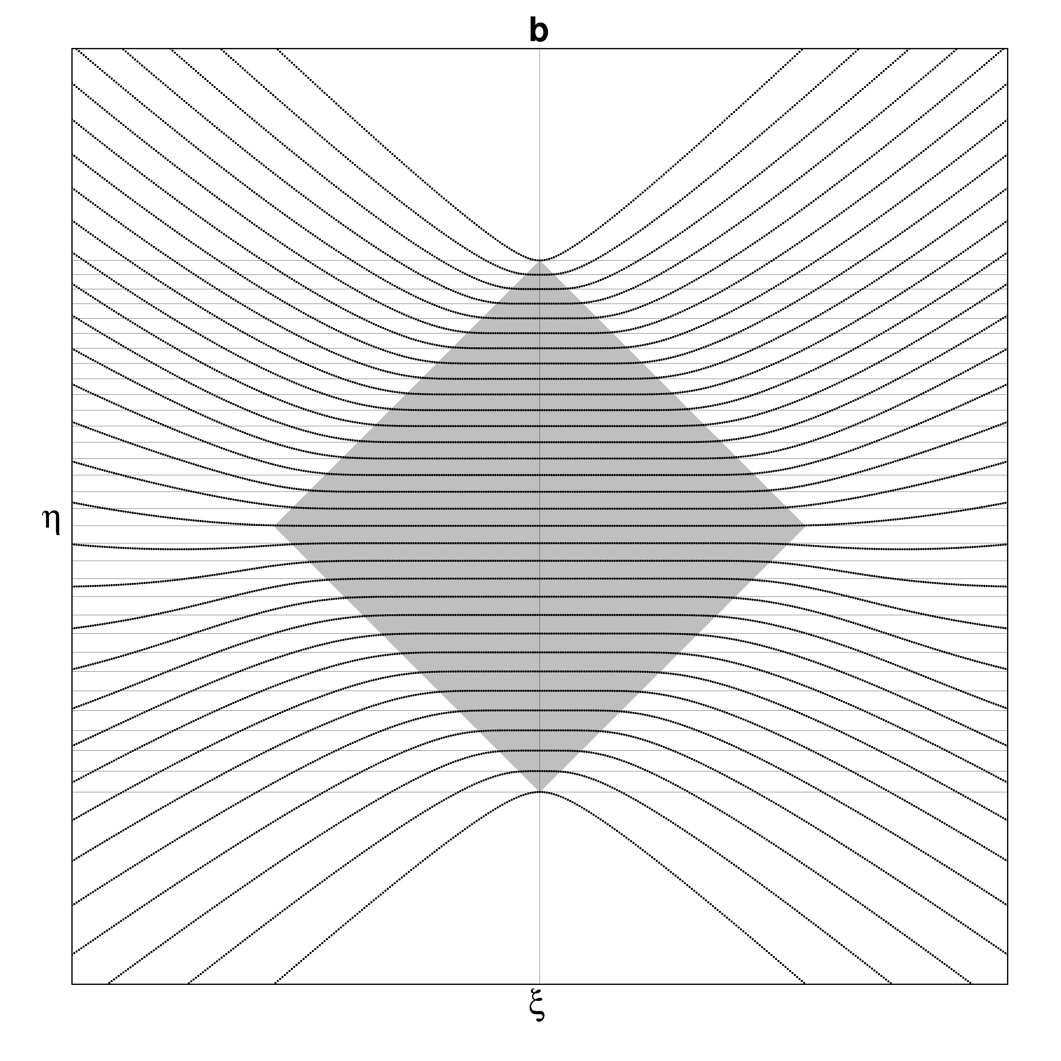
Figure 5.2: Dependence of numerically found energy levels of harmonic oscillator (5.8) on the auxiliary basis frequency $\omega$ for $k_{1}=2$, $k_{2}=60$ (a) and $k_{1}=130$, $k_{2}=190$ (b): points represent the numerical data, solid lines are exact energy levels and gray color fills the stability region determined from semiclassical analysis (5.12)

Obviously the optimal basis will be that which corresponds to maximum vertical dimensions of the stability region. In the considered example it evidently corresponds to frequency $\omega=1$.

An even simpler basis set can be built on plane waves — eigenfunctions of one-dimensional billiard, i.e. infinitely deep potential well with walls in the points $x_{1,2}=\pm a$:

$$\varphi_{k}(x;a)=\left\{\begin{array}[]{cc}\frac{1}{\sqrt{a}}\sin\frac{\pi k}{2a}(x+a),&|x|\leq a\\ 0,&|x|>a\end{array}\right..$$ (5.13)

The semiclassical phase space localization analysis can be applied to the basis functions (5.13) as well, if we take into account that they are localized on the straight lines

$$\left\{\begin{array}[]{l}x=\pm a\\ p=\pm\frac{\pi\hbar}{2a}k\end{array}\right..$$

We should note that, unlike the harmonic oscillator, the plane waves basis (5.13) cannot be cut from below: $k_{1}=1$. As result the stability region on the $(E,a)$-diagram for computation of the harmonic oscillator spectrum (5.9) in the plain waves basis (5.13) with indexes $k=1,\ldots,k_{2}$ is represented by the interior of a curvilinear triangle with base $E=0$ and bordered by a parabola and a quadratic hyperbola, depending on $k_{2}$:

$$\left\{\begin{array}[]{l}E_{n}<\frac{a^{2}}{2}\\ E_{n}<\frac{\pi^{2}\hbar^{2}}{8a^{2}}k_{2}^{2}\end{array}\right..$$

In the variables

$$\left(\eta=\log_{2}E,\ \xi=\log_{2}a,\ \nu=\log_{2}\pi\hbar k_{2}\right)$$

the computational stability region takes the form of a normal triangle (see fig.5.3a)

$$\left\{\begin{array}[]{l}\eta<2\xi-1\\ \eta<2(\nu-\xi)-3\end{array}\right..$$ (5.14)

The vertex of the triangle (5.14)

$$\left(\xi=\frac{\nu-1}{2},\eta=\nu-2\right)$$

corresponds to the optimal basis with parameter

$$a=\sqrt{\frac{\pi\hbar k_{2}}{2}},$$ (5.15)

which allows correct calculation of energy levels up to

$$E_{max}=\frac{\pi\hbar}{4}k_{2}.$$

Therefore the plane waves basis (5.13) with indexes $k=1,\ldots,k_{2}$ allows the correct calculation of the harmonic oscillator energy levels (5.9) with indices $n=0,\ldots,k_{2}=N$ (see Fig.5.3b), where

$$N=\frac{\pi}{4}k_{2}-\frac{1}{2}.$$

For large basis dimensions the fraction of correctly calculated energy levels tends to the limit

$$\lim_{k_{2}\rightarrow\infty}\frac{N}{k}=\frac{\pi}{4}=75\%$$ (5.16)

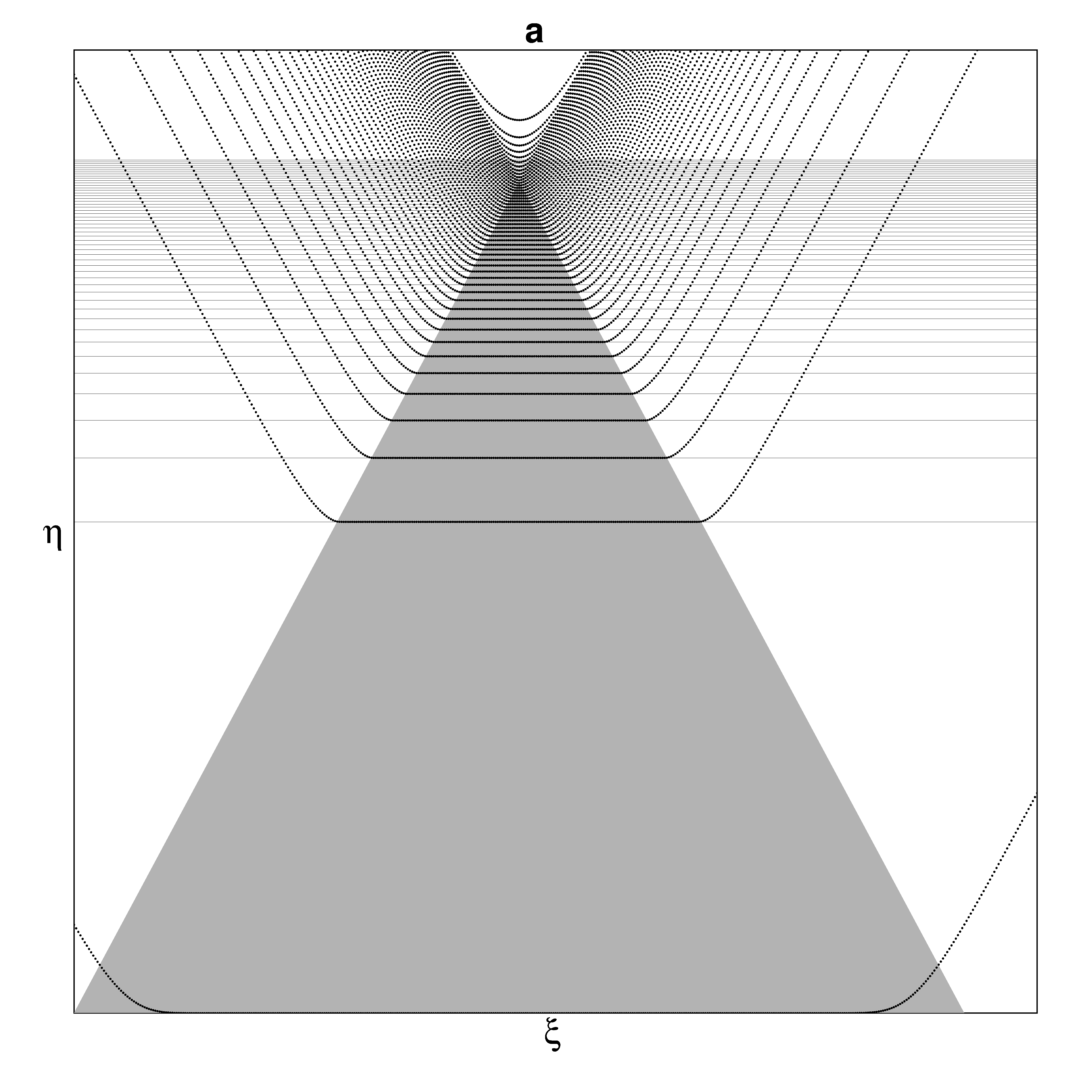
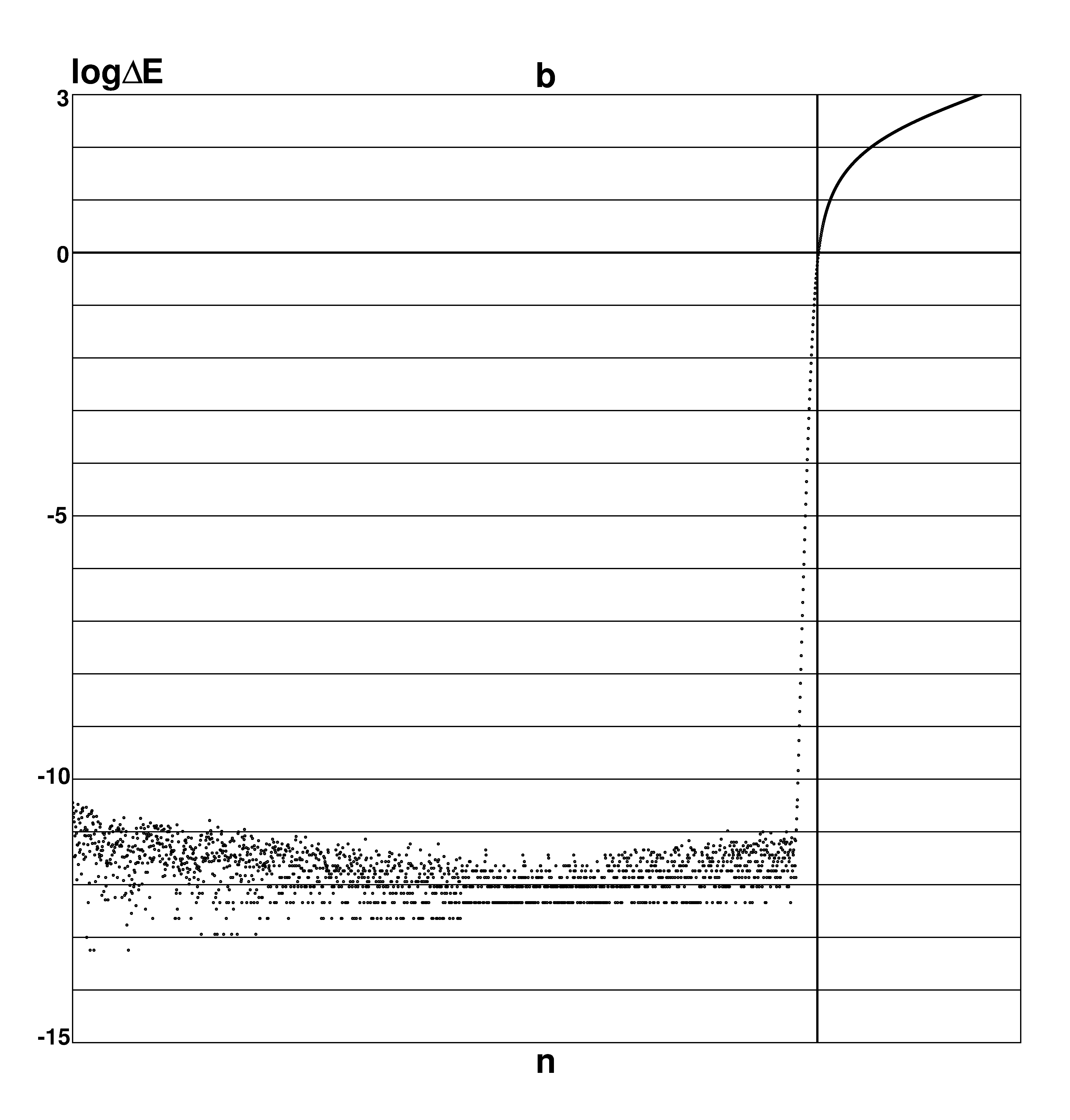
Figure 5.3: Calculation of the harmonic oscillator energy levels (5.9) in the plane waves basis (5.13) for $k_{1}=1$, $k_{2}=2500$ . a) Dependence of numerically found energy levels of harmonic oscillator (5.8) on the auxiliary basis parameter $a$: points represent the numerical data, solid lines are exact energy levels and gray color fills the stability region determined from the semiclassical analysis (5.14) b) Dependence of absolute error on main quantum number $n$ for optimal basis parameter (5.15). The vertical line corresponds to the applicability limit (5.16) of the matrix diagonalization method.

5.1.3 Quartic oscillator in 1D and in 2D

As a more complicated example let us consider calculation of energy levels for the quartic oscillator

$$H(p,x)=x^{2}+p^{4}.$$ (5.17)

As distinct from the harmonic oscillator, this quantum mechanical problem does not allow analytical solution, but there is a very accurate semiclassical approximation for the quartic oscillator spectrum [82]

$$\begin{array}[]{c}E_{n}\approx\pi^{2}\left(\frac{3\sqrt{2}\left(n+\frac{1}{2}\right)}{\Gamma\left(\frac{1}{4}\right)}\right)^{\frac{4}{3}}\left\{1+\frac{1}{9\pi\left(n+\frac{1}{2}\right)^{2}}\right.\\ \left.-\frac{\frac{5}{8}+\frac{11}{6}\left(\frac{\Gamma\left(\frac{1}{4}\right)^{2}}{4\pi}\right)^{4}}{\left[9\pi\left(n+\frac{1}{2}\right)^{2}\right]^{2}}+\frac{\frac{11}{12}+\frac{341}{10}\left(\frac{\Gamma\left(\frac{1}{4}\right)^{2}}{4\pi}\right)^{4}}{\left[9\pi\left(n+\frac{1}{2}\right)^{2}\right]^{3}}+\ldots\right\}\end{array},$$ (5.18)

Formula (5.18) gives the energy levels with $15$ correct digits, which is quite sufficient to check the numerical results in the given case. The results of such a check are presented on Fig.5.4 for the plane waves basis (5.13) and on Fig.5.5 for the harmonic oscillator basis (5.10).

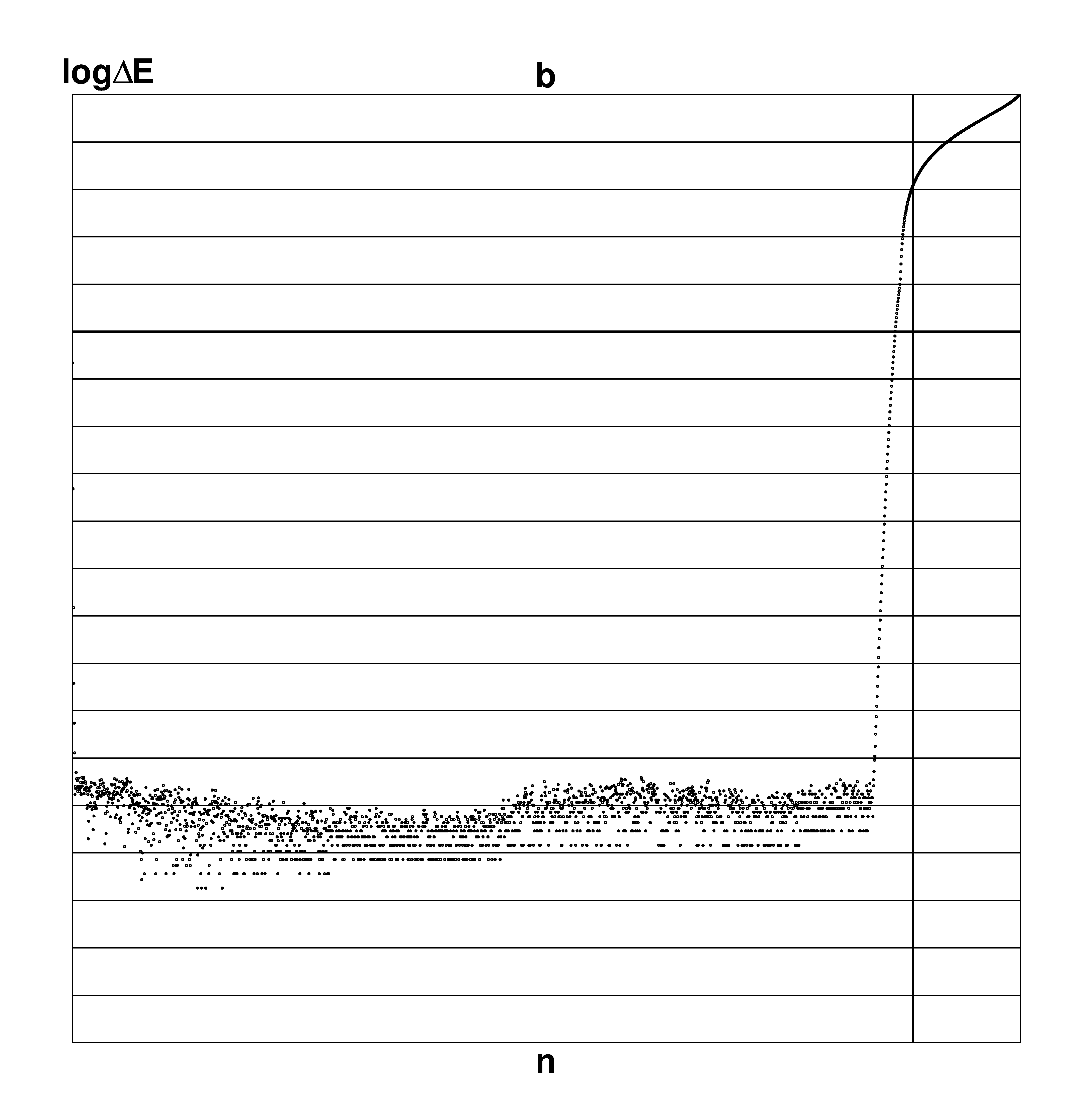
Figure 5.4: Calculation of energy levels of quartic oscillator (5.17) in the plane waves basis (5.13) for $k_{1}=2$, $k_{2}=2500$. a) Dependence of numerically found energy levels on the auxiliary basis parameter $a$: points represent the numerical data, solid lines are exact energy levels and gray color fills the stability region determined from the semiclassical analysis b) Dependence of absolute errors on main quantum number $n$ for optimal basis parameter. The vertical line corresponds to the applicability limit of the matrix diagonalization method.

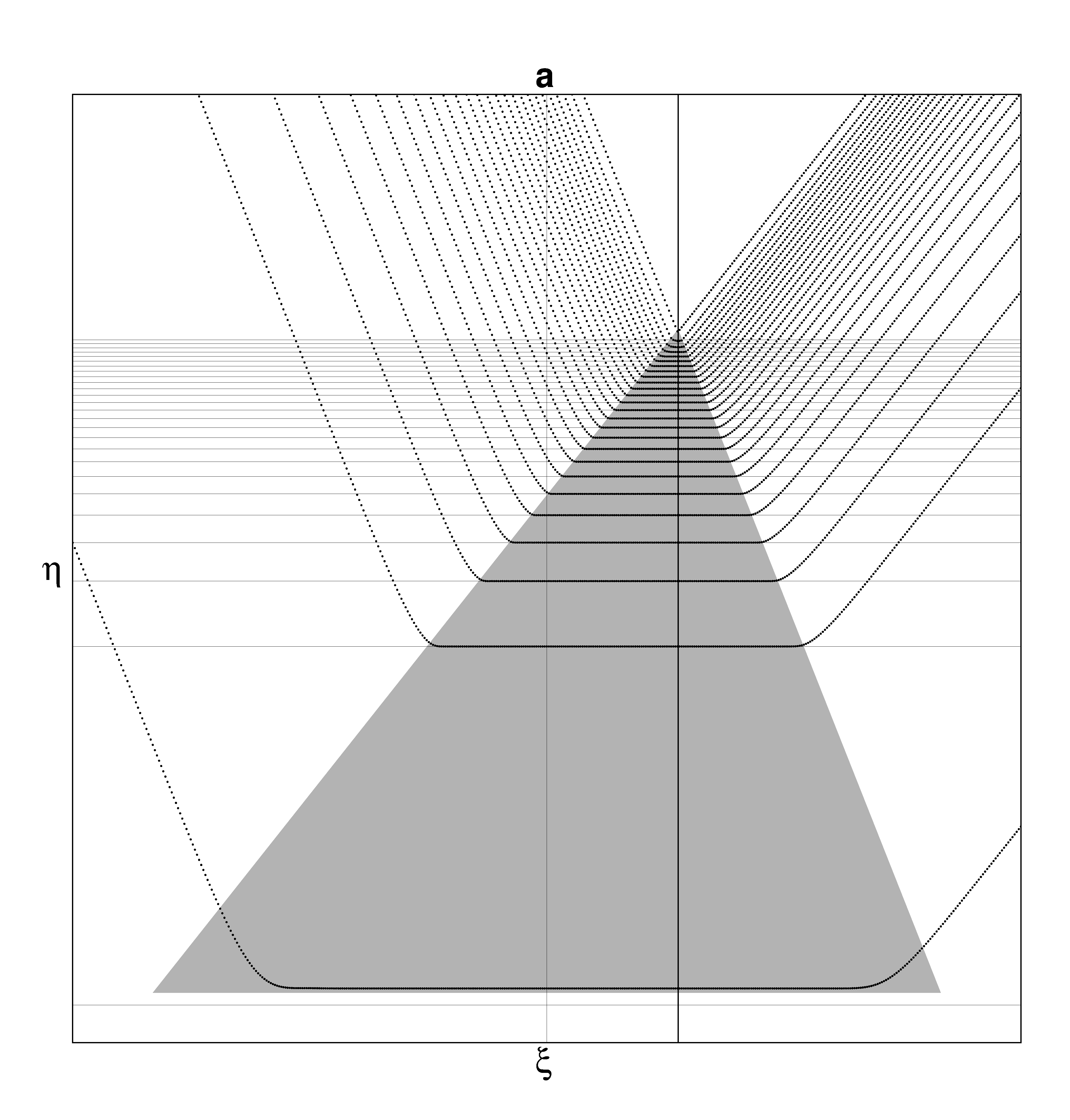
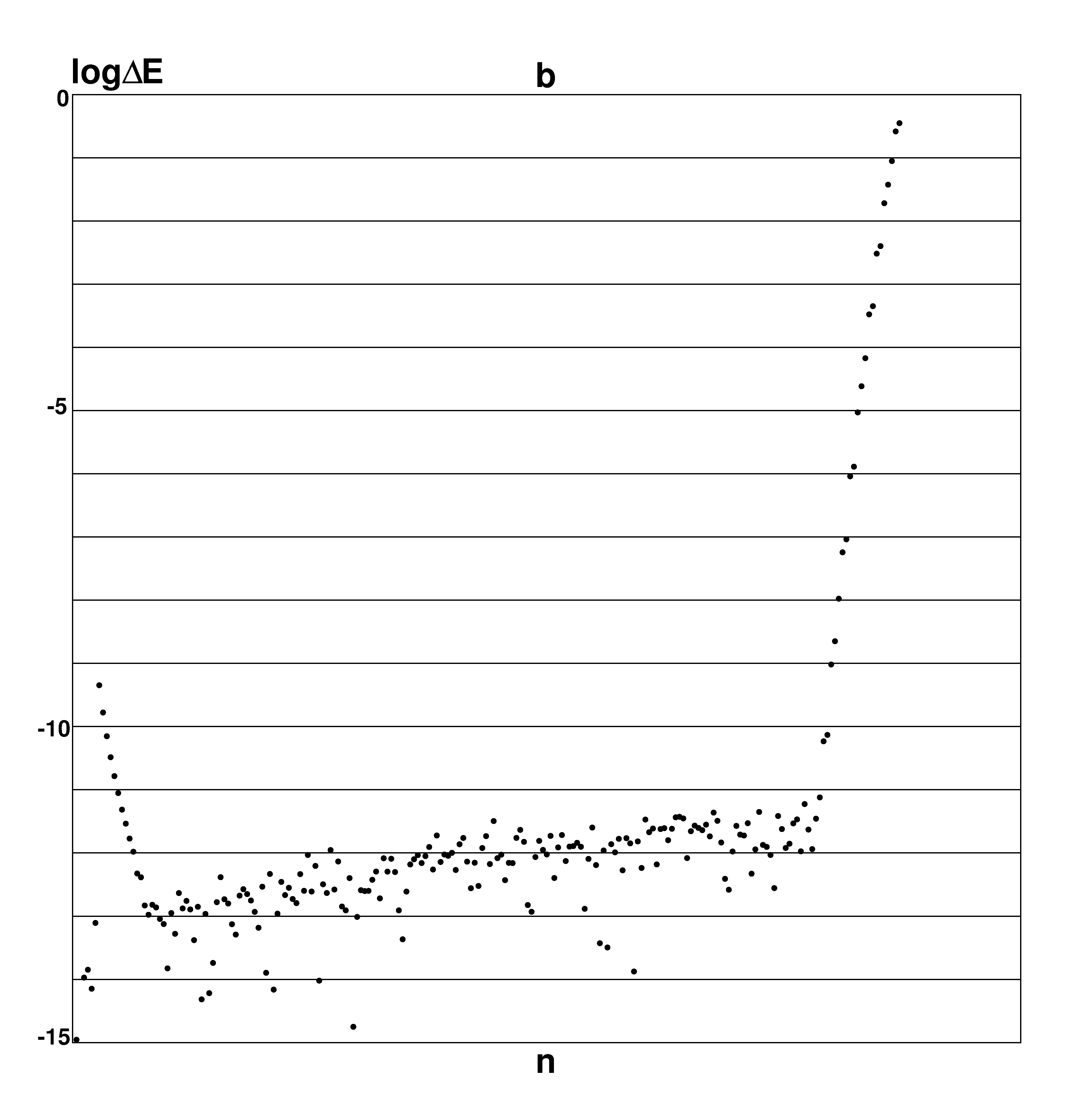
Figure 5.5: Calculation of energy levels of quartic oscillator (5.17) in the harmonic oscillator basis (5.10) for $k_{1}=2$, $k_{2}=250$. (a) Dependence of numerically found energy levels on the auxiliary basis frequency $\omega$: points represent the numerical data, solid lines are exact energy levels and gray color fills the stability region determined from the semiclassical analysis b) Dependence of absolute errors on main quantum number $n$ for optimal basis parameter.

Semiclassical phase space analysis gives the following results for the quartic oscillator (5.17): the stability region is determined by the conditions

$$\left\{\begin{array}[]{c}E_{n}<a^{4}\\ E_{n}<\frac{\pi^{2}\hbar^{2}}{4a^{2}}k_{2}^{2}\end{array}\right.$$

for the plane waves basis (5.13) and

$$\left\{\begin{array}[]{c}E_{n}<2\hbar\omega\left(k+\frac{1}{2}\right)-\frac{\omega^{4}}{4}\\ E_{n}<\frac{4\hbar^{2}}{\omega^{2}}\left(k+\frac{1}{2}\right)^{2}\end{array}\right.$$

in the harmonic oscillator basis (5.10). Now it is easy to obtain expressions for optimal basis parameters and maximum energies of correctly calculable states:

$$\begin{array}[]{cc}a=\left(\frac{\pi\hbar k}{2}\right)^{\frac{1}{3}},&E_{max}^{PW}=\left(\frac{\pi\hbar k}{2}\right)^{\frac{4}{3}}\\ \omega=\left[2\hbar\left(k+\frac{1}{2}\right)\right]^{\frac{1}{3}},&E_{max}^{HO}=\frac{3}{4}\left[2\hbar\left(k+\frac{1}{2}\right)\right]^{\frac{4}{3}}.\end{array}$$

Taking into account (5.18), we obtain for the relative number of correctly calculated energy levels

$$\frac{N}{k_{2}}\approx\frac{\Gamma^{2}\left(\frac{1}{4}\right)}{6\sqrt{2\pi}}\approx 0.874$$

for the plane waves basis (5.13) and

$$\frac{N}{k_{2}}\approx\frac{\Gamma^{2}\left(\frac{1}{4}\right)}{2\pi^{\frac{3}{2}}3^{\frac{1}{4}}}\approx 0.897$$

in the harmonic oscillator basis (5.10). Hence it follows that the latter is slightly more efficient.

Harmonic oscillator (5.10) and infinitely deep potential well (5.13) in fact exhaust the set of exactly solvable one-dimensional quantum systems whose eigenfunctions can be used as a basis for matrix diagonalization. There are many more possibilities in the models with dimensionality of more then one. Further, for simplicity we consider only two-dimensional systems, but the results can be trivially generalized for higher dimensions.

The simplest type of two-dimensional basis can be constructed from products of eigenfunctions of exactly solvable one-dimensional problems, for example, from plane waves

$$\varphi_{k_{x},k_{y}}(x,y;a_{x},a_{y})=\frac{1}{\sqrt{a_{x}a_{y}}}\sin{\frac{\pi k_{x}}{2a_{x}}(x+a_{x})}\sin{\frac{\pi k_{y}}{2a_{y}}(x+a_{y})},$$ (5.19)

harmonic oscillator eigenfunctions

$$\varphi_{k_{x},k_{y}}(x,y;\omega_{x},\omega_{y})=\frac{\left(\omega_{x}\omega_{y}\right)^{\frac{1}{4}}}{\sqrt{\pi\hbar}}\frac{H_{k_{x}}(\sqrt{\frac{\omega_{x}}{\hbar}}x)H_{k_{y}}(\sqrt{\frac{\omega_{y}}{\hbar}}y)}{\sqrt{2^{k_{x}+k_{y}}k_{x}!k_{y}!}}e^{-(\omega_{x}x^{2}+\omega_{y}y^{2})/(2\hbar)},$$ (5.20)

or as a combination of both of them

$$\varphi_{k_{x},k_{y}}(x,y;a,\omega)=\frac{1}{\sqrt{a}}\left(\frac{\omega}{\pi\hbar}\right)^{\frac{1}{4}}\sin{\frac{\pi k_{x}}{2a}(x+a)}\frac{H_{k_{y}}(\sqrt{\frac{\omega}{\hbar}}y)}{\sqrt{2^{k_{y}}k_{y}!}}e^{-\frac{\omega y^{2}}{2\hbar}}$$ (5.21)

Efficiency of the basis types (5.19,5.20,5.21) depends on the problem under consideration, but in any case simple semiclassical phase space analysis allows us to choose the most preferable among them. Skipping cumbersome exact expressions, let us give only the ultimate results (Fig.5.6,5.7a) of the semiclassical optimization of the spectrum calculation in the two-dimensional potential of coupled quartic oscillators (CQO)

$$U_{4}(x,y;\alpha)=x^{4}+y^{4}+\alpha x^{2}y^{2}.$$ (5.22)

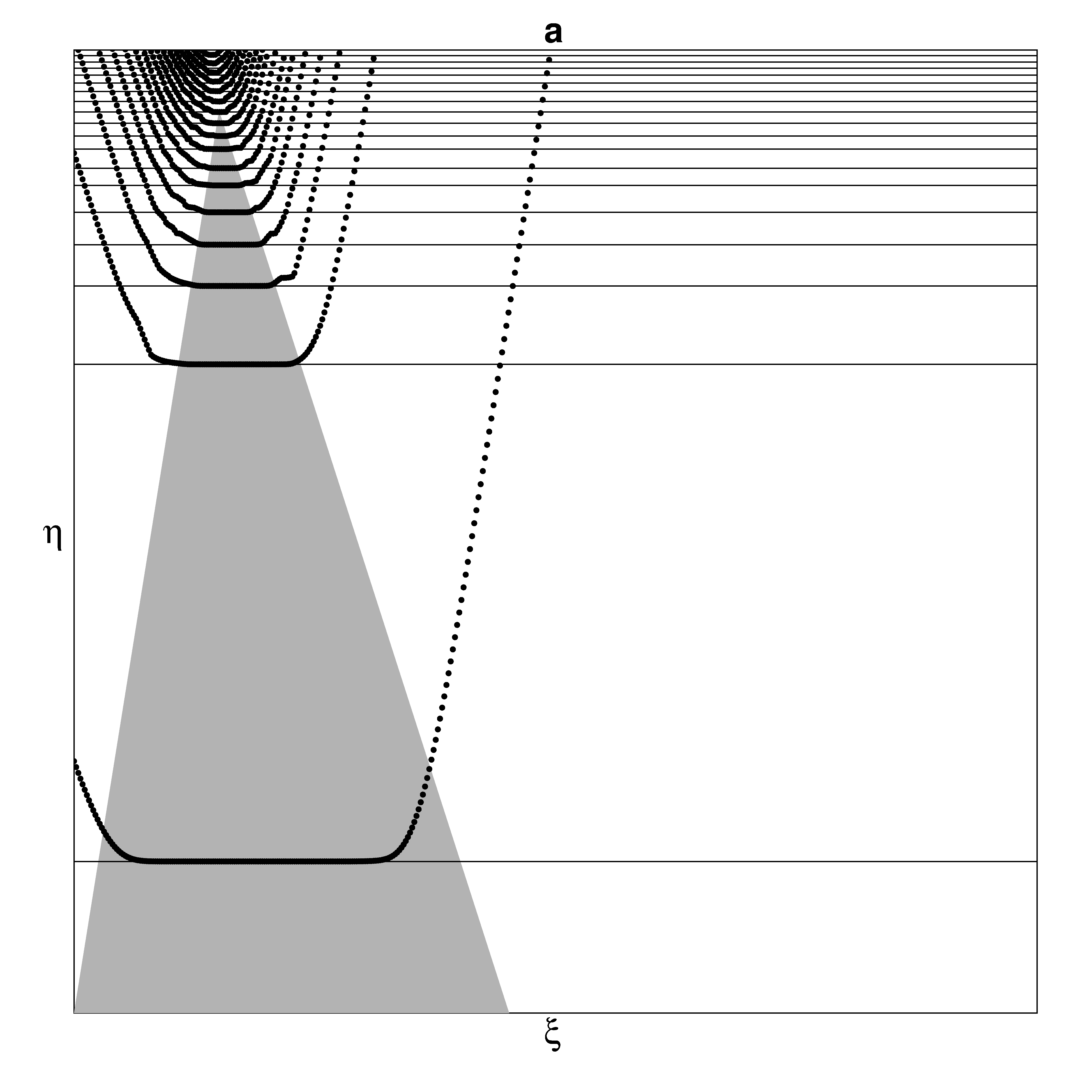
Figure 5.6: Calculation of energy levels of CQO potential (5.22) with $\alpha=6$ in the harmonic oscillator basis (5.20). a) Dependence of numerically found energy levels on the auxiliary basis frequency $\omega=\omega_{x}=\omega_{y}$: points represent the numerical data, solid lines are exact energy levels and gray color fills the stability region determined from the semiclassical analysis b) Dependence of absolute errors on main quantum number $n$ for optimal basis parameter.

Quite often the Hamiltonian of the system under consideration has a discrete symmetry. For example, the CQO potential (5.22) is invariant under transformations of square symmetry group $C_{4v}$. In such cases it is convenient for many reasons to calculate the states of different symmetry types independently. Firstly, for investigation of statistical properties of energy spectra in quantum chaology we have anyway to exclude pure spectral series — sequences of states with one and the same symmetry type. Secondly, as a rule, states of different symmetry, even and odd for example, are usually very close in energy if not degenerate. Therefore numerical computation of all symmetry types of states together leads to very ill-conditioned matrices, while exclusion of certain symmetry type improves the conditionality. And lastly, computation of different symmetry types one-by-one runs evidently faster than determination of all the states altogether. For example, the basis for determination of $A_{1}$-type states in the CQO potential (5.22) is constructed from symmetrized combinations of the form $\varphi_{mn}+\varphi_{nm}$ of basis vectors (5.19) with $a_{x}=a_{y}$, ($m,n$ odd) or (5.20) with $\omega_{x}=\omega_{y}$ ($m,n$ even).

The characteristic feature of polynomial potential is the sparse band structure of the Hamiltonian matrix (Fig.5.7b) in the basis of harmonic oscillator (5.20). For example, for large basis dimensions $n$ the bandwidth for $A_{1}$-type states in the CQO potential (5.22) is equal $m\approx 2\sqrt{2n}$. Clearly for polynomial potentials it makes sense to use special routines for band matrix diagonalization which allows us to economize both the CPU time and memory usage for computations.

Simple analysis shows that the number of non-zero matrix elements for $A_{1}$-type states in the CQO potential (5.22) never exceeds $11n$. It means that the used basis vectors ordering is not optimal and that there possibly exists another ordering which leads to band matrices with constant bandwidth $m=5$, or at least with slower growing bandwidth. Such ideal ordering would considerably speed up the computations but its search represents a non-trivial task.

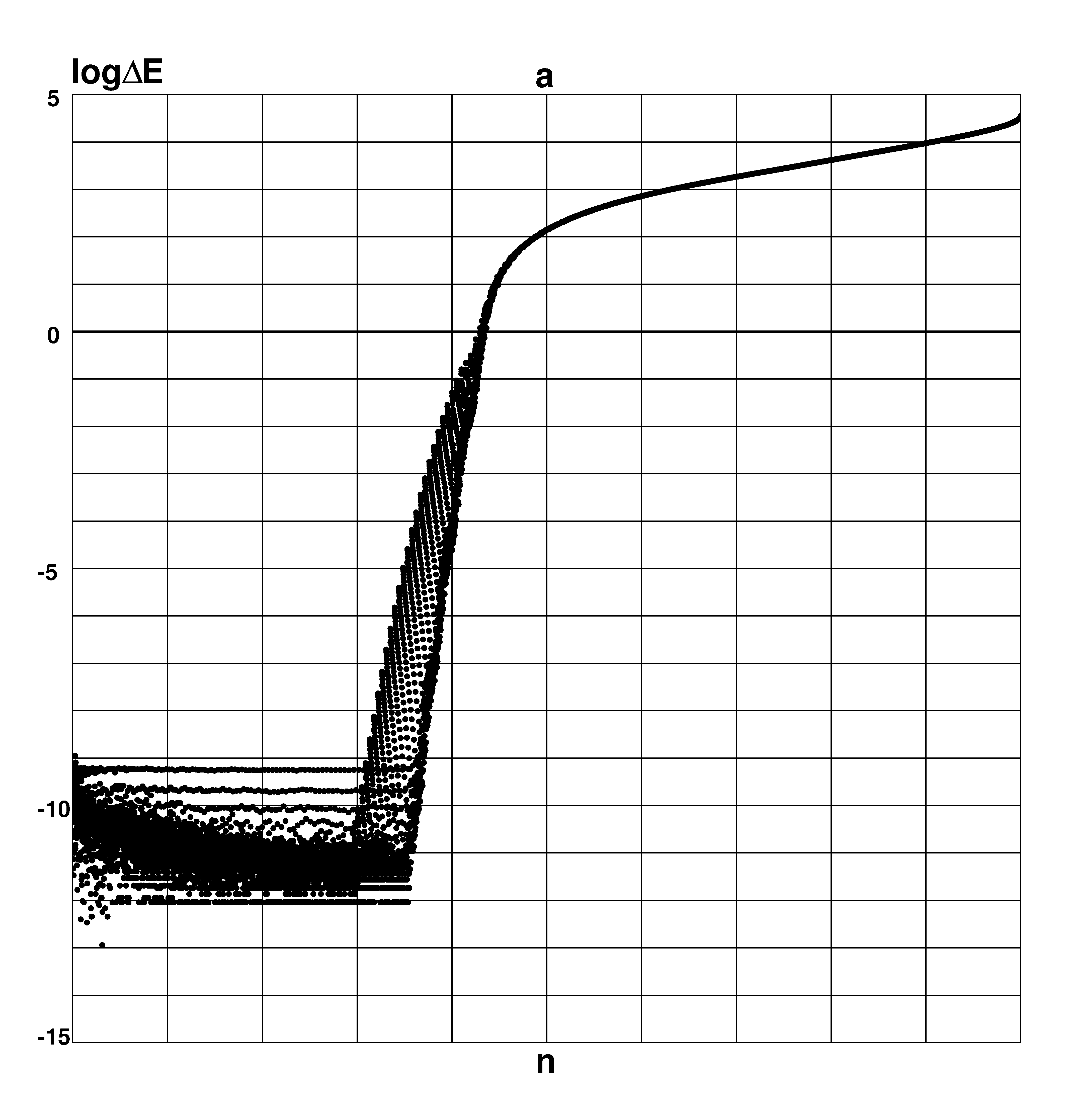
Figure 5.7: a) Comparison of numerically found energy levels of CQO potential (5.22) with $\alpha=6$ in the plane waves basis (5.19) and in the harmonic oscillator basis (5.20) for optimal parameter of both bases. b) Distribution of non-zero Hamiltonian matrix elements in the harmonic oscillator basis (5.20) for $A_{1}$-type states in the CQO potential (5.22).

5.2 The Spectral Method

The spectral method (SM) for the solution of the Schrödinger equation was proposed in the paper [44] in application to 1D and 2D potential systems, but it can be easily generalized for the Schrödinger equations of arbitrary dimensions:

$$\left[-\frac{\hbar^{2}}{2}\sum\limits_{i=1}^{D}\partial_{i}^{2}+U(x_{1},\dots,x_{D})\right]\psi_{n}(x_{1},\dots,x_{D})=E_{n}\psi_{n}(x_{1},\dots,x_{D}),$$

where $D$ is the dimensionality of the system configuration space. Let us assume that the potential $U(x_{1},\dots,x_{D})$ allows only finite motion for all energies, therefore our task is to find discrete energy spectrum $E_{n}$ and stationary wave functions $\psi_{n}(x_{1},\dots,x_{D})$.

Let us consider time-dependent solution $\psi(x_{1},\dots,x_{D};t)$ for the corresponding non-stationary Schrödinger equation

$$\left[-\frac{\hbar^{2}}{2}\sum\limits_{i=1}^{D}\partial_{i}^{2}+U(x_{1},\dots,x_{D})\right]\psi(x_{1},\dots,x_{D};t)=i\hbar\partial_{t}\psi(x_{1},\dots,x_{D};t)$$

with some in principle arbitrary initial condition

$$\psi_{0}(x_{1},\dots,x_{D})=\psi_{n}(x_{1},\dots,x_{D};t=0)$$

. Applying the decomposition

$$\psi_{0}(x_{1},\dots,x_{D})=\sum\limits_{n=1}^{\infty}a_{n}\psi_{n}(x_{1},\dots,x_{D}),$$

we obtain

$$\psi(x_{1},\dots,x_{D};t)=\sum\limits_{n=1}^{\infty}a_{n}\psi_{n}(x_{1},\dots,x_{D})e^{-i\frac{E_{n}t}{\hbar}}.$$

Here and further we imply that the wave functions $\psi_{n}(x_{1},\dots,x_{D})$ are orthonormal

$$\int dx_{1}\ldots dx_{D}\bar{\psi}_{i}(x_{1},\dots,x_{D})\psi_{k}(x_{1},\dots,x_{D})=\delta_{ik}.$$

Let us consider autocorrelation function of the form

$$P(t)=\int dx_{1}\ldots dx_{D}\bar{\psi}_{0}(x_{1},\dots,x_{D})\psi(x_{1},\dots,x_{D};t)=\sum\limits_{n=1}^{\infty}\left|a_{n}\right|^{2}e^{-i\frac{E_{n}t}{\hbar}}.$$ (5.23)

We assume the initial wave function $\psi_{0}(x_{1},\dots,x_{D})$ to be normalized

$$\int dx_{1}\ldots dx_{D}\bar{\psi}_{0}(x_{1},\dots,x_{D})\psi_{0}(x_{1},\dots,x_{D})=\sum\limits_{n=1}^{\infty}\left|a_{n}\right|^{2}=1,$$

so that $P(0)=1$. The Fourier transform of the autocorrelator (5.23) contains information about the energy spectrum $E_{n}$ of the system

$$P(E)=\int\limits_{-\infty}^{\infty}dte^{i\frac{Et}{\hbar}}P(t)=\hbar\sum\limits_{n=1}^{\infty}\left|a_{n}\right|^{2}\delta\left(E-E_{n}\right).$$ (5.24)

For determination of stationary wave functions $\psi_{n}(x_{1},\dots,x_{D})$ we will need the Fourier transform of $\psi(x_{1},\dots,x_{D};t)$ itself

$$\psi(x_{1},\dots,x_{D};E)=\int\limits_{-\infty}^{\infty}dte^{i\frac{Et}{\hbar}}\psi(x_{1},\dots,x_{D};t)=\hbar\sum\limits_{n=1}^{\infty}a_{n}\psi_{n}(x_{1},\dots,x_{D})\delta\left(E-E_{n}\right).$$ (5.25)

Naturally in practice we never try to find all $E_{n}$ and $\psi_{n}(x_{1},\dots,x_{D})$. Usually the task is to determine all the energy levels $E_{n}$ inside a given interval $E_{1}<E<E_{2}$ with certain accuracy $\delta_{E}$ and to calculate the corresponding stationary wave functions $\psi_{n}(x_{1},\dots,x_{D})$ on some finite set of points $\left\{x_{i}^{(k_{i})}=x_{i}^{(0)}+k_{i}\Delta x_{i},\ k_{i}=0,\ldots,N_{i}\right\}$ also with finite accuracy. Further we will assume for simplicity that all $N_{i}$ are equal.

Let us show how to apply expressions (5.24,5.25) for computation procedure construction. It is evident that in practical calculations we always deal with only a finite number of data known also with finite accuracy. In our case it means that the principal function — $\psi(x_{1},\dots,x_{D};t)$ — will be known on a finite set of points both on temporal and spacial coordinates. Accordingly the autocorrelation function (5.23) can be calculated also only on a finite set of points $t_{k}=k\Delta t,\ k=1,\ldots,M$, and therefore we have to apply the finite analogues of the Fourier transforms (5.24) and (5.25)

$$P_{T}(E)=\frac{1}{T}\int\limits_{0}^{T}dte^{i\frac{Et}{\hbar}}P(t)=\hbar\sum\limits_{n=1}^{\infty}\left|a_{n}\right|^{2}\delta_{T}\left(E-E_{n}\right)$$ (5.26)

$$\begin{array}[]{c}\psi_{T}(x_{1},\dots,x_{D};E)=\frac{1}{T}\int\limits_{0}^{T}dte^{i\frac{Et}{\hbar}}\psi(x_{1},\dots,x_{D};t)\\ =\hbar\sum\limits_{n=1}^{\infty}a_{n}\psi_{n}(x_{1},\dots,x_{D})\delta_{T}\left(E-E_{n}\right),\end{array}$$ (5.27)

where $T=M\Delta t$ and the finite analogue of $\delta$-function takes the form

$$\begin{array}[]{c}\delta_{T}(E)=\frac{1}{T}\int\limits_{0}^{T}dte^{i\frac{Et}{\hbar}}=\frac{e^{i\frac{ET}{\hbar}}-1}{i\frac{ET}{\hbar}}=f_{T}\left(i\frac{ET}{h}\right)\\ f_{T}(x)=\frac{\sin\pi x}{\pi x}e^{i\pi x}.\end{array}$$

As distinct from the usual $\delta$-function, $\delta_{T}(0)=1$ (see Fig.5.8a).

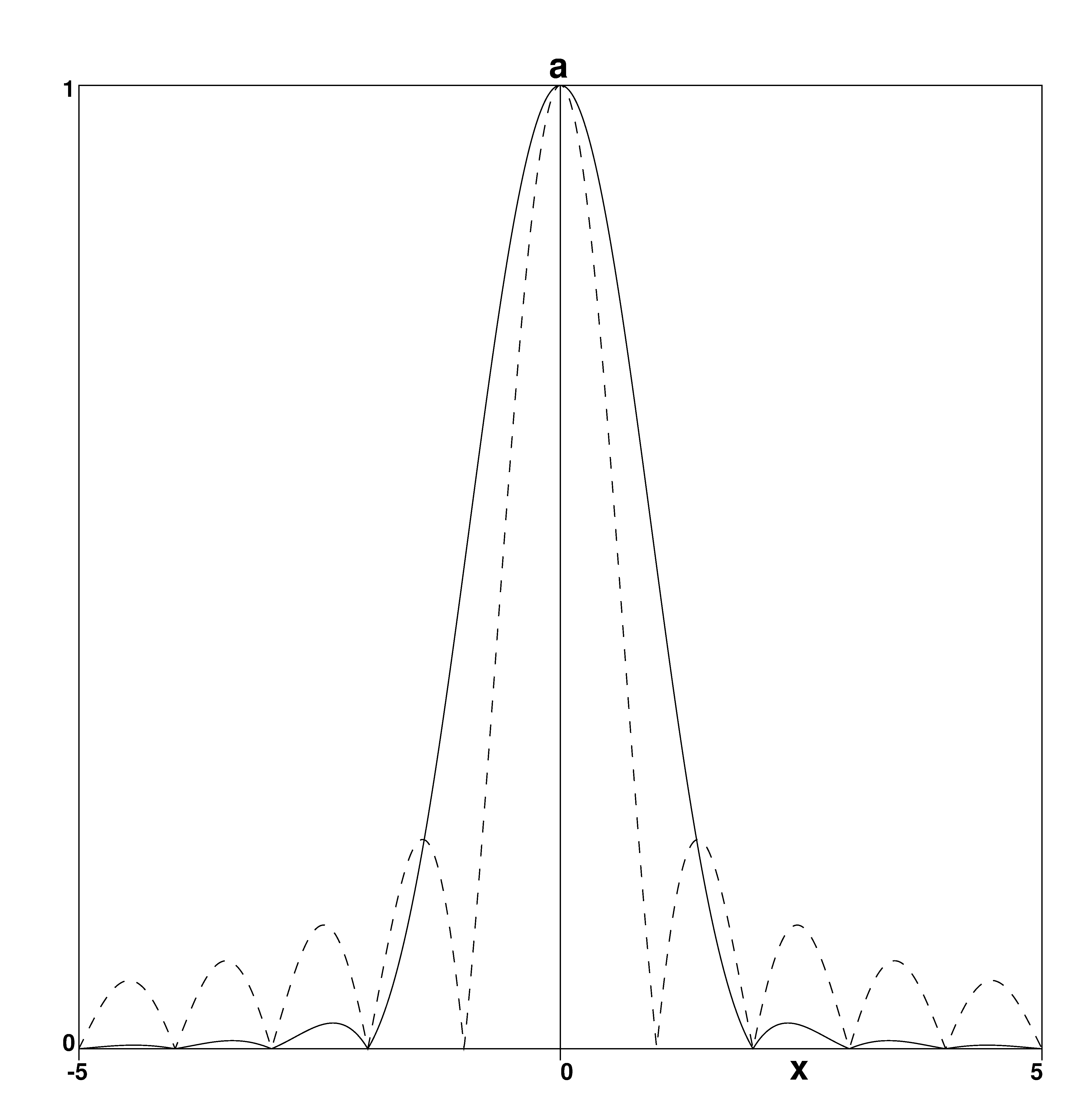
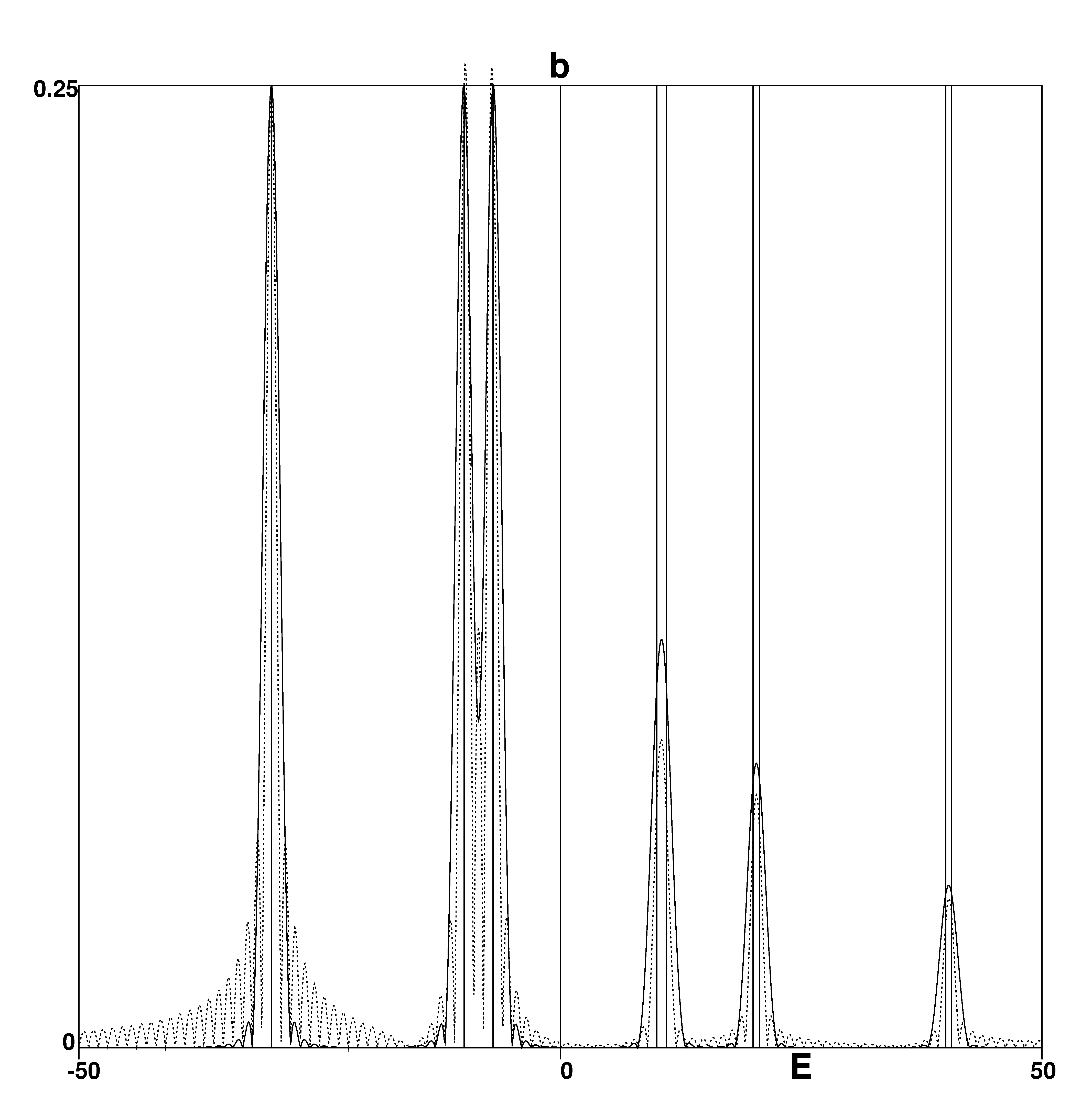
Figure 5.8: a) $\left|f_{T}(x)\right|$ profile (dashed line) and $\left|f_{H}(x)\right|$ profile (solid line). b) $\left|P_{T}(E)\right|$ (dashed line) and $\left|P_{H}(E)\right|$ (solid line) for the model system with energy spectrum $E_{1,2,\ldots,9}=\{-30,-10,-7,10,11,20,20.7,40,40.63\}$ (marked by solid vertical lines) and $a_{1,2,\ldots,9}=\{0.5,0.5,0.5,0.25,0.25,0.2,0.2,0.15,0.15\}$ with $h=T=1$.

Therefore each energy level $E_{n}$ corresponds to a sufficiently sharp peak — local maximum of the function $|P_{T}(E)|$, situated at the point $E=E_{n}$ (Fig. 5.8b). The typical profile of the function $|P_{T}(E)|$ has many local maxima (Fig.5.9), but a major part of them has absolutely nothing to do with the energy levels of the system under consideration — they appear due to the oscillating character of $\delta_{T}(E)$. So the full number of maxima on Fig.5.8b equals $94$, while the corresponding system has only $9$ physical energy levels in reality. Therefore, formally analyzing $|P_{T}(E)|$, we will obtain plenty of extra ”parasite levels”. The unique characteristic that allows us to distinguish such phantom levels from the real ones is the relative smallness of $|P_{T}(E)|$ in corresponding local maxima. However if we were just to ignore all the levels that have $|P_{T}(E)|$ peak amplitude less than a certain fixed threshold value, we risk loosing some real physical levels, which correspond to small values of $|a_{n}|$. In this connection it is very useful to apply the weighted Fourier transform:

$$\begin{array}[]{c}P_{w}(E)=\frac{1}{T}\int\limits_{0}^{T}dte^{i\frac{Et}{\hbar}}P(t)w(t)=\sum\limits_{n=1}^{\infty}\left|a_{n}\right|^{2}\delta_{w}\left(E-E_{n}\right)\\ \psi_{w}(x_{1},\ldots,x_{D};E)=\frac{1}{T}\int\limits_{0}^{T}dte^{i\frac{Et}{\hbar}}\psi(x_{1},\ldots,x_{D};t)w(t)=\\ =\sum\limits_{n=1}^{\infty}a_{n}\psi_{n}(x_{1},\ldots,x_{D})\delta_{w}\left(E-E_{n}\right)\\ \delta_{w}(E)=\frac{1}{T}\int\limits_{0}^{T}dte^{i\frac{Et}{\hbar}}w(t)\end{array}$$ (5.28)

where the weight function $w(t)$ satisfies the conditions

$$\begin{array}[]{c}w(0)=w(T)\\ \int\limits_{0}^{T}w(t)dt=1.\end{array}$$ (5.29)

Figure 5.9: $\left|P_{T}(E)\right|$ for calculation of $E$-type energy levels in the quadrupole oscillation potential.

Therefore $\delta_{w}(0)=1$ for any such $w(t)$. The simplest function, satisfying the conditions (5.29), is Hann function

$$w_{H}(t)=1-\cos\frac{2\pi t}{T},$$

for which

$$\begin{array}[]{c}\delta_{H}(E)=\frac{e^{i\frac{Et}{\hbar}}-1}{i\frac{Et}{\hbar}}-\frac{1}{2}\left[\frac{e^{i\left(\frac{Et}{\hbar}+2\pi\right)}-1}{i\frac{Et}{\hbar}+2\pi}+\frac{e^{i\left(\frac{Et}{\hbar}-2\pi\right)}-1}{i\frac{Et}{\hbar}-2\pi}\right]=f_{H}\left(\frac{Et}{h}\right)\\ f_{H}(x)=\frac{\sin(\pi x)e^{i\pi x}}{\pi x(1-x^{2})}=\frac{f_{T}(x)}{1-x^{2}}.\end{array}$$

Inclusion of the weight function in the modified Fourier transform allows us to diminish the relative amplitude of the phantom peaks in $|P_{H}(E)|$ (Fig.5.8a) and even slightly decrease their number — to $76$ for $|P_{H}(E)|$ instead of $86$ for $|P_{T}(E)|$ (Fig.5.8b). Numerical analysis of the $|f_{T}(x)|$ shape shows that the second maximum is situated in points $x_{Tmax}\approx\pm 1.43$ and has amplitude $f_{Tmax}\approx 0.217$, while for the $|f_{H}(x)|$ the analogous analysis maximum is situated almost twice farther from the principal one — $x_{Hmax}\approx\pm 2.36$, and its amplitude appears less for whole order of magnitude — $f_{Tmax}\approx 0.0267$. Amplitude of more distant maxima decrease even faster (Fig.5.8a).

Besides that, an important independent criterion to estimate the accuracy of numerical results can be realized using the semiclassical approximation for the stair-case states number function $n(E)$: comparison of numerical $n(E)$ with the semiclassical one allows us to roughly estimate the number of lost or acquired extra levels (fig.5.10).

Figure 5.10: State number $n(E)$ (dashed line) in Thomas-Fermi approximation versus the numerically obtained $n(E)$ (solid line) for lower umbilic catastrophe $D_{5}$ potential.

Analyzing the positions and amplitudes of the $\left|P_{H}(E)\right|$ local maxima one can determine the energy levels $E_{n}$ and absolute magnitudes of the coefficients $a_{n}$

$$\left|a_{n}\right|=\sqrt{\left|P_{H}(E_{n})\right|}.$$

If in the expression

$$\psi_{H}(x_{1},\ldots,x_{D};E_{n})=a_{n}\psi_{n}(x_{1},\ldots,x_{D})+\sum\limits_{k\neq n}a_{k}\psi_{k}(x_{1},\ldots,x_{D})\delta_{H}(E_{n}-E_{k})$$

we now neglect the terms containing $\delta_{H}(E_{n}-E_{k})$ (compare with 5.28), we can determine the eigenfunctions up to a phase factor:

$$\psi_{n}(x_{1},\ldots,x_{D})\approx\frac{1}{\left|a_{n}\right|}\psi_{H}(x_{1},\ldots,x_{D};E_{n})$$ (5.30)

Here and forth we consider that there are no degenerate levels among $E_{n}$. In practice in any system with a degenerate spectrum we can (and should) remove the degeneracy by a certain choice of the initial state $\psi_{0}(x_{1},\ldots,x_{D})$.

However such an approach is applicable only while the given energy level $E_{n}$ is sufficiently separated from the neighbors. Indeed, if one or more levels are situated at too short a distance, the position of corresponding maxima $\left|P_{H}(E_{n})\right|$ considerably differs from the actual values $E_{n}$. Moreover for sufficiently close levels the $\left|P_{H}(E_{n})\right|$ profile will have only a single common peak (Fig.5.8b).

In general, it looks impossible to determine exactly the minimum separation between close levels at which they still can be resolved, but we can state with confidence that this value is of the order of $\Delta E_{min}=h/T$ — the natural width of level. Therefore all duplets and multiplets with separation less than $\Delta E_{min}$ will give only single local maxima, and some real levels will be lost in the computed spectrum (see Table 5.1).

	$E_{1}$	$|a_{1}|$	$E_{2}$	$|a_{2}|$	$E_{3}$	$|a_{3}|$
Exact	-30.00	0.50	-10.00	0.50	-7.00	0.50
From $\left|P_{T}(E)\right|$	-30.03	0.50	-10.09	0.50	-6.91	0.50
From $\left|P_{H}(E)\right|$	-30.00	0.50	-9.97	0.50	-7.03	0.50
	$E_{4}$	$|a_{4}|$	$E_{5}$	$|a_{5}|$	$E_{6}$	$|a_{6}|$
Exact	10.00	0.25	11.00	0.25	20.00	0.20
From $\left|P_{T}(E)\right|$	9.89	0.25	11.24	0.27	20.22	0.19
From $\left|P_{H}(E)\right|$	9.53	0.21	11.47	0.21	20.35	0.18
	$E_{7}$	$|a_{7}|$	$E_{8}$	$|a_{8}|$	$E_{9}$	$|a_{9}|$
Exact	20.70	0.20	40.00	0.15	40.63	0.15
From $\left|P_{T}(E)\right|$	21.10	0.19	40.32	0.16	-	-
From $\left|P_{H}(E)\right|$	-	-	40.31	0.15	-	-

Table 5.1: Energy spectrum $E_{n}$ and eigenstates amplitudes $a_{n}$ for the model system from Fig. 5.8b

From Table 5.1 we can see that analysis of $\left|P_{H}(E)\right|$ gives considerably more accurate results for isolated levels. On the other hand, $\left|P_{T}(E)\right|$ has a smaller natural level width and gives more adequate results for close levels. However the preference of $\left|P_{T}(E)\right|$ in resolution of close levels is so insignificant that $\left|P_{H}(E)\right|$ appears more preferable in the majority of cases.

Taking into account that $P(t)$ as well as $\psi(x_{1},\ldots,x_{D};t)$ is calculated only on finite set of points $t_{k}=k\Delta t,\ k=0,\dots,M$, the most natural way to obtain $P_{H}(E)$ is the discrete Fourier transform

$$P_{H}(E_{k})=\frac{1}{M}\sum\limits_{j=0}^{M}P(t_{j})w(t_{j})e^{2\pi i\frac{jk}{M}}=\frac{\Delta t}{T}\sum\limits_{j=0}^{M}P(t_{j})w(t_{j})e^{i\frac{t_{j}E_{k}}{\hbar}},$$ (5.31)

where $E_{k}=\frac{h}{T}k,\ k=-M/2,\ldots,M/2$. Therefore $P_{H}(E)$ appears to be calculated in energy interval $-\frac{h}{2\Delta t}<E<\frac{h}{2\Delta t}$ with step $\Delta E=h/T$ exactly equal to natural level width.

As $w(T)=w(0)=0$, the discrete Fourier transform (5.31) in fact coincides with the formula for numerical integration by the trapezium rule[45], applied to (5.28), and it is easy to estimate its error

$$R_{H}(E)=\frac{T{\Delta t}^{2}}{12}\left|\frac{d^{2}}{{dt}^{2}}\left.\left(P(t)w(t)e^{i\frac{Et}{\hbar}}\right)\right|_{t=\tau}\right|$$

where $0<\tau<T$. But

$$\begin{array}[]{c}\left|\frac{d^{2}}{{dt}^{2}}\left(P(t)w(t)e^{i\frac{Et}{\hbar}}\right)\right|=\\ \left|\frac{d^{2}}{{dt}^{2}}\left[\sum\limits_{n=1}^{\infty}|a_{n}|^{2}\left(e^{2\pi i\frac{t}{h}(E-E_{n})}-\frac{1}{2}e^{2\pi i\frac{t}{h}(E-E_{n}+\frac{h}{T})}-\frac{1}{2}e^{2\pi i\frac{t}{h}(E-E_{n}-\frac{h}{T})}\right)\right]\right|\leq\\ \leq\sum\limits_{n=1}^{\infty}\frac{|a_{n}|^{2}}{\hbar^{2}}\left|(E-E_{n})^{2}-\frac{1}{2}\left(E-E_{n}+\frac{h}{T}\right)^{2}e^{2\pi i\frac{t}{T}}-\frac{1}{2}\left(E-E_{n}-\frac{h}{T}\right)^{2}e^{-2\pi i\frac{t}{T}}\right|\leq\\ \leq\frac{1}{\hbar^{2}}\sum\limits_{n=1}^{\infty}|a_{n}|^{2}\left[(E-E_{n})^{2}+\frac{1}{2}\left(E-E_{n}+\frac{h}{T}\right)^{2}+\frac{1}{2}\left(E-E_{n}-\frac{h}{T}\right)^{2}\right]=\\ =\sum\limits_{n=1}^{\infty}|a_{n}|^{2}\left[\frac{(E-E_{n})^{2}}{\hbar^{2}}+\left(\frac{2\pi}{T}\right)^{2}\right]=\frac{(E-\bar{E})^{2}}{\hbar^{2}}+2\left(\frac{D_{E}}{\hbar}\right)^{2}+\left(\frac{2\pi}{T}\right)^{2},\end{array}$$

where $\bar{E}$ and $D_{E}$ are respectively mean energy and dispersion in the initial state $\psi_{0}(x_{1},\ldots,x_{D})$:

$$\begin{array}[]{c}\bar{E}=\int{dx}_{1}\ldots{dx}_{D}\bar{\psi}_{0}(x_{1},\ldots,x_{D})\hat{H}\psi_{0}(x_{1},\ldots,x_{D})=\sum\limits_{n=1}^{\infty}|a_{n}|^{2}E_{n}\\ D_{E}^{2}=\int{dx}_{1}\ldots{dx}_{D}\bar{\psi}_{0}(x_{1},\ldots,x_{D})(\hat{H}-\bar{E})^{2}\psi_{0}(x_{1},\ldots,x_{D})=\sum\limits_{n=1}^{\infty}|a_{n}|^{2}(E_{n}^{2}-\bar{E}^{2})\\ \hat{H}=-\frac{\hbar^{2}}{2}\sum\limits_{i=1}^{D}\partial_{i}^{2}+U(x_{1},\ldots,x_{D}),\end{array}$$

and we finally get

$$R_{H}(E)\leq\frac{T\Delta t^{2}}{6\hbar^{2}}\left[(E-\bar{E})^{2}+D_{E}^{2}\right]+\frac{\pi^{2}\Delta t^{2}}{3T}.$$

Therefore formally integration in (5.28) allows us to calculate $P_{H}(E)$ for any energy values, but in fact applicability of such an approach is limited by the energy region

$$|E-\bar{E}|\ll\frac{\hbar^{2}}{\Delta t^{2}},$$

which is definitely not better than for (5.31). Application of the approximated integration formulae of higher orders also does not give any improvement to (5.31), because the error estimate for numerical integration of (5.28) by $n$-th order method reads

$$R^{(n)}_{H}(E)\approx\frac{T\Delta t^{n}}{n!\hbar^{n}}(E-\bar{E})^{n}$$

For calculation of $\psi(x_{1},\ldots,x_{D};t)$ at $t_{k}=k\Delta t,\ k=1,\ldots,M$ we can apply step-by-step the split operator method

$$\psi(x_{1},\ldots,x_{D};t+\Delta t)=e^{i\frac{\hbar^{2}\Delta t}{4}\sum\limits_{i=1}^{D}\partial_{i}^{2}}e^{-i\Delta tU(x_{1},\ldots,x_{D};t)}e^{i\frac{\hbar^{2}\Delta t}{4}\sum\limits_{i=1}^{D}\partial_{i}^{2}}\psi(x_{1},\ldots,x_{D};t)+O(\Delta t^{3}).$$

Action of the differential operator $e^{i\frac{\hbar^{2}\Delta t}{4}\sum\limits_{i=1}^{D}\partial_{i}^{2}}$ is also calculated with the help of the discrete Fourier transform

$$\begin{array}[]{c}e^{i\frac{\hbar^{2}\Delta t}{4}\sum\limits_{i=1}^{D}\partial_{i}^{2}}\psi(x_{1},\ldots,x_{D};t)=\\ =\sum\limits_{n_{1}=-N_{1}/2}^{N_{1}/2}\sum\limits_{n_{2}=-N_{2}/2}^{N_{2}/2}\ldots\sum\limits_{n_{D}=-N_{D}/2}^{N_{D}/2}\psi_{n_{1}n_{2}\ldots n_{D}}(t)e^{\sum\limits_{k=1}^{D}\left(2\pi i\frac{n_{k}x_{k}}{N_{k}\Delta x_{k}}-i\Delta t\left(\frac{hn_{k}}{2N_{k}\Delta x_{k}}\right)\right)}\\ \psi_{n_{1}n_{2}\ldots n_{D}}(t)=\frac{1}{\prod\limits_{k=1}^{D}N_{k}}\sum\limits_{n_{1}=-N_{1}/2}^{N_{1}/2}\sum\limits_{n_{2}=-N_{2}/2}^{N_{2}/2}\ldots\sum\limits_{n_{D}=-N_{D}/2}^{N_{D}/2}\psi(x_{1},\ldots,x_{D};t)e^{-2\pi i\sum\limits_{k=1}^{D}\frac{n_{k}x_{k}}{N_{k}\Delta x_{k}}}.\end{array}$$

With sufficiently large numbers of time steps $M$ and coordinate grid nodes $N$ the results of computations by the spectral method really do not depend on the arbitrary initial wave function $\psi_{0}(x_{1},\ldots,x_{D})$, but it is a reasonable choice of such a function that is the most powerful means for the optimization of computations by the spectral method in order to achieve sufficient accuracy of the results with minimal expenses of computational power.

It is convenient to choose the initial wave function $\psi_{0}(x_{1},\ldots,x_{D})$ as a linear combination of Gaussian wave packets of minimal uncertainty

$$\psi_{G}(x_{1},\ldots,x_{D})=e^{-\sum\limits_{i=1}^{D}\frac{(x_{i}-x_{i0})^{2}}{2\sigma_{i}^{2}}+i\frac{p_{i}(x_{i}-x_{i0})}{\hbar}}.$$ (5.32)

Combining functions of the form (5.32) with different parameters $\sigma,p_{i}$ and $x_{i0}$ it is possible to selectively excite eigenstates $\psi_{n}(x_{1},\ldots,x_{D})$ with the desired symmetry properties and lying in the desired energy interval. Its position

$$\langle E\rangle=\langle\psi_{0}(x_{1},\ldots,x_{D})|\bar{H}|\psi_{0}(x_{1},\ldots,x_{D})\rangle$$

and approximate width

$$\Delta E^{2}=\langle\psi_{0}(x_{1},\ldots,x_{D})|((\bar{H}-\langle E\rangle)^{2}|\psi_{0}(x_{1},\ldots,x_{D})\rangle$$

are determined by parameters of the Hamiltonian and Gaussian wave packets that generate the initial state

$$\psi_{0}(x_{1},\ldots,x_{D})=\sum\limits_{n}a_{n}\psi_{n}(x_{1},\ldots,x_{D}),$$

and can be varied in a wide range if desired. This in particular allows us to calculate low-energy and high-energy states separately, which leads to more efficient distribution of the computational efforts.

In the spectral method computations the preponderant fraction of CPU time is invested in the calculation of $\psi(x_{1},\ldots,x_{D};t)$, and namely to multiple direct and inverse discrete Fourier transforms. For two-dimensional problems the characteristic calculation time-scales are $MN^{2}\ln N$ which is substantially better than $N^{6}$ for the matrix diagonalization method. Another important advantage of the spectral method is the possibility to calculate multiple eigenfunctions in parallel computations by (5.30), which allows us significantly to economize the CPU time. For example, the computation time for $100$ eigenfunctions is only twice longer that for one eigenfunction.

The unlimited possibilities of the spectral method in computational accuracy improvement are demonstrated in Fig.5.11 for a problem of determination of two close energy levels in the quadrupole potential. With time step number $M$ increasing from $2^{9}$ to $2^{18}$, peaks of $P(E)$ became more and more pronounced (Fig.5.11a). For $M=2^{9}$ and $M=2^{10}$ energy resolution is yet too small, and two neighboring levels look as one. At $M=2^{11}$ the duplet is already resolved but obtained values for energy levels differ significantly from the real ones. Sufficient accuracy of energy level determination is achieved at $M=2^{13}$ and further increasing of $M$ does not lead to remarkable changes in calculated energy levels values (Fig.5.11b). The accuracy of obtained results grows very fast with increasing of $M$ and can be made arbitrarily high (Fig.5.11c).

Figure 5.11: Determination of two close energy levels $E_{n}$ and $E_{n+1}$ in the quadrupole oscillations potential with $W=18$ and different time step numbers $M=2^{k},\ k=9,10,\ldots,18$: a) $|P^{(k)}(E)|$ in logarithmic scale; b) values of $E_{n}$ and $E_{n+1}$; c) consecutive corrections $E_{n}^{(k-1)}-E_{n}^{(k)}$ and $E_{n+1}^{(k-1)}-E_{n+1}^{(k)}$.

5.3 Comparative analysis of matrix diagonalization and spectral methods

The method of Hamiltonian diagonalization is the most traditional way for numerical solution of the Schrödinger equation. The spectral method for solution of the same problem represents in its turn a newer one and for many reasons a more preferable approach.

One of the most fundamental disadvantages of the matrix diagonalization technique is the rather poor choice of exactly solvable models whose eigenfunctions can be taken as a basis for subsequent diagonalization of the Hamiltonian under consideration. As a rule, properties of the Hamiltonian pose very rigid limitations on the auxiliary basis parameters, therefore in most cases of matrix diagonalization implementation, only one free parameter remains — it is the auxiliary basis dimension $N$. Further it is necessary only to determine the minimal dimensionality $N$ sufficient for the achievement of desired resulting accuracy. Such simplicity of the matrix diagonalization method results in its insufficient flexibility: in practice the application of matrix diagonalization is justified only for those potentials that can be approximated at least locally by some exactly solvable model. But such a limitation cannot be satisfied for many important problems, especially in the potentials with many local minima.

The spectral method uses a natural basis of free particle wave functions — such a basis is equally good, or better to say equally bad, for potentials of any form. Such fundamental indifference of the spectral method to shapes of potential energy surface is the main reason of its universality. Compared to matrix diagonalization, the spectral method has much more flexibility — the researcher is free to choose both the length and step of the computation grid in time ($T$ and $\Delta t$) as well as in coordinate space ($L_{i}$ and $\Delta x_{i}$). In the same time choice of the nodes number $N$ is limited by the computational efficiency requirement: the applicability condition for the fast Fourier transform algorithm — the main basis of the spectral method efficiency — assumes that all $N_{i}$ do not contain large simple factors; ideally all of them should be integer powers of two $(N_{i}=2^{k_{i}})$. And, last but not least, the main freedom lies in the choice of the initial state for the spectral method computations. As it is very difficult to give any general recommendation on that point, the spectral method computations have become a real art rather than plain technique, requiring great experience and constant practice. Because the spectral method is not standardized up to the present time, the fast Fourier transform represents the only one ready-to-use ingredient for its realization, available in many well-known software libraries. Other stages of computations require rather extended although principally simple software development. On the other hand, the spectral method algorithm itself can be easily generalized for problems of any dimensions, which is not the case with the matrix diagonalization technique — reasonable construction of finite multi-dimensional basis from one-dimensional eigenstates always represents a non-trivial task because of the basis vectors ordering problem.

A quantitative measure of the numerical method efficiency is the growth of computational expense — CPU time and RAM usage — with increase in the results both quantity and quality. It is useful to compare the matrix diagonalization and the spectral method efficiencies in calculation of $n$ energy levels of a quantum system with fixed relative error $\varepsilon$. Taking into account the fact that for studies of statistical properties the calculated spectrum is inevitably unfolded, it is reasonable to define the accuracy as the maximum ratio of absolute error of the computed energy levels to mean level spacing

$$\varepsilon=\frac{\delta_{E}}{\Delta_{E}}=\rho(E)\delta_{E}.$$

For most potential systems the level density $\rho(E)$ grows quite fast with the energy:

$$\rho(E)\approx E^{\lambda E-1},$$

where $D$ is the system dimensionality and $\lambda$ is close to unity (it exactly equals unity for a harmonic oscillator). Therefore the condition to achieve the desired accuracy will be the most critical for levels with maximum energy, while the lowest levels will be obtained with higher accuracy than needed — this inconvenient feature is due to the very nature of smooth potential systems and is equally shared by both methods under consideration.

In the matrix diagonalization method the absolute computational error for sufficiently low energies does not exceed the round-off errors:

$$\delta_{E_{k}}\approx\delta_{0}E_{k}N^{2},\ k<\eta N,0<\eta<1$$

where $N$ is the basis dimensionality, $\eta$ represents the problem-dependent rate of correctly calculable states and $\delta_{0}$ is the machine round-off error ($\delta_{0}\sim 10^{-15}$ for standard double accuracy numbers). For such levels the relative error $\varepsilon\approx E^{\lambda D}\delta_{0}N^{2}$ appears to be negligibly small and for required basis dimensions we get the condition:

$$N_{MD}=\frac{n}{\eta}.$$

In the general case of matrix diagonalization the computation time scales as $T_{MD}\approx N^{3}=n^{3}/\eta^{3}$ and memory usage is $M_{MD}\approx N^{2}=n^{2}/\eta^{2}$. However in many important particular cases, for example for polynomial potentials, the matrix diagonalization implementation involves band matrices, and in such cases $T_{BMD}\approx N^{2}$ and $M_{BMD}\approx N$.

In the spectral method the computational accuracy is determined by the size of time computational grid: $\delta_{E}\approx 1/T$, while the time step determines the spectral bandwidth where the levels can be determined: $\Delta t\approx 1/E_{max}$. Therefore the maximum relative error in the spectral method scales as $\varepsilon\approx E^{\lambda D-1}/T$, and the required time step number $N_{T}=T/\Delta t\approx n/\varepsilon$. Because the spectral method actually uses the plane waves decomposition for the computed wave functions, the required nodes number for the computational grid for each of the dimensions, equal to the effective basis vector number on the same degree of freedom, is determined in the same way as for the corresponding basis in the matrix diagonalization method:

$$N_{i}\approx\left(\frac{n}{\eta_{PW}}\right)^{\frac{1}{D}},$$

where $\eta_{PW}$ is the rate of correctly calculable levels on the plane waves basis. Therefore the computation time scales as

$$T_{SM}\approx N_{T}N_{i}^{D}\ln N_{i}\approx\frac{n^{2}}{\varepsilon\eta_{PW}}\ln\frac{n}{\eta_{PW}}$$

and memory usage scales as

$$M_{SM}\approx N_{i}^{D}\approx\frac{n}{\eta_{PW}}$$

As a result the spectral method is generally more efficient for both CPU time and RAM usage criteria:

$$\frac{M_{SM}}{M_{MD}}\approx\frac{\eta^{2}}{n\eta_{PW}},\ \frac{T_{SM}}{T_{MD}}\approx\frac{\eta^{3}}{n\varepsilon\eta_{PW}}\ln\frac{\eta}{\eta_{PW}}.$$

The last but not least advantage of the spectral method lies in the fact that numerical simulation of wave packets temporal dynamics is included into the method algorithm as an auxiliary procedure. In some important applications this simulation represents the ultimate goal of research, while the determination of energy levels and stationary wave functions is not required. In such cases an important advantage of the spectral method is the possibility of achieving the goal by the shortest way, while it would require much more computational efforts to reproduce the same results by the matrix diagonalization technique.

Chapter 6 Statistical Properties of Energy Spectra

The energy spectra represent historically the first object for investigation of quantum signatures of chaos in Hamiltonian systems. Substantial progress in the detection of quantum manifestations of classical stochasticity in the 1980s was connected with the transition to studies of statistical properties of energy spectra. Up to that time there had been established the connection between spectral properties of complex systems (for example, atomic nuclei) and ensembles of random matrices, which created the background for the understanding of the complicated pseudo-random nature of energy spectra. This in turn stimulated the transition from investigation of the behavior of separate levels to statistical characteristics of the energy spectrum as a whole. In the research process it became clear that only local (not averaged) statistical properties of energy spectra were of interest from the point of view of investigation of quantum manifestations of classical stochasticity. Why should we address local characteristics of a spectrum? The fact is that the global characteristics such as the numbers of states $N(E)$ or the smoothed density of levels $\rho(E)$ are too crude. At the same time, such local characteristics as the function of the nearest-neighbour spacing distribution between levels (FNNS) are very sensitive to the properties of potential or to the shape of a billiard boundary.

6.1 The standard semiclassical spectrum unfolding method

Already by definition statistical properties imply analysis of sufficiently large numbers of states, which necessarily lead us to the use of the semiclassical approach, which is well known to have as long and rich a history as quantum mechanics itself.

The most fundamental characteristics of quantum spectra are the level density

$$\rho(E)=\sum\limits_{n}\delta(E-E_{n})$$ (6.1)

and staircase state number function

$$n(E)=\int\limits_{-\infty}^{E}dE\rho(E)=\sum\limits_{n}\Theta(E-E_{n}),$$ (6.2)

where $E_{n}$ are stationary energy levels.

In the semiclassical approximation it is common to consider separately so called smooth and oscillating components of the functions (6.1) and (6.2):

$$\rho(E)=\bar{\rho}(E)+\tilde{\rho}(E)$$

$$n(E)=\bar{n}(E)+\tilde{n}(E).$$

The smooth component $\bar{\rho}(E)$ describes a gradual variation of the averaged levels density with energy growth, while the oscillating component describes the deviation of spectrum from the ”quasi-equidistant” one — the hypothetical spectrum with levels spacing equal to $\Delta(E)=1/\bar{\rho}(E)$. At the present time there are very highly developed methods to obtain the semiclassical approximations (usually in the form of decomposition in powers of $\hbar$) for $\bar{\rho}(E)$. Among them are the widely known Thomas-Fermi formulae, which are nothing but zero approximation for corresponding values:

$$\begin{array}[]{c}\rho_{TF}(E)=\frac{1}{(2\pi\hbar)^{D}}\int dpdq\delta(E-H(p,q))\\ n_{TF}(E)=\frac{1}{(2\pi\hbar)^{D}}\int dpdq\Theta(E-H(p,q))\end{array}$$ (6.3)

where $D$ is the dimensionality of the configuration space. As a rule in studies of quantum chaos we deal with Hamiltonians of the following type:

$$H(p,q)=\frac{p^{2}}{2}+U(q).$$

After integration on the momenta in (6.3), we obtain for the case $D=2$ (further we will limit ourselves to the two-dimensional systems only):

$$\begin{array}[]{c}\rho_{TF}(E)=\frac{1}{2\pi\hbar^{2}}\int dxdy\delta(E-U(x,y))\\ n_{TF}(E)=\frac{1}{2\pi\hbar^{2}}\int dxdy(E-U(x,y))\Theta(E-U(x,y))\end{array}$$ (6.4)

We can see that the Thomas-Fermi level density in two-dimensional dynamical systems is a non-decreasing function — constant for billiards and increasing for smooth potential systems.

Quite often the Hamiltonian of the system is invariant to some discrete symmetry transformation, for example it has a parity of some kind. Certain symmetry of the Hamiltonian allows us to reduce integration in (6.4) over the whole $(x,y)$ plane to integration over some small region, which may significantly simplify the task. It is even more important that, provided a certain symmetry of the Hamiltonian, the quantum states of the system divide on subsets — irreducible representations — according to their symmetry properties, for example even or odd states. States belonging to different irreducible representations are statistically independent. Therefore in order to research the statistical properties of such systems it is necessary to consider the states of different symmetry types separately. For that purpose it is necessary to know the semiclassical expressions for ”partial” densities $\rho^{\lambda}(E)$ and the number $n^{\lambda}(E)$ of states, were $\lambda$ labels the symmetry type of the states. On that point there is an exhaustive general semiclassical theory [46], but in many concrete problems it is often easy to rediscover simple particular formulae. For example, in the simplest case of discrete symmetry — invariance with respect to reflection $y\rightarrow-y$ — it is easy to obtain Thomas-Fermi expressions analogous to (6.3), for odd states separately. Indeed, the wave functions odd on $y$ evidently satisfy the Schrödinger equation with potential, which differs from the original one only by the presence of an infinitely high potential barrier situated in the $y=0$ plane. Effectively such impenetrable potential wall exactly halves the classically allowed phase space, and we obtain:

$$\begin{array}[]{c}\rho_{TF}(E)=\frac{1}{2\pi\hbar^{2}}\int\limits_{y>0}dxdy\delta(E-U(x,y))\\ n_{TF}(E)=\frac{1}{2\pi\hbar^{2}}\int\limits_{y>0}dxdy(E-U(x,y))\Theta(E-U(x,y))\\ \rho_{TF}^{even}(E)=\rho_{TF}(E)-\rho_{TF}^{odd}(E),\ n_{TF}^{even}(E)=n_{TF}(E)-n_{TF}^{odd}(E).\end{array}$$ (6.5)

For zero — Thomas-Fermi — approximation we get a trivial result:

$$\begin{array}[]{c}\rho_{TF}^{even}(E)=\rho_{TF}^{odd}(E)=\rho_{TF}(E)/2\\ n_{TF}^{even}(E)=n_{TF}^{odd}(E)=n_{TF}(E)/2.\end{array}$$

However such a symmetry decomposition approach is applicable in any order of $\hbar$-decomposition, where it already leads to non-trivial corrections. In the same way, but with much more difficulties, we can obtain the semiclassical approximations for partial level densities and staircase numbers with rotational symmetry — in Hamiltonian, invariant under rotations on $\varphi=2\pi/n$.

Practically all two-dimensional models actively studied from the point of view of quantum chaology, namely the above mentioned potentials of quadrupole oscillation (2.3), Hénon-Helis (3.3), lower umbilic catastrophe $D_{5}$ (2.4), coupled quartic oscillator (5.22) and also Barbanis potential

$$U_{B}(x,y)=\frac{x^{2}+y^{2}}{2}+xy^{2}$$

are described by rather simple expressions — polynomials of the third or fourth order. As a rule it allows us to analytically solve the equation $U(x,y)=E$ with respect to, for example, variable $y$, and to obtain the explicit expression for the level line $y=f(x;E)$. It gives us the possibility to reduce the Thomas-Fermi integrals (6.5), and similarly the higher order semiclassical approximations, to one-dimensional integrals, which are evaluated if not analytically, then numerically in a much faster way than the original two-dimensional ones (Fig.6.1).

One of the most important applications of the above discussed semiclassical expressions is the so-called spectrum unfolding procedure using $n(E)$:

$$\varepsilon_{n}=n(E_{n}).$$ (6.6)

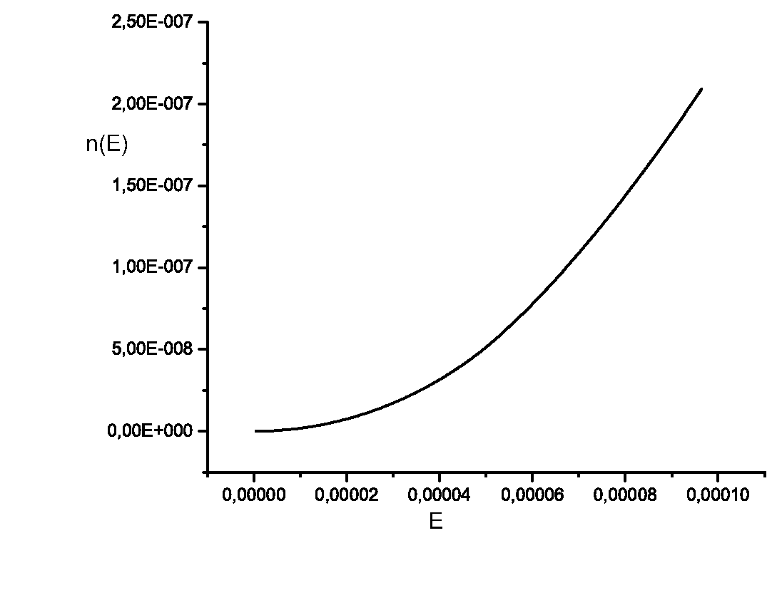
Figure 6.1: Density $\rho(E)$ (left) and staircase number $n(E)$ (right) for $\hbar=1$ in Thomas-Fermi approximation in the $QO$ potential (2.3).

As a result the original spectrum is transformed to quasi-equidistant:

$$\rho(\varepsilon)=1.$$

Only for spectra transformed that way does it make sense to discuss the quantum signatures of chaos in the statistical properties of energy spectra.

6.2 Nearest neighbor spacing distribution function

In the 1960s of last century Wigner [47], Porter [48] and Dyson [49] built statistical theory of complex systems spectra on the basis of the following hypothesis: energy levels distribution in complex systems is equivalent to distribution of the eigenvalues of random matrices ensemble with certain symmetry. The ultimate result for FNNS obtained in that theory has the following form:

$$P(S)\sim aS^{\alpha}e^{-bS^{2}},$$

where $a$ and $b$ are slowly varying functions of energy and critical exponent $\alpha$; defining behavior of the distribution function in the limit $S\rightarrow 0$, depends on symmetry properties of the random matrices: $\alpha=1$ for orthogonal and $\alpha=2$ for unitary ensemble of matrices.

Predictions of the statistical theory of energy spectra (mainly for Gaussian orthogonal ensemble of random matrices) were carefully compared with all available data on nuclear spectra. No considerable contradictions between the theory and experiment were found. In particular, the random matrices ensembles perfectly reproduced such an important spectral characteristic as spectral rigidity, describing small fluctuations of energy levels around averaged values in a given interval. Measure of rigidity is the statistic $\Delta_{3}$ of Dyson [49] and Mehta [50]

$$\Delta_{3}(L;x)=\frac{1}{L}\min\limits_{A,B}{\int\limits_{x}^{x+L}[n(\varepsilon)-A\varepsilon-B]^{2}d\varepsilon}$$ (6.7)

which determines the least-square deviation of the staircase representing the cumulative density $n(\varepsilon)$ from the best straight line fitting it in any interval $[x,x+L]$. The most perfectly rigid spectrum is the picket fence with all spacing equal (for instance, the one-dimensional harmonic oscillator spectrum), therefore maximally correlated, for which $\Delta_{3}=1/12$, whereas, at the opposite extreme the Poisson spectrum has a very large average value of rigidity $(\Delta_{3}=L/15)$, reflecting strong fluctuations around the mean level density.

Analogous comparisons were made also for atomic spectra. Good agreement with theory was found for them too, although for much poorer statistics.

A completely different approach to the problem of statistical properties of energy spectra was developed on the basis of non-linear theory of dynamical systems. As numerical simulations show [51, 52, 53, 54], confirmed by serious theoretical considerations [2, 3, 52, 56], the main universal property of systems which have regular type of dynamics in the classical limit, is the level clustering phenomenon, while for systems that are chaotic in the classical limit level repulsion is observed. This statement sometimes is called the hypothesis of universal character of energy spectra fluctuations [51].

In the case of regular motion any classical trajectory lies on a surface topologically equivalent to a torus. Each such torus corresponds to a certain set of integrals of motions (or quantum numbers), with the total number equal to the number of degrees of freedom. Different eigenfunctions of integrable quantum systems correspond to different sets of quantum numbers, and therefore lie on different tori. Their eigenenergies are not correlated, which leads to Poissonian FNNS

$$P_{P}(S)=e^{-S}$$ (6.8)

responsible for level clustering.

In the transition to chaos some tori are destroyed, leading to formation of chaotic regions in the phase space. Classical trajectories in such regions diffuse between different (already destroyed) tori. Therefore different chaotic modes can be represented in the form of superposition of former regular modes, which leads to repulsion between the corresponding levels. In the limit of a completely chaotic system, all modes of initially integrable system mix one with other, so that repulsion exists between any pair of levels, changing FNNS from Poissonian to the Wigner one:

$$P_{W}(S)=\frac{\pi}{2}Se^{-\frac{\pi}{4}S^{2}}.$$ (6.9)

The situation became more complicated for generic Hamiltonian systems, where the phase space contains both regular and chaotic components. How is it reflected in the energy spectra statistical properties?

Historically the first was the phenomenological approach to the solution of that problem, proposed by Brody [57], who considered FNNS of the form:

$$P_{B}(S)=(\beta+1)bS^{\beta}e^{-bS^{\beta+1}},\ b=\left[\Gamma\left(1+\frac{1}{\beta+1}\right)\right]^{\beta+1}$$ (6.10)

where $\beta$ equals to the relative measure of classical phase space, occupied by the chaotic trajectories: $\beta=0$ for regular and $\beta=1$ for chaotic systems.

Berry and Robnik [58] and independently Bogomolny [59] using on semiclassical arguments, showed that FNNS in the case of mixed type dynamics represents the superposition of Poisson and Wigner distributions with weights that are determined by the relative phase space measure of regular and chaotic motion respectively:

$$\begin{array}[]{c}P_{BRB}=\frac{d^{2}}{dS^{2}}\left[e^{-\rho S}erfc\left(\frac{\sqrt{\pi}}{2}(1-\rho)S\right)\right]=\\ =\rho^{2}e^{-\rho S}erfc\left(\frac{\sqrt{\pi}}{2}(1-\rho)S\right)+(1-\rho)\left(2\rho+\frac{\pi}{2}(1-\rho)^{2}S\right)e^{-\rho S-\frac{\pi}{4}(1-\rho)^{2}S^{2}}\end{array}$$ (6.11)

where $\rho$ is the relative phase volume occupied by regular trajectories in the mixed system. The limit $\rho\rightarrow 1$ corresponds to regular system, and $\rho\rightarrow 0$ — to completely chaotic.

Further development theory of FNNS acquired in the works of Narimanov and Podolskiy [60], who accounted for additional effect of repulsion for close levels due to dynamical tunneling (more details see Chapter 8):

$$\begin{array}[]{c}P_{NP}=\rho^{2}F\left(\frac{S}{\nu^{2}}\right)e^{-\rho S}erfc\left(\frac{\sqrt{\pi}}{2}(1-\rho)S\right)+\\ +(1-\rho)\left(2\rho F\left(\frac{S}{\nu^{2}}\right)+\frac{\pi}{2}(1-\rho)^{2}S\right)e^{-\rho S-\frac{\pi}{4}(1-\rho)^{2}S^{2}}\\ F(x)=1-\frac{1\sqrt{\frac{\pi}{2}}x}{e^{x}-x}.\end{array}$$ (6.12)

The $\rho$ parameter in the Narimanov-Podolskiy distribution function (6.12) has the same physical sense as in the Berry-Robnik-Bogomolny distribution (6.11), and additional parameter $\nu$ is connected to the intensity of dynamical tunneling. Therefore the Berry-Robnik-Bogomolny distribution function represents a particular case of the Narimanov-Podolskiy distribution at $\nu=9$, which corresponds to the absence of the tunneling (Fig.6.2).

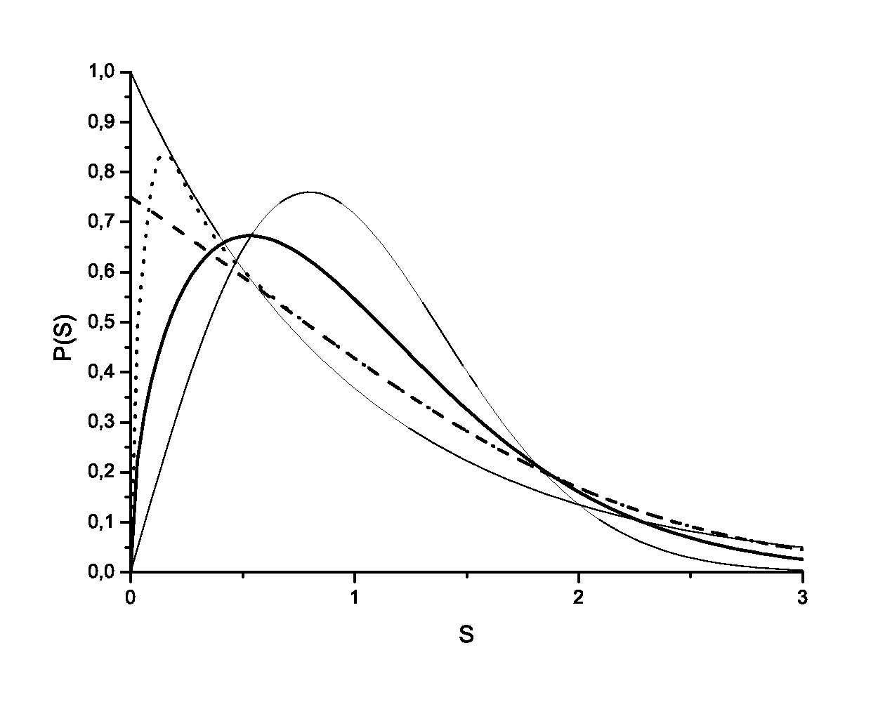
Figure 6.2: The distribution functions of Poisson and Wigner (thin solid lines), Brody for $\beta=0.5$ (thick solid line), Berry-Robnik-Bogomolny for $\rho=0.5$ (dashed line) and Narimanov-Podolskiy for $\rho=0.5$ and $\nu=0.1$ (dotted line)

Among systems subject to extensive numerical analysis of the spectral properties, two-dimensional billiards possess the central place. The two-dimensional billiard represents a point particle freely moving on the plane inside some region of arbitrary shape and elastically reflecting from the boundary. Such systems attract active interest in research for the following reasons:

1. the system has the lowest possible number of degrees of freedom, allowing chaotic motion in a conservative system;

2. the simplicity of classical dynamics;

3. stochasticity criteria for billiards are formulated in geometrical terms;

4. homogeneity of the phase space;

5. availability of efficient methods for solution of the Schrödinger equation for billiards;

6. smooth component of level density is well known due to the Weyl formula;

7. billiard dynamics reflect the real situation in many physical systems (quantum dots and antidots, Josephson’s junctions, nuclear billiards)

8. at the present time there is efficient experimental realization both for classical and quantum dynamics in microwave and optical two-dimensional resonators.

For billiards with certain boundary shape one of two limiting cases is realized: exact integrability or absolute chaos. So in the circular billiard (Fig.6.3a) angular momentum is the second (after energy) integral of motion, and this system is integrable. A billiard of ”stadium” type (Fig.6.3b) is one of the simplest stochastic systems. In Fig.6.3 the statistical characteristics of energy spectra (FNNS and dispersion) are presented for both systems. In complete agreement with the hypothesis of the universal character of spectral fluctuations, FNNS for the circular billiard is perfectly approximated by Poissonian distribution, and dispersion is a linear function of the length of the considered interval. In the non-integrable case the level repulsion effect is pronouncedly manifested, leading to Wigner distribution, and dispersion grows much more slowly because of the higher rigidity of the considered spectrum.

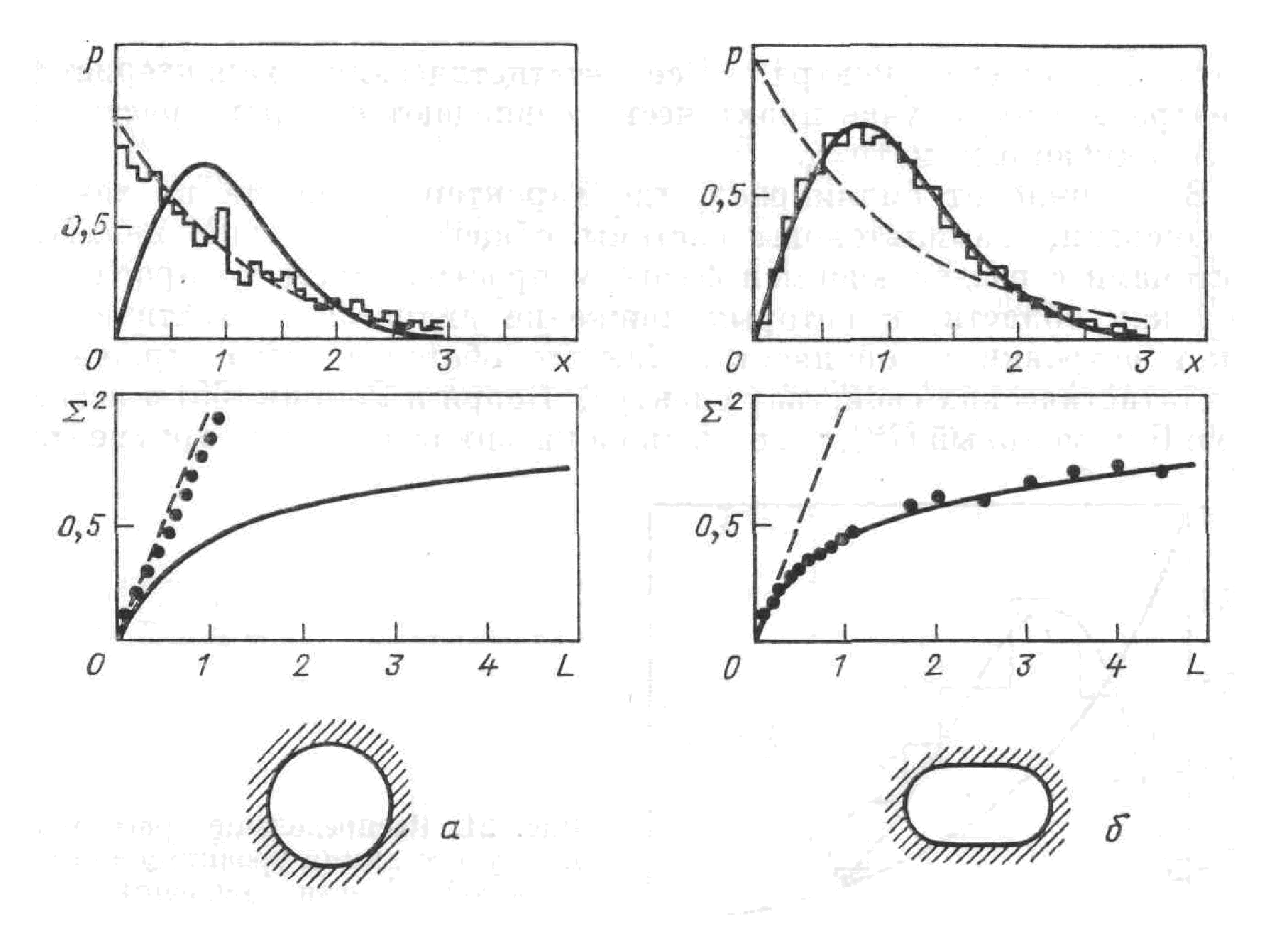
Figure 6.3: Statistical characteristics of energy spectra for circular (a) and ”stadium” (b) billiards.

6.2.1 Uniform potential case

Let us note that an important advantage of billiards is the possibility of spectrum unfolding (6.6) with high precision and independence of relative measures of regular and chaotic components from the energy of particles. Both features equally share homogeneous potentials, in particular coupled quartic oscillators potential (5.22), where we consider for simplicity only $A_{1}$-type states — even on both coordinates and symmetric with respect to exchange $x\leftrightarrow y$.

As for quantum billiards, for the coupled quartic oscillators potential (5.22) there is a quite precise semiclassical expression for the smooth component of staircase state number function up to the third order in energy [96]:

$$\bar{n}_{A_{1}}(E)\simeq\frac{E^{\frac{3}{2}}}{48}\left[F\left(\frac{1}{2},\frac{1}{2},1,\frac{2-\alpha}{4}\right)+6\frac{\frac{\Gamma\left(\frac{5}{4}\right)}{2^{\frac{5}{4}}}+\frac{1}{\alpha+2}}{\Gamma\left(\frac{7}{4}\right)\sqrt{2\pi E^{\frac{3}{2}}}}+\frac{9}{2E^{\frac{3}{2}}}\right],$$ (6.13)

which allows us to perform spectrum unfolding with sufficiently high accuracy in a wide energy range. However because of technical difficulties in numerical calculation of hypergeometric function in (6.13), in practice it is much more convenient to use the corresponding Thomas-Fermi approximation for (6.13) in the form:

$$\bar{n}_{A_{1}}(E)\approx\frac{E^{\frac{3}{2}}}{12}\int\limits_{0}^{\frac{\pi}{2}}\frac{d\varphi}{\sqrt{1+\frac{\alpha-2}{4}\sin^{2}\varphi}}.$$ (6.14)

It is convenient to estimate the accuracy of the spectrum unfolding with a diagram of variable $\varepsilon_{n}/n$ plotted for all levels in the spectral series under consideration. For a spectrum standardly unfolded by (6.6), this variable should be sufficiently close to unity in the whole energy interval. As can be seen from Fig.6.4, the Thomas-Fermi approximation(6.14) gives slightly understated values for $\bar{n}_{A_{1}}(E)$, but nevertheless allows us to achieve $1\%$ accuracy of spectrum unfolding, and this accuracy improves with energy growth.

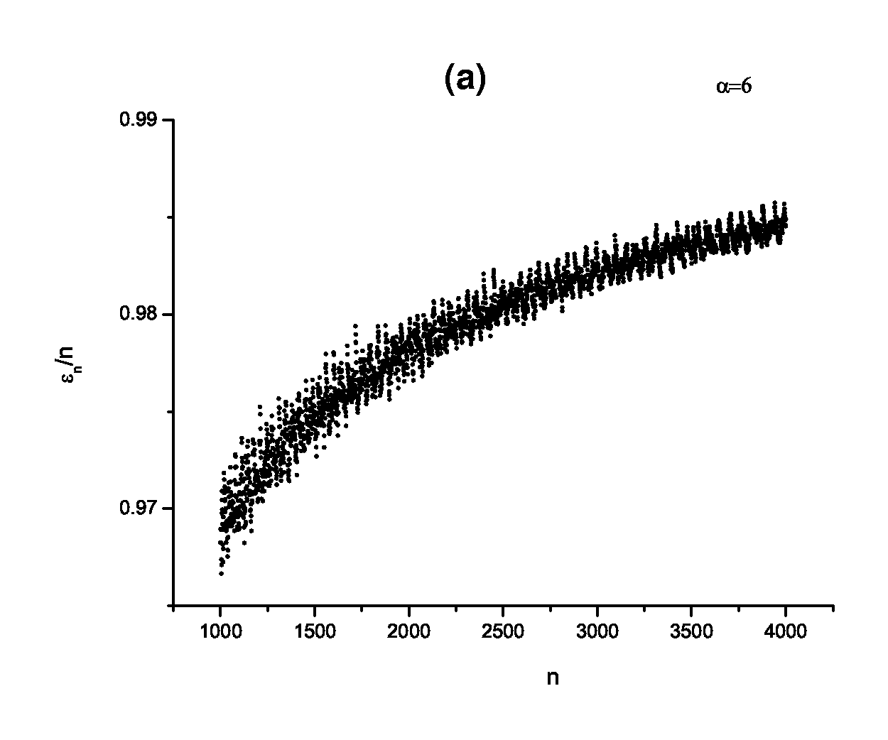
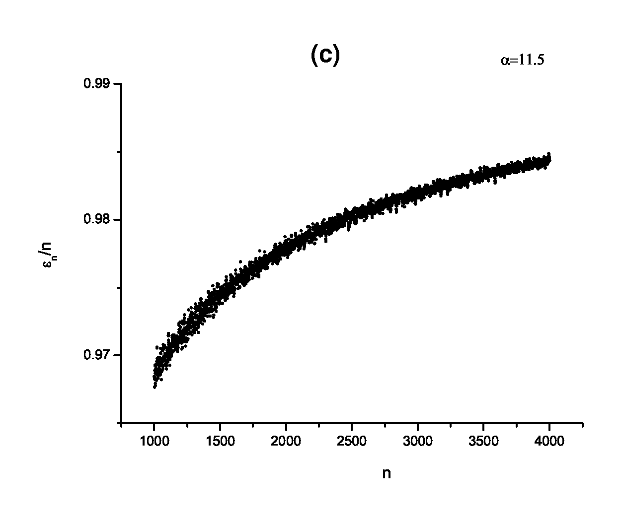
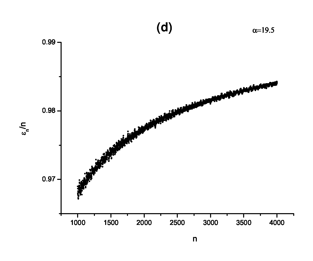
Figure 6.4: Accuracy estimation for the unfolding with (6.13) in the spectrum of coupled quartic oscillator potential (5.22) for $\alpha=6$(a), $\alpha=7.5$(b), $\alpha=11.5$(c), $\alpha=19.5$(d).

In Fig.6.4 one can see gradual decrease of maximum amplitude of the spectral fluctuations with growth of chaoticity measure (see Fig.6.5), which already qualitatively points to gradual changes of the fluctuations character from Poissonian (Fig.6.4a) to Wigner one (Fig.6.4d).

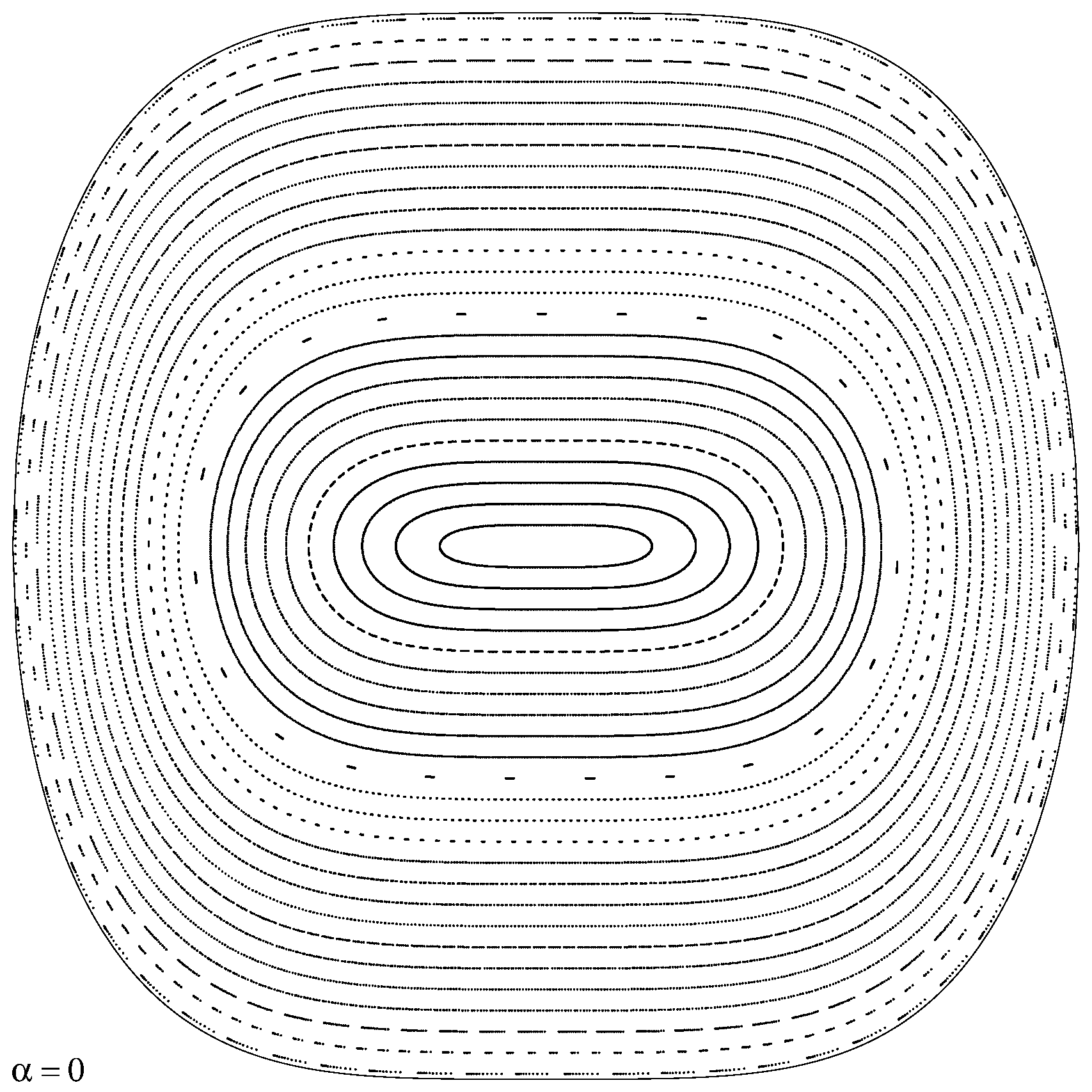
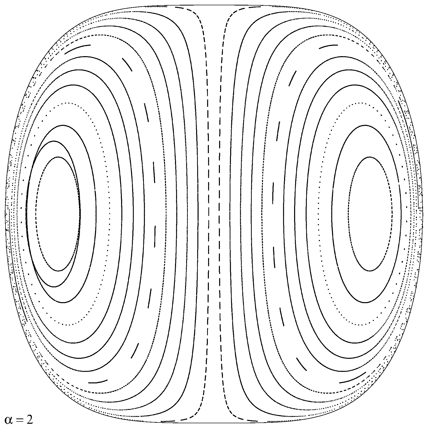
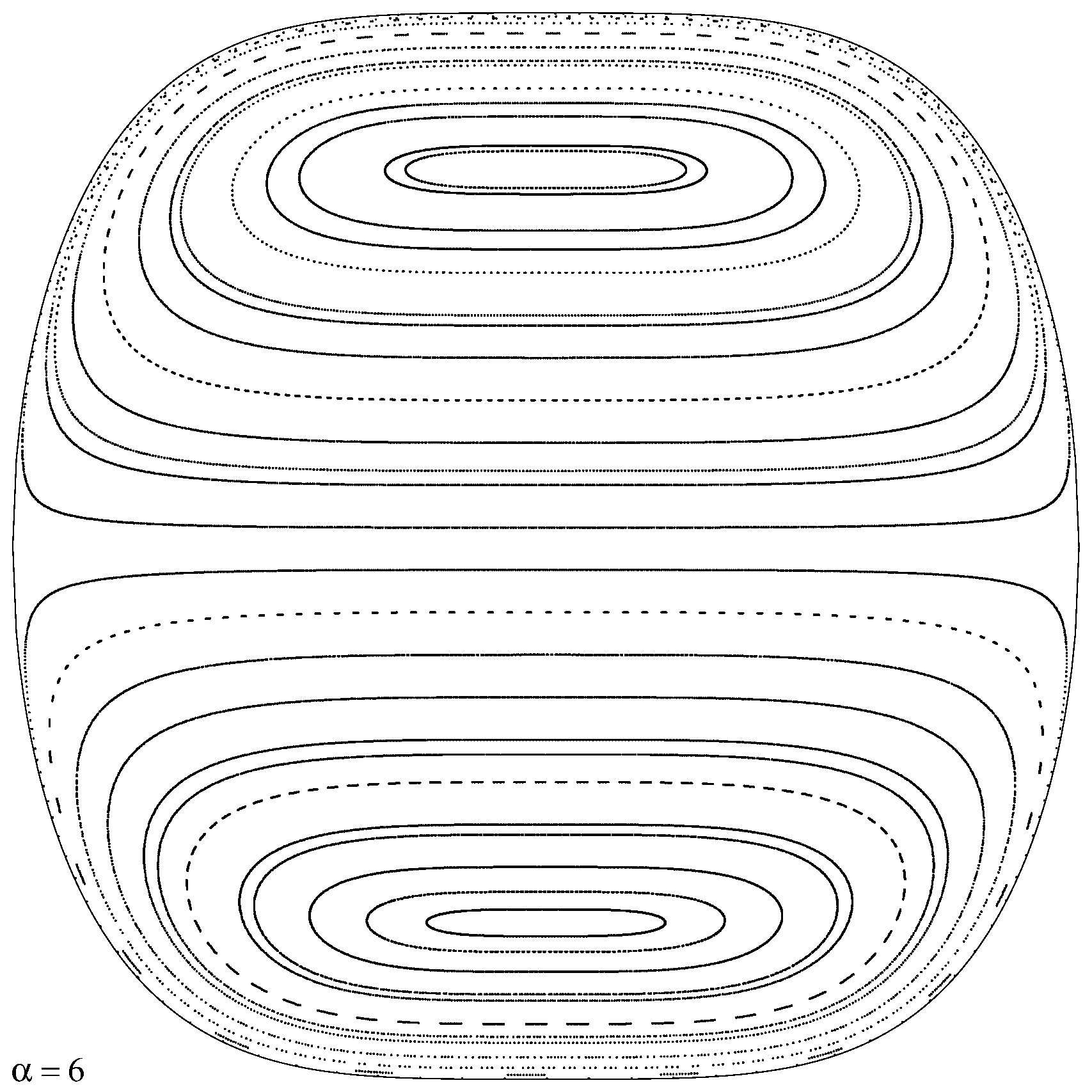
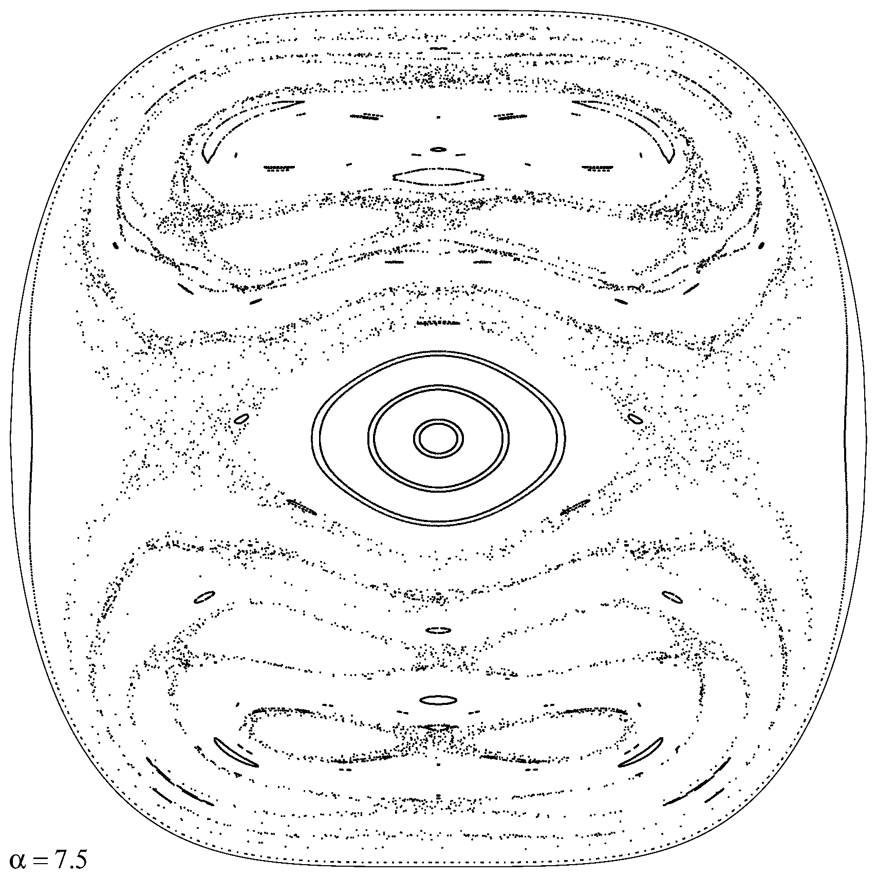
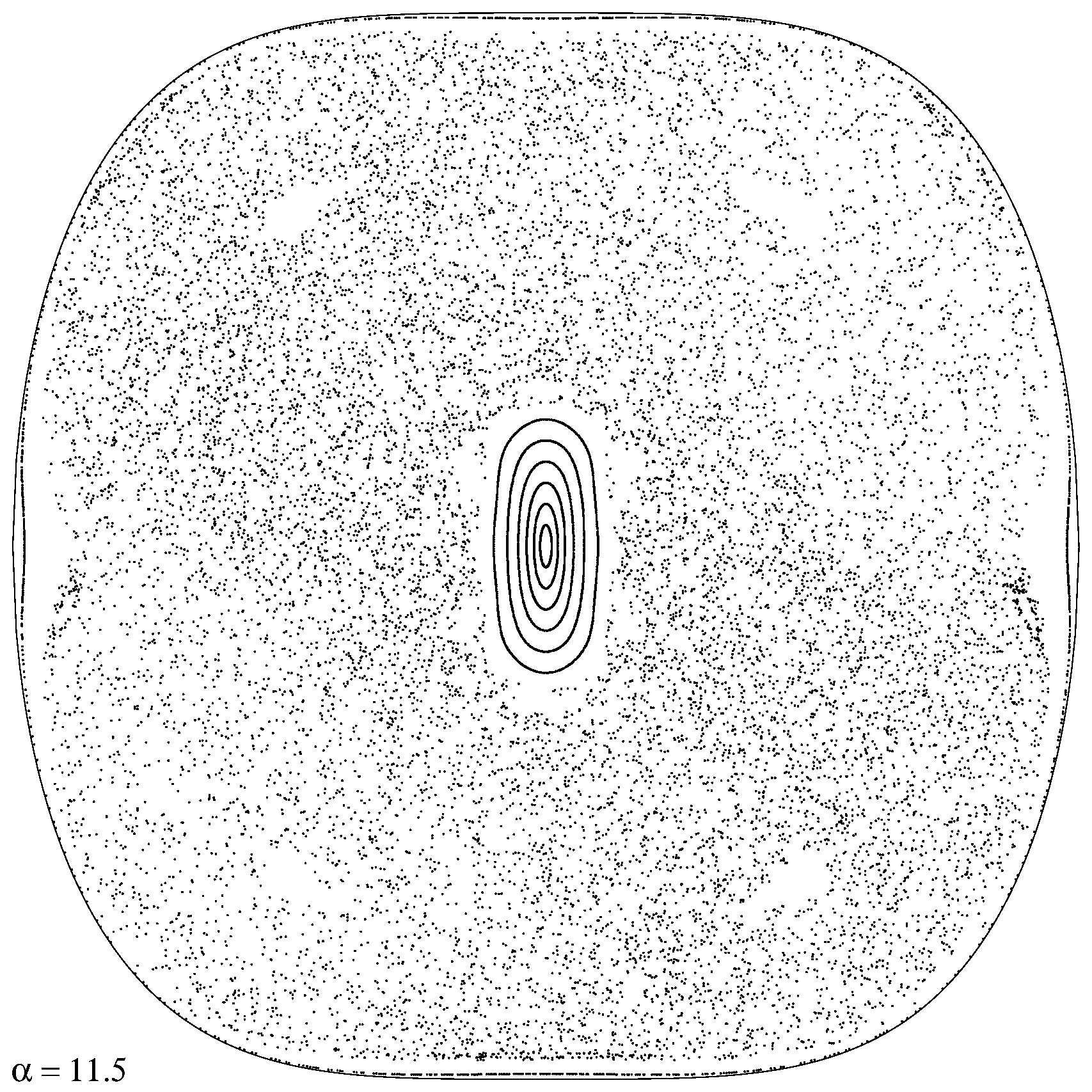
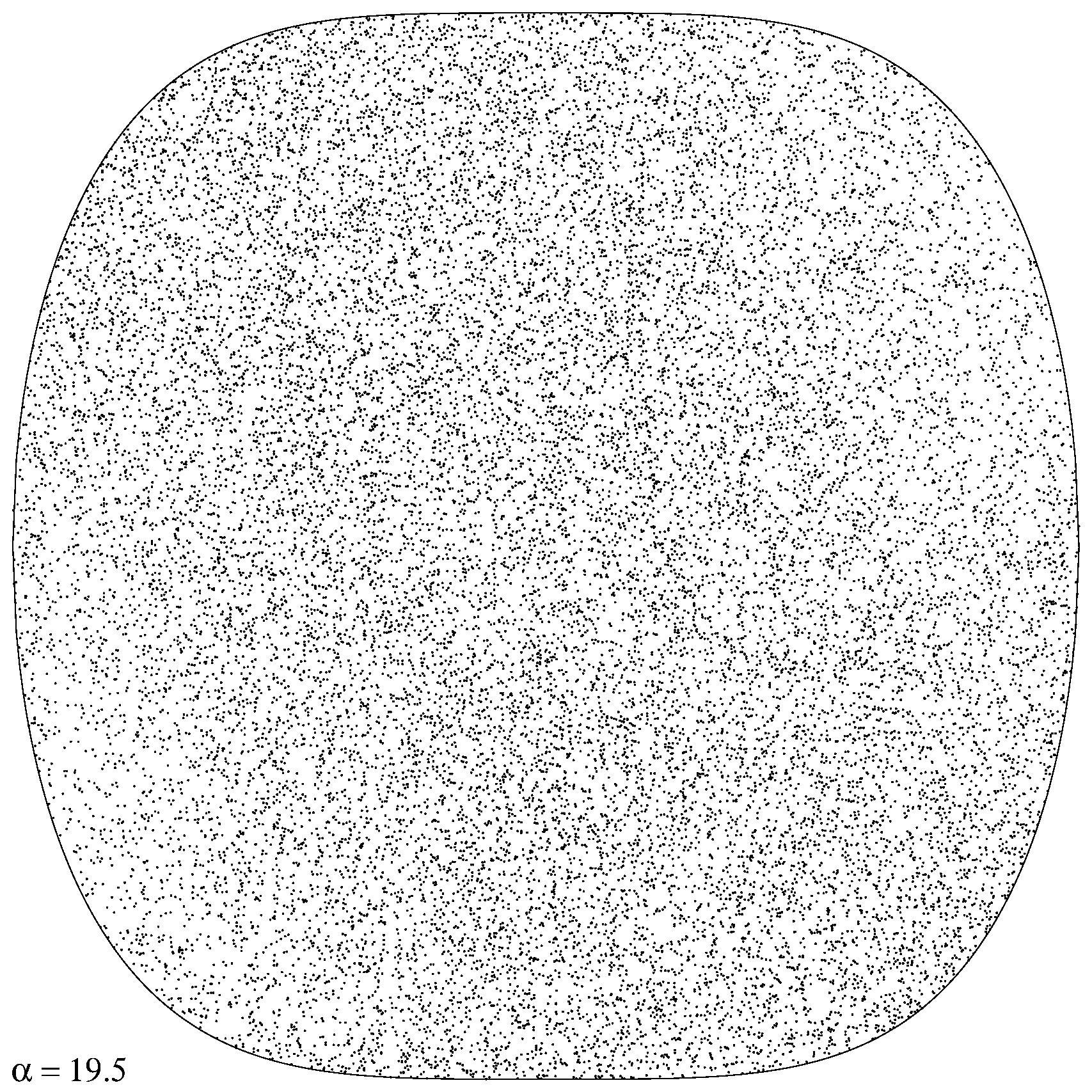
Figure 6.5: Poincaré surfaces of section in the $(x,p_{x})$ plane for the coupled quartic oscillator potential with coupling constant $\alpha=0,2,6,7.5,11.5,19.5$. The solid line limits the classically allowed region of the phase space.

The FNNS for coupled quartic potential (5.22) together with the best fits by Brody (6.10) and Berry-Robnik-Bogomolny (6.11) distributions are presented in Fig.6.6 in normal and on Fig.6.7 in logarithmic scale. The latter is especially convenient because in the logarithmic representation the Poissonian distribution turns into linear function:

$$\ln P_{P}(S)=-S,$$

and proximity of numerically obtained distribution to Poissonian one in the case of regular motion (Fig.6.7) becomes especially clear.

According to the hypothesis of univeral character of spectral fluctuations the FNNS transforms from Poissonian at $\alpha=6$ to Wigner one at $\alpha=19.5$. In the intermediate cases the numerical distribution function is satisfactorily described by the Berry-Robnik-Bogomolny distribution as well as Brody distribution, and the latter gives even better accuracy regardless of its phenomenological nature.

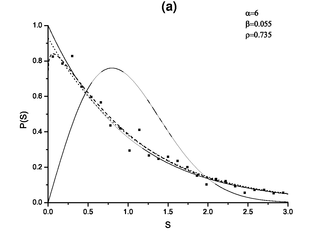
Figure 6.6: FNNS for the coupled quartic oscillator potential (5.22) for $\alpha=6$(a), $\alpha=7.5$(b), $\alpha=11.5$(c), $\alpha=19.5$(d). Points represent numerical data, solid lines — Poisson (6.8) and Wigner (6.9) distributions, dashed and dotted lines — the best fits by the Brody (6.10) and the Berry-Robnik-Bogomolny (6.11) distributions respectively.

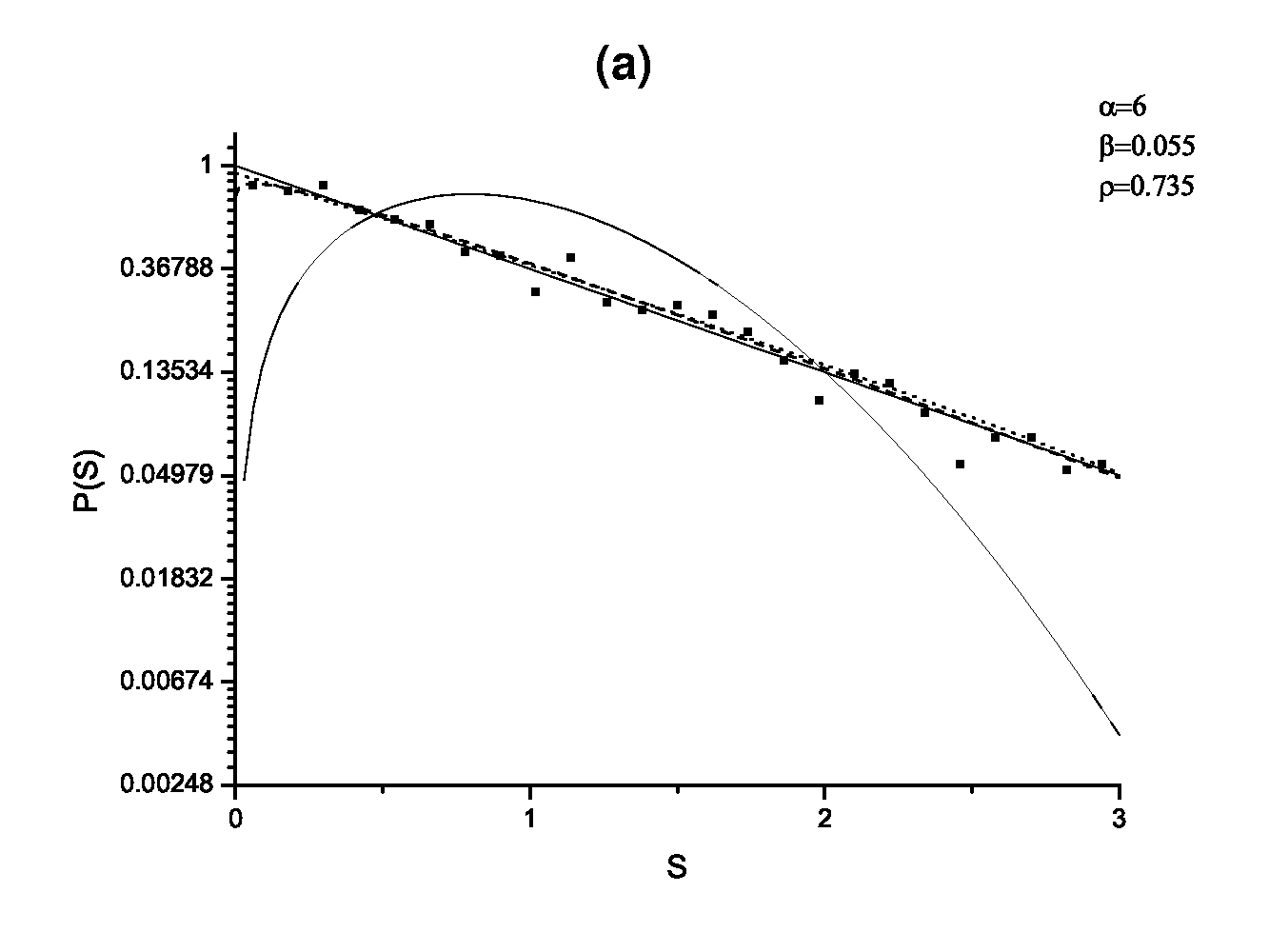
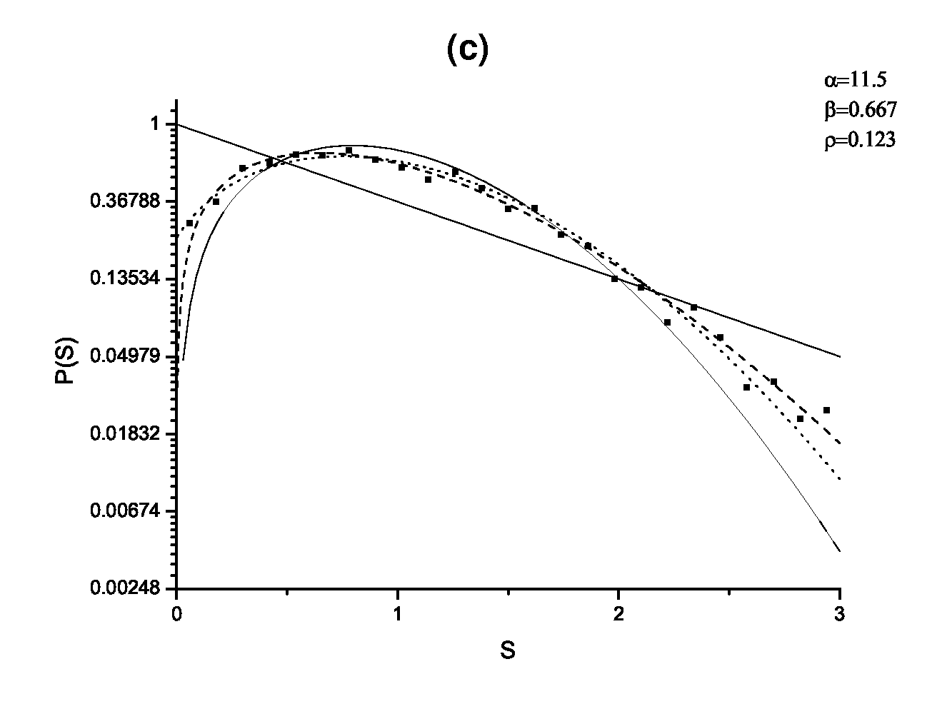
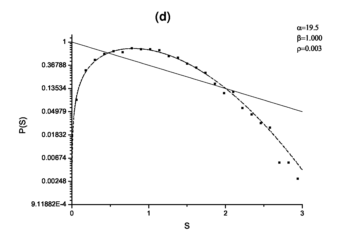
Figure 6.7: The same as on Fig.6.6 but in logarithmic scale.

Distributions on Fig.6.6 and Fig.6.7 are obtained from analysis of spectral series consisted of $3000$ levels each, but even these statistics appears too low to give preference to Brody distribution over the Berry-Robnik-Bogomolny distribution. In the case of too pure statistics which is common in smooth potentials it is better to use integral, or cumulative distribution:

$$W(S)=\int\limits_{0}^{S}P(S)dS$$

It is easy to obtain cumulative distributions corresponding to Brody and Berry-Robnik-Bogomolny distributions:

$$\begin{array}[]{c}W_{B}(S)=1-e^{-bS^{\beta+1}}\\ W_{BRB}(S)=1+\frac{d}{dS}\left[e^{-\rho S}erfc\left(\frac{\sqrt{\pi}}{2}(1-\rho)S\right)\right]\end{array}$$ (6.15)

Cumulative Poisson and Wigner distributions, as well as the usual ones, are limiting cases of the Brody distribution at $\beta=0$ and $\beta=1$ and of the Berry-Robnik-Bogomolny one at $\rho=1$ and $\rho=0$ respectively:

$$\begin{array}[]{c}W_{B}(S)=1-e^{-S}\\ W_{BRB}(S)=1-e^{-\frac{\pi}{4}S^{2}}\end{array}$$ (6.16)

The numerically obtained cumulative FNNS for coupled quartic potential (5.22) together with the best fits by the Brody and Berry-Robnik-Bogomolny (6.15) distributions are presented in Fig.6.8. It should be noted that parameters of the best fit made independently by usual (6.10,6.11) and cumulative (6.15) distributions agree one with another very well. However cumulative distributions demonstrate better agreement with numerical data exactly for the Brody distribution rather than for the Berry-Robnik-Bogomolny distribution. The usual explanation of that fact states that the Berry-Robnik-Bogomolny distribution is a theoretically well-grounded universal high-energy asymptote for FNNS but it has limited applicability for insufficiently high energies. Therefore level fluctuations in the spectral series available for most potential systems are better described by phenomenological Brody distribution (6.10).

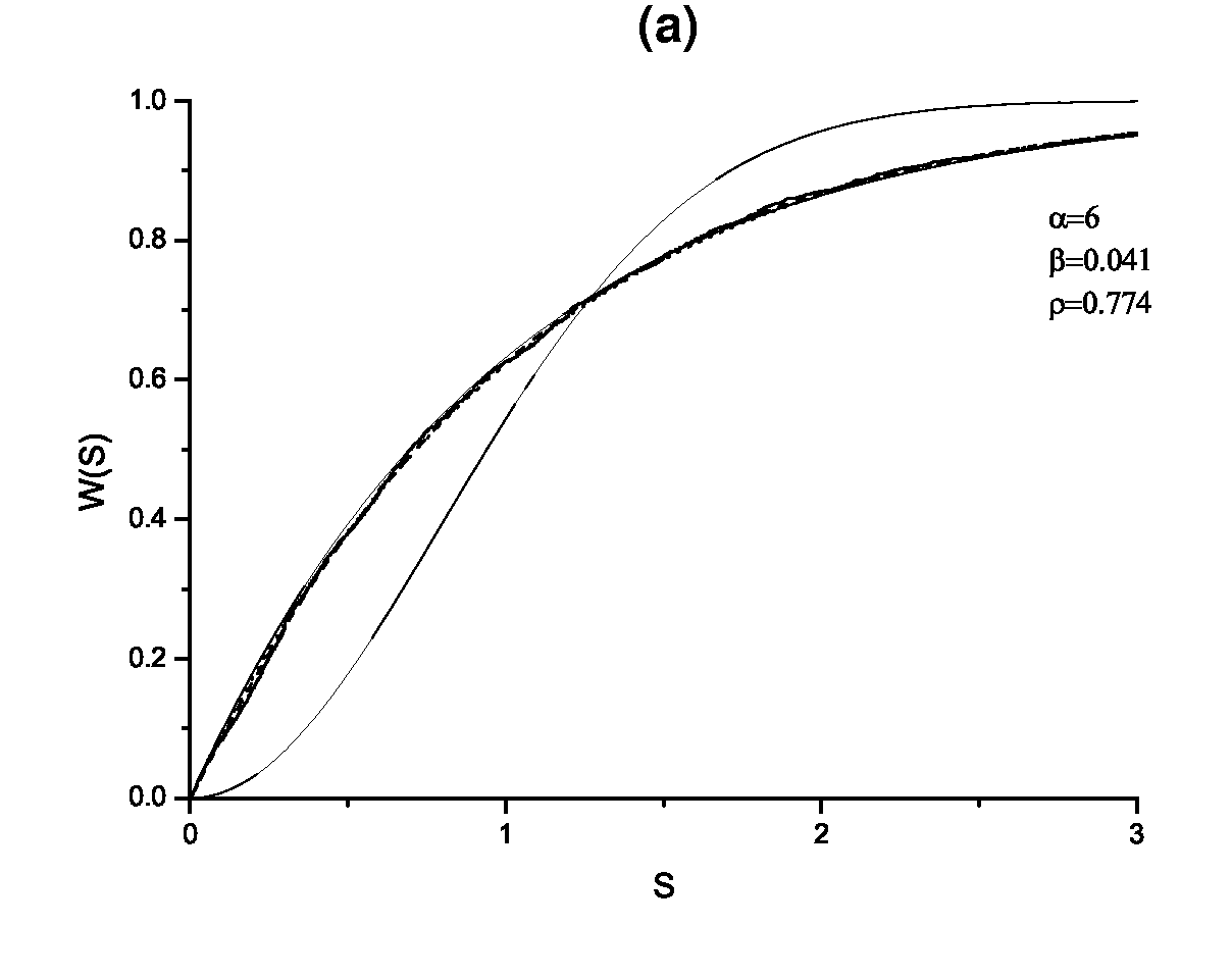
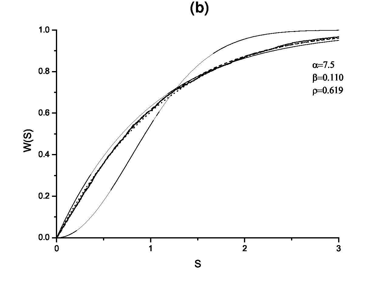
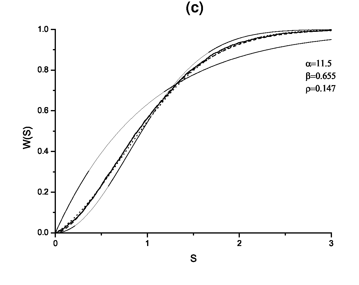
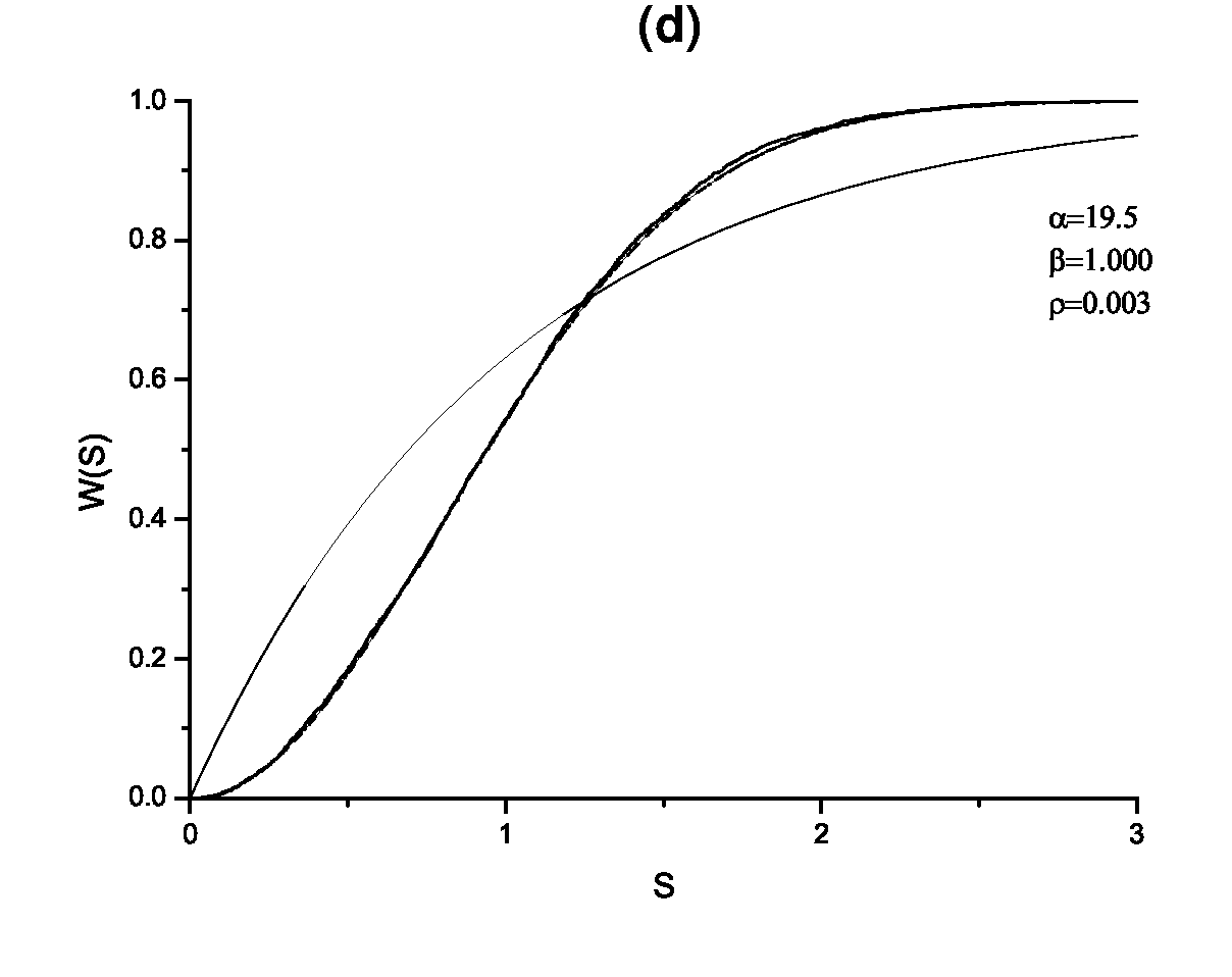
Figure 6.8: The cumulative FNNS for the coupled quartic oscillator potential (5.22) for $\alpha=6$(a), $\alpha=7.5$(b), $\alpha=11.5$(c), $\alpha=19.5$(d). Points represent numerical data, solid lines — Poisson and Wigner (6.16) distributions, dashed and dotted lines — the best fits by the Brody and the Berry-Robnik-Bogomolny (6.15) distributions respectively.

The most striking distinction between the Brody and Berry-Robnik-Bogomolny distributions is displayed in the so-called $T$-representation:

$$T(S)=\ln\{-\ln[1-W(S)]\}.$$

In the variables $(T,\ln T)$ the Brody distribution with any parameter $\beta$, as well as Poisson and Wigner distributions, become linear functions:

$$T_{B}(S)=\ln b+(\beta+1)\ln S\\$$ (6.17)

$$\begin{array}[]{l}T_{P}(S)=\ln S\\ T_{W}(S)=\ln\frac{\pi}{4}+2\ln S,\end{array}$$ (6.18)

which is not the case for the Berry-Robnik-Bogomolny distribution:

$$T_{BRB}=\ln\left\{-\ln\left(\frac{d}{dS}\left[e^{-\rho S}erfc\left(\frac{\sqrt{\pi}}{2}(1-\rho)S\right)\right]\right)\right\}.$$ (6.19)

The slope of the $T$-distribution on the $(T,\ln T)$ determines the repulsion rate in the model (6.7): Wigner distribution corresponds to linear repulsion and Poisson distribution — to zero, or absence of repulsion. Therefore to the Brody distribution we can assign so-called fractional levels repulsion with the exponent continuously changing from $0$ to $1$. At the same time the Berry-Robnik-Bogomolny distribution describes only integer repulsion with the exponent equal to $1$. As can be seen from Fig.6.9, the fractional level repulsion effect actually takes place in smooth potential systems and is correctly described by the Brody distribution.

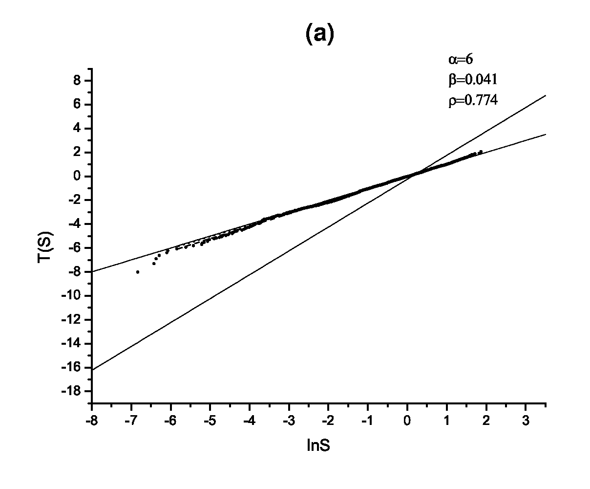
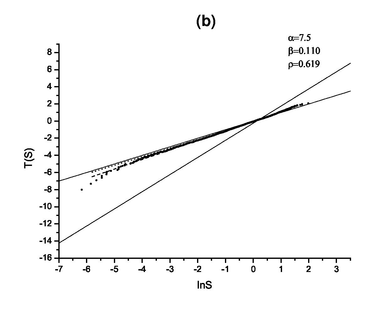
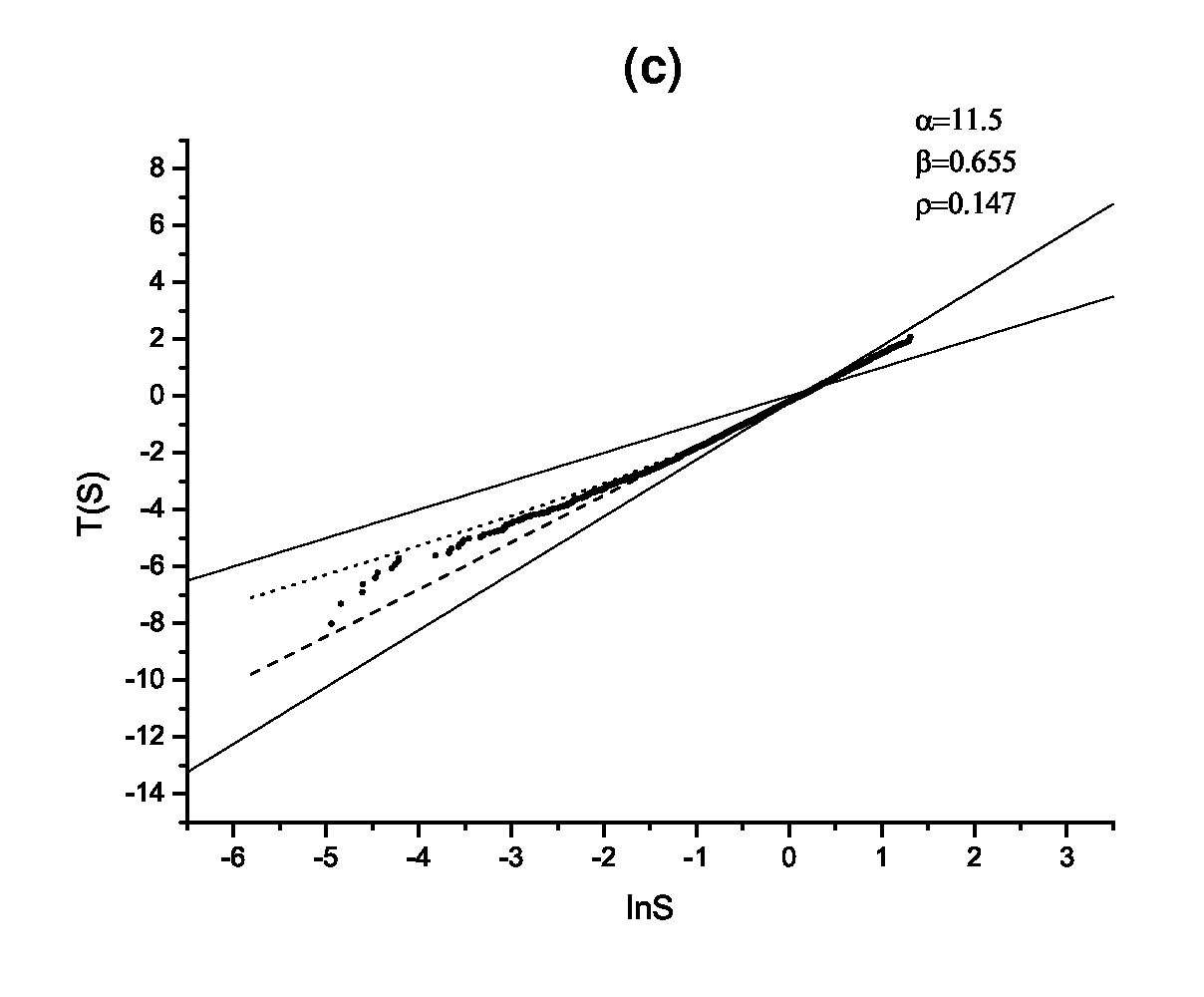
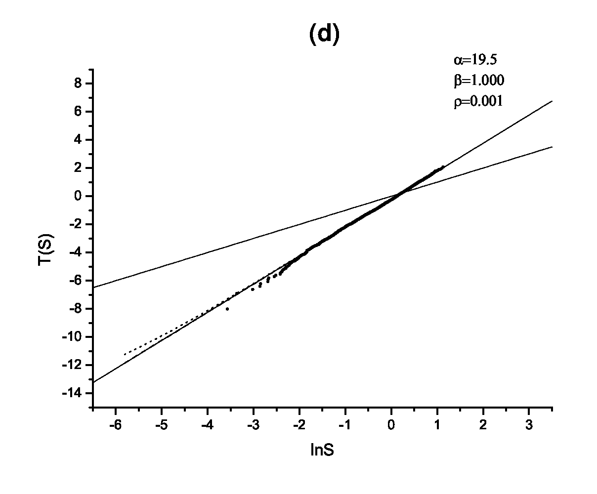
Figure 6.9: The cumulative FNNS in the $T$-representation for the coupled quartic oscillator potential (5.22) for $\alpha=6$(a), $\alpha=7.5$(b), $\alpha=11.5$(c), $\alpha=19.5$(d). Points represent numerical data, solid lines — Poisson and Wigner (6.18) distributions, dashed and dotted lines — the best fits by the Brody (6.17) and the Berry-Robnik-Bogomolny (6.19) distributions respectively.

6.2.2 Generic potential case

Let us pass now from the special case of uniform potentials to the more generic situation. Let us note at the beginning that, even in the case of non-uniform potentials in the presence of $R-C$ or $R-C-R$ transitions, it is possible to build rather representative series of energy levels corresponding to a definite type of classical motion. As an example let us consider the transformation of statistical properties of the energy spectrum of the quadrupole oscillations Hamiltonian (2.2) in the $R-C-R$ transition for one-well case $(W<16)$. At the fixed topology of potential surface $(W=const)$ the unique free parameter of the Hamiltonian is the scaled Planck’s constant $\bar{\hbar}$. In the study of the concrete energetic interval ($R_{1}$, $C$ or $R_{2}$), corresponding to a definite type of classical motion, the choice of $\bar{\hbar}$ is dictated by the possibility of attainment of the necessary statistical assurance (the required number of levels in the investigated energy interval) with conservation of precision of spectrum calculation (restrictions to possibility of diagonalization of matrices of large dimension). The numerical results are presented in Fig.6.10. Both the FNNS $p(x)$ and the average value of $\Delta_{3}$ well correspond to the predictions of GOE for the chaotic $(C)$ region. The logarithmic scale for $p(x)$ is suitable to trace this correspondence at large $x$. For regular regions ($R_{1}$ and $R_{2}$) the distribution function, in the same scale, according to the hypothesis of the universal character of fluctuations of energy spectra, must be represented by a straight line (the logarithm of Poisson’s distribution). The results demonstrate the agreement with this hypothesis, though small-sized deviations are observed for small distances between levels. Such a tendency to the rise of some repulsion in the regular region, apparently, is connected with a small admixture of chaotic components. At the construction of statistical characteristics, a purity of sequence is provided by using only those levels, which are relative to definite irreducible representation of $C_{3v}$ group (the levels of $E$-type were used for results represented in Fig.6.10; the statistical characteristics of levels of $A_{1}$ and $A_{2}$-types have similar form).

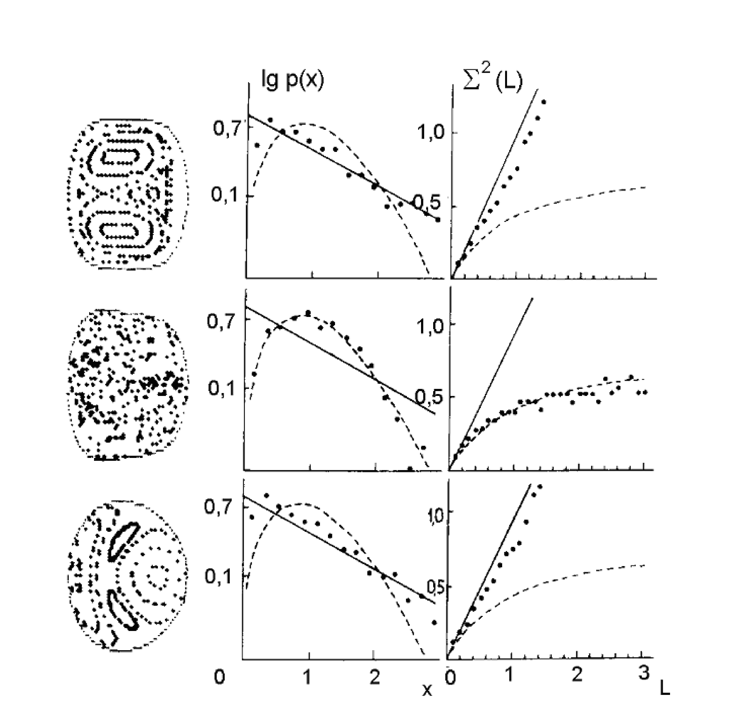
Figure 6.10: Correlation between the character of classical motion and statistical properties of energy spectra in $R-C-R$ transition for the Hamiltonian of quadrupole oscillations (2.2). On the left — Poincaré sections, in the middle — FNNS distribution $p(x)$, on the right — the variance $\Sigma^{2}$. From the bottom up: the first regular range $R_{1}$, the chaotic range $C$, the second regular range $R_{2}$

Spectral ranges of multi-well potentials realizing the mixed state open new possibilities for investigation of the intermediate statistics. At those energies chaotic and regular components are separated not only in Phase space as in the usual case of mixed type motion), but already in the configuration space. A priori the FNNS form in the mixed state is not necessarily reduced to definitely weighted superposition of Poisson and Wigner distribution. In that case we deal not with statistics of admixture of two level series with different FNNS, but with statistics of spectrum series, where each level cannot be attributed to definite (Poisson or Wigner) statistics. Statistical properties of such systems have not been under study up to now although they are the systems corresponding to the common case situation.

Let us consider the simplest potential realizing the mixed state — two-well potential of lower umbilic catastrophe $D_{5}$ (2.4). In order to describe the statistical properties of the corresponding energy spectrum, let us try to use the Berry-Robnik-Bogomolny distribution (6.11), where the $\rho$ parameter equals the relative phase volume occupied by regular trajectories. In the case of $D_{5}$ potential $\rho\sim 1$ for $E<E_{cr}$ and $\rho\sim 1/3$ for $E>E_{cr}$, which qualitatively agree with numerical data for energy levels statistics Fig.6.11

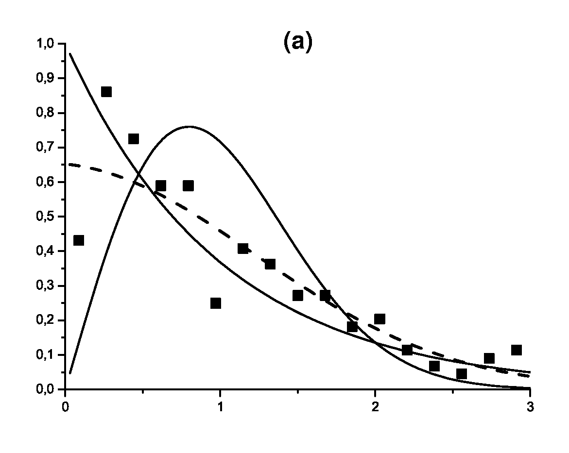
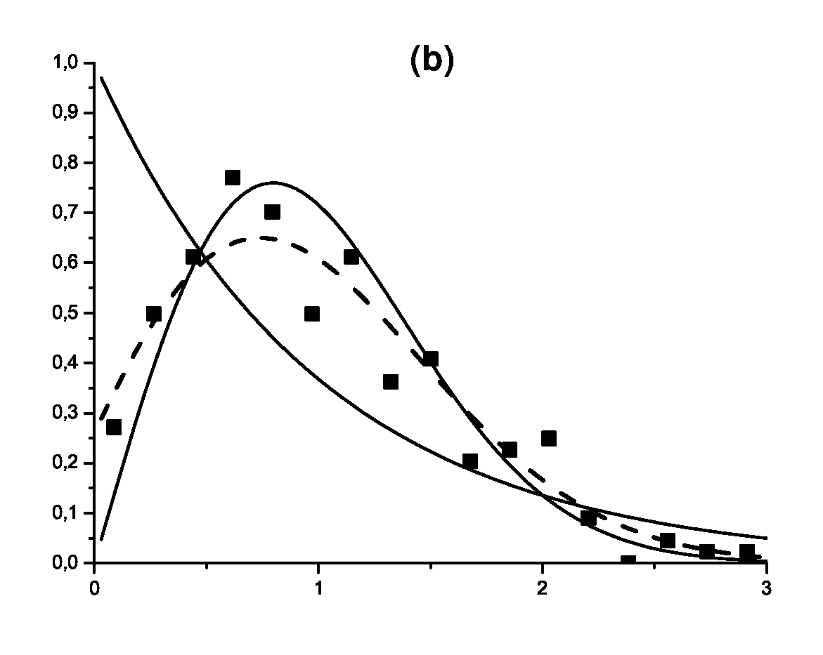
Figure 6.11: FNNS for the $D_{5}$ potential (2.4) for $E<E_{cr}$(a) and $E>E_{cr}$(b). Points represent numerical data, solid lines — Poisson (6.8) and Wigner (6.9) distributions, dashed line — the best fit by the Berry-Robnik-Bogomolny (6.11) distribution.

The Berry-Robnik-Bogomolny distribution function by its construction describes the energy level fluctuations in the absence of interaction between the regular and chaotic components. Therefore the best agreement between the Berry-Robnik-Bogomolny spectral fluctuations theory and experimental data we should expect exactly in the mixed state spectra, where interaction of chaotic and regulat states each with other is additionally suppressed by the energy barrier separating the corresponding local minima. In practice however such agreement is never observed for several reasons.

The first reason is not connected immediately with the mixed state properties and lies in technical difficulties of calculation of long spectral series in potentials with several local minima. In practice one usually should be happy with a series of several hundred levels at most, which is definitely insufficient to obtain accurate distribution functions for spectral fluctuations. Another difficulty of a technical nature is connected with the fact that the multiplicity of generic smooth potentials does not allow any systematic semiclassical analysis, because in particular there are no sufficiently precise semiclassical approximations for the smoothed component of staircase states number function, required for the standard unfolding procedure (6.6). Therefore in order to unfold the spectra we should be happy with the zero semiclassical approximation, i.e. usual Thomas-Fermi approximation, which for even states in the $D_{5}$ potential takes the following form:

$$\begin{array}[]{c}\bar{n}(E)=\bar{n}_{R}(E)+\bar{n}_{C}(E)\\ \bar{n}_{R,C}(E)\approx\frac{1}{3\pi\hbar^{2}}\int\limits_{\sqrt{2(1-\sqrt{E})}}^{\sqrt{2(1+\sqrt{E})}}\frac{dx}{\sqrt{x\pm 2}}\left[E-\left(\frac{x^{2}}{2}-1\right)^{2}\right]^{\frac{3}{2}},\end{array}$$ (6.20)

where $\bar{n}_{R}(E)$ and $\bar{n}_{C}(E)$ represent partial contributions from regular and chaotic minima respectively. Such a simple approximation nevertheless allows us to perform the spectrum unfolding with maximum errors of order $1\%$ in the whole energy interval of interest (see Fig.6.12).

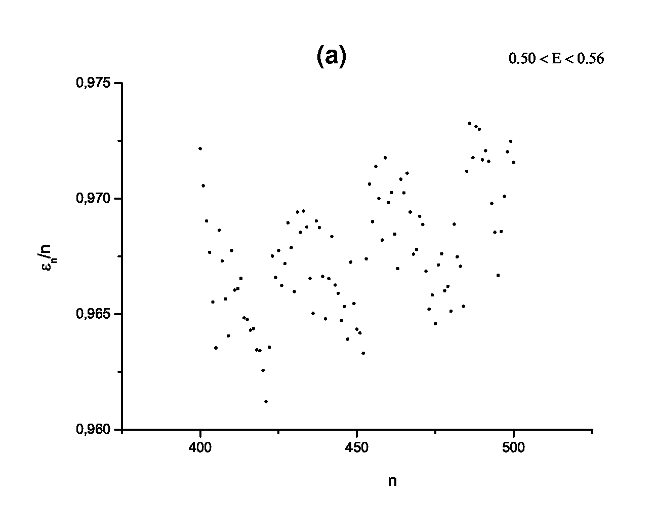
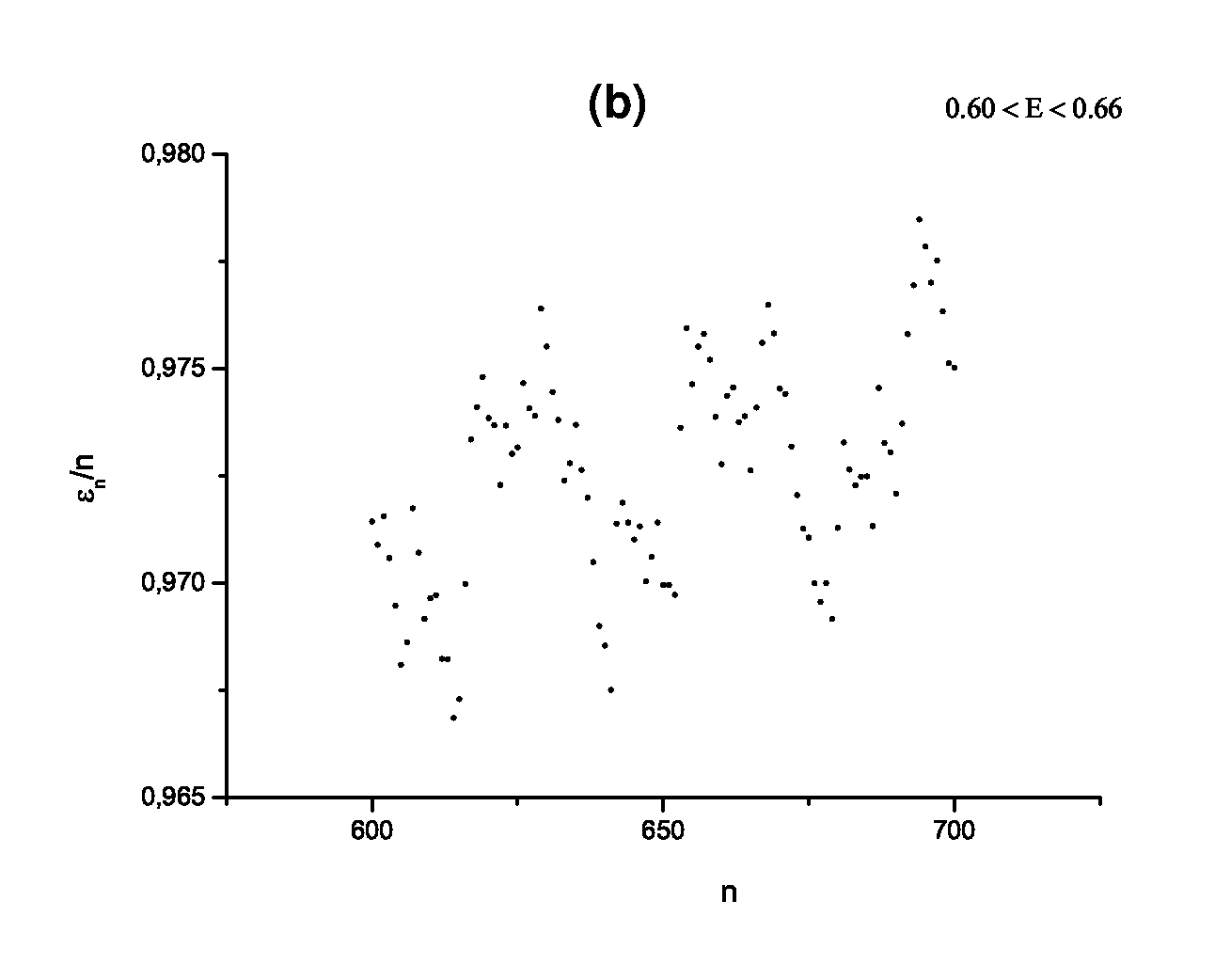
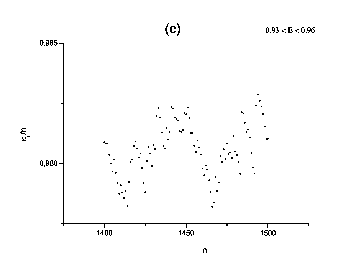
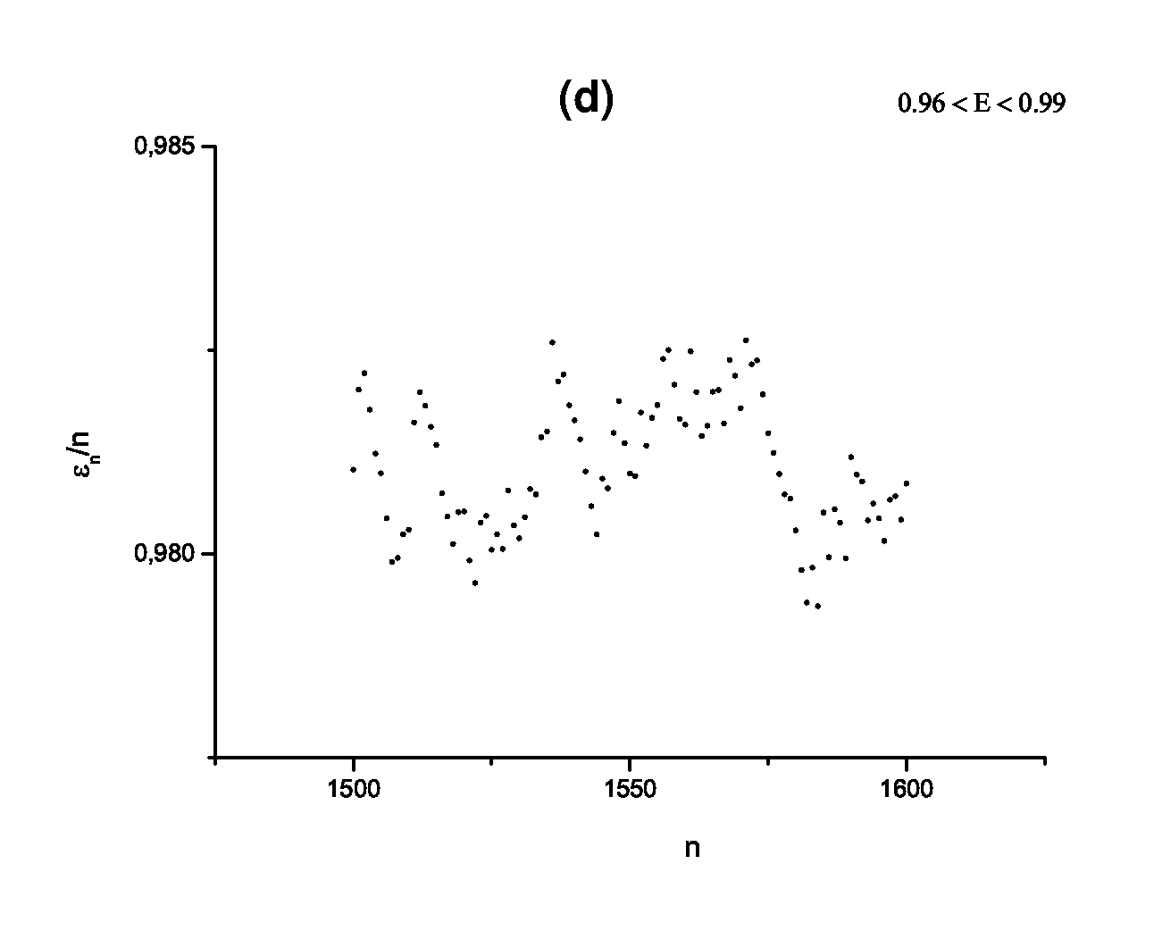
Figure 6.12: Accuracy estimation for the unfolding with (6.20) in the spectrum of lower umbilic catastrophe $D_{5}$ potential (2.4) for $0.50<E<0.56$(a), $0.60<E<0.66$(b), $0.93<E<0.96$(c), $0.93<E<0.99$(d).

Therefore in potentials with multiple local minima, the smoothed semiclassical state number function can be calculated as the sum of partial contributions from each local minimum. In the case of mixed state it gives a convenient way to estimate the relative density of states of regular and chaotic type.

The second reason for disagreement between Berry-Robnik-Bogomolny distribution and actual numerical data is common for all potential systems (excluding uniform potentials like the coupled quartic oscillator one (5.22)), and it consists of the fact that in smooth potential systems the classical chaoticity measure essentially changes with energy; therefore upper and lower levels in sufficiently long spectral series will correspond to different relations of regular and chaotic components, while all known theoretical distribution functions assume the relation to be constant. It forces us to consider spectral series that are sufficiently narrow in energy, and this makes levels statistics even poorer.

Finally, the specific feature of $D_{5}$ potential, which it shares with $D_{7}$, Barbanis and Hénon–Heilis potential, consists of the fact that in all the above mentioned potentials the discrete energy spectrum, strictly speaking, is absent. It is due to the fact that all those models allow infinite motion for all energies. Nevertheless many researchers discuss spectral fluctuations in such systems, implying the spectrum of quasistationary states, localized in the corresponding potential well and extremely slowly decaying due to tunneling into the continuous spectrum. Any numerical calculation of such states practically contains implicit reformulation of the original model in order to make it more correct from the point of view of quantum mechanics. The quasi-stationarity of such states becomes especially manifest near the saddle energies — the most interesting energy region for investigation of the mixed state.

The FNNS for $D_{5}$ potential obtained for narrow energy intervals are presented in Fig.6.13 in normal and in Fig.6.14 in logarithmic scale, and the corresponding cumulative distributions are presented in Fig.6.15 in $W$-representation and on Fig.6.16 in $T$-representation. Regardless of the rather poor statistics (only $100$ levels in each spectral series), we should note quite good qualitative agreement between the fitting parameters of the Brody and the Berry-Robnik-Bogomolny distributions on the one hand and relative phase volumes of regular and chaotic regions in classical phase space (see the Poincaré surfaces of section on Fig.6.17).

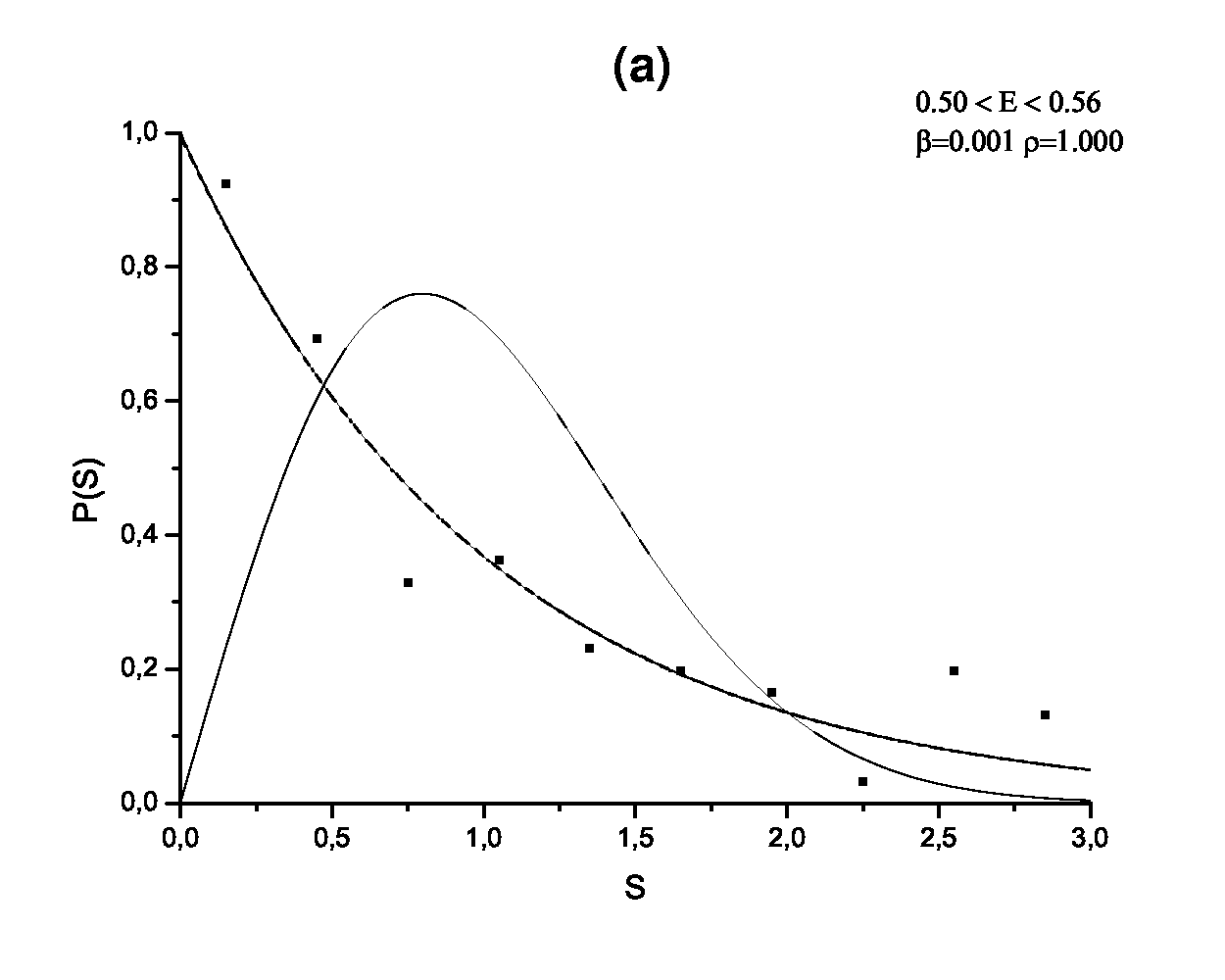
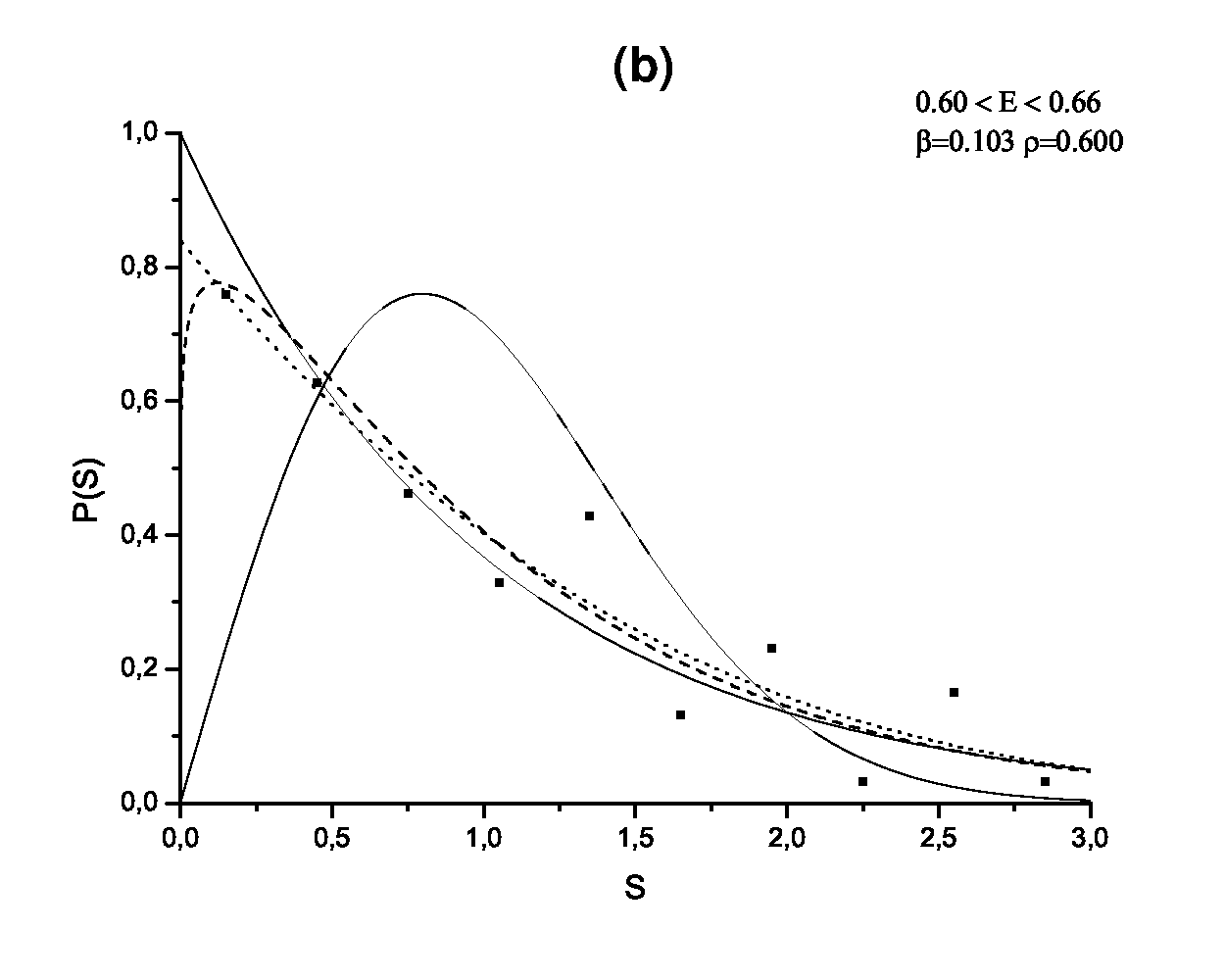
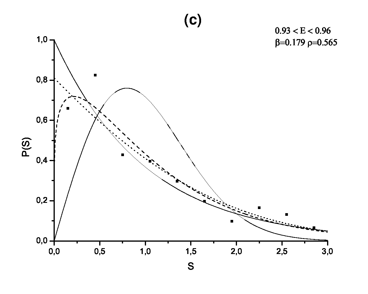
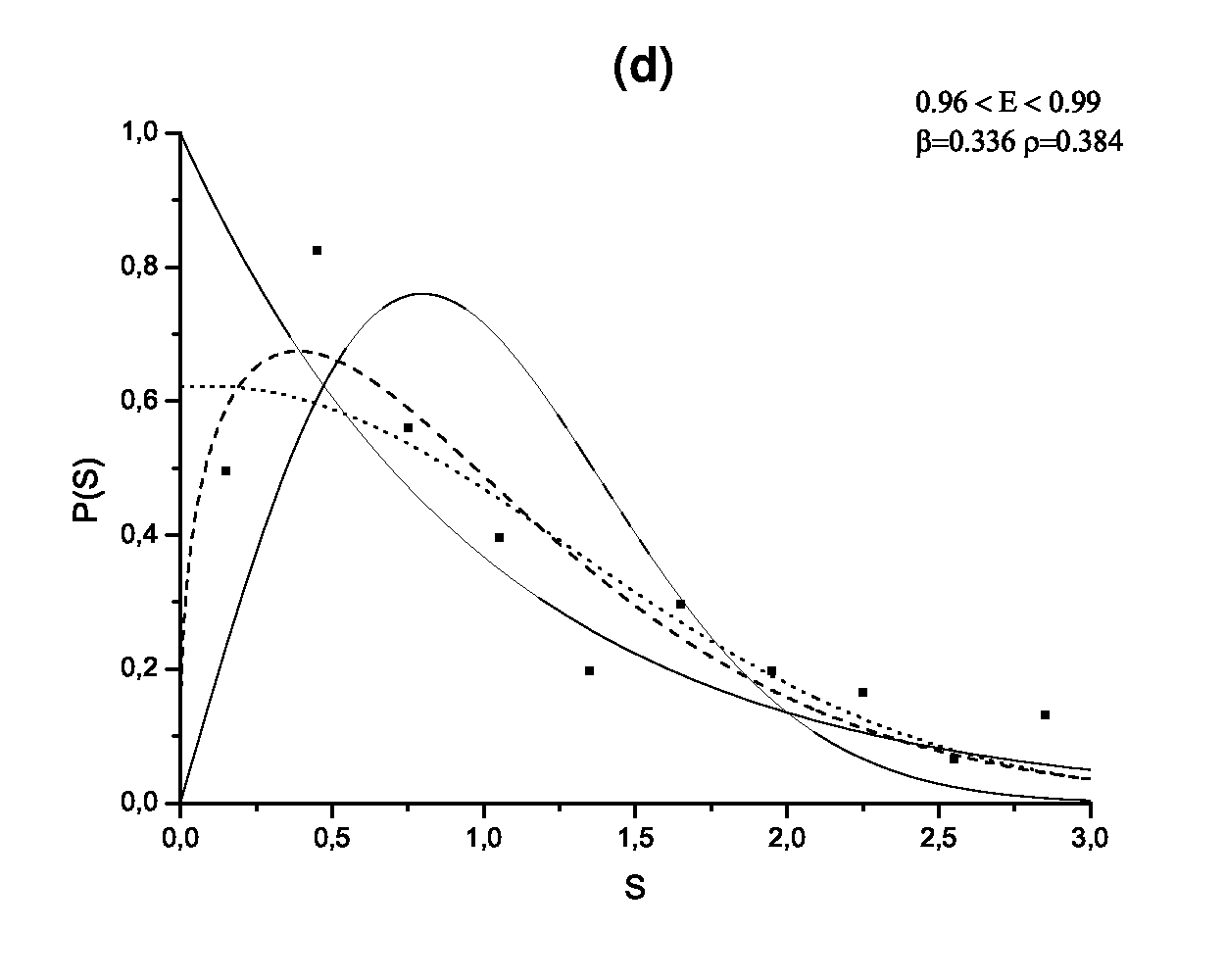
Figure 6.13: FNNS for lower umbilic catastrophe $D_{5}$ potential (2.4) for $0.50<E<0.56$(a), $0.60<E<0.66$(b), $0.93<E<0.96$(c), $0.93<E<0.99$(d). Points represent numerical data, solid lines — Poisson (6.8) and Wigner (6.9) distributions, dashed and dotted lines — the best fits by the Brody (6.10) and the Berry-Robnik-Bogomolny (6.11) distributions respectively.

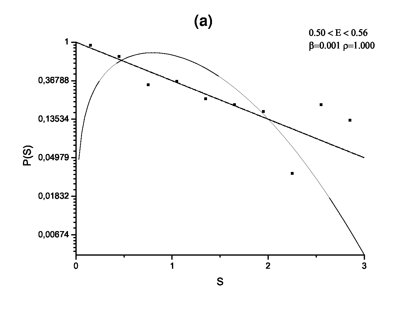
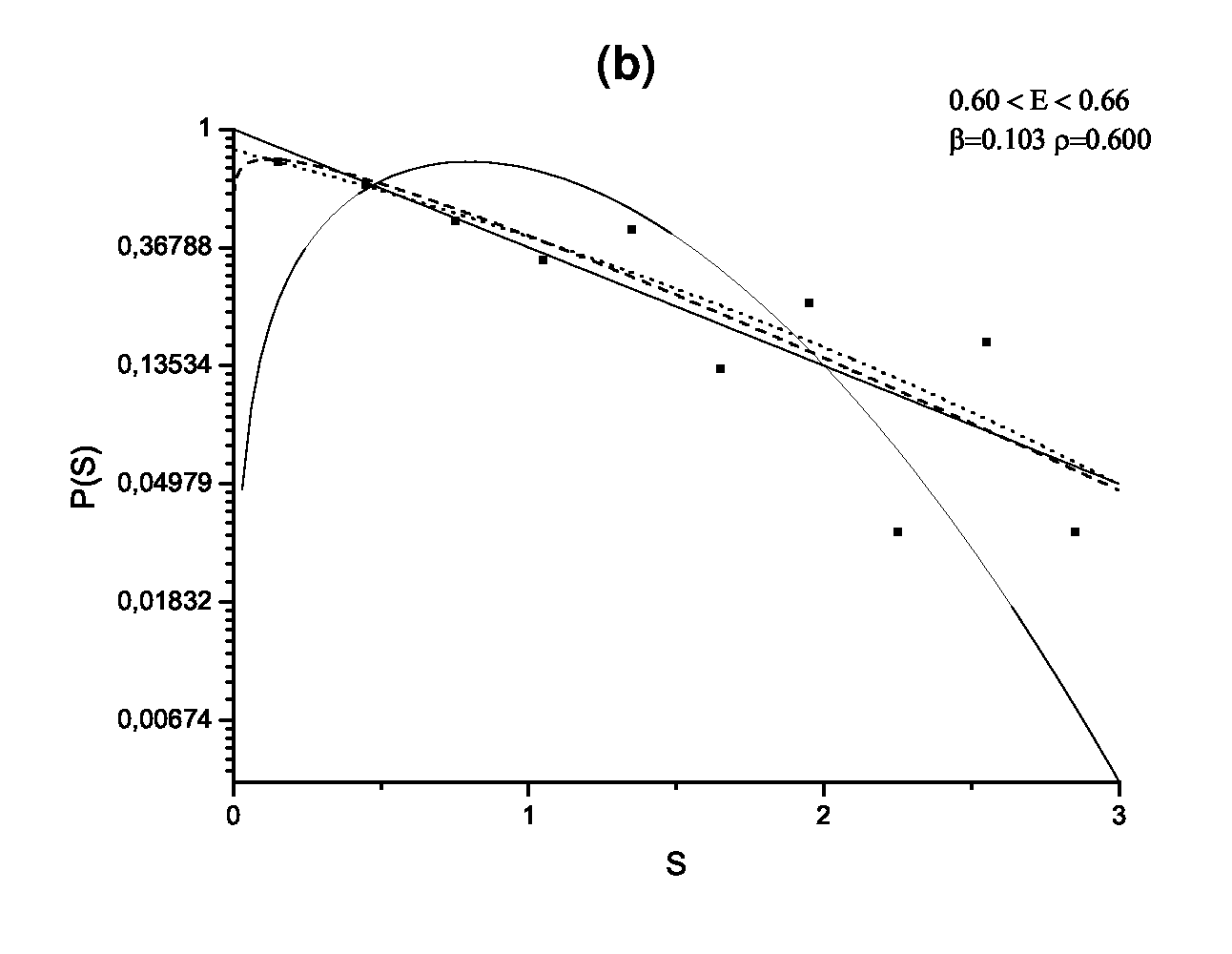
Figure 6.14: The same as on Fig.6.13 but in logarithmic scale.

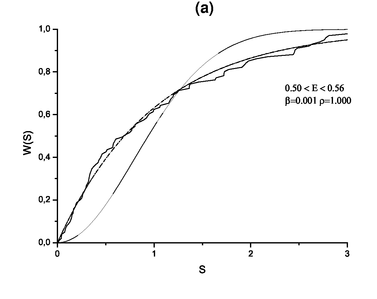
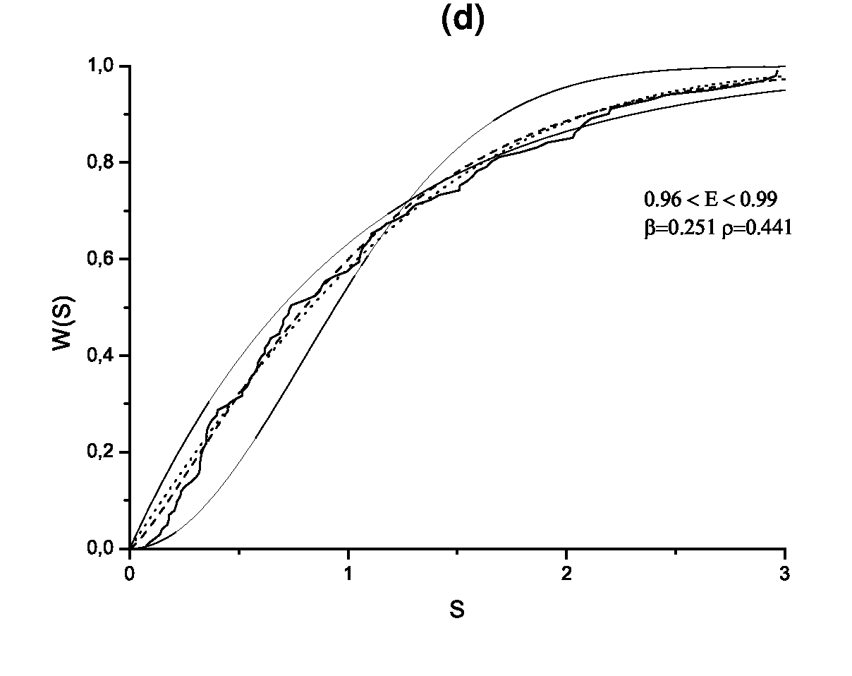
Figure 6.15: Cumulative FNNS for lower umbilic catastrophe $D_{5}$ potential (2.4) for $0.50<E<0.56$(a), $0.60<E<0.66$(b), $0.93<E<0.96$(c), $0.93<E<0.99$(d). Points represent numerical data, solid lines — Poisson and Wigner (6.16) distributions, dashed and dotted lines — the best fits by by Brody and Berry-Robnik-Bogomolny (6.15) distributions respectively.

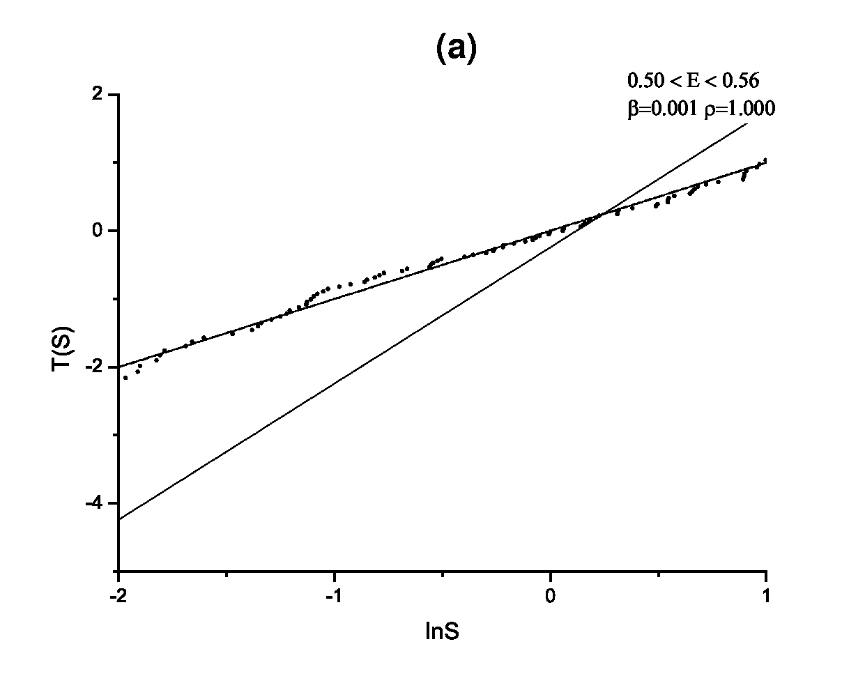
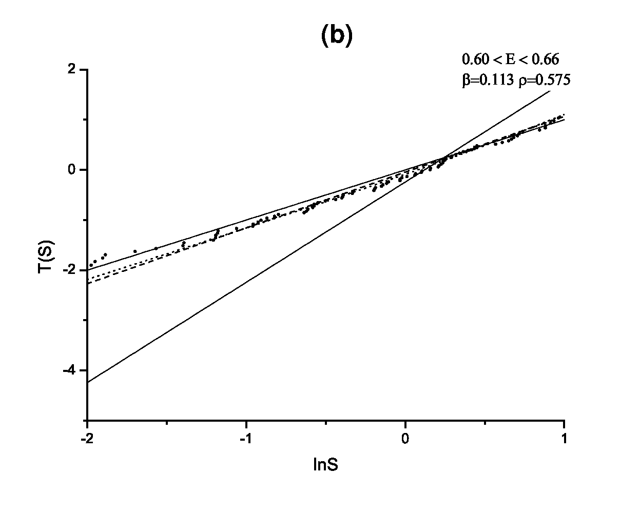
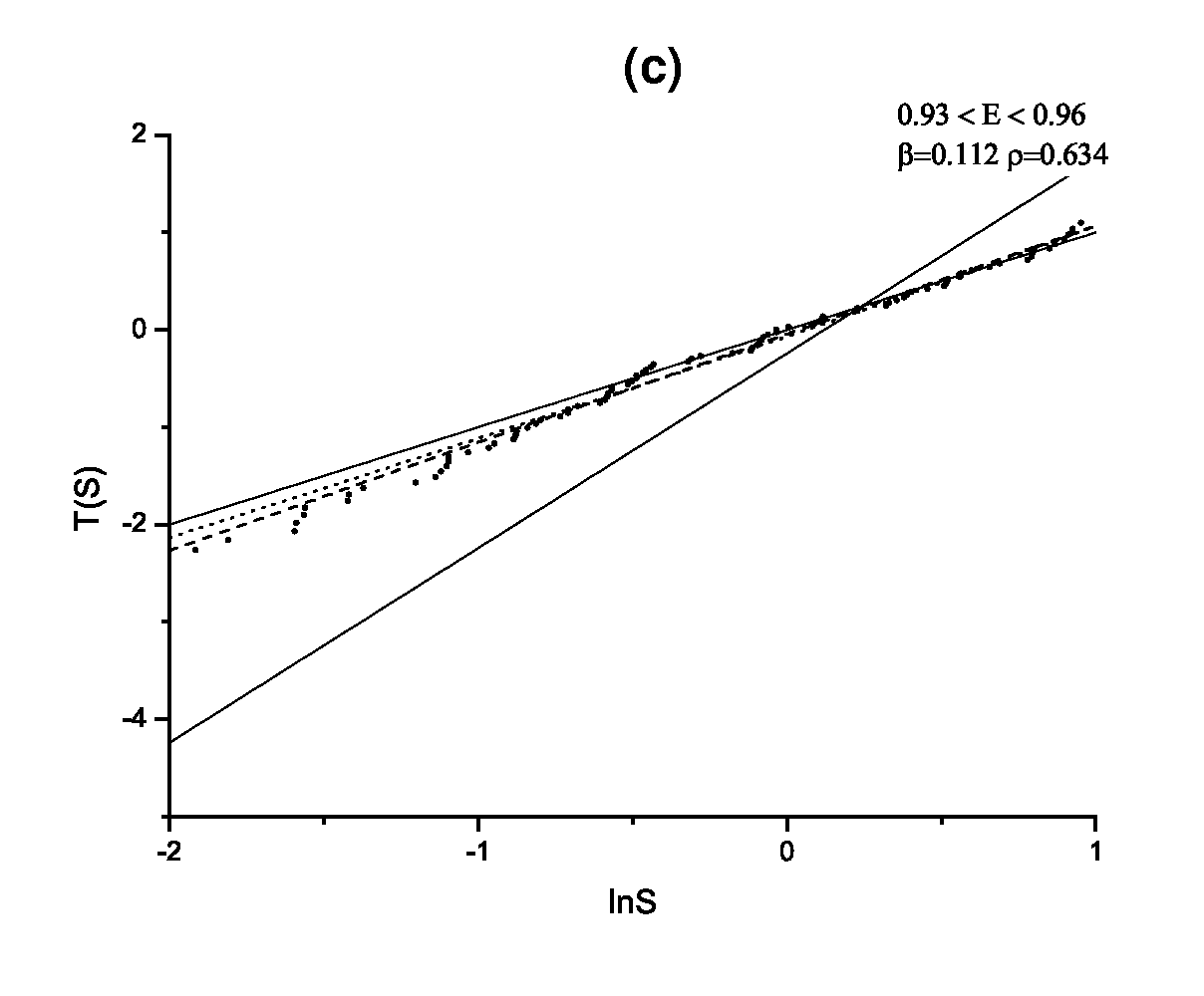
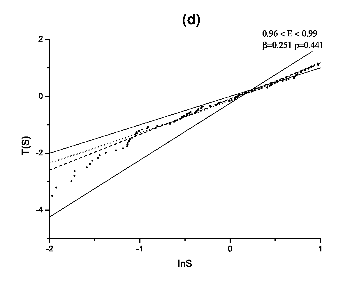
Figure 6.16: Cumulative FNNS in the $T$-representation for lower umbilic catastrophe $D_{5}$ potential (2.4) for $0.50<E<0.56$(a), $0.60<E<0.66$(b), $0.93<E<0.96$(c), $0.93<E<0.99$(d). Points represent numerical data, solid lines — Poisson and Wigner (6.18) distributions, dashed and dotted lines — the best fits by the Brody (6.17) and the Berry-Robnik-Bogomolny (6.19) distributions respectively.

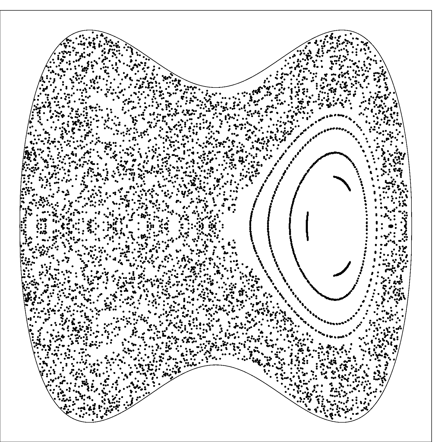
Figure 6.17: Poincaré surfaces of section for lower umbilic catastrophe $D_{5}$ potential (2.4) for $E=0.5$(a), $E=0.6$(b), $E=0.9$(c), $E\lesssim 1$(d). Solid lines limit classically allowed region of the phase space.

As we can see, the Brody distribution gives better agreement than the Berry-Robnik-Bogomolny distribution with numerical FNNS distributions in the $D_{5}$ potential. It is manifested both in the accuracy for each energy interval separately and in the variation of $\beta$ parameter with energy growth; in contrast to the $\rho$ parameter in the fitting by Berry-Robnik-Bogomolny distribution, it grows monotonously with growth of chaoticity measure of classical motion and coincides in order of magnitude with the relative volume of the classical chaotic component.

The unsatisfactory applicability of Berry-Robnik-Bogomolny the distribution for description of spectral fluctuations in the mixed state is explained first of all by insufficient quasiclassicality of the considered states. However a more important reason for such disagreement of theory and experiment appears to be connected with the specific features of energy spectra in the mixed state. It lies in the fact that that many of the energy levels in the potentials with multiple local minima actually appear to be very close to those energy levels that correspond to each local minimum separately — neglecting the small influence of other minima. Those levels are in their turn very well described by spectral series obtained in the harmonic oscillator approximation, especially for not too high energies. In the case of the mixed state especially close to the harmonic oscillator levels appear to be those states that correspond to minima with regular motion in the classical limit.

In $D_{5}$ potential harmonic approximation is given by a mixture of two spectral series of two-dimensional harmonic oscillator levels with eigenfrequencies

$$\omega_{x}=2$$

$$\omega_{y}^{(R,C)}=2\sqrt{1\pm\frac{1}{\sqrt{2}}}$$

where the eigenfrequencies $\omega_{y}^{(R,C)}$ are different for regular and chaotic local minima. Fig.6.18 demonstrates unexpectedly good agreement (in the limits of $1\%$ of mean level spacing for not too high energies) between the harmonic approximation and actual energy levels in the $D_{5}$ potential, and this agreement is better for the regular minimum.

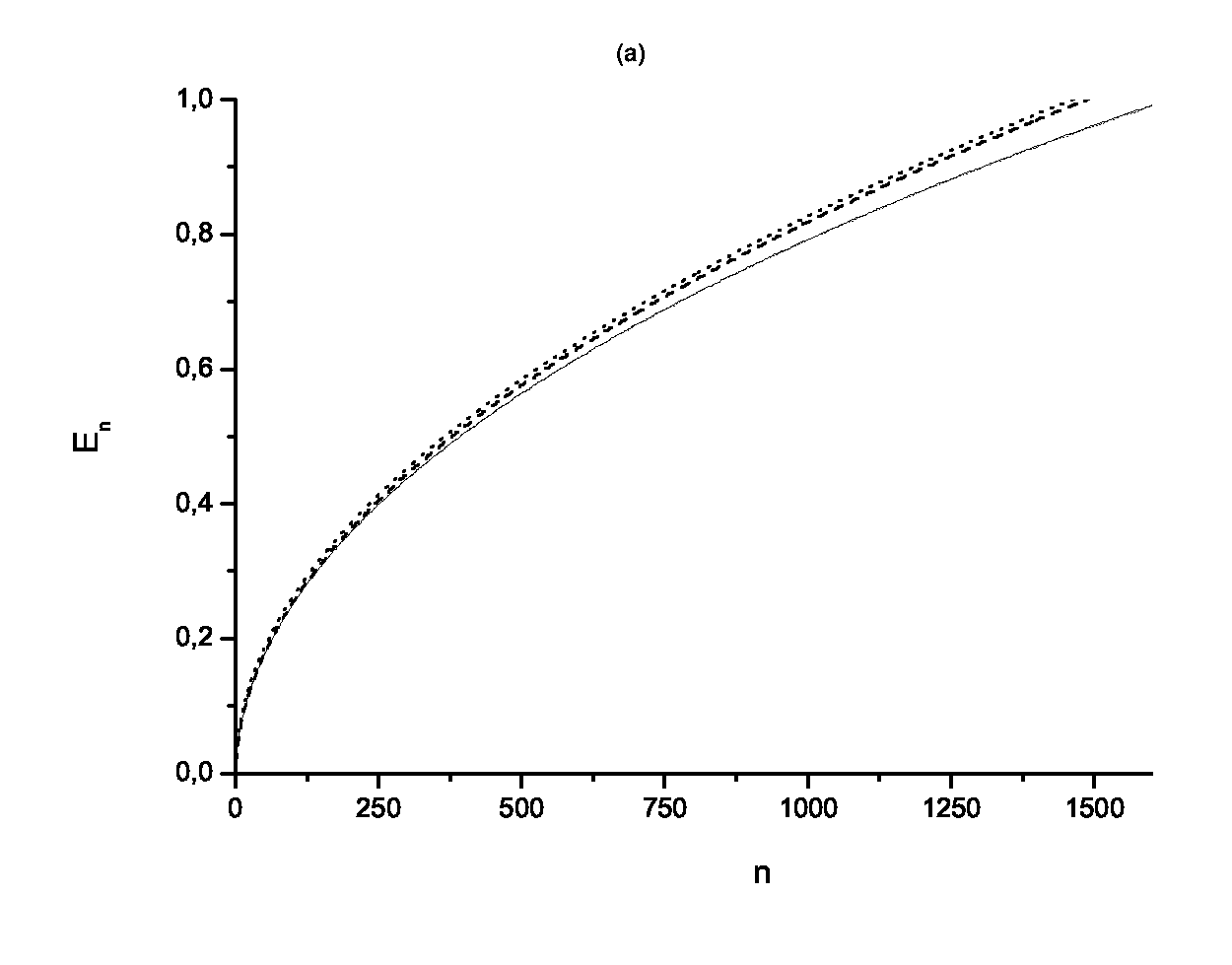
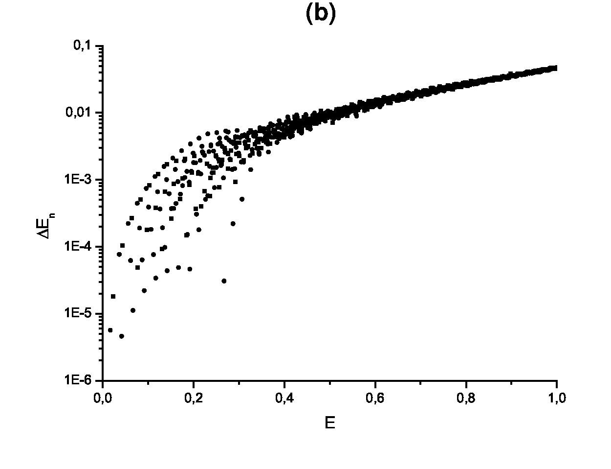
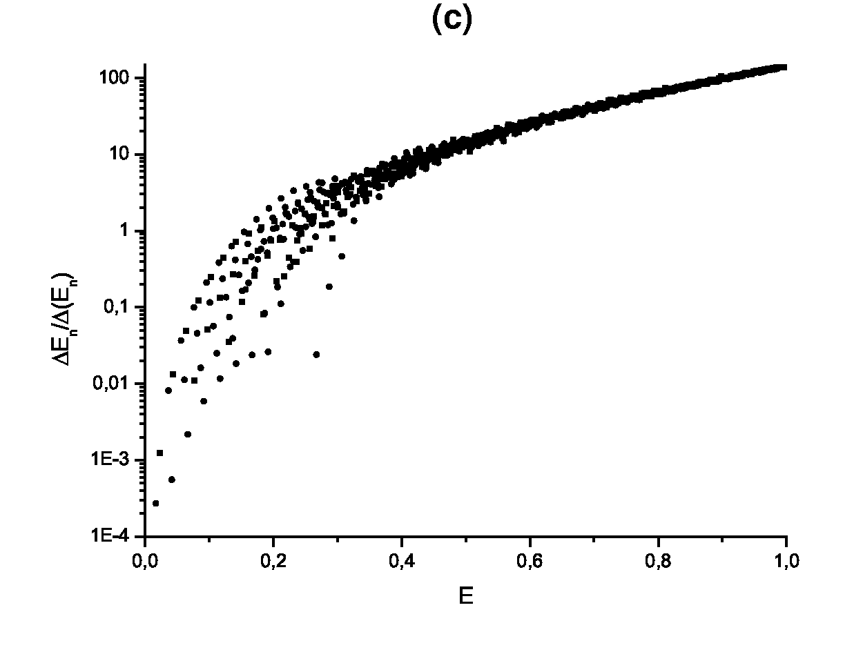
Figure 6.18: Energy levels of lower umbilic catastrophe $D_{5}$ potential (2.4): (a) numerically exact spectrum (solid line), harmonic oscillator (dashed line) and the semiclassical (dotted line) approximations; (b) absolute value of difference between the numerically exact energy levels and harmonic oscillator approximation; (c) absolute value of deviance of numerically exact energy levels from the harmonic oscillator approximation referred to mean level spacing.

Such proximity of the considered spectrum to the harmonic one automatically implies also the mutual proximity of corresponding FNNS distributions. As is well known, FNNS distribution for the harmonic oscillator has a pathological nature — it does not have any universal form, and, therefore, is not described by any of the known distribution functions. Fig.6.19-6.23 present the results of analysis of spectral fluctuations in the harmonic oscillator approximation in lower umbilic catastrophe $D_{5}$ potential (2.4) for chaotic and regular minima separately, and also for a spectrum obtained by mixing of spectral series of both minima.

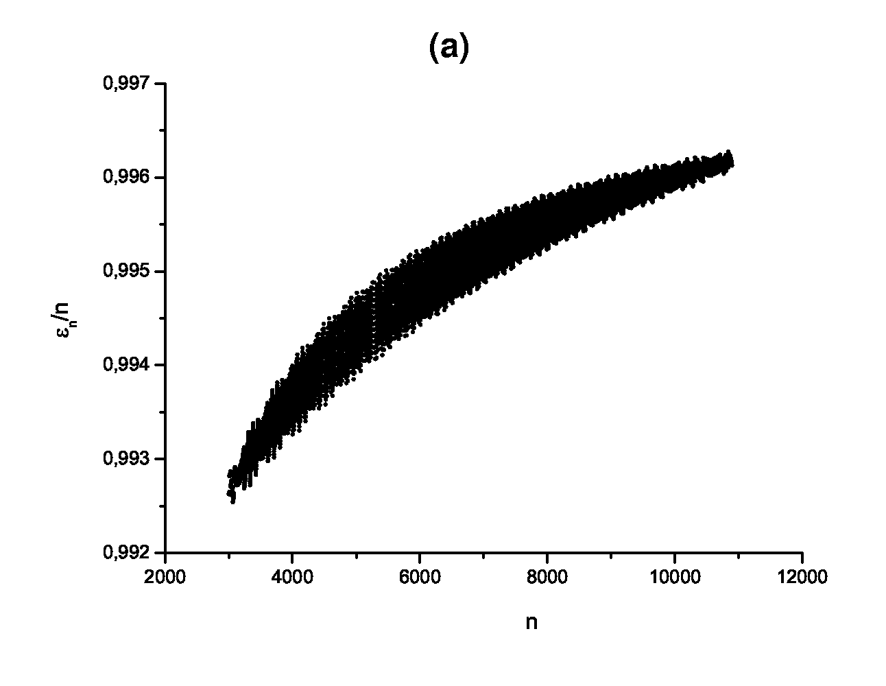
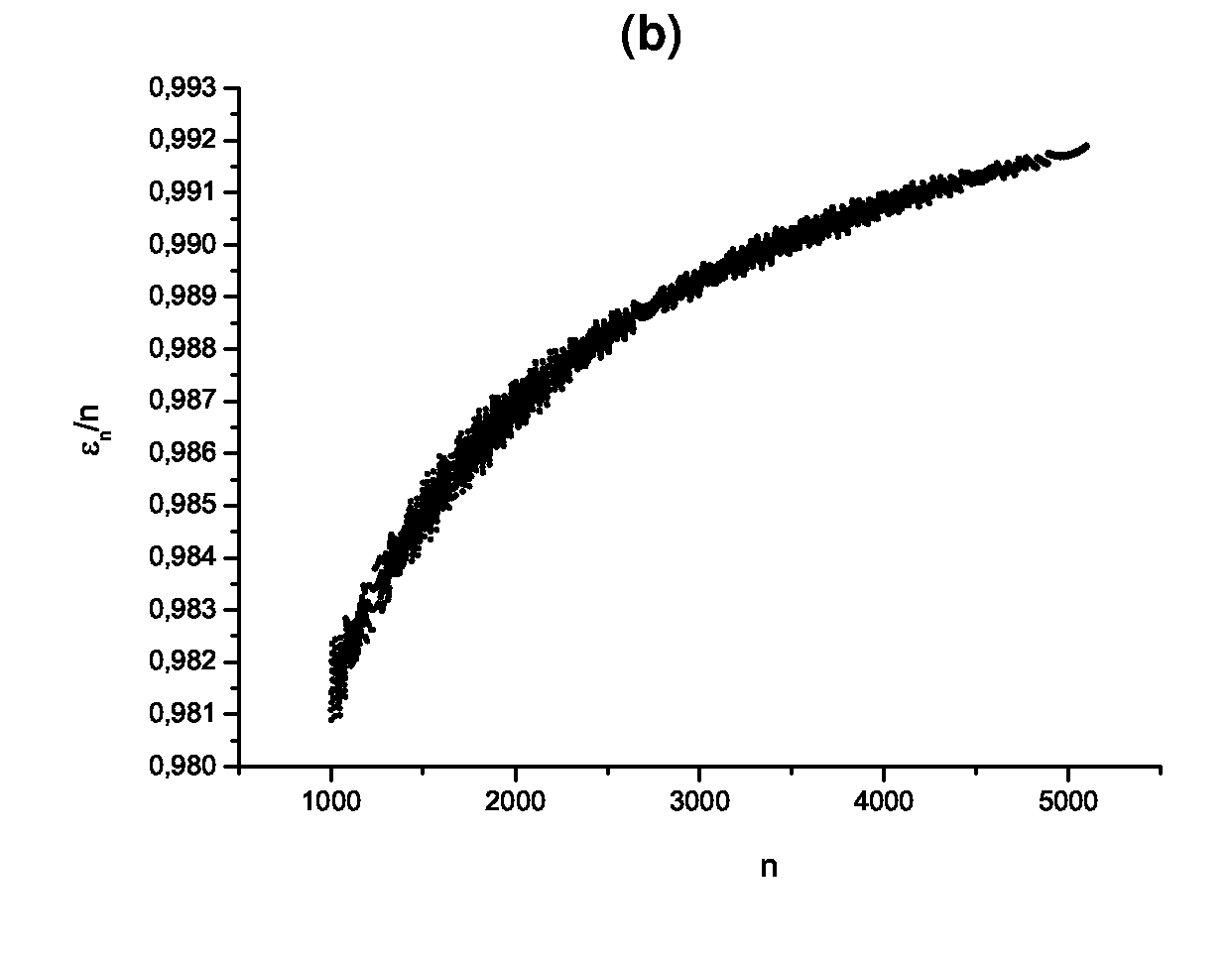
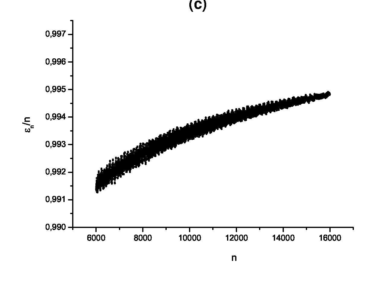
Figure 6.19: Accuracy estimation for the spectrum unfolding of harmonic approximation in lower umbilic catastrophe $D_{5}$ potential (2.4): (a) for chaotic minimum ($x<0$); (b) for regular minimum ($x>0$);(c)for both minima together.

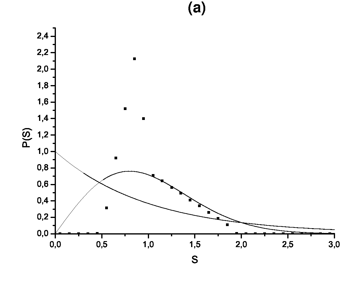
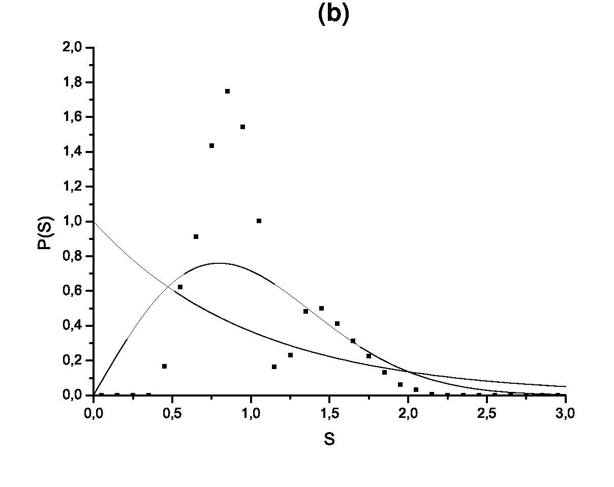
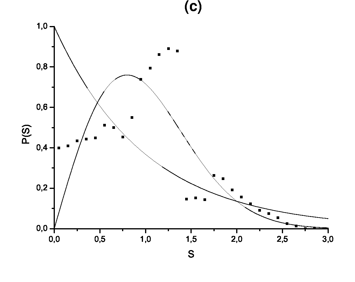
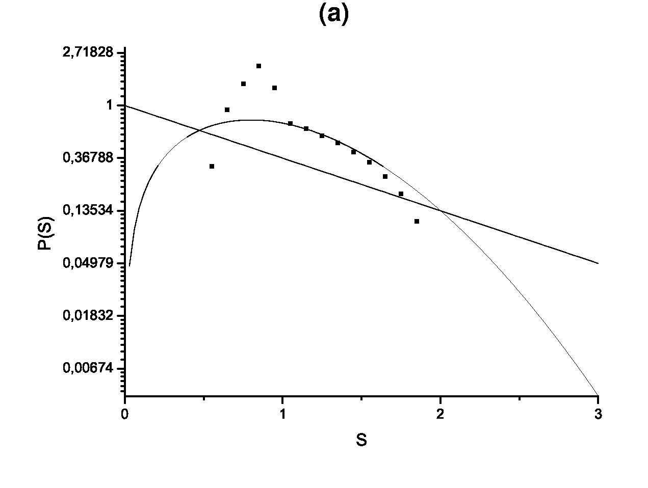
Figure 6.20: FNNS for harmonic approximation in lower umbilic catastrophe $D_{5}$ potential (2.4): (a) for chaotic minimum ($x<0$); (b) for regular minimum ($x>0$);(c)for both minima together. Points represent numerical data, solid lines — Poisson (6.8) and Wigner (6.9) distributions.

Figure 6.21: The same as Fig.6.21 but in logarithmic scale.

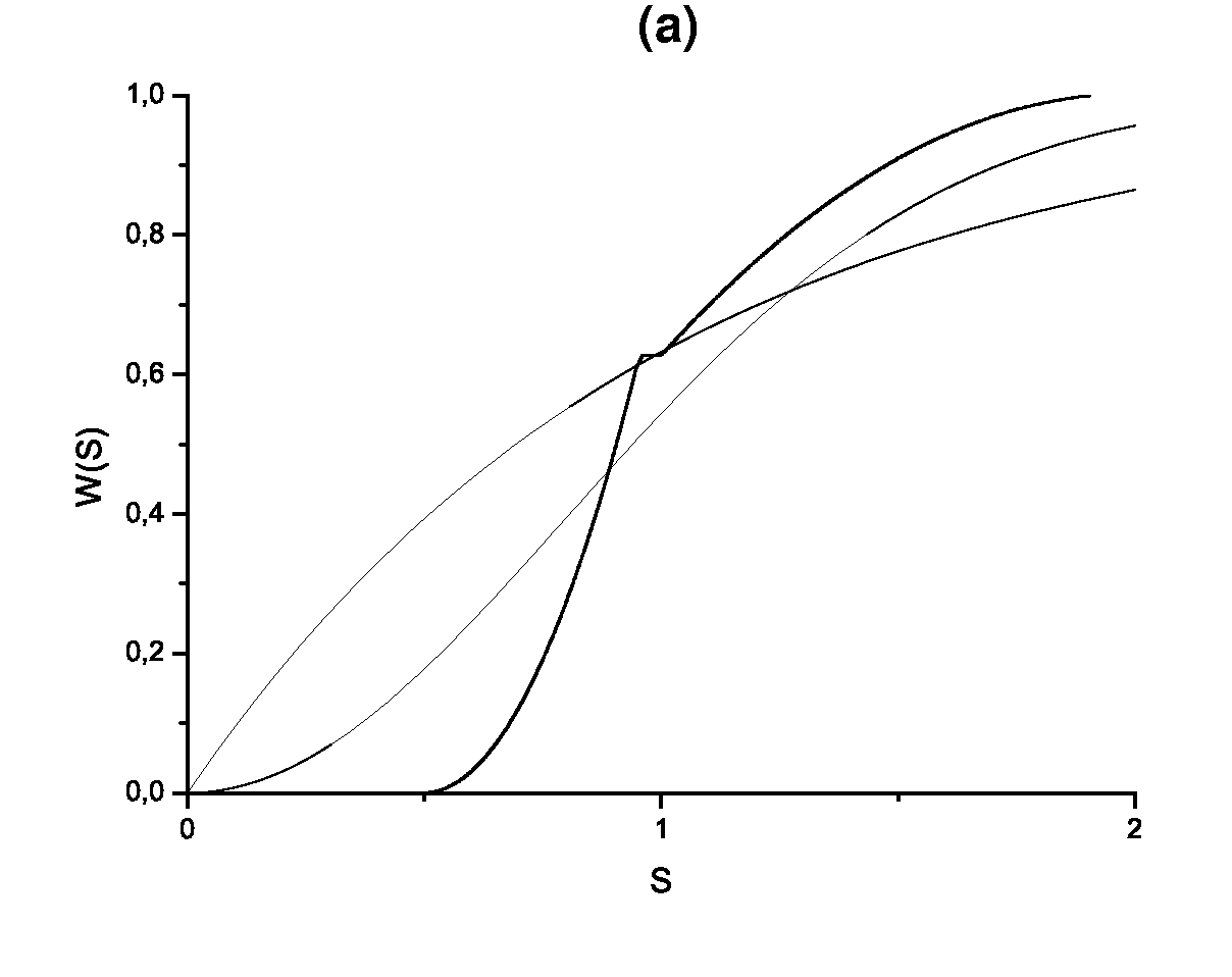
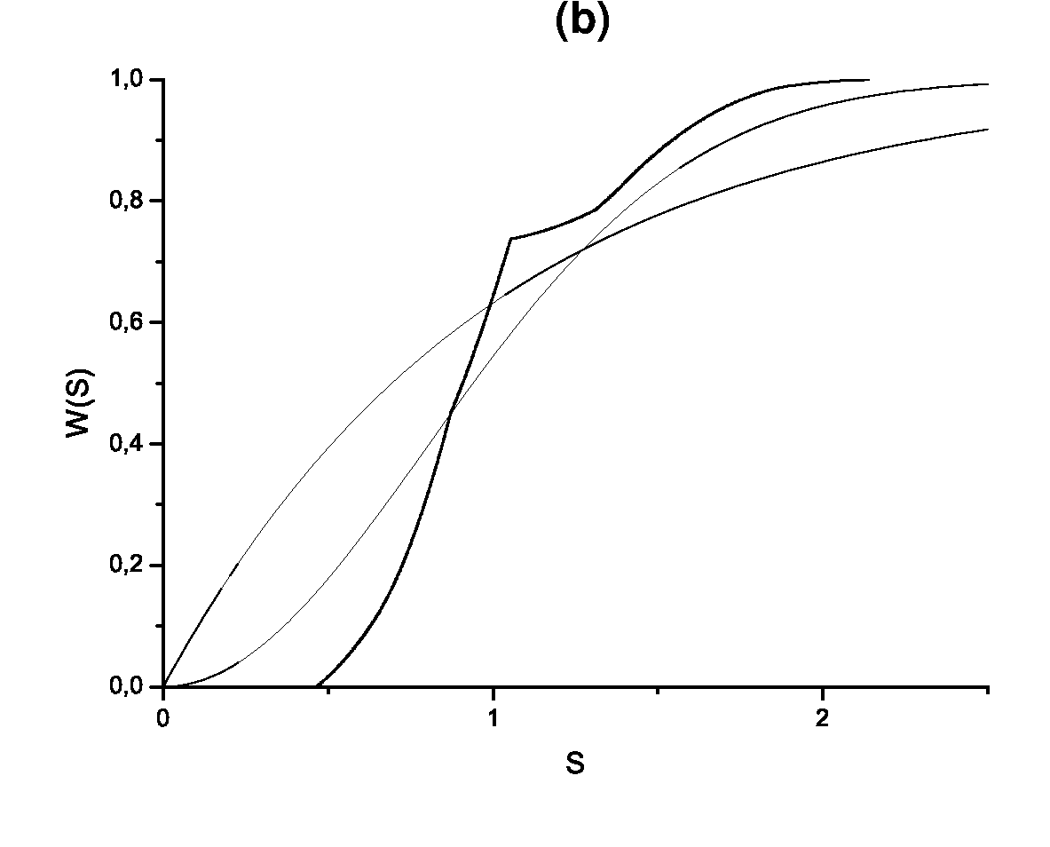
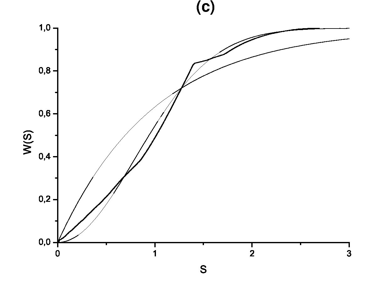
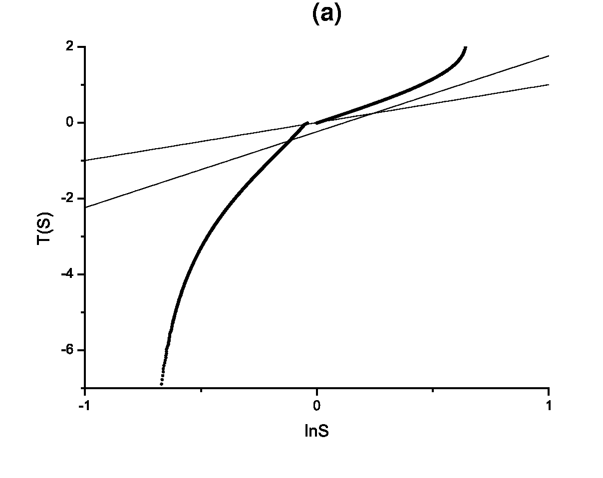
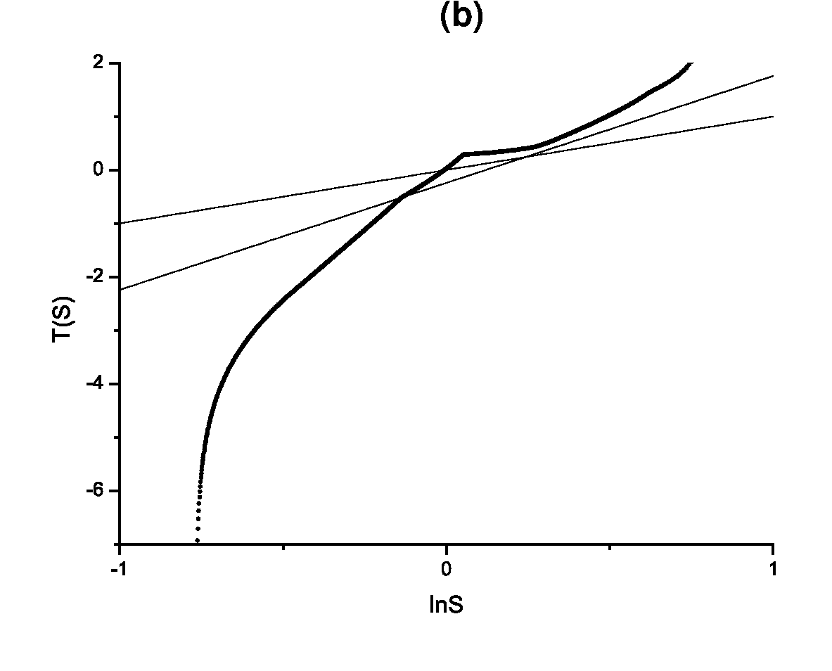
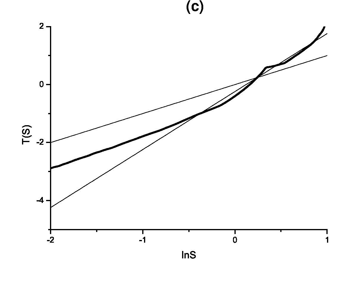
Figure 6.22: Cumulative FNNS for harmonic approximation in lower umbilic catastrophe $D_{5}$ potential (2.4): (a) for chaotic minimum ($x<0$); (b) for regular minimum ($x>0$);(c)for both minima together. Points represent numerical data, solid lines — Poisson and Wigner (6.16) distributions.

Figure 6.23: Cumulative FNNS for harmonic approximation in lower umbilic catastrophe $D_{5}$ potential (2.4) in the $T$-representation: (a) for chaotic minimum ($x<0$); (b) for regular minimum ($x>0$);(c)for both minima together. Points represent numerical data, solid lines — Poisson and Wigner (6.18) distributions.

The FNNS for harmonic oscillator spectrum has multiple maxima, determined by its eigenfrequencies. Therefore the FNNS distribution for the harmonic approximation spectrum in the mixed state has many maxima, corresponding to all eigenfrequencies of the approximations. That dependence of the FNNS distribution form on the eigenfrequencies of the system is the main reason for the pathological character of level fluctuations in the harmonic oscillator spectrum. In the case of the mixed state, energy levels, close to the harmonic ones, will give essential (and pathological) contribution to FNNS distribution. The theoretical distribution function, accounting for such a contribution, should be constructed as mixed statistics from components of three types: not only chaotic or regular, but also harmonic ones, carrying pathological spectral fluctuations. The construction of such a distribution function is a problem for the future.

6.3 Other statistical characteristics of spectra — $1/f$-noise

FNNS is far from being the unique tool for investigation of quantum manifestations of classical stochasticity in the structure of quantum energy spectra in the systems whose classical analogues demonstrate chaos. One of the alternative approaches [61] to quantum chaos description is based on traditional time series analysis methods. Let us consider the energy spectrum as a discrete signal, and a sequence of $N$ energy levels as a time series. Let us characterize the spectral fluctuations with the $\delta_{n}$-statistics, defined as the following:

$$\delta_{n}=\sum\limits_{i=1}^{n}(s_{i}-\langle s\rangle)=\sum\limits_{i=1}^{n}w_{i},$$

where index $n$ runs from $1$ to $N-1$. Quantities $w_{i}$ give the fluctuation of the $i$-th spacing between neighboring levels with respect to its mean value $\langle s\rangle=1$. We assume that the standard procedure of spectrum unfolding (6.6) was made in advance, i.e. the original spectrum was mapped into another spectrum $(E_{i}\rightarrow\varepsilon_{i})$ with mean level spacing equal to unity, then $s_{i}=\varepsilon_{i+1}-\varepsilon_{i}$, $i=1,\ldots,N$.

Our goal is to study transformation of the above introduced characteristics $\delta_{n}$ in transition from regular systems to chaotic ones. One uf the useful methods is to calculate the power spectrum $S(k)$ of the discrete and finite series $\delta_{n}$ according to the following:

$$S(k)=|\hat{\delta}_{k}|^{2}$$

where $\hat{\delta}_{k}$ is the Fourier transform of $\delta_{n}$,

$$\hat{\delta}_{k}=\frac{1}{\sqrt{N}}\sum\limits_{n}\delta_{n}e^{-\frac{2\pi ikn}{N}}$$

and $N$ is the number of terms in the series.

As an example of a chaotic system authors [61] have chosen the atomic nucleus at high excitation energies, where level density is very high. In order to obtain the energy spectrum the authors performed calculations in the shell model with realistic interaction reproducing the experimental data well. Hamiltonian matrices for differen values of angular momentum were diagonalized and the unfolding operation was accurately done for the obtained spectra. After that the authors selected sets from $256$ consecutive levels each with the same $J^{\pi},T$ from high level density regions. In order to characterize the statistical properties of the signal $\delta_{n}$ the authors calculated the ensemble average of its power spectrum. The averaging was performed in order to decrease the statistical fluctuations (errors) and to clarify the general tendency. Average $\langle S(k)\rangle$ was calculated over the ensemble of $25$ sets.

Fig.6.24 represents the results for a typical stable $sd$ shell of ²⁴Mg nucleus (the spectrum was obtained by diagonalization of a $2000\times 2000$ martrix) and for a very exotic ³⁴Na nucleus — $sd$ proton shell and $pf$ neutron one ($5000\times 5000$ matrix diagonalization). It can be clearly seen that the power spectrum for $\delta_{n}$ is close to power law. It is possible to assume simple functional form

$$\langle S(k)\rangle\sim\frac{1}{k^{\alpha}}.$$

The least squares fit gives $\alpha=1.11\pm 0.03$ for ³⁴Na $\alpha=1.06\pm 0.05$ for ²⁴Mg. A natural question arises: does there exist an universal relation between peculiarities of quantum spectrum, connected with the character of classical motion, and the power spectrum of $\delta_{n}$ fluctuations?

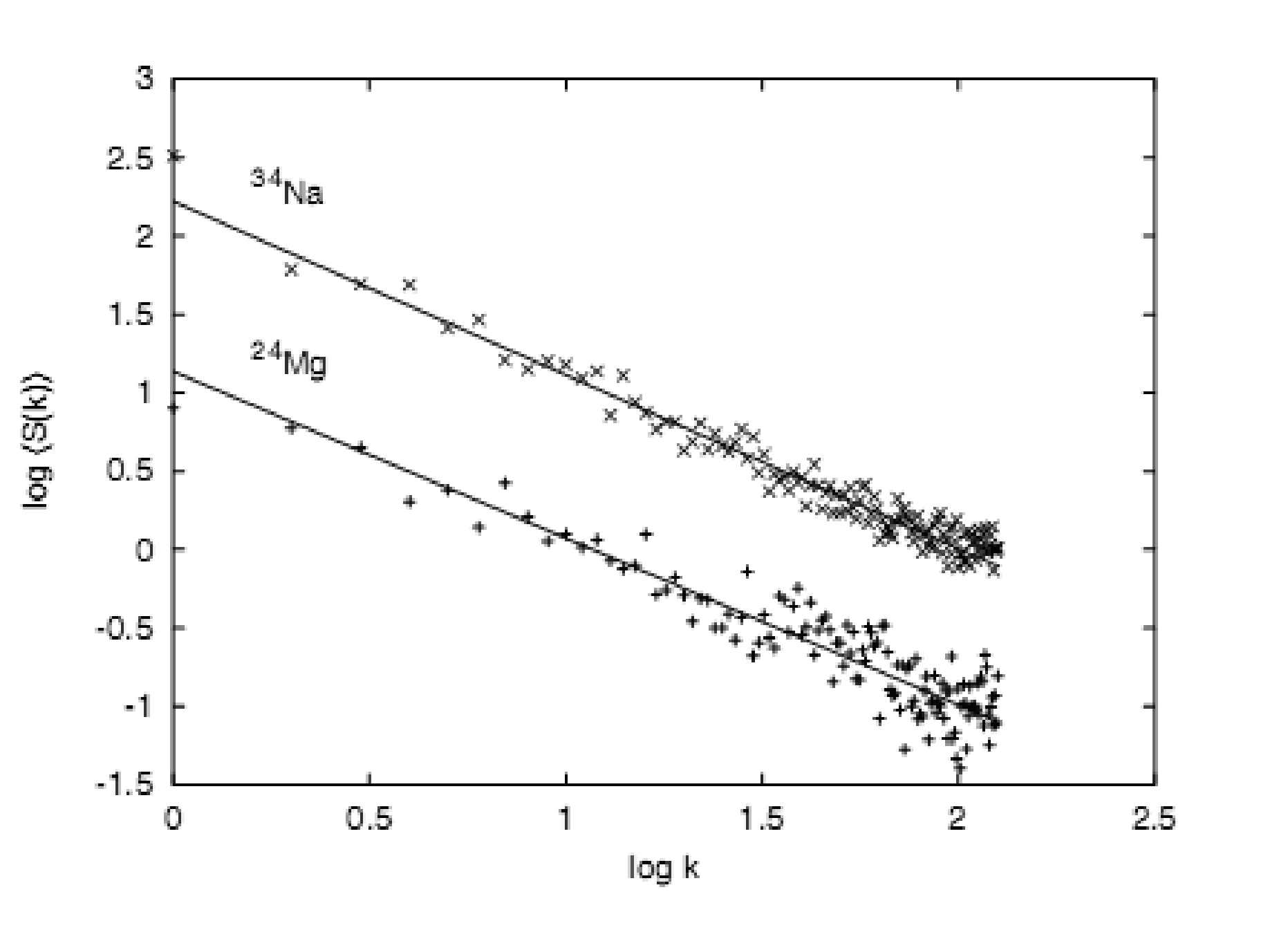
Figure 6.24: Average power spectrum of the $\delta_{n}$ function for ²⁴Mg and ³⁴Na, using $25$ sets of $256$ levels from the high level density region. The plots are displaced to avoid overlapping.

Probably the simplest way to answer that question is to compare $\delta_{n}$ and $\langle S(k)\rangle$ for level sequences corresponding to Poissonian statistics with the results for different random matrices ensembles. Fig.6.25 presents the $\delta_{n}$ signal for the Poissonian and GOE spectra of dimensionality $1000$. It is clear that the signals are absolutely different. We compare them with discrete time series $x(t)$ corresponding to power spectra $1/k$ and $1/k^{\alpha}$. The proximity of the $\alpha=2$ time series to the Poissonian spectrum and of $\alpha=1$ — to to GOE one is evident.

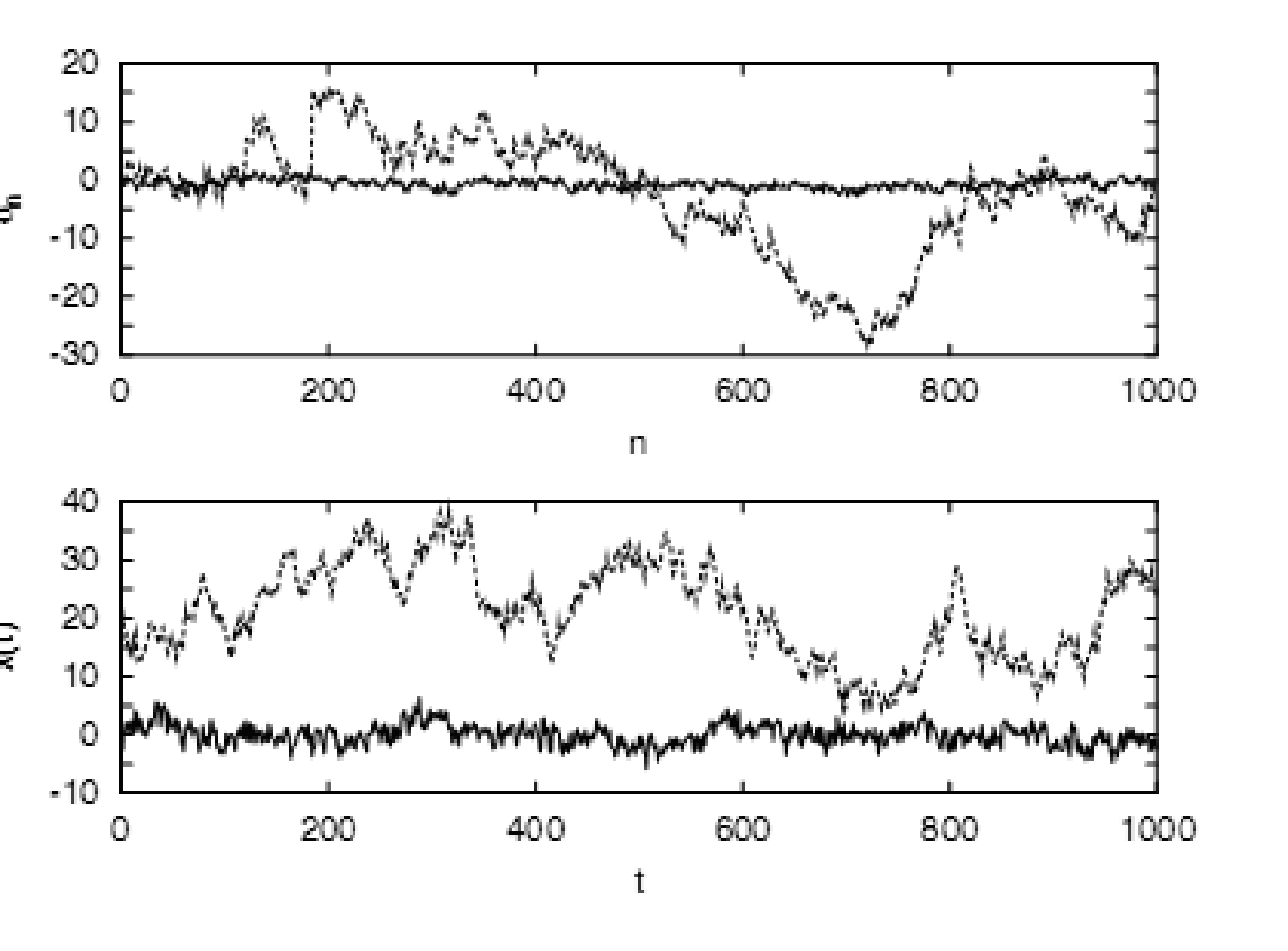
Figure 6.25: Comparison of the $\delta_{n}$ function for Poisson (dashed line) and GOE spectra (solid line), with a standard time series $x(t)$ with $1/k^{\alpha}$ power spectrum, for $\alpha=2$ (dashed line) and $\alpha=1$ (solid line).

In order to calculate $\langle S(k)\rangle$ there were built $30$ different matrices of dimensionality $1000\times 1000$ for random matrix ensembles of different types mentioned above. Fig.6.26 presents the results of the calculations in double logarithmic scale. In all the considered cases the general tendency is linear with the exception of the very high energy region, where some deviations are observed which are probably due to the finiteness of dimensionality of the considered matrices. Ignoring frequencies with $k>2.2$, the fitting gives $\alpha=1.99$ for Poissonian spectrum with uncertainty about $2\%$.

In contrast to the last example, the GOE of high dimension matrices is usually considered as a paradigm for the chaotic quantum spectrum. It demonstrates level-level correlations on all scales. The same refers also to unitary (GUE) and simplectic (GSE) ones, but with increasing level repulsion rate.

Power spectra of $\delta_{n}$ for all the three ensembles are presented on Fig.6.26. For the exponents we obtained the following values: $\alpha_{GOE}=1.08$, $\alpha_{GUE}=1.02$, $\alpha_{GSE}=1.00$. All three ensembles agree with the same power law $\alpha\simeq 1$. It is evident that the power spectrum $\langle S(k)\rangle$ behaves as $1/k^{\alpha}$ both for regular and chaotic spectra, but level correlations decrease from limiting $\alpha=2$ for a regular uncorrelated spectrum to the minimal value $\alpha=1$ for quantum chaotic systems.

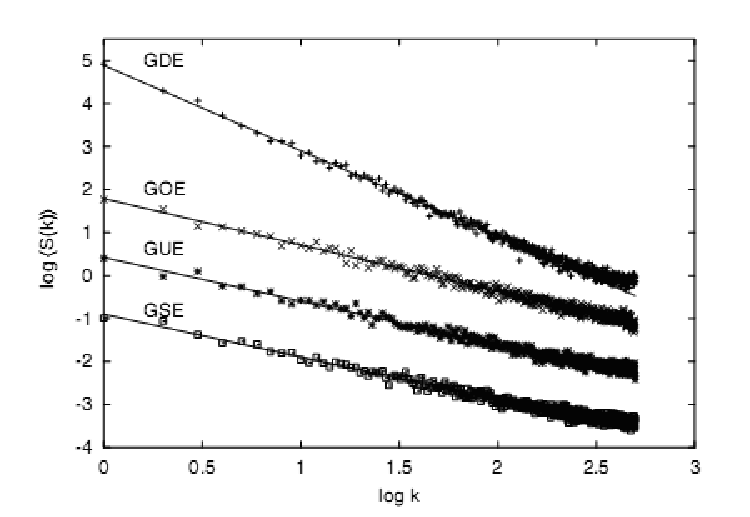
Figure 6.26: Power spectrum of the $\delta_{n}$ function for GDE (Poisson) energy levels, compared to GOE, GUE and GSE. The plots are displaced to avoid overlapping.

The above result for the $\delta_{n}$ statistics power spectrum gives rise to the following hypothesis: energy spectra of chaotic systems are characterized by $1/f$ noise. Let us recall that $1/f$ (flicker noise) was discovered in the 1920s: slow flicks (from which the name comes) of emission capacity of cathode lamps (as a result of current fluctuations) superposed on fast thermal (fraction) current fluctuations. For white noise $S(\omega)=const$ in a wide frequency range, while for the flicker noise $S(\omega)\propto 1/\omega$.

Flicker noise was discovered in many physical and biological systems. A common property of all such systems is the fact that $1/f$ noise is a satellite of stationary irreversible processes: its contribution disappears in the absence of irreversible flows and the system reaches the thermodynamic equilibrium. In reality $1/f$ noise is always weak in the sense that it carries only a small part of average fluctuation squared: the main contribution is due to white noise. But at low frequencies $1/f$ noise may exceed white noise by several orders of magnitude and becomes the main harmful factor for devices that work on such frequencies. An important feature of flicker noise is the increase of its spectral density with frequency decrease, which takes place up to minimal measurable frequencies of about $10^{-7}$ Hertz without any tendency to saturation. Thus the main question is: should one seek for a universal flicker nose mechanism common for all media and systems, or it is better to assume the existence of many flicker noises of different characters. This question is unanswered up to now.

The hypothesis proposed in [61] has several attractive features. The considered properties characterize the chaotic spectrum immediately without reference to properties of other systems (such as random matrices ensembles). It is universal for all types of chaotic system and does not depend on such properties as time reversal invariance and whether spins are integer or half-integer. Also the $1/f$ characteristics unites a rich diversity of quantum chaotic systems from many different fields of science — flicker noise is everywhere! Therefore the energy spectra of chaotic systems demonstrate the same type of fluctuations as many other systems. However there is no indication that $1/f$ noise in spectral fluctuations of quantum systems implies $1/f$ noise in the corresponding classical analogues.

Chapter 7 Signatures of Quantum Chaos in Wave Function Structure

7.1 QMCS in wave functions structure

As we have seen in the previous section, the statistical properties of spectra have been rigidly correlated with the type of classical motion. It is natural to try to discover the analogous correlations in the structure of wave functions, i.e. to assume that the form of the wave function for a semiclassical quantum state depends on whether it is associated with classical regular or chaotic motion. Furthermore it should be pointed out that in the analysis of quantum manifestations of classical stochasticity at the level of energy spectra, the principal role was given to statistical characteristics, i.e., quantum chaos was treated as a property of a group of states. The choice of a stationary wave function of the quantum system, which is chaotic in the classical limit, as the basic object of investigation relates the phenomenon of quantum chaos to an individual state. Joint investigation of both the possibilities is not a contradiction but reflects the universality of the considered phenomenon.

In contrast to spectrum, the form of wave functions depends on the basis on which they are determined. For QMCS studies the following three representations are most often used:

1. The so-called $H_{0}$-representation is the representation of eigenfunctions $\{\varphi_{n}\}$ of the integrable part $H_{0}$ of total Hamiltonian $H=H_{0}+V$. The main objects of investigation in this case are the coefficients of expansion $C_{mn}$ of stationary functions $\psi_{m}$ on basis $\{\varphi_{n}\}$. $H_{0}$-representation is natural in the realization of numerical calculations, as the diagonalization of Hamiltonian $H$ is realized more often in this representation.

2. Coordinate representation $\Psi(\mathbf{x})$ is the most convenient from the point of view of visual clarity as it allows direct comparison with classical motion along the trajectories in coordinate space. Indeed, according to Schnirelman theorem [62], the mean probability density $|\Psi(\mathbf{x})|^{2}$ in the semiclassical limit $\hbar\rightarrow 1$ coincides with projection of micro-canonical distribution onto the coordinate space:

   $$\langle|\Psi(q)|^{2}\rangle\rightarrow\rho_{0}(q)\ with\ \hbar\rightarrow 1$$

   $$\rho_{0}(q)=\frac{\int d^{n}p\delta(E-H(p,q))}{\int d^{n}p^{\prime}d^{n}q^{\prime}\delta(E-H(p^{\prime},q^{\prime}))}$$

   Actually this theorem transmits the correspondence principle on wave functions. What can we expect from the wave function structure basing on the theorem? It is concentration of the probability density in the regions of coordinate space covered by (quasi-)periodic trajectories for regular wave functions, in contrast to almost uniformly smeared probability density for chaotic wave functions.

3. Representation with the help of Wigner functions [63, 64] has a set of properties in common with the classical function of distribution in phase space.

As early as 1977 Berry [65] assumed that the form of the wave function $\psi$ for a semiclassical regular quantum state (associated with classical motion on a $N$-dimensional torus in the $2N$-dimensional phase space) was very different from the form of $\psi$ for an irregular state (associated with stochastic classical motion on all or part of the $(2N-1)$-dimensional energy surface in phase space). For regular wave functions, the average probability density in the configuration space was seen to be determined by the projection of the corresponding quantized invariant torus onto the configuration space, which implies global order. The local structure is implied by the fact that the wave function is locally a superposition of a finite number of plane waves with the same wave number as determined by classical momentum. In the opposite case for chaotic wave functions the averaged (over small intervals of energy and coordinates) $|\psi_{n}|^{2}$ in the semiclassical limit $\hbar\rightarrow 0$ coincides with the projection of the classical micro-canonical distribution onto the coordinate space. Its local structure is spanned by the superposition of infinitely many plane waves with random phases and equal wave numbers. The random phases might be justified by classical ergodicity, and this assumption immediately predicts locally the Gaussian randomness for the probability of amplitude distribution. Such a structure of wave function is in good agreement with the picture of classical phase space: the classical trajectory homogeneously fills the isoenergetic surface in the case of chaotic motion. By contrast, from the consideration of regular quantum state as an analogue of classical motion on a torus, a conclusion should be done about the singularity (in the limit $\hbar\rightarrow 0$) of the wave function near caustics (boundaries of the region of classically allowed motion in a coordinate space).

Berry’s hypothesis was subjected to the most complete test for billiards of different types and, in particular, for a billiard stadium type [66]. The amplitude of a typical wave function of an integrable circular billiard is negligible in the classically prohibited region (from conservation of angular momentum in a circular billiard it should be clear that the arbitrary trajectory is enclosed between the external and a certain internal circle, the radius of which is determined by the angular momentum magnitude) , whereas near the caustics it is maximal. Distribution of $|\psi_{n}|^{2}$ for the case of a stadium billiard, (classical dynamics is stochastic) is strongly distinguished from the integrable case. However, this distribution is not so homogeneous, as we could expect starting from the ergodicity of classical motion [67].

The above considered $R-C-R$ transition represents an attractive possibility to check Berry’s hypothesis for potential systems with a localized instability region. Let us start from the $H_{0}$-representation, or more exactly the representation of linear combinations of wave functions of a two-dimensional harmonic oscillator with equal frequencies

$$\varphi_{k}=\sum\limits_{N,L}C^{k}_{NLj}|NLj\rangle,$$ (7.1)

where

$$|NLj\rangle=\frac{P_{L,j}}{\sqrt{2}}(|N,L\rangle+j|N,-L\rangle),\ j=\pm 1;$$

$$N=0,1,2,\ldots;\ L=N,N-2,\ldots,1\ or\ 0;\ P_{L,j}=j^{Mod(L,3)},$$

$$\langle NLj|N^{\prime}L^{\prime}j^{\prime}\rangle=\frac{1}{\sqrt{2}}2^{\delta_{L,0}}\delta_{NN^{\prime}}\delta_{LL^{\prime}}\delta_{jj^{\prime}}.$$

If we introduce the notion of distributivity of wave function in basis, then the criterion of stochasticity formulated by Nordholm and Rise [68] states that the average degree of distributivity of wave functions arises with the degree of stochastization in the system. It is clear that this criterion is a direct analog of Berry’s hypothesis for $H_{0}$-representation, if one interprets the number of the basis state $i_{NLj}$ as a discrete coordinate. Fig.7.1 qualitatively confirms this criterion. It can be seen from this figure that the states that correspond to regular motion (regions $R_{1}$ and $R_{2}$) are distributed in a relatively small number of basis states. At the same time, states corresponding to chaotic motion (region $C$) are distributed in a considerably larger number of basis states. In the latter case, the contributions from a large number of basis states in expansion (7.1) interfere; this results in a complicated spatial structure of the wave function $\psi(x,y)$.

Figure 7.1: Distribution of the coefficients $C_{i}^{(k)}$ on the number $i=\{N,L,j\}$ of the basis states. The numbers $k$ of the corresponding levels are shown over the figures.

Correlations between the structure of wave function and the type of classical motion are also demonstrated in fig.7.2, where the probability density $|\psi_{k}(x,y)|^{2}$ for states with numbers 111, 160 and 210 is represented [9]. The squared module of the wave functions reproduces rather well the transition from functions with a clear internal structure (region $R_{1}$) to an irregular distribution (region $C$) and the restoration of structure in the second regular region ($R_{2}$). For the chosen technique, in which transition is traced for the wave function with a fixed number ( scaled Planck constant), a change in the wave function is associated only with $R-C-R$ transition.

Figure 7.2: Isolines of probability density $|\psi_{k}(x,y)|^{2}$. The step between the isolines is constant. The numbers $k$ of the corresponding levels are shown over the figures.

The specific character of stationary wave functions corresponding to a definite type of classical motion manifests also in the level lines structure, in particular in the structure of manifolds $\Psi(\mathbf{q})=0$. Depending on the configuration space dimensionality, those manifolds are called nodal points ($N=1$), lines ($N=2$), or surfaces ($N>2$).

Already in 1979, Stratt, Handy and Miller [69] had proposed a quantum chaos criterion directly connected with nodal geometry: for regular states $\Psi_{n}$ the system of nodal lines $\Psi(\mathbf{q})=0$ represents a grid of quasi-orthogonal curves (or is very close to it),while for chaotic states there is no such representation.

For two-dimensional systems it is more convenient to describe not the nodal lines themselves, but the regions of constant sign of the wave function — the so-called nodal domains, and then the borders between the nodal domains coincide with the nodal lines. As can be easily seen from fig.7.3, the stationary wave functions nodal structure in integrable systems may have properties usually assigned to chaotic ones — it is an irregular picture of nodal domains and avoids intersections of nodal lines.

Figure 7.3: The nodal domain structure for the rectangular billiard stationary wave functions $\Psi(x,y)=\sin 3\pi x\cos 8\pi y+\varepsilon\sin 8\pi x\cos 3\pi y$ for $\varepsilon=0.01$ (a), $\varepsilon=0.3$ (b), $\varepsilon=0.6$ (c) and $\varepsilon=0.99$ (d).

Fig.7.4 confirms that the structure of the lattice of nodal curves of $QO$ wave functions undergoes a change in the $R-C-R$ transition. The spatial structure of nodal curves for states from regions $R_{1}$ and $R_{2}$ of regular classical motion is considerably simpler than this structure for states from the chaotic region $C$.

Figure 7.4: The nodal curves for the wave functions $\Psi_{k}(x,y)$. The numbers $k$ of the corresponding levels are shown over the figures.

The considered possibility corresponds to the traditional approach in search of QMCS in wave function structure: it is the investigation of changes in the wave functions structure with energy increasing. Such an approach adresses the difficulties connected with the necessity to separate the QMCS from the trivial modifications in the wave functions structure due to quantum numbers changes.

Let us now turn to the multi-well case in the potentials, for example, $QO$ with $W>16$ and $D_{5}$. The stationary wave functions corresponding to the energies at which the classical mixed state is observed, allow us to see the QMCS in comparison of different parts of one and the same wave function [70, 71]. As in the mixed state, different types of classical motion are realized in different local minima; it is manifested in the wave functions structure. The parts of a wave function corresponding to different local minima show the above described features, characteristic for regular or chaotic motion respectively. Comparing the structure of the eigenfunction in central and peripheral minima of the $QO$ potential (Fig.7.5a,c), or in left and right minima of the $D_{5}$ potential (Fig?7.5b,d), it is evident that the nodal structures of the regular part and the chaotic part of the eigenfunction are clearly different.

i)

within the classically allowed region the nodal domains of the regular part of the wave function form a well recognizable checkerboard-like pattern [81], while nothing similar can be observed for the chaotic part;

ii)

the nodal lines of the regular part exhibit crossings or very tiny quasi-crossings; in the chaotic part the nodal lines quasi-crossings have significantly larger avoidance ranges;

iii)

while crossing the classical turning line $U(x,y)=E_{n}$, the nodal lines structure of the regular part immediately switches to the straight nodal lines, going to infinity, which makes the turning point line itself easily locatable in the nodal domains structure; in the chaotic part, an intermediate region exists around the turning line, where some of the nodal lines pinch-off, making transition to the classically forbidden region more gradual and not so manifest in the nodal structure.

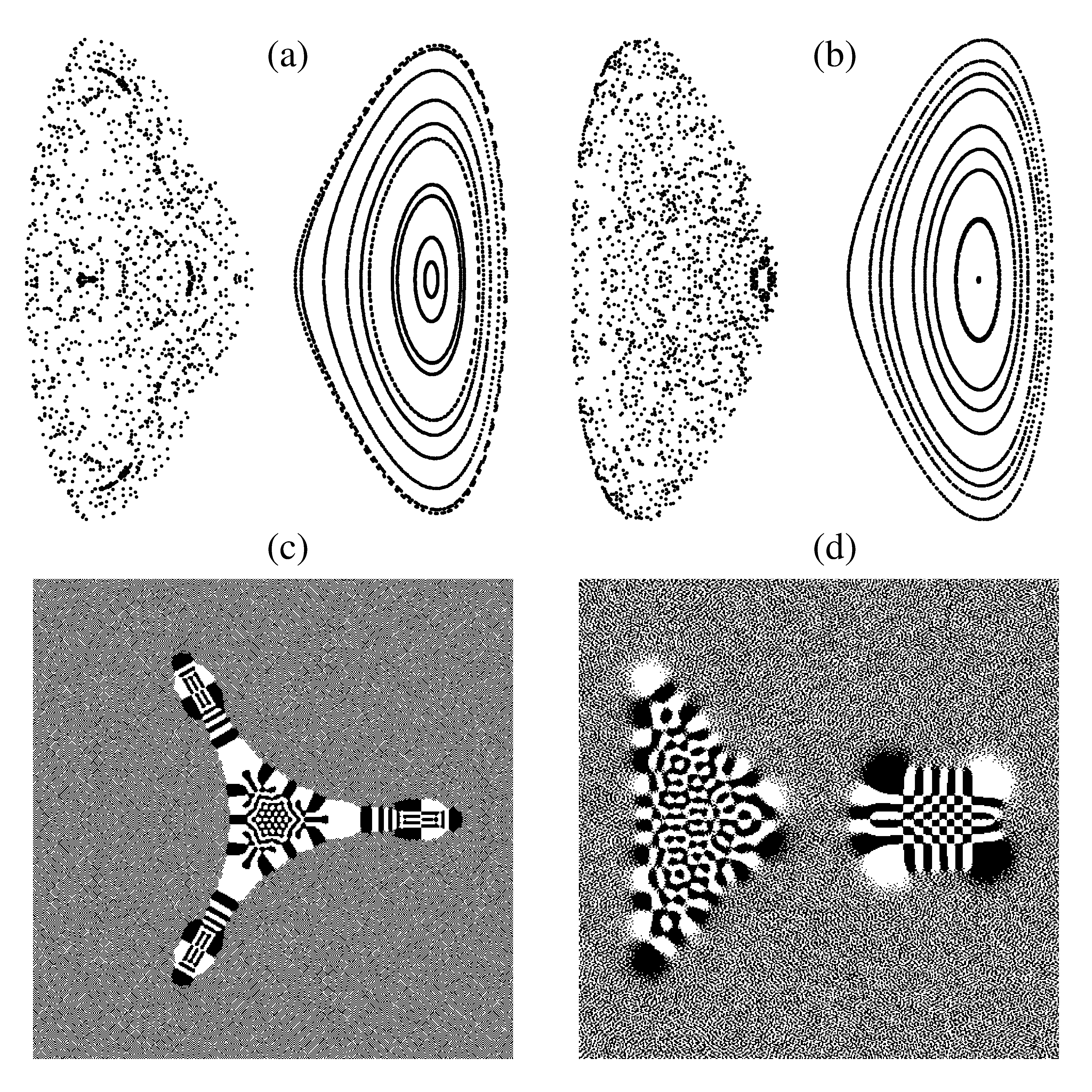
Figure 7.5: QMCS in the wave functions structure for $QO$(a,c) and $D_{5}$(b,d) potentials.

Let us note an additional advantage in nodal structure investigations for QMCS search in the mixed state case. In generic multi-well potentials, stationary wave functions as a rule are strongly localized in one or a few local minima. The localization rate is conveniently characterized by the dimensionless variable (for example in the case of two-well potential $D_{5}$)

$$\eta_{n}=\frac{P_{n}^{R}-P_{n}^{C}}{P_{n}^{R}+P_{n}^{C}},$$

where

$$P_{n}^{R}=\int\limits_{x>0}|\psi_{n}|^{2}dxdy$$

$$P_{n}^{C}=\int\limits_{x<0}|\psi_{n}|^{2}dxdy$$

Evidently $\eta=1$ for regular and $\eta=-1$ for chaotic states. Proximity of $\eta$ to unity is characterized by the variable

$$\xi_{n}=-sign(\eta_{n})\log_{10}(1-|\eta_{n}|)$$

Therefore $\xi_{n}=1$ corresponds to a wave function for $90\%$ localized in the regular minimum, and $\xi_{n}=-1$ — for $90\%$ in the chaotic one. In the mixed state case, the amplitude of overwhelming majority of wave functions in different local minima differs by several orders of magnitude (fig.7.6), which makes difficulties for analysis of the probability density distribution, but those difficulties are however inessential for the analysis of wave functions nodal structure.

Figure 7.6: Localization of the wave functions in $D_{5}$ potential.

7.2 Evolution of shell structure in the process of $R-C-R$ transition

Introduction of the stochasticity concept in nuclear theory made it possible to take a fresh look at the old paradox: how one could reconcile the liquid drop — short mean free path — model of the nucleus with the independent particles — gas-like shell model. To solve this paradox it is sufficient to assume the following:

1. When the nucleonic motion inside the nucleus is integrable, we expect to see strong shell effects in nuclear structure, quite well reproducible, for example, by the model of independent particles in the potential well.

2. If in the nuclear dynamics a chaotic component is dominant, it is necessary to expect, that the droplet model or Thomas-Fermi approximation will appear more useful.

With such an approach, the elucidation of the mechanism of destruction of shell effects in the process of the $R-C$ transition plays the key role. More appropriately the problem can be formulated in the following way: how does the shell dissolve with deviations from integrability or, conversely, how do incipient shell effects emerge as the system first begins to feel its proximity to an integrable situation?

As has been mentioned above, the finite motion of integrable Hamiltonian system with $N$-degrees of freedom, in general, is conditionally periodic, and the phase trajectories lie on $N$-dimensional tori. In the action-angle variables $(I,\theta)$ the Hamiltonian is cyclic with respect to angle variables, $H=H_{0}(I)$. Poincaré called the main problem of dynamics the problem of the perturbation of conditionally periodic motion in the system defined by the Hamiltonian

$$H=H_{0}(I)+\varepsilon V(I,\theta)$$

where $\varepsilon$ is a small parameter. The essential step in the solution of this problem was the KAM theorem, asserting, that at turning on non-integrable perturbation, the majority of non-resonance tori, i.e. the tori for which

$$\sum\limits_{i=1}^{N}n_{i}\frac{\partial H_{0}}{\partial I_{i}}\neq 0$$

are conserved, distinguishing from the unperturbed cases only by small (to the extent of smallness of $\varepsilon$) deformation. As was noted before, at definite conditions the KAM formalism allows us to remove the terms depending on the angle out of the Hamiltonian, using the convergent sequence of canonical transformations. When it succeeds, we find that perturbed motion lies on rather deformed tori, so that trajectories, generated by perturbed Hamiltonian remain quasi-periodic. In other words, the KAM theorem reflects an important peculiarity of classical integrable systems: they conserve regular behavior even at rather strong non-integrable perturbation. In the problem of our interest, concerning the destruction of the shell structure of quantum spectrum, the KAM theorem also will be able to play an important role. Considering the residual nucleon-nucleon interaction as non-integrable addition to the self-consistent field, obtained, for example, in the Hartree-Fock approximation, we can try to connect the destruction of shell with the deviation from integrability. The existence of shell structure at rather strong residual interaction (or at large deformation) can be due to the rigidity of KAM tori, contributing to survival of regular behavior. Such an assumption seems rather natural, especially if we take into account that the procedure of quasi-classical quantization [72, 73] itself as well as KAM theorem are based on convergence of the same sequence of canonical transformations.

The aim of this section is to trace the evolution of the shell structure of $QO$ Hamiltonian. In numerical calculations of this section it will be more convenient to use non-scaled version of the $QO$ Hamiltonian (2.2) . The unperturbed Hamiltonian $H_{0}$ we will understand as the Hamiltonian of two-dimensional harmonic oscillator with equal frequencies:

$$H_{0}\equiv H(a=1,b=0,c=0).$$

Its degenerate equidistant spectrum is well known. At switching on perturbation, the degeneration disappears and the shell structure forms. The number of states, for example the states of $E$-type (the numerical results, represented below, are relative to the states of this type, while analogous results are observed for the states belonging to another irreducible representations of $C_{3v}$-group) for the given quantum number $N$ is equal to

$$N_{0}=\frac{1}{2}(N_{1}+Mod(N,2)),$$

where

$$N_{1}=\frac{1}{3}(2N+Mod(N,3)),$$

and $Mod(N,M)$ is the remainder of division of $N$ by $M$.

It is obvious, that eigenfunctions of exact Hamiltonian $QO$ are no longer the eigenfunctions of operators $\hat{N}$ and $\hat{L}$. Nevertheless, as numerical calculations show, one can use the quantum numbers $N$ and $L$ for the classification of wave functions even at rather large nonlinearity. The measure of nonlinearity, at which such classification (i.e. the existence of shell structure) remains reasonable, is connected with quasi-crossing of neighboring levels. Quasi-crossing we shall understand as the approach of levels up to the distances of order of numerical calculations error.

The dependence of energy spectra of $QO$ Hamiltonian on the parameter $b$ for the values $W=3.9$ and $W=13$ are represented in Fig.7.7. As can be seen from Fig.7.7a, for the PES with $W=13$ at the approach to the line of critical energy of the transition to chaos, defined according to the negative curvature criterion, the destruction of shell structure, which we understand as the beginning of multiple quasi-crossings, takes place. At the same time, for PES with $W=3.9$ on Fig.7.7b quasi-crossings are absent even at larger nonlinearity than for $W=13$.

Figure 7.7: a) Energy spectra for QO Hamiltonian (2.2) depending on values of parameter $b$ for region $C$ $W=13$. Points mark the quasi-crossings of levels. Bold solid line shows the dependence of classical critical energy $E_{cr}$ on parameter $b$. The dashed line shows the quasi-crossing region border. Arrow shows the point of quasi-crossing of levels with numbers $k=40$ and $k=41$. b) Energy spectra for QO Hamiltonian (2.2) depending on values of parameter $b$ for region $C$ $W=3.9$. There are no quasi-crossings of levels.

The destruction of shell structure can be traced for the wave functions, using the analogue of thermodynamic entropy $S_{k}$ [75, 76],

$$S_{k}=-\sum|C^{k}_{NLj}|^{2}\ln|C^{k}_{NLj}|^{2}$$

The character of changes of entropy in regions $R_{1}$ and $R_{2}$, corresponding to regular classical motion, correlates with the transition from shell to shell (see Fig.7.8). Two effects are observed in the region $C$ corresponding to chaotic classical motion. Firstly, quasi-periodical dependence of entropy on energy is violated, which testifies to the destruction of shell structure. Secondly, monotone growth of entropy is observed on average with going out on the plateau corresponding to the entropy of random sequence at the energies essentially exceeding the critical energy.

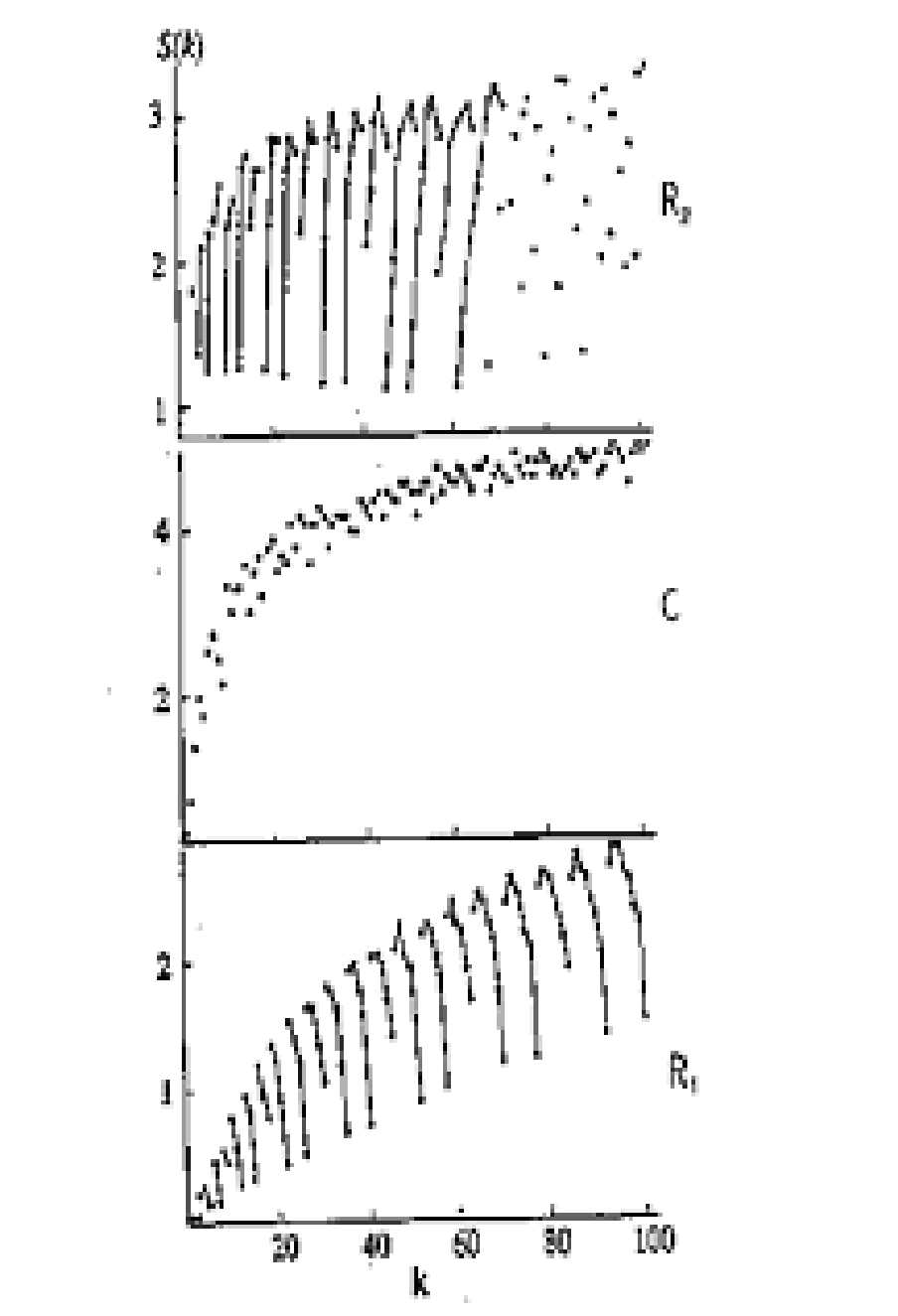
Figure 7.8: Entropy $S$ as function of the state number. The straight lines connect points corresponding to shell classification on the basis of $N$.

Chapter 8 Wave Packet Dynamics

The investigation of the time evolution of non-stationary states, i.e. of wave packets in quantum systems with classical analogues that admit chaotic behavior, provides important information about QMCS. The localized quantum wave packet (QWP) is the closest analogue of the point in phase space, which describes the state of a classical system. However, such correspondence between localized QWP and the classical point particle in the chaotic region is broken down for a very short time interval. Let us explain this fact by using Takahashi arguments [74]. We take two localized QWP $\Psi_{1}(\mathbf{x})$ and $\Psi_{2}(\mathbf{x})$ which are put in the chaotic region at an initial time to be slightly different from each other so that the difference between $\langle\Psi_{1}|\mathbf{\hat{x}}|\Psi_{1}\rangle$ and $\langle\Psi_{2}|\mathbf{\hat{x}}|\Psi_{2}\rangle$ (or $\langle\Psi_{1}|\mathbf{\hat{p}}|\Psi_{1}\rangle$ and $\langle\Psi_{2}|\mathbf{\hat{p}}|\Psi_{2}\rangle$) is very small. We assume that in chaotic region the localized QWP does not either extend in a certain time interval of the order $1/\sqrt{\hbar}$ like that in regular region. Hence, following the Ehrenfest theorem, the packets $\Psi_{1}(\mathbf{x})$ and $\Psi_{2}(\mathbf{x})$ move as classical particles and the distance between $\langle\Psi_{1}|\mathbf{\hat{x}}|\Psi_{1}\rangle$ and $\langle\Psi_{2}|\mathbf{\hat{x}}|\Psi_{2}\rangle$ (or $\langle\Psi_{1}|\mathbf{\hat{p}}|\Psi_{1}\rangle$ and $\langle\Psi_{2}|\mathbf{\hat{p}}|\Psi_{2}\rangle$) is increasing exponentially in time. Let us consider the superposition

$$\Psi(\mathbf{x})=\Psi_{1}(\mathbf{x})+\Psi_{2}(\mathbf{x}),$$ (8.1)

which also becomes a localized QWP in the initial state. From that assumption, we can expect that the QWP (8.1) does not extend in a certain time interval of the order $1/\sqrt{\hbar}$ . However, considering the exponential increment of the distance between $\langle\Psi_{1}|\mathbf{\hat{x}}|\Psi_{1}\rangle$ and $\langle\Psi_{2}|\mathbf{\hat{x}}|\Psi_{2}\rangle$, $\Psi(\mathbf{x})$ (8.1) extends exponentially in the chaotic region and does not behave as a classical particle. This result is inconsistent with initial assumption and implies that in the chaotic region localized QWP s (i.e. $\Psi_{1}(\mathbf{x})$, $\Psi_{2}(\mathbf{x})$ and $\Psi(\mathbf{x})$) extend exponentially as does the classical probability distribution in the first stage of time development.

In order to describe such unusual behavior of QWP we should address to the concept of quantum-mechanical phase space. There are a few well-established schemes to introduce phase-space variables in quantum mechanics. In the present study we shall follow the procedure proposed by Weissman and Jortner [77]. Let us consider an initially localized QWP $\Psi$ characterized by coordinates $\mathbf{q}$ and momentum $\mathbf{p}$,

$$\mathbf{q}=\langle\Psi|\mathbf{\hat{q}}|\Psi\rangle,\ \mathbf{p}=\langle\Psi|\mathbf{\hat{p}}|\Psi\rangle.$$

Now we introduce the coherent states $|\mathbf{p},\mathbf{q}\rangle$, which in the coordinate $x$-representation are given by Gaussian wave packets

$$\langle\mathbf{x}|\mathbf{p},\mathbf{q}\rangle=\prod\limits_{j=1}^{N}\left(\pi\sigma_{j}^{2}\right)^{\frac{1}{4}}e^{-\frac{(x_{j}-q_{j})^{2}}{2\sigma_{j}^{2}}+\frac{ip_{j}}{\hbar}\left(x_{j}-\frac{q_{j}}{2}\right)}.$$ (8.2)

In the study of a system of $N$ coupled harmonic oscillators, it is convenient to choose for constants $\sigma_{j}$ the rms zero-point displacements

$$\sigma_{j}=\sqrt{\frac{\hbar}{m_{j}\omega_{j}}}$$

where $m_{j}$ are masses and $\omega_{j}$ are frequencies of the uncoupled oscillators. With this choice of $\sigma_{j}$, the coherent states $\alpha\equiv|\mathbf{p},\mathbf{q}\rangle$ become the eigenstates of the harmonic oscillator annihilation operators

$$a_{j}|\alpha\rangle=\alpha_{j}|\alpha\rangle=$$ (8.3)

where

$$\alpha_{j}=\frac{1}{\sqrt{2}}\left(\frac{q_{j}}{\sigma_{j}}+i\frac{\sigma_{j}}{\hbar}p_{j}\right)$$

is a complex number.

Using these coherent states, it is possible to introduce the following quantum-mechanical phase-space density

$$\rho_{\Psi}(\mathbf{q},\mathbf{p})=|\langle\alpha|\Psi\rangle|^{2},$$

where $\Psi$ is any general wave packet. This quantum-mechanical coherent-state phase-space density may be regarded as a quantum analogue of classical phase-space density, since it satisfies an equation of motion where the leading term (when expanded in powers of $\hbar$), corresponds to the classical Liuville equation. The stationary phase space densities are the following

$$\rho_{E}(\mathbf{q},\mathbf{p})=|\langle\alpha|E\rangle|^{2},$$ (8.4)

where $|\alpha\rangle$ is given in terms of Gaussian wave packet (8.2), while the eigenstate $|E\rangle$ is given by squares of the projections of the eigenstates on the coherent state, Eq.(8.3). Using the well-known expressions for scalar products $\langle\alpha|NL\rangle$ we finally obtain

$$\rho_{E}(\mathbf{q},\mathbf{p})=\frac{1}{2}e^{-\frac{1}{2}(|\alpha_{+}|^{2}+|\alpha_{-}|^{2})}\sum\limits_{N,L}\frac{C_{NL}}{\sqrt{n_{+}!n_{-}!}}(\alpha_{+}^{*n_{+}}\alpha_{-}^{*n_{-}}+j\alpha_{+}^{*n_{-}}\alpha_{-}^{*n_{+}}),$$

where

$$\alpha_{\pm}=\frac{1}{\sqrt{2}}(\alpha_{2}\mp i\alpha_{1})$$

with

$$\alpha_{1,2}=\frac{1}{\sqrt{2}}(q_{1,2}+ip_{1,2}),\ n_{+}=\frac{N+L}{2},\ n_{-}=\frac{N-L}{2},\ j=\pm 1.$$

The phase-space density $\rho_{E}(\mathbf{q},\mathbf{p})$ is a function of the four real variables $p_{1},q_{1}$ and $p_{2},q_{2}$. We can get the contour maps of $\rho_{E}(p_{1},q_{1};p_{2},q_{2})$ in the $(p_{2},q_{2})$ plane, taking $q_{1}=0$ and calculating $p_{1}$ from the relation

$$H(p_{1},q_{1}=0,p_{2},q_{2})=E$$

Quantum Poincaré maps (QPM), obtained this way, constitute the quantum analogues of the classical Poincaré maps and can be used for the search for QMCS both in the structure of wave functions of stationary states and in the dynamics of wave packets.

Let us consider next the time evolution of a wave packet, which is initially in coherent state

$$|\Psi(t=0)\rangle=|\alpha\rangle$$

The time evolution of such initially coherent wave packet is given by

$$|\Psi(t)\rangle=\sum\limits_{k}|E_{k}\rangle\langle E_{k}|\alpha\rangle e^{-iE_{k}t}$$

The probability $p(t)$ of finding the system in its initial state — the survival probability — is given by

$$p(t)=|g_{\alpha}(t)|^{2}$$ (8.5)

where $g_{\alpha}(t)$ is the overlap of $\Psi(t)$ with the initial state

$$g_{\alpha}(t)=\langle\alpha|\Psi(t)\rangle=\sum\limits_{k}|\langle E_{k}|\alpha\rangle|^{2}e^{-iE_{k}t}.$$

Using the definition of stationary phase-space density (8.4), we can write

$$g_{\alpha}(t)=\sum\limits_{k}\rho_{E_{k}}e^{-iE_{k}t}.$$ (8.6)

Equation (8.6) implies that dynamics can be specified by the spectrum of the initial coherent state $|\alpha\rangle$.

Weissman and Jortner [77] have observed for Hénon-Heiles Hamiltonian two limiting types of QWP dynamics of initially coherent Gaussian wave packets, which correspond to quasiperiodic time evolution and to rapid decay of the initial state population probability. Quasiperiodic time evolution is exhibited by wave packets initially located in a regular region, while rapid decay of the initial state population probability is revealed by those ones that are initially placed in irregular regions. An analogous situation takes place also in the multi-well potentials of our primary interest, in the energy region where the mixed state is realized. The quantum correlator $p(t)$ for two-well potential $D_{5}$ reproduces well the characteristic properties of classical trajectories (see Fig.8.1): quasi-periodic motion in the regular minimum manifests itself in oscillations of the correlator, and chaotic motion in another local minimum — in fast decay of correlations.

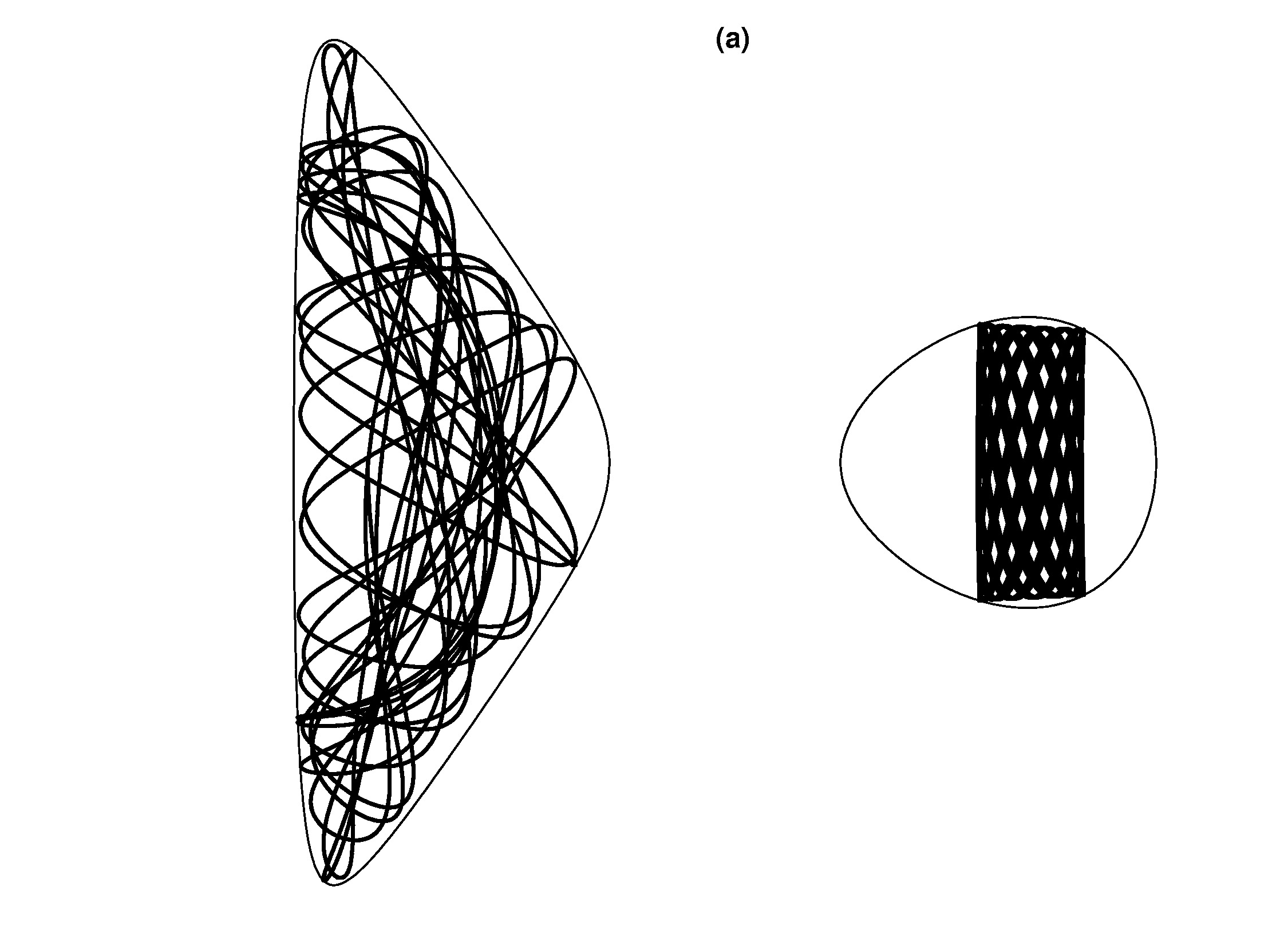
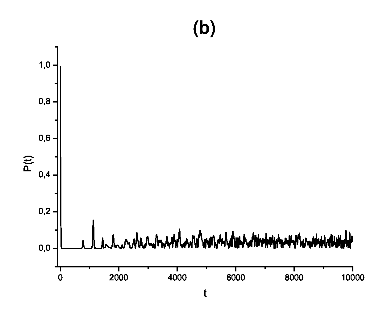
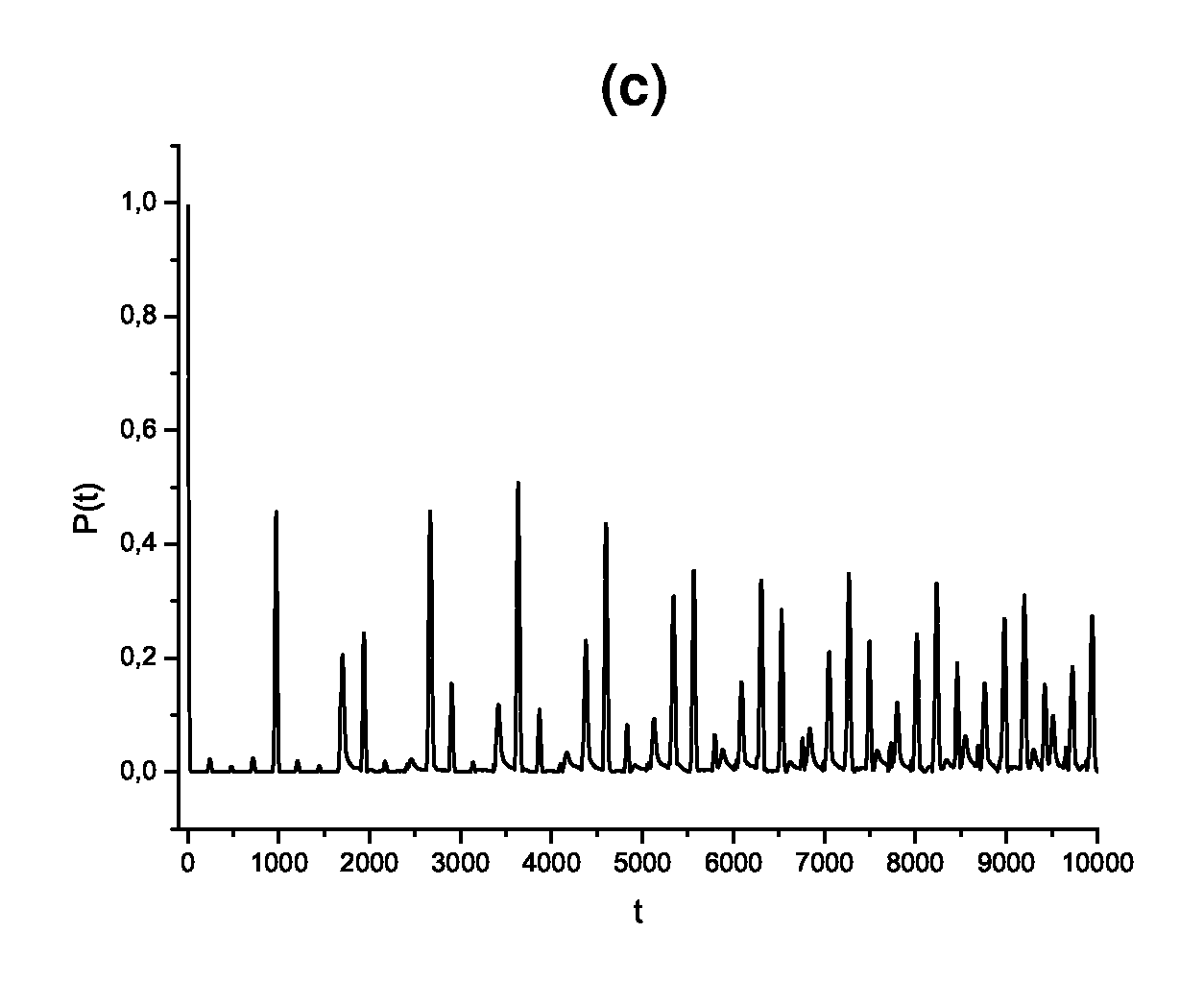
Figure 8.1: Typical trajectories for energies corresponding to the mixed state (a) and correlation functions (8.5) for equivalent Gaussian wave packets in chaotic (b) and regular (c) local minima of potential $D_{5}$ (2.4).

Let us turn to the consideration of the dynamics of QWP in the PES with a few local minima (QO with $W>16$) [27]. Transitions between different local minima can be divided into induced (the excitation energy exceeds the value of potential barrier) and tunnel transitions. The latter are subdivided into transitions from discrete spectrum into continuous spectrum (for example, $\alpha$-decay, spontaneous division), and from discrete spectrum into discrete spectrum (for example, transitions between isomeric states). Up to now the process of tunneling across a multidimensional potential barrier, when initial and final states are in discrete spectrum, has been the most complicated problem.

Most often the time evolution of wave packet is studied by two methods: either by direct numerical integration of the Schrödinger time-dependent equation with corresponding initial condition $\Psi(\mathbf{r},t=0)$, or by expansion of the packet $\Psi(\mathbf{r},t)$ in the eigenfunctions of the stationary problem. The first one has some shortcomings, e.g., the complication relative to the interpretation of the obtained results and the necessity of separating the contributions from sub-barrier and tunnel transitions for the packet of an arbitrary shape. These difficulties can be avoided if the sub-barrier part of the spectrum $E_{n}<U_{0}$ ($U_{0}$ is the height of the barrier) and the corresponding stationary wave functions $\psi_{n}(\mathbf{r})$ are known. Pure tunnel dynamics will take place for the packets representable in the form

$$\Psi(\mathbf{r},t)=\sum\limits_{n}C_{n}e^{-\frac{i}{\hbar}E_{n}t}\psi_{n}(\mathbf{r}),\ E_{n}<U_{0},$$

$$C_{n}=\int\Psi(\mathbf{r},t=0)\psi_{n}(\mathbf{r})d\mathbf{r}.$$

The probability $p^{R}(t)$ of finding the particle at the moment of time $t$ in certain local minimum $R$ is

$$p^{R}(t)=\int\limits_{R}|\Psi(\mathbf{r},t)|^{2}d\mathbf{r}=\sum\limits_{m,n}C_{m}^{*}C_{n}e^{\frac{i(E_{m}-E_{n})t}{\hbar}}\int\psi_{m}^{*}(\mathbf{r})\psi_{n}(\mathbf{r})d\mathbf{r}$$

or in the two level approximation

$$p^{R}(t)=p^{R}(0)-4C_{1}C_{2}\sin^{2}\left(\frac{i(E_{m}-E_{n})t}{2\hbar}\right)\int\psi_{1}^{*}(\mathbf{r})\psi_{2}(\mathbf{r})d\mathbf{r}.$$

Let us introduce the value

$$\bar{p}^{R}=\max_{\forall t}p^{R}(t)$$

which is the maximum probability of finding the particle in certain local minimum $R$, if initially it was localized to an arbitrary minimum. If the number of local minima is more than two, then of separateinterest is

$$\bar{\bar{p}}^{R_{0}}=\min_{\forall t}p^{R_{0}}(t)$$

i.e., the minimum probability to find the wave packet in the minimum $R_{0}$ corresponding to its initial localization.

Intuitively, we may suggest that $\bar{p}^{R}\approx 1$ if the initial minimum is local, and the final one is absolute. However, the results of [79] obtained for the simplest one-dimensional models (asymmetric double wells of different shapes) are inconsistent with the intuitive expectations. The probability of tunneling from the local minimum to the absolute one depends resonantly on the potential parameters. Fig.8.2 gives the dependence of $\bar{p}^{R}$ on the well depth displacement $d$. It can be seen that at an arbitrary asymmetry $\bar{p}^{R}\ll 1$.

Figure 8.2: Dependence of sub-barrier energy levels $E_{i}$ for a double asymmetric one-dimensional rectangular well with infinite external walls (above) and $\bar{p}^{R}$ on $d$ (below). Width of the well equals 3, width of the barrier — 1, barrier height — 2.

The resonant behavior of $\bar{p}^{R}$ becomes more clear if one considers the spatial structure of the sub-barrier wave functions. For a sufficiently wide barrier in the case of an arbitrary asymmetry, the sub-barrier wave functions are largely localized in separate minima. The delocalization takes place only in the vicinity of the level quasi-crossing. The degree of this delocalization directly depends on the distance between the interacting levels. Obviously, the QWP, in which the components localized in the certain minimum are dominating, cannot tunnel effectively to the neighboring minimum. It is precisely this reason that explains the stringent correlation between the $\bar{p}^{R}$ minima and the level quasi-crossing (see Fig.8.2).

Now the question arises if a similar correlation between the level quasi-crossings, the delocalization of wave functions and resonant tunneling persists in the two-dimensional case. To give an answer to this question let us turn to $QO$ Hamiltonian (2.2) in the region $W>16$. Recall that three ($C_{3v}$-symmetric) identical additional minima appear at $W>16$ apart from the central minimum. The central minimum exceeds the lateral ones in depth in the region $16<W<18$. At $W>18$, the central minimum becomes the local one. In this region of parameters the procedure of diagonalization of $QO$ Hamiltonian in oscillator basis becomes essentially complicated. It is connected with the fact that the basis of Hamiltonian, the potential of which has the unique minimum, is used for the diagonalization of Hamiltonian with complex topology of the PES. In addition to the large dimension of the basis, it is necessary for the basis wave functions to have sufficient value in the region of lateral minima. It has been achieved by the optimization of frequency $\omega_{0}$ of the oscillator basis. For the values of parameters used in the calculations ($W=17.8,\ b=0.17$) the value of the optimal oscillator frequency was $\omega_{0}=0.2$. Fig.8.3 gives lower eigenvalues of $E$ and $A_{1}$ types depending on the basis dimension. We can see that it is possible to get saturation in the basis at the dimension of sub-matrices $N\sim 10^{3}$ even for low states localized in the lateral minima (dashed lines).

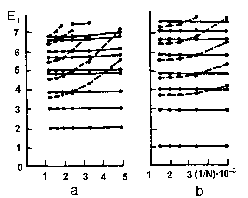
Figure 8.3: Dependence of the energy spectrum of $E$-type (a) at $b=0.173798$ and $A_{1}$-type (b) at $b=0.17$ on the dimension of sub-matrices $N$ for $W=17.8$. Dashed lines correspond to the states localized in peripheral minima.

We can also use the above introduced analog of thermodynamic entropy $S_{k}$ to estimate the degree of saturation in the basis. Fig.8.4 gives $S_{k}$ values for the states of $A_{1}$ type for the dimension of sub-matrices $408$ and $690$. Increasing of the basis dimension does not lead to significant changes of $S_{k}$ values for the states with energy up to the saddle one $E_{S}$.

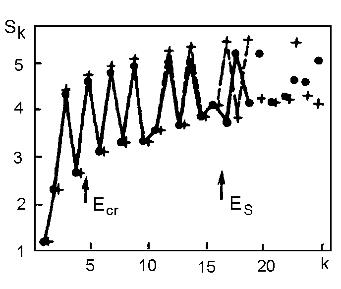
Figure 8.4: Dependence of $S_{k}$ on the state number $k$ ($A_{1}$-type) for the dimension of sub-matrices $408$ (dark points) and $690$ (crosses) at $W=17.8$ and $b=0.17$. $E_{S}$ corresponds to the saddle energy. and $E_{cr}$ — to the classical critical energy of the regularity-chaos transition.

The states localized in the central or in the lateral minima have essentially different distributivity of the coefficients $C_{i}^{k}$, $\{i\equiv NLj\}$ (see Fig.8.5a,b) and thus different entropies: states localized in the central minimum have less entropy. In the neighborhood of the points of level quasi-crossings, delocalization of wave functions corresponding to these levels takes place; these wave functions have close distributivity of the coefficients $C_{i}^{k}$ (see Fig.8.5c,d).

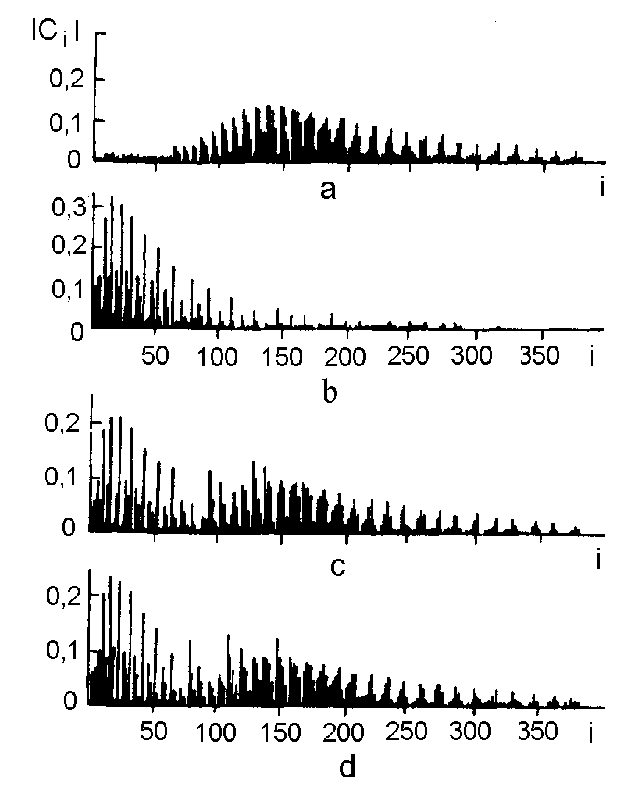
Figure 8.5: Distribution of coefficients $C_{i}^{k}$ by number of basis state $i=(NLj)$ ($E$ - type) for localized states with $k=3$ (a) and $k=4$ (b) at $b=0.17379$ ($W=17.8$) and for the delocalized states with $k=3$ (c) and $k=4$ (d) in the point of quasi-crossing $b=0.1737924$ ($W=17.8$).

Fig.8.6 shows the sub-barrier part of the energy spectrum obtained by the diagonalization. As is easy to see, the tunneling of the wave packet, composed of the sub-barrier wave functions, can be described in a two-level approximation. Indeed, there are approximately $10$ level quasi-crossings of $A_{1}$ and $E$-types, where the nonlinearity parameter $b$ changes are of the order of $10^{-2}$, while the effective half-width of the overlap integral in (3.66) is about $10^{-5}$ (see Fig.8.7). Hence, all non-diagonal elements will be close to zero with the overwhelming probability in the matrix

$$\alpha_{mn}=\int\limits_{R}\psi^{*}_{m}(\mathbf{r})\psi_{n}(\mathbf{r})d\mathbf{r}$$

of an arbitrary nonlinearity parameter (e.g., $b$). Two essential non-zero out-of-diagonal matrix elements (two-level approximation) appear only in the vicinity of quasi-crossings. The probability of double quasi-crossings at a fixed nonlinearity parameter is almost excluded. This probability is by two or three orders lower than that of rather rare $\sim 10^{-3}$ single quasi-crossings.

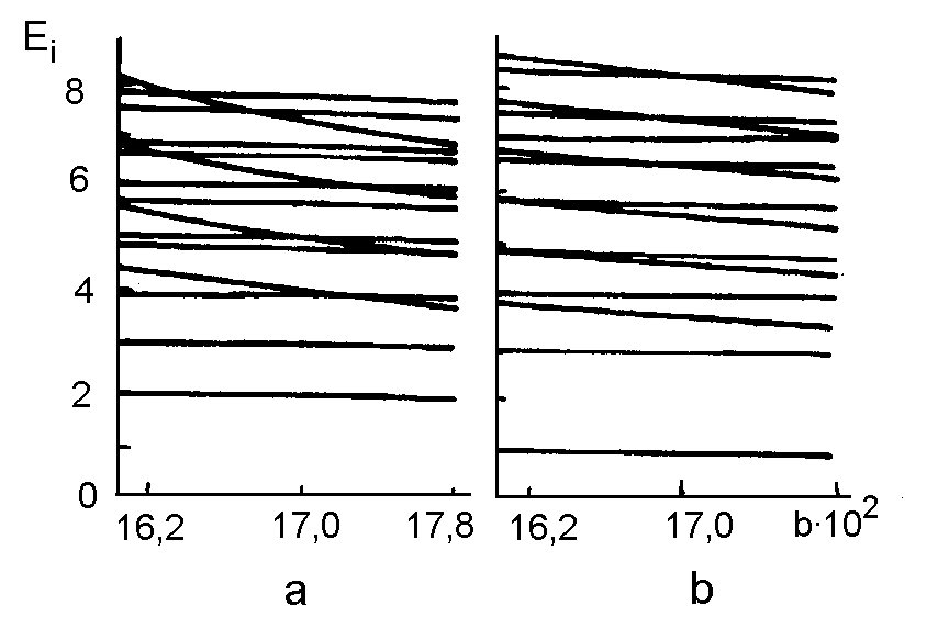
Figure 8.6: Dependence of energy levels $E_{i}$ of the $QO$ Hamiltonian (2.2) on the parameter $b$ for $W=17.8$: a) — spectrum of $E$-type, b) — spectrum of $A_{1}$-type.

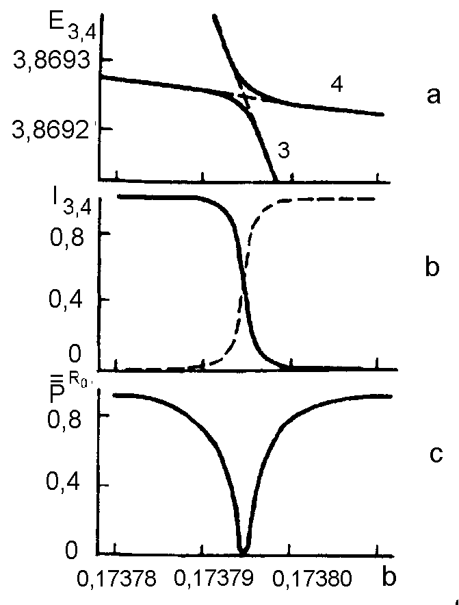
Figure 8.7: a) - Quasi-crossing of energy levels of $E$-type with $k=3,4$ for $QO$ Hamiltonian (2.2); b - localization of wave functions of states with $k=3,4$ in the central well at different $b$; c - dependence $\bar{p}^{R}(b)$.

So now we can give the answer to the question we have posed above. The stringiest correlations between level quasi-crossings, delocalization of wave functions and resonant tunneling across the potential barrier take place in the two-dimensional case (and, most likely, in the multi-dimensional one too).

The existence of the mixed state for many-well potentials must be clearly manifest in the dynamics of quantum wave packets. The pre-exponential factor of the tunnel amplitude depends on the type of classical motion and consequently we expect to observe asymmetry of the effective barrier penetration in the mixed state. This purely classical effect may be observed only if the uncertainty in level energy is comparable with the average distance between levels, and the system does not yet ”feels” that the spectrum is discrete. This determines the time scale for which observation of the effect is possible. It is the same time scale on which transition from classical diffusive evolution with linearly increasing energy to the quasi-periodical quantum one is observed [80].

8.1 Dynamical tunneling

Transition from integrability to chaos in classical dynamics not only significantly modifies the tunneling process, but moreover it leads to the appearance of principally new scenarios of the tunneling effect. The simplest example of such a scenario is the so-called dynamical tunneling [81]. Dynamical tunneling appears in systems where the phase space contains such regions that transition between them is forbidden in classical mechanics, but this restriction is not due to the potential barrier. Of course such an effect is possible in systems with two or more degrees of freedom, where additional to the energy integrals of motion are sources of the corresponding restrictions. This new type of tunneling is more complicated than the traditional (barrier) tunneling. The complication is connected with the fact that simple consideration of the potential energy surface does not reveal the conditions of the restriction. Instead of static potential surfaces one should consider dynamical behavior of the trajectories.

In order to understand the origin of dynamical tunneling in a bounded system, let us recall the semiclassical solution of the one-dimensional symmetric double well problem. If we quantize the system, considering each well separately, we obtain a spectrum composed from exactly degenerate doublets. Only by taking into account the interaction between the wells via overlap of exponentially small sub-barrier tails of the wave functions, we can obtain the correct result — almost degenerate pairs of levels with the well-known splitting. The magnitude of the latter determines the tunneling rate.

A situation similar to those in the one-dimensional symmetric double well can exist also in a multi-dimensional potential in the absence of energy barrier. Let us consider [82, 83, 84] a dynamical system with reflective symmetry of the phase space $T$. Let there be two non-connected regions $A_{1}$ and $A_{2}$ in the phase space, each of them being invariant with respect to classical dynamics, mapping one onto another with the symmetry transformation $A_{2}=TA_{1}$. Let the classical motion in $A_{1,2}$ be regular, i.e. those regions represent the stability islands embedded in the chaotic sea. In that case as we have seen above the regions $A_{1,2}$ represent invariant tori in classical phase space. We make an additional assumption that in the semiclassical limit there is a set of states $\psi(\mathbf{q})$ mostly localized in the regions $A_{1}$ and $A_{2}$. Using the standard procedure we can quantize motion in each region independently and construct degenerate wave functions $\psi^{(1)}(\mathbf{q})$ and $\psi^{(2)}(\mathbf{q})=\psi^{(1)}(T\mathbf{q})$, sometimes called quasi-modes. Taking into account the interaction between the regions, the quasi-modes $\psi^{(1,2)}(\mathbf{q})$, as in the one-dimensional case, must be replaced by their combinations — symmetric and antisymmetric:

$$\psi^{(\pm)}(\mathbf{q})=\frac{1}{\sqrt{2}}\left(\psi^{(1)}(\mathbf{q})\pm\psi^{(2)}(\mathbf{q})\right)$$

Energy degeneration between the functions is removed due to the tunneling processes. However, in contrast to the one-dimensional case, the invariant tori $A_{1,2}$ are not always separated by the energy barrier in the configuration space. Transitions $A_{1}\leftrightarrow A_{2}$ may be classically forbidden by conservation of the constant of motion distinct of the energy.

Like in the one-dimensional case, a wave packed constructed from linear combinations of the wave functions

$$\Psi^{(1,2)}(\mathbf{q})=\psi^{(+)}(\mathbf{q})\pm\psi^{(-)}(\mathbf{q})$$ (8.7)

will mimic a classical particle, initially localized in one of the regions $A_{1,2}$. The wave packet (8.7) will make the transitions between regions with the frequency determined by the energy splitting of states $\psi^{(+)}(\mathbf{q})$ and $\psi^{(-)}(\mathbf{q})$. A natural question arises: if in the phase of the system there are two symmetric stability islands separated by chaotic sea, then how that sea affects the dynamical tunneling between the islands? Semiclassical reasoning points out that the probability distribution associated with the wave function of the quantized torus decays exponentially outside the torus. The small overlap in the classically forbidden region of the decaying distributions, centered on the two congruent quantized tori, will lead to the tunneling splitting. If there is no chaotic region between the tori, then the overlap will be very small. However if a chaotic region exists between the tori, then the wave functions corresponding to the tori overlap initially with the chaotic states. Due to the ergodic nature of chaotic wave functions (uniform distribution of the probability density), the connection between the two tori appears to be more efficient that in the case of a regular intermediate state. Therefore we can expect that the tunneling will be assisted by the presence of the chaotic region.

All these qualitative considerations are confirmed by the analysis [82] of the splitting magnitude in the tunneling doublet as a function of the parameter $\sigma$ — the measure of chaoticity of the system. The splitting undergoes considerable fluctuations, which are connected with quasi-crossing of the ”outside” chaotic level and the considered regular tunneling doublet. It is important to note that because there is no dynamical fragmentation of the chaotic region on separated symmetric parts as happens in the regular part of the phase space, we have no reason to expect the appearance of chaotic doublets. So every chaotic state has fixed parity.

Peculiarities of such a spectral region can be described in the three-level model [83] defined by the Hamiltonian

$$\hat{H}=\left(\begin{array}[]{ccc}E+\varepsilon&0&0\\ 0&E-\varepsilon&\nu\\ 0&\nu&E^{C}\end{array}\right)$$ (8.8)

Here $E\pm\varepsilon$ are energies of the regular quasi-doublet, composed of the symmetric and antisymmetric combinations of the corresponding quasi-modes. The model assumes that the even chaotic state $|C\rangle$ with energy $E^{C}$ is connected with the $|+\rangle$ state with energy $E-\varepsilon$ by the coupling constant $\nu$. In practice one of the constants $\nu$ or $\varepsilon$ dominates. If $\varepsilon$ dominates then we turn back to the above considered two-level model. Therefore let us assume that the dominating constant is the coupling between the $|C\rangle$ and $|+\rangle$ states and let us take $\varepsilon=0$. In that case the doublet splitting $\Delta E$ will be governed by the energy shift $E_{+}$ due to the coupling $\nu$. Diagonalization of the Hamiltonian (8.8) leads to

$$\Delta E=\left\{\begin{array}[]{cc}\frac{\nu^{2}}{E-E^{C}}&E-E^{C}\gg\nu\\ |\nu|&E-E^{C}\ll\nu\end{array}\right.$$

It means that with the variation of $\sigma$ in the tunneling doublets splitting we will observe peaks with magnitude $|\nu|$ when $E^{C}(\sigma)$ crosses $E_{+}(\sigma)$.

Now we draw some conclusions. As distinct from the integrable case, systems with dynamics of mixed type, where the phase space contains both regular and chaotic regions, demonstrate a new tunneling mechanism called chaos assisted tunneling [82]. The doublets splitting that determines the tunneling rate in two-level approximation in systems of mixed type, is as a rule several orders of magnitude higher than for similar integrable systems. In contrast to direct processes when a particle tunnels directly from one state to another, chaos assisted tunneling corresponds to the following three-step process:

1. tunneling from a periodic orbit to the closest point in the chaotic sea;

2. classical propagation in the chaotic region of the phase space towards the vicinity of another periodic orbit;

3. tunneling from the chaotic sea onto the latter periodic orbit.

In other words doublet splitting due to reflective symmetry occurs not directly but through the compound-process of wave function destruction, piece by piece, near one regular region, and then chaotic transport through the chaotic sea towards the neighboring symmetry conjugated regular region, and at last restoration of the initial state image. Schematically this process is presented on Fig.8.9. Let us note that chaos assisted tunneling is a formally higher perturbative order process than direct tunneling. But the corresponding matrix elements for chaos assisted tunneling are much larger than for the direct process. Intuitively it can be pictured as the following: as the main part of the distance (through the chaotic sea) represents a classically allowed transition, then we can expect that those indirect trajectories will make a larger contribution to the tunneling flow than the direct ones. In the case of direct tunneling all sub-barrier trajectory represents a classically forbidden process.

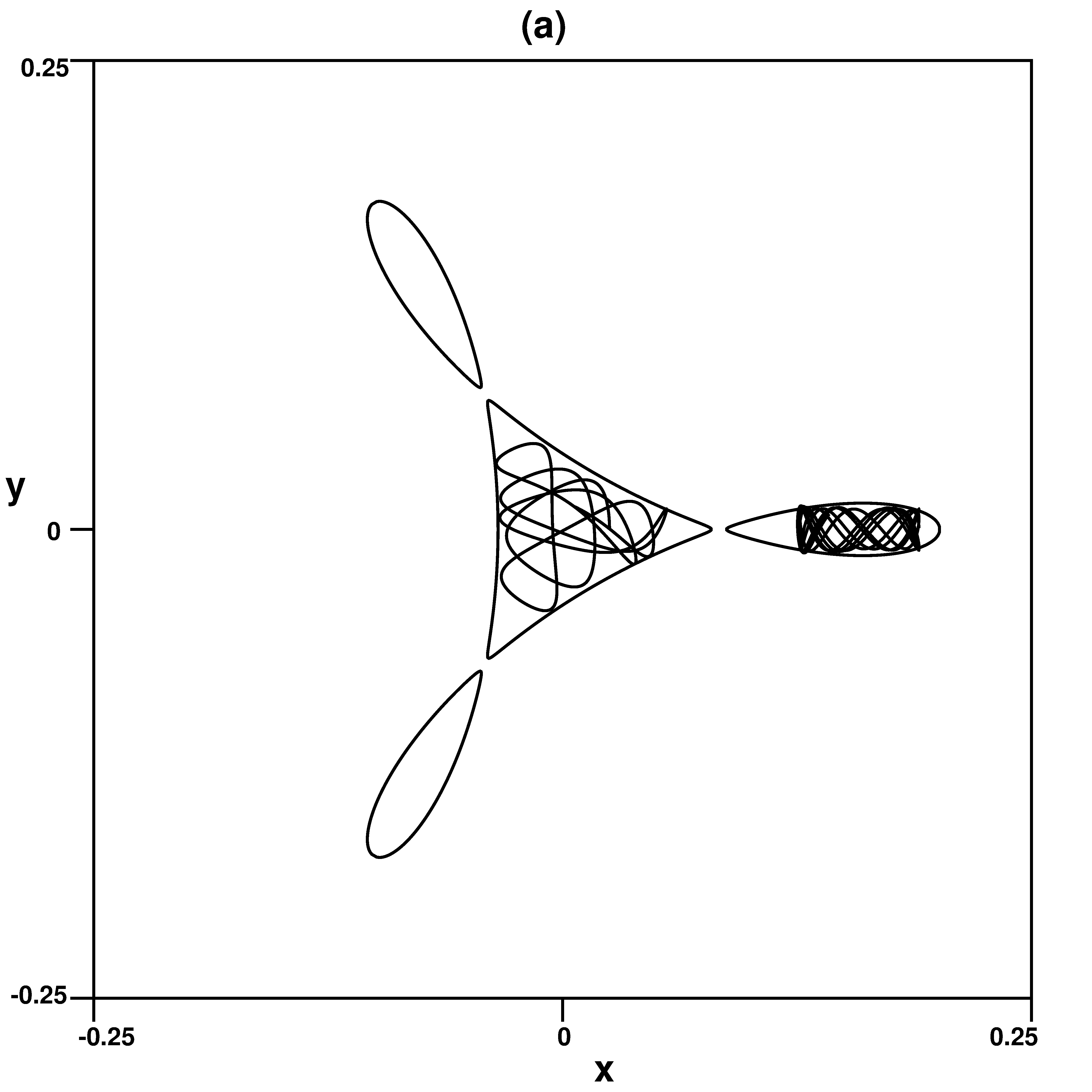
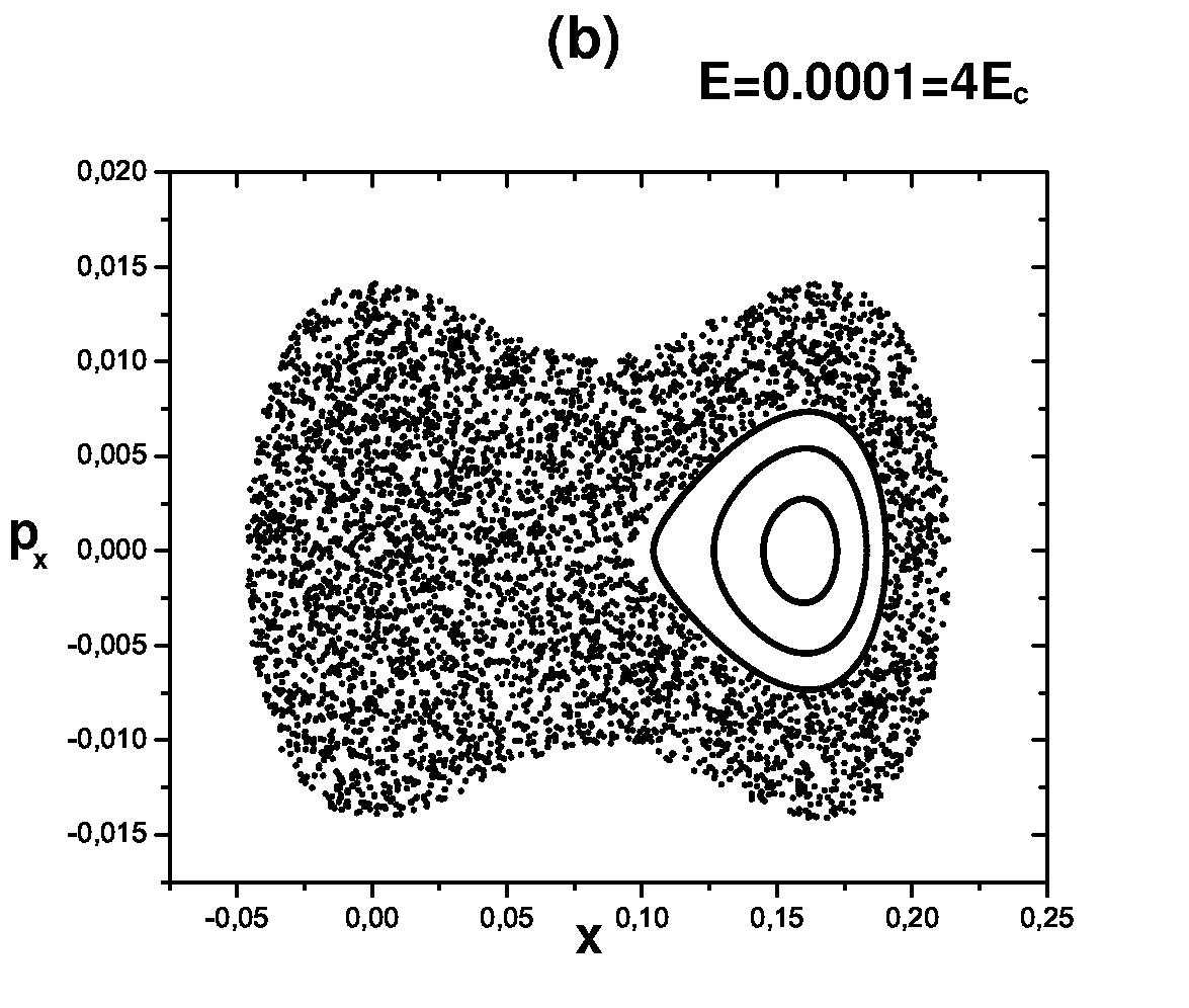
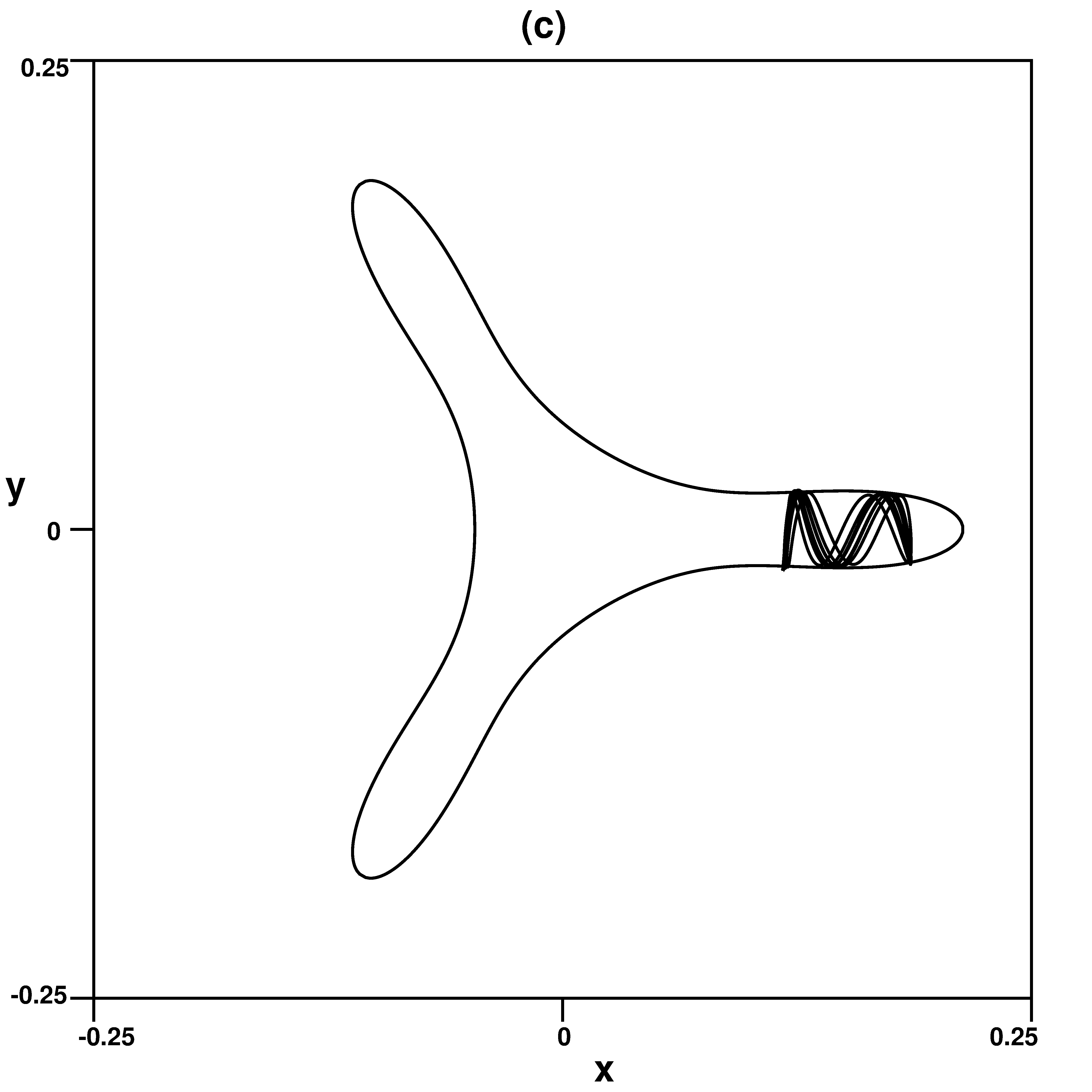
Figure 8.8: A schematic representation of direct and chaos assisted tunneling [85]

Figure 8.9: Regular and chaotic trajectories for $E\lesssim E_{S}$ (a), PSS (b) and regular quasiperiodic trajectory (c) for $E=2E_{S}$ in the $QO$ potential (2.3).

Let us now consider the dynamics of Gaussian wave packets in $QO$ potential (2.3) with $W=18$, when PES have four local minima — the central one with chaotic motion and three symmetric peripheral with regular motion for sub-barrier energies (see fig.8.9a).

At considerably super-barrier energies of motion, chaotic dynamics is observed in all local minima; however in the peripheral one, a large stability island survives even for $E=2E_{S}$ (fig.8.9b), which correspond to quasiperiodic trajectories localized in those minima (fig.8.9c).

With the spectral method it is easy to perform a numerical simulation of the dynamical tunneling process for super-barrier motion in $QO$ potential (2.3). In order to do that we prepare the initial state $\psi_{0}(x,y)$ in the form of a Gaussian minimum uncertainty wave packet (8.2) with such parameters $(x_{0},y_{0},p_{x0},p_{y0})$ that correspond to classical initial conditions for a trapped regular trajectory (fig.8.9c). For some time the quantum dynamics of such a wave packet will imitate classical motion on the semiclassical trajectory. After a sufficiently long period of time, the dynamical tunneling effect starts to be visible — the wave packet leaves the local minimum of its initial localization and appears in two others — a process forbidden in classical mechanics. After the same time period the wave packet more or less restores in its initial states (fig.8.12).

The oscillating nature of dynamical tunneling is clearly described in terms of the autocorrelation function (5.23) (fig.8.12 on the left). Its Fourier transform (fig.8.12 on the right) demonstrates three dominant states in the wave packet composition, that form the tunneling triplet (the right maximum on the $P(E)$ diagram is actually a very tiny tunneling doublet). Figure 8.12 shows the probability distribution $|\psi(x,y)|^{2}$ for all three members of the tunneling triplet in order of energy increasing: the intermediate state is purely regular and forms a tunneling doublet with the state of highest energy which is almost regular with a small admixture of chaotic modes. The lowest lying state is predominately chaotic and overlaps with only one of the tunneling doublet partners (the higher one). Repulsion of those states considerably broadens the level splitting in the tunneling doublet and therefore increases the tunneling rate substantially, which is the essence of the chaos assisted tunneling effect.

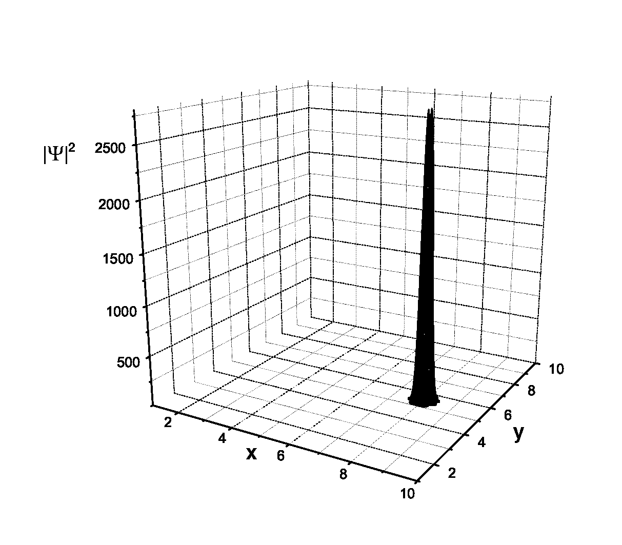
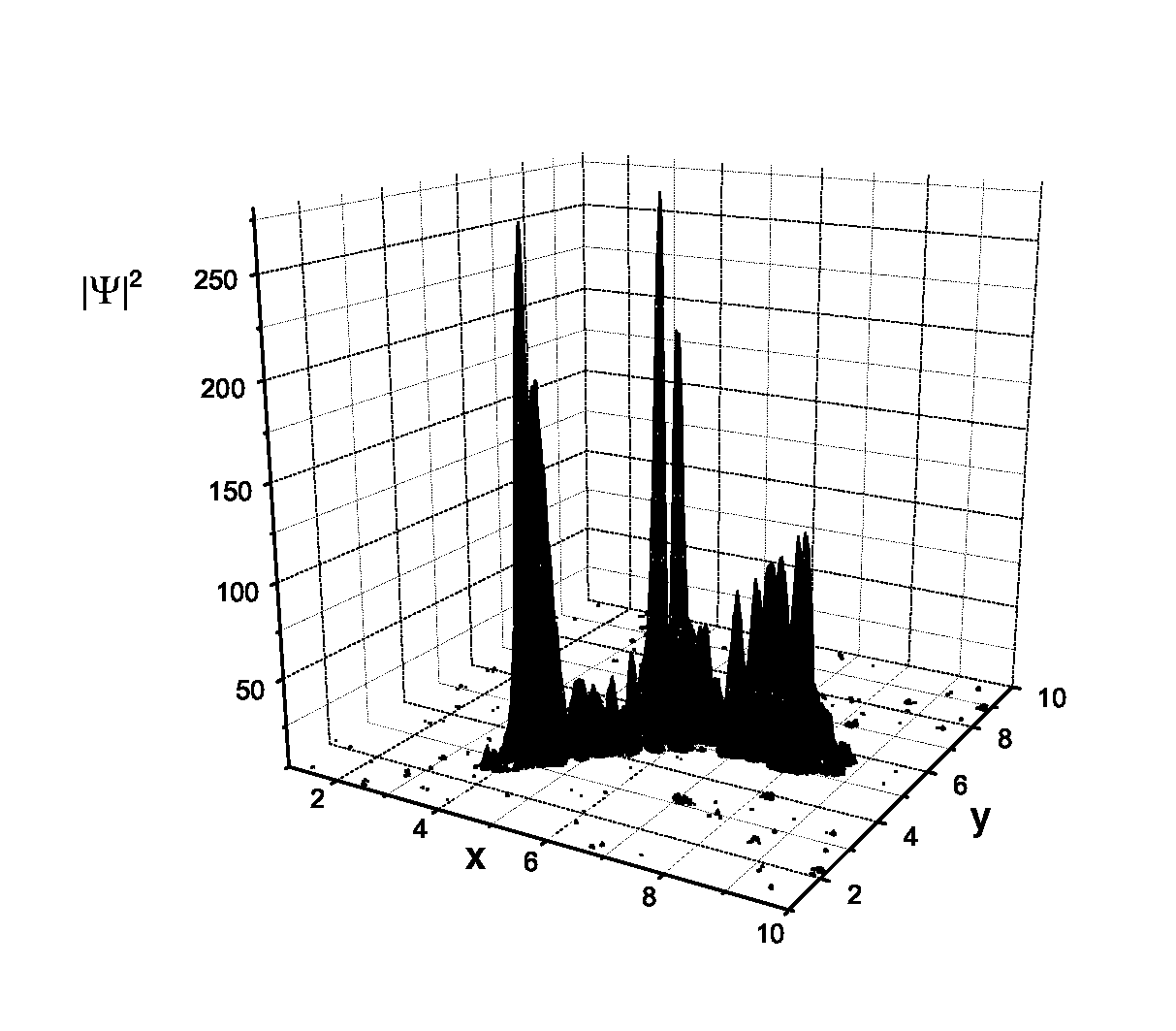
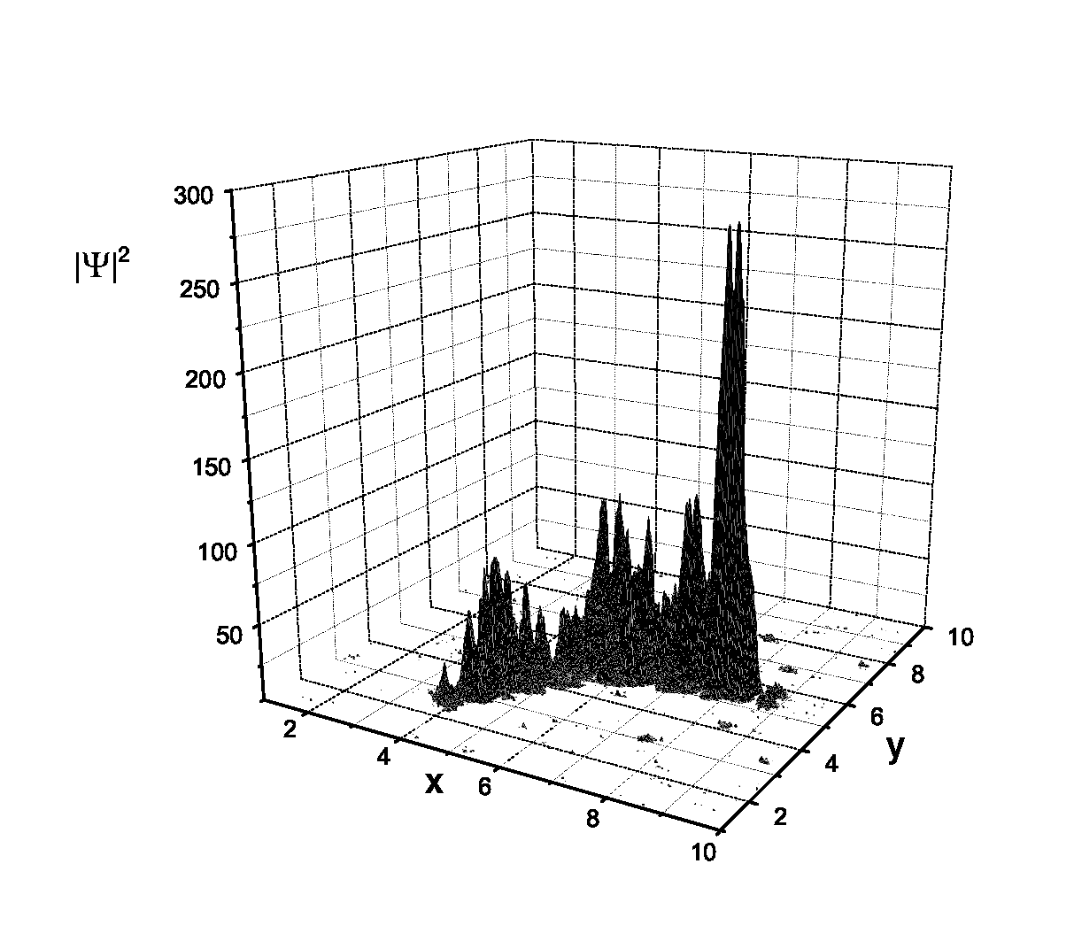
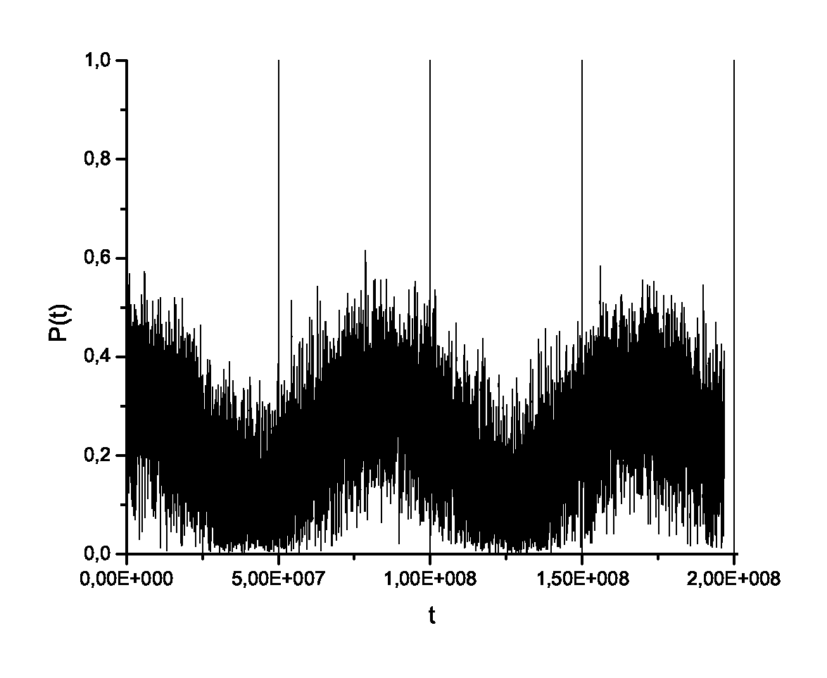
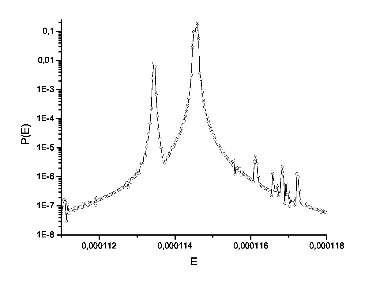
Figure 8.10: Temporal evolution of gaussian wave packet (8.2) under dynamical tunneling in the $QO$ potential (2.3).

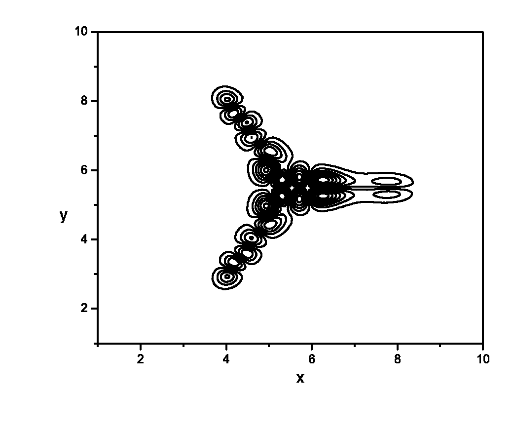
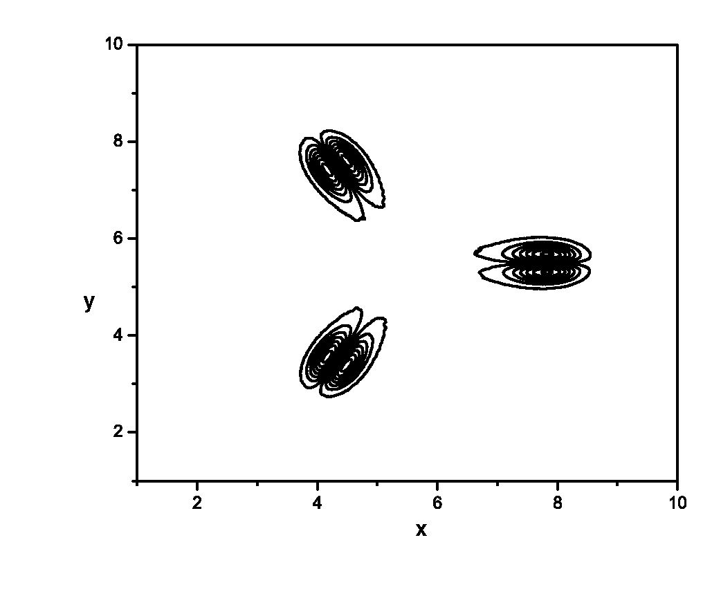
Figure 8.11: The auto correlation function (5.23) (left) and its Fourier transform (right) for Gaussian wave packet (8.2) tunneling dynamics in the $QO$ potential (2.3).

Figure 8.12: Level lines for $|\psi(x,y)|^{2}$ distribution for the tunneling triplet wave functions (the energy grows from left to right).

Chapter 9 The mixed state and concrete physical effects

9.1 Decay of mixed states

The escape of trajectories (particles) from localized regions of phase or configuration space has been an important topic in dynamics, because it describes the decay phenomena of metastable states in many branches of physics: chemical and nuclear reactions, atomic ionization, nuclear fusion and so on. This problem has a rich history. Almost a century ago, Sabine [86] considered the decay of sound in concert halls. Legrand and Sornette [87] have shown that this problem is equivalent to the escape one: a small opening of width $\Delta$ for escape must be identified with $\int\alpha(S)ds$, where $\alpha(s)$ is the absorption coefficient at position $S$ of the container (billiard) boundary, $\alpha(s)=1$ over the width of window and $\alpha(s)=0$ elsewhere. Szepfalusy and Tel [88] connected the escape problem with the problem of chaotic scattering.

Exponential decay is a common property expected in strongly chaotic classical systems [89, 90, 91]. Let us consider as an example [89] point particles in a rectangular box bouncing elastically off the walls. We allow our system to decay by providing a small window in one of the box walls through which particles are allowed to escape. As is well known, the motion of particle in a rectangular billiard is regular: two independent integrals of motion are the absolute values of momentum projection on the billiard walls. The trajectories of particles become chaotic if a circular scattering center is placed somewhere inside the box.

For the chaotic case, simple consideration leads to exponential decay. The number of particles leaving per time interval is given by

$$\frac{dN}{dt}=\Delta\rho(t)\int d^{2}p\ \mathbf{pe}_{n}=-2\Delta\rho(t)p^{2}\delta p$$ (9.1)

Here $p$ is the absolute value of momentum, $\mathbf{e}_{n}$ is a unit vector normal to the opening in the surface, and integration in momentum space is taken over a circular ring with radius $p$ and infinitesimal width $\delta p$. Function $\rho(t)$ is the phase space density, which in the ergodic motion is only a function of time. In our case

$$\rho(t)=\frac{N(t)}{2\pi p\delta pA_{c}}$$ (9.2)

where $A_{c}$ is total coordinate space area available. Inserting (9.2) into (9.1) yields

$$N(t)=N(0)e^{-\alpha t};\ \alpha=\frac{p\Delta}{\pi A_{c}}$$ (9.3)

Analytically calculated decay constant $\alpha$ is in a good agreement with the graphically extracted value.

Exponential law at extremely long times turns into the power law typical for decay of regular systems. One possible mechanism for generation of power tails is the effect of ”sticking” of the chaotic orbits to outer boundaries of stability islands [92], or a very similar effect connected with the existence of marginally stable periodic or ”bouncing ball orbits”. Although some qualitative models, which show how the algebraic tail emerges, were introduced in [93], no critical conditions for the distinct decay laws were formulated in terms of the billiard geometrical constrains. Experimental escape of cold atoms from a laser trap of billiard type with a hole was studied in [94, 95].

Transition from the billiard escape problem to escape from potential wells from one hand substantially broadens the number of possible applications, and on the other significantly complicates the problem. Of course, the one-well case is a simpler one. Zhao and Du [96] reported a study on the escape rates near the threshold of Henon-Heiles potential (3.3). Simulations performed by the authors show that the escape from a Henon-Heiles system at energy slightly exceeding the saddle one, follows an exponential law similar to chaotic billiard systems. They derived an analytic formula for the escape rate as a function of energy. The derivation is based on the fact that the phase space considered potential (as well as the billiards) is practically homogeneous near the saddle points. It should be noted that in such a case all trajectories with energy higher than the saddle one leave the potential well in finite time. The only problem to solve is to determine the probability of a particle to escape from the well in unit time interval.

We intend to study the particles escape from the local minima in the case when the phase space contains macroscopically significant components of regular as well as of chaotic type [97]. As we have seen, such a possibility is realized in potentials with several local minima in the form of a mixed state. The problem of particles escape from a potential well in the presence of the mixed state has an essential distinction from the one considered in [96]. Detailed analysis of the Poincaré sections for the potentials $D_{5}$ and $QO$, made in chapter 2, shows that in the ”regular” well at energy higher than the saddle, chaotic trajectories appear and their measure increases with energy growth. At the same time the regular trajectories remain mostly trapped in the well. The phase space of such a system contains macroscopic regions of both the regular and chaotic motion. Therefore the ensemble of particles initially situated in the well, divides on two components. So the ultimate problem is to determine the probability to escape per unit time for the chaotic component, and the relative measure of non-escaping trajectories trapped in the well.

Let us address again the example to above considered in details potentials of quadrupole oscillations (2.3) and umbilic catastrophe $D_{5}$ (2.4). In the first as well as in the second case, in some local minima up to the saddle energies the motion remains absolutely regular. Moreover, at energies significantly higher than the saddle energy (see fig.9.1) the phase space structure preserves division on chaotic and regular components. The latter is localized in the part of configuration space which corresponds to regular motion at energies below than saddle energies.

Figure 9.1: Poincaré surfaces of section $y=0$ in the $(x,p_{x})$ plane for the potentials $D_{5}$ (a) and $QO$ (b) for $E=2E_{S}$

This phase space structure leads to the fact that escape from such local minima has all the above mentioned properties of decay of chaotic systems, and also a diversity of principally new features, representing an interesting topic for conceptual understanding of chaotic dynamics, and for application as well. We are interested only in the ”first passage” effects, leaving aside the problem of dynamical equilibrium setup for the finite motion (for example, in $QO$ potential). It is important to stress that though we study the process of escape from a concrete local minimum, the over-barrier in the case of a mixed state has a specific memory: general phase space structure at super-saddle energies is determined by the characteristics of motion in all other local minima.

We carried out numerical simulation and analytical estimates [97] of trajectories escape in potentials $D_{5}$ and $QO$ through the hole over the saddle point. Results of the escape problem for systems with multi-component phase volume (regular and chaotic components) essentially depends on choice of initial ensembles for dynamical variables. Fig.9.2 presents the normalized particle number $N(t)/N(t=0)$ for $10^{6}$ initial conditions, uniformly distributed inside the right minimum in the potential $D_{5}\ (x>0)$, and peripheral minimum in the $QO$ potential $(x>1/12)$, together with the typical trajectories and Poincaré sections. The results for different potentials are evidently similar and have such characteristic features:

Figure 9.2: Decay law for mixed states in the $D_{5}$ (a) and $QO$ (b) potentials. Solid lines — numerical simulation for $E/E_{S}=1.1,1.5,2.0$; dotted and dashed lines — theoretically obtained exponential and linear decay laws respectively, zoomed on the inset figure in the lower left corners. Other inset figures represent the typical trajectories and Poincaré sections for the three different types of initial conditions: linearly escaping, exponentially escaping and non-escaping. Circles show the joining points between the linear and the exponential decay laws at critical time $t=\tau$.

• At times $t\rightarrow\infty$ decay law saturates at

  $$N(t\rightarrow\infty)=\rho^{(ne)}N_{0}$$

  where $\rho^{(ne)}$ is equal to the relative phase volume of ”never-escaping” trajectories, which represents the regular trajectories completely localized inside the considered minimum. All such trajectories, therefore, have infinite escaping times.

• For $t>\tau(E)$ the decay law has exponential form

  $$N(t)/N_{0}=\rho^{(ne)}+\rho^{(e)}e^{-\alpha^{(e)}(t-\tau)}$$ (9.4)

  where $\rho^{(e)}$ represents the relative number of exponentially escaping particles.

• $t<\tau(E)$ For the decay law is linear

  $$N(t)/N_{0}=1-\alpha^{(l)}t.$$ (9.5)

We should stress, that (9.5) is in no way a linear approximation of (9.4) for small $t$: in general $\rho^{(ne)}+\rho^{(e)}e^{-\alpha^{(e)}\tau}\neq 1$ and $\alpha^{(e)}\rho^{(e)}e^{-\alpha^{(e)}\tau}\neq\alpha^{(l)}$. Instead, from the condition of smooth joining of curves (9.5) and (9.4) in the transition point $t=\tau$, we obtain

$$\begin{array}[]{c}\alpha^{(e)}=\alpha^{(l)}/\rho^{(e)}\\ \rho^{(e)}=1-\rho^{(ne)}-\rho^{(l)}\end{array}$$

where $\rho^{(l)}=\alpha^{(l)}\tau$ is the relative number of linearly escaping particles. Moreover, already on time scales $t\lesssim\tau(E)$ linear decay law (9.5) is apparently different from its exponential analogue

$$N(t)/N(t=0)=\rho^{(ne)}+(1-\rho^{(ne)})e^{(-\alpha^{(l)}t)}$$

(see the inset on fig.9.2).

As we can see from the inset Poincaré section on fig.9.2 both the chaotic and regular trajectories contribute to linear escaping regime (9.5), because for sufficiently small times $t<\tau$ chaotic and regular motions are not yet distinguishable. Up to transient time $t=\tau$ all quasi-one-dimensional regular trajectories, oriented along the $x$-axis, have already escaped and for $t>\tau$ the escape of the remaining chaotic particles follows exponential law (9.4). The particles escaping the last show already mentioned sticking phenomena (see fig.9.2).

The transient time $\tau(E)$ in fact coincides with the passage time of the longest one-dimensional path from the opening to the opposite wall of the potential well and back (see fig.9.2). For the potentials $D_{5}$ and $QO$ corresponding theoretical estimates read (we assumed $m=1$)

$$\begin{array}[]{c}\tau_{D_{5}}(E)=2\int\limits_{0}^{\sqrt{2(1+\sqrt{E})}}\frac{dx}{|p|}=\frac{\sqrt{2}}{E^{\frac{1}{4}}}K\left(\sqrt{\frac{1+\frac{1}{\sqrt{E}}}{2}}\right)\\ \tau_{QO}(E)=12\left(\frac{E_{S}}{E}\right)^{\frac{1}{4}}K\left(\sqrt{\frac{1+\sqrt{\frac{E_{S}}{E}}}{2}}\right)=6\sqrt{2}\tau_{D_{5}}(\frac{E}{E_{S}})\end{array}$$

where $K(k)$ is the complete elliptic integral of the first kind and $E_{S}=1/12^{4}$ is the saddle energy in the $QO$ potential for $W=18$ (for the $D_{5}$ potential $E_{S}=1$).

Theoretical estimates for the escape rate were obtained by averaging the escape probability over the opening [96]:

$$\alpha(E)=\rho(E)\int\limits_{x=x_{S}}dy\int\limits_{-\frac{\pi}{2}}^{\frac{\pi}{2}}d\theta|p|\cos\theta,$$

where $x_{S}$ is the coordinate of saddle point and $\rho(E)$ is the normalized particle density:

$$\rho(E)=\frac{1}{2\pi A(E)},$$

where $A(E)$ denotes area of the classically allowed region inside the well:

$$A(E)=\int\limits_{x>x_{S}}dxdy\Theta\left(E-U(x,y)\right).$$

Such $\rho(E)$ corresponds to uniform distribution of particles on the energy surface $H(\mathbf{p,q})=E$.

For the potentials $D_{5}$ and $QO$ the explicit formulae are the following:

$$A_{D_{5}}(E)=2\int\limits_{0}^{\sqrt{2(1+\sqrt{E})}}dx\sqrt{\frac{E-\left(\frac{x^{2}}{2}-1\right)^{2}}{x+2a}}$$

$$A_{QO}(E)=\frac{1}{72}\int\limits_{0}^{\sqrt{1+\sqrt{\frac{E}{E_{S}}}}}d\xi\sqrt{(\xi+4)^{2}-7}\times$$

$$\times\sqrt{\sqrt{1+\frac{\frac{E}{E_{S}}-\left(\xi^{2}-1\right)^{2}}{[(\xi+4)^{2}-7]^{2}}}-1}$$

where $\xi=\sqrt[4]{E_{S}}(x-x_{S})$.

Finally, the general expression for the escape rate is

$$\alpha(E)=\frac{\langle p\rangle}{\pi A(E)}.$$

For our case $\langle p\rangle=\int\limits_{x=x_{S}}dy|p|$. In the case of billiards with small opening $p=const\Rightarrow\langle p\rangle=p\Delta$, and we recover expression (9.3). For the potentials $D_{5}$ and $QO$ we get the results in closed form:

$$\alpha_{D_{5}}(E)=\frac{E-1}{2\sqrt{a}A_{D_{5}}(E)}$$

$$\alpha_{QO}(E)=\frac{\sqrt[4]{\varepsilon}}{12\pi A_{QO}(E)}\left\{\left(16\sqrt{\varepsilon}+1\right)K\left(\sqrt{\frac{1-\frac{1}{16\sqrt{\varepsilon}}}{2}}\right)-2E\left(\sqrt{\frac{1-\frac{1}{16\sqrt{\varepsilon}}}{2}}\right)\right\}$$

where $\varepsilon=E-E_{S}+1/256$, $K(k)$ and $E(k)$ are the complete elliptic integral of the first and second kind respectively.

In order to obtain $\alpha^{(l)}(E)$ we correct $A(E)$ subtracting the relative phase space occupied by the non-escaping particles

$$A^{(l)}(E)=A(E)(1-\rho^{(ne)})\Rightarrow\alpha^{(l)}(E)=\frac{\alpha(E)}{1-\rho^{(ne)}}$$

Fig.9.2 demonstrates good agreement between our theoretical and numerical results for a wide energy range.

The fraction of the non-escaping particles $\rho^{(ne)}$ coincides with the relative phase space volume of trajectories, localized in the regular minimum, which may be well estimated by the relative area of the stability island $\rho^{(si)}$ on the Poincaré section (fig.9.2). Calculation of the relative area of regular island in the Poincaré section was performed by the following scheme. By numerical integration of equations of motion the island boundary was determined and then the interior area was calculated. Further the obtained area was divided on the entire area of classically allowed motion, defined by the conditions $x>0$ and $p^{2}>0$. While the phase volume itself is 4-dimensional, the stability island in Poincaré section is 2-dimensional, and so we cannot expect absolute coincidence of the corresponding measures. However, the calculations show very close correspondence between them (see fig.9.3). Therefore, numerical analysis of Poincaré sections together with our theoretical results gives all the information necessary to predict the escape dynamics by an independent method.

Figure 9.3: Correlations between relative area of the stability island $\rho^{(si)}(E)$ and non-escaping particles ratio $\rho^{(ne)}$: empty squares – $\rho^{(si)}_{D_{5}}(E)$, filled squares – $\rho^{(ne)}_{D_{5}}(E)$, empty circles – $\rho^{(si)}_{QO}(E)$, filled circles – $\rho^{(ne)}_{QO}(E)$.

In summary, we have considered classical escape from separated local minima in two representative $2D$ multi-well potentials, realizing the mixed state. We have found that escape from regular minima contains a number of new features. The most important among them are the following: i) decay law saturates at long time ranges; ii) on small time scales there exists a linear segment, which is not connected with linear approximation to the exponential decay law observed in chaotic systems with homogeneous phase space. The fraction of particles, remaining in the well is determined by the relative phase volume of the regular component, which in its turn monotonically decreases with growth of energy. It was shown that the linear segment of the decay law is generated by the quasi-one-dimensional trajectories, oriented perpendicular to the opening, and the transient time of the linear-to-exponential regime lies in perfect agreement with the analytical estimates.

We should note that we devote our main attention to escape from the regular local minima, because the specifics of the mixed state manifests only in them. However let us recall that in the case of mixed state the phase space structure at super-saddle energies is determined by dynamical characteristics in different local minima of the whole potential energy surface.

The above mentioned peculiarities of the escape problem may have found practical application for extraction of the required particle number from atomic traps. Changing the energy of particles trapped inside the regular minimum, we can extract from the trap any required number of particles. The problem of particle energy changing in the potential well may be solved by the introduction of small dissipation. The obtained results may be of interest also for the description of induced nuclear fission in the case of double-humped fission barrier. Revealed peculiarities must manifest also in over-barrier dynamics of wave packets, initially localized in the regular minima.

9.2 Chaos assisted tunneling in superdeformed nuclei

Since its discovery the atomic nucleus has been constantly used for verifying new physical ideas such as superfluids, superconductivity, supersymmetry and dynamical chaos. The aim of this section is to demonstrate the possibility of observing the above mentioned features of chaotic multi-well dynamics in concrete physical effect — the decay of the superdeformed states of atomic nuclei. In contrast to the classical decay of the mixed state considered above, this effect is purely quantum, but nevertheless dependent on the structure of the classical phase space.

The superdeformed (SD) nucleus has an ellipsoid shape with axes ratio $a/b\sim 2$. Such extreme nuclei shapes are the result of the quantum nature of particles that compose the nucleus and fill the discrete energy levels (shells). In large deformations, the energy interval (gap) between filled and next free shells could be very large. In combination with other effects this energy gap could provide stability of the nucleus in such large deformations. Superdeformed nuclei were found more than twenty years ago [98], and today they have been observed in several mass regions around $A=20,40,80,130,150,165,190$ and $240$ [99].

Study of SD nuclei offers a new way of understanding nuclear structure. This is a good illustration of the above mentioned fact that nuclei are a laboratory for research of the general physical effects such as tunneling, chaos and phase transitions. On the one hand, nuclei provide interesting data for the study of these general phenomena. On the other hand, we obtain new information about nuclear structure.

SD nuclei are produced in reactions with heavy ions. Initially accelerated heavy ions, when colliding with nuclei of target material, produce highly excited and fast rotating compound nuclei. These nuclei release part of the excitation energy by the emission of light particles (neutrons, protons, alpha particles) and photons. In all observations of fast rotating SD nuclei, rotation breaks off (already at low momentum), when nucleus suddenly changes shape and decays to the state that corresponds to lower deformations. Three stages of the transition from SD state to the normal deformed (ND) one are presented on the fig.9.4 [100]: feeding of superdeformed bands, ordered rotation and decay from superdeformed to normal states.

Figure 9.4: The three stages in the ”life” of a superdeformed nucleus together with some characteristic properties [100].

The lowest states in SD local minimum correspond to high excitations in the main minimum. As a result, the lowest SD states (cold states) are characterized by good quantum numbers and symmetries, while their decays to the main minimum are controlled by strict rules of selection. In contrast, ND states at the same energy could correspond to chaotic motion in the semi-classical limit. Statistical analysis confirms this idea: energy spectrum in the region $E_{ext}\sim 6-7Mev$ demonstrates all the signs of chaos, while yrast region is regular [101]. This means that in the considered region of nuclei excitation for which deformation potential allows for the existence of second minimum, there is realized a mixed state, considered in detail through the present report. In that case a natural question arises: can the chaos assisted tunneling mechanism be used for description of the transition from the SD state to the ND one? We should stress that we can consider dynamical tunneling because the transition takes place in multi-dimensional space: nuclear shape is characterized by at least two parameters.

Aberg [102] estimated chaos assisted tunneling in perturbation theory. In the limit of no mixing between the ND states (completely regular ND system) the wave function of the SD state mixes with the doorway state only. In this case the tunneling probability is given by

$$T^{regular}\approx\left(\frac{V_{t}}{\Delta E}\right)^{2}$$

where $V_{t}$ is tunneling coupling between SD and doorway states, and $2\Delta E$ is the energy distance between the doorway states.

In the other limit situation (quantum chaos) the tunneling strength is spread out over all ND states. Because tunneling probability in the chaotic case is

$$T^{chaotic}\approx\left(\frac{V_{t}}{\Delta E}\right)^{2}N.$$

Consequently

$$\frac{T^{chaotic}}{T^{regular}}\approx N\approx\frac{\rho_{ND}(E)}{\rho_{doorway}}$$

For $\rho_{doorway}\approx 1\ Mev^{-1}$, and relative excitation energy between the SD and ND state $E=3-5\ Mev$ $\rho_{ND}/\rho_{doorway}\approx 10^{4}-10^{6}$. Therefore we expect the tunneling probability to be enhanced by $10^{4}-10^{6}$ times if the ND states are chaotic. In other words, the tunneling process connected to the decay out of superdeformed states is strongly enhanced by chaotic properties of the ND states.

Chapter 10 Conclusions

Autonomous Hamiltonian systems with many local minima describe a variety of physical processes, including chemical nuclear reactions, nuclear fission, phase transitions etc. Nevertheless, the potentials of non-trivial topology still remain far aside of attention, from both the technical and ideological difficulties. The present work is one of the first studies of regular and chaotic classical and quantum dynamics in multi-well potentials.

The most general type of classical motion in potential with two and more local minima represents the so-called mixed state, which was first observed for simple polynomial 2D potentials. We proposed quantum mechanical treatment of the mixed state, and demonstrate signatures of quantum chaos in the energy levels statistical properties, stationary wave function structure and Gaussian wave packets dynamics. In particular, we have presented a new approach to the investigation of QMCS in wave function structure, which can be realized in potentials with two or more local minima. The main advantage of the proposed approach is the possibility to detect QMCS in comparison not different wave functions, but different parts of the same wave functions. Efficiency of the approach was demonstrated for the deformational potential of surface quadrupole oscillations of nuclei and lower umbilic catastrophe $D_{5}$.

In this work we study the energy spectra statistical properties in the case of the mixed state. Spectral series in the energy ranges, where the mixed state is realized, open new possibilities for studies of intermediate statistics. At these energies chaotic and regular components are separated not in phase space (as usually the case), but in the configuration space. A priori the nearest neighbors spacing distribution function in the mixed state does not obviously reduce to the properly weighted superposition of Poisson and Wigner distributions. In the mixed state we deal not with statistics of a mixture of two level systems with different nearest neighbors spacing distribution functions, but with statistics of a level system, where each level does not belong to definite statistics. Statistical properties of such systems still wait investigation, however such systems correspond to the common case situation.

The solution of Schrödinger equation for two-dimensional potential systems of general form imposes high requirements on efficiency of numerical methods used. The matrix diagonalization method is efficient for one-well potentials. However, this numerical procedure becomes less attractive at the transition to multi-well potentials. We have shown that, in this case an attractive alternative to the matrix diagonalization may become the spectral method. The advantages of the spectral method compared to the diagonalization method are demonstrated in the analysis of quantum chaos problems for two-dimensional potentials with complicated geometry.

The report presents also some concrete realizations of physical effects, connected with the mixed state. Having considered classical escape from 2D multi-well Hamiltonian system, realizing the mixed state, we show that escape from local minima has a diversity of principally new features, representing an interesting topic for conceptual understanding of chaotic dynamics and applications.

In conclusion, let us dwell on open problems. Configuration space for multi-well potentials breaks up naturally into different regions (separate local minima); in each of them different dynamical regimes are realized. Thus, there is a need for a calculating scheme that will enable us to use the partial information about each isolated region with the aim of obtaining a solution of the full problem. We believe that the path decomposition expansion of Auerbach and Kivelson [103] will prove to be useful for describing the mixed state. This formalism allows the expression of the full time evolution operator as a time convolution and surface integrations of products of restricted Green functions, each of which involves the sum over paths that are limited to different regions of configuration space. Even for complicated nonseparable potentials qualitative behavior is readily inferred and quantitative solutions can be obtained from knowledge of the classical dynamics.

In the late 1990s Zaslavsky and Edelman [104] considered a model of a billiard-type system, which consists of two chambers connected through a hole. One chamber has a circle-shaped scatterer inside, and the other one has a Cassini oval with a concave border. As was shown, the corresponding distribution function does not reach equilibrium even during an anomalous large time. We want to emphasize, that the mixed state, at energy a little exceeding the saddle one, can serve as a more realistic model for studies of anomalous kinetics.

Bibliography

- [1] Zaslavsky, G.M. (1985) Chaos in Dynamical Systems, N.Y.: Harwood.
- [2] Haake, F. (1991) Quantum Signatures of Chaos, Berlin: Springer.
- [3] Gutzwiller, M., (1991) Chaos in Classical and Quantum mechanics, Berlin: Springer.
- [4] Gutzwiller, M., (1982) Physica D183.
- [5] Reichl, L.E. (1992) The Transition to Chaos, Berlin: Springer.
- [6] Krylov, N.S., (1950) Works on foundation of statistical physics, Moskow: NAS of USSR.
- [7] Poincaré, H., (1892) Les Methods Nouvelles de la Mechanique Celeste, Paris: Gautheir-Villars.
- [8] Baranger, M., (1989), MTI preprint, CTP 1808.
- [9] Bolotin, Yu.L., Gonchar, V.YU., Inopin, E.V., (1987) Yad.Phys., 45, 350.
- [10] Eizenberg. J., Greiner, W., (1976) Microscopic Theory of the Nucleus, Amsterdam-London: North-Holland.
- [11] Mosel, V., Greiner, W., (1968), Z. Phys., 217, 256
- [12] Henon, M., Heiles, C., (1964), Astron. J., 69, 73
- [13] Seivert, M., Ramayya, A.V., Maruhn, J., (1984), Phys.Rev. C29, 284
- [14] Poston, T., Stewart, N.I., (1978) Catastrophe Theory and Application, London: Pitman
- [15] Chirikov, B.V.,(1959), Atom. Energy, 6, 630
- [16] Doviel, P., Escande, D., Codacconi, J., (1983) Phys. Rev. Lett., 49, 1879
- [17] Rechester, A., Stix, T., (1979) Phys. Rev. Lett., 36, 587
- [18] Toda, M., (1974) Phys. Lett., 48A, 335
- [19] Lunsford, C.N., Ford, J., (1972) J. Math. Phys. 13, 700
- [20] Bolotin, Yu.L. et al., (1989), Particles & Nuclei 20, 878
- [21] Casetti L., Pettini, M., Cohen E.C.D., (2000) Phys.Rep. 337 237
- [22] Kocharyan, A.A., (1993) in Proceedings of the Fourth Monash General Relativity Workshop ed. by A.Lun, L.Brewin, E.Chow (Department of Mathematics, Monash University), 38
- [23] Cerruti-Sola, M., Pettini, M., (1996), Phys.Rev. E 53, 179.
- [24] Berezovoj, V.P., Bolotin Yu.L., Ivashkevich, G.I., arXiv:nlin/0609020v3
- [25] Birkhoff G., (1966), Dynamical Systems , N.Y.: Amer.Math. Soc..
- [26] Gustavson F., (1966), Astron.J. 71, 670.
- [27] Bolotin Yu.L., Gonchar V.Yu, Granovsky M.Ya., (1995), Physica D 86, 500.
- [28] Berry, M., (1991) in Chaos and Quantum Physics ed. M.-J.Giannoni, A.Voros and J.Zinn-Justin (Les Houches, Session LII), 251
- [29] Chirikov, B.V., Linear and Non-linear Dynamical Chaos The Budker Institute of Nuclear Physics Preprint INP 95-100, 55
- [30] Jensen R.V., (1984), Phys.Rev. A30, 386.
- [31] Lin W.A., Reichl L.E., (1986), Physica D 18, 145.
- [32] Bolotin Yu.L., Gonchar V.Yu, Granovsky M.Ya., (1994), JETP Lett. 59, 51.
- [33] Landau L.D., Lifshitz E.M., (1980), Mechanics London: Pergamon
- [34] Landau L.D., Lifshitz E.M., (1982), Quantum Mechanics London: Pergamon
- [35] Gutzwiller, M.C. (1967) J. Math. Phys.8, 1979
- [36] Gutzwiller, M.C. (1970) J. Math. Phys.11, 1791
- [37] Gutzwiller, M.C. (1971) J. Math. Phys.12, 343
- [38] Gutzwiller, M.C. (1973) J. Math. Phys.14, 139
- [39] Gutzwiller, M.C. (1977) J. Math. Phys.18, 806
- [40] Balian, R. and Block C. (1972) Ann. Phys.69, 76
- [41] Balian, R. and Block C. (1974) Ann. Phys.85, 514
- [42] Robnik, M. (1998) Nonlinear Phenomena in Complex Systems47, 412
- [43] Bohigas, O., Weidenmuller, H.A. (1988) Ann. Rev. Nucl. Part. Sci.38, 421
- [44] Feit, M.D., Fleck, J.A., Steiger, Jr. and A., (1982) J. Comp. Phys.1, 1
- [45] Antia, H.M. (2002) in Numerical Methods for Scientists and Engineers, New Delhi: HBA.
- [46] Whelan, N.D., (1997) J. Phys.A 30, 533
- [47] Wigner, E.P., (1955) Ann. of Math.62, 548
- [48] Porter, C.E., (1965) in Statistical theories of spectra: Fluctuations ed. by C.E. Porter New-York; London: Academic Press.
- [49] Dyson, F.J., (1962) J. Math. Phys.3(1), 140
- [50] Mehta, M.I., (1967) in Random matrices and Statistical Theory of Energy Levels, New-York, London: Academic Press.
- [51] Bohigas, O., Giannoni, M. and Schmit, C., (1983) Phys. Rev. Lett. 52 1
- [52] Seligman, T.H. and Nishioka, H., Eds, (1986) Quantum Chaos and Statistical Nuclear Physics, Springer, Heidelberg.
- [53] Seligman, T., Verbaarshot, J. and Zirnbauer, M., (1984) Phys.Rev.Lett. 53 215
- [54] Bohigas, O., Hag, R.V. and Pandey, A., (1985) Phys.Rev.Lett. 54 645
- [55] Delande, D. and Gay, J. (1986) Phys.Rev.Lett. 57 2006
- [56] Chirikov, B. (1979) Phys.Rep. 52 263
- [57] Brody, T.A., (1973) Lett. Nuovo Cimento 7(1), 482
- [58] Berry, M.V., Robnik, M., (1984) J. Phys.A 17(12), 2413
- [59] Bogomolny, E,B., (1985) JETF Lett.41(2), 55
- [60] Podolskiy, V.A., Narimanov, E.E., (2003) Phys. Rev. Lett.91(26), 263601
- [61] Relaño, A., et al., (2002) Phys. Rev. Lett.89(24), 244102-1
- [62] Schnirelman, A.I., (1974) Uspehi Matematicheskih Nauk29, 181
- [63] Berry, M.V., (1977) Phil. Trans. Roy. Soc.A 287, 237
- [64] Hutchinson, J.S., Wyatt, R.E. , (1980) Chem. Phys. Lett.72(2), 378
- [65] Berry, M.V., (1977) J. Phys.A 10(12), 2083
- [66] McDonald, S.W., Kaufman, A.N., (1979) Phys. Rev. Lett.42(18), 1189
- [67] Heller, E.J., (1984) Phys. Rev. Lett.53(16), 1515
- [68] Nordholm, K.S.J., Rice, S.A., (1974) J. Chem. Phys.61(1), 203
- [69] Stratt, R.M., Handy, C.N., Miller, W.H., (1979) J. Chem. Phys.71(8), 3311
- [70] Berezovoj, V.P., Bolotin, Yu.L., Cherkaskiy, V.A., (2003) Prog. Theor. Phys. Supplement.150, 326
- [71] Berezovoj, V.P., Bolotin, Yu.L., Cherkaskiy, V.A., (2004) Phys. Lett.A323, 218
- [72] Buch, V., Gerber, R.B., Rather, M.A., (1982) J. Chem. Phys.76(11), 5397
- [73] Terasaka, T., Matsushita, T., (1985) Phys. Rev.A32(1), 538
- [74] Takahashi, K., (1986) J. Phys. Soc. Japan.55(5), 1443
- [75] Yonezava, F. (1980) J.Non-Cryst.Solids35, 26
- [76] Reichl, L.E. (1988) Europhys.Lett.6, 669
- [77] Weissman, Y., Jortner, J., (1982) J. Chem. Phys.77(3), 1486
- [78] Razavy, M., Pimpale, A., (1988) Phys. Rep.168, 307
- [79] Nieto, M. et. al, (1985) Phys.Lett. B163, 336
- [80] Casati, G., Chirikov, B.V., Izrailev, F.M. et al, (1979) Stochastic Behavior in Classical and Quantum Hamiltonian Systems, ed. by J.Casati and J.Ford, Springer-Verlag, Berlin 336
- [81] Davis, M.J.,Heller, E.J., (1981) J.Chem.Phys.72, 246
- [82] Bohigas, O., Tomsovic, S., Ulmo, D., (1993) Phys.Rep.223, 43
- [83] Tomsovic, S., Ulmo, D., (1994) Phys.Rev.E50, 145
- [84] Doron E., Frischat S., (1998) Phys.Rev.E57, 1421
- [85] Tureci, H., Schwefel, H., Stone, A., (2002) arXiv:physics/ 0207003
- [86] Sabine, W.C., (1922) in Collected Papers on Acoustics, Cambridge: Harvard Univ. Press
- [87] Legrand, O., Sornette, D. (1991) Phys.Rev. Lett.55, 2172
- [88] Szepfalusy, P., Tel, T. (1986) Phys.Rev.A34, 2520
- [89] Bauer, W., Bertsch, G.F. (1990) Phys.Rev.Lett.65, 2213
- [90] Alt, H. et all. (1996) Phys.Rev.E 53, 2217
- [91] Kokshenev, V., Nemes, M. (2000) Physica A 275, 70
- [92] Karney, C. (1983) Physica D 8, 360
- [93] Bunimovich, L.A., Dettmann, C.P. (2005) Phys. Rev. Lett.94, 100201
- [94] Milner, V., Hanssen, J.L., Campbell, W.C., and Raizen, M.G. (2001) Phys. Rev. Lett.86, 1514
- [95] Friedman, N., Kaplan, A., Caraso, D., Davidson, N. (2001) Phys. Rev. Lett.86, 1518
- [96] Zhao, H.J., Du, M.L., (2007) Phys.Rev.E 76, 027201
- [97] Bolotin Yu.L., Cherkaskiy V.A., Ivashkevich G.I. (2007) arXiv:0709.0247 [nlin.CD]
- [98] Twin, P.J. et al., (1986) Phys. Rev. Lett. 57, 811
- [99] Singh, B., Zywina, R., Firestone, R.B., (2002) Nucl.Data Sheets 97, 241
- [100] Khoo, T.L., (1998) in Tunneling in complex systems ed. by S.Tomsovic (World Scientific, Singapore) 229
- [101] Aberg, S., (1997) Z.Phys. A358, 269
- [102] Aberg, S., (1999) Phys.Rev.Lett. 82, 299
- [103] Auebach, M., Kivelson, S., (1985) Nucl.Phys.B257, 799
- [104] Zaslavsky, G., Edelman, M., (1997) Phys.RevE 56, 5310