Nonequilibrium behaviors of 3D Heisenberg model in the Swendsen-Wang algorithm

Abstract

Recently Y. N. showed that the nonequilibrium critical relaxation of the 2D Ising model from the perfectly-ordered state in the Wolff algorithm is described by the stretched-exponential decay, and found a universal scaling scheme to connect nonequilibrium and equilibrium behaviors. In the present study we extend these findings to vector spin models, and the 3D Heisenberg model could be a typical example. In order to evaluate the critical temperature and critical exponents precisely with the above scaling scheme, we calculate the nonequilibrium ordering from the perfectly-disordered state in the Swendsen-Wamg algorithm, and find that the critical ordering process is described by the stretched-exponential growth with the comparable exponent to that of the 3D XY model. The critical exponents evaluated in the present study are consistent with those in previous studies.

I Introduction

The cluster algorithm was first proposed SW in the Potts model PottsRev , which is a generalized version of the Ising model and characterized by short-range interactions between discrete local variables. The partition function of this model can be represented with respect to percolation clusters FK , and the cluster algorithm is formulated on the basis of this representation. In this algorithm temperature is included in the probability for connecting local variables to construct the clusters, and the flipping rate of clusters does not depend on temperature. Then, this algorithm has been expected to reduce the critical slowing down in the vicinity of the critical temperature $T_{\rm c}$, which is characterized by the dynamical critical exponent $z$ defined by divergence of the relaxation time of autocorrelation functions as $\tau(T)\sim(T-T_{\rm c})^{-z}$.

In finite systems the relaxation time is finite even at $T_{\rm c}$, and the exponent $z$ is estimated from its size dependence as $\tau(T_{\rm c},L)\sim L^{z}$. Large reduction of $z$ from that in the local-update algorithms was exhibited even in the pioneering articles of the cluster algorithms SW ; Wolff . In some numerical calculations it was pointed out that the weak power-law and logarithmic size dependences of $\tau(L)$ were difficult to distinguish Heermann ; Baillie . Such logarithmic size dependence stands for $z=0$, namely the power-law dynamical critical behaviors may be questionable in the cluster algorithms. Then, much larger-scale calculations were performed by Gündüç et al. Gunduc and Du et al. Du with the nonequilibrium relaxation (NER), and they found that $z=0$ widely holds in the cluster algorithms.

Recently one of the present authors (Y. N.) found Nonomura14 that the explicit form of NER of the magnetization in the 2D Ising model with the Wolff algorithm from the perfectly-ordered state is described by the stretched-exponential time dependence, and proposed a universal scaling scheme in which the whole relaxation process from early-time nonequilibrium behaviors to equilibrium ones for various system sizes is located on a single curve. In the present article we generalize these findings to vector spin models, and choose the 3D Heisenberg model as a typical example, since it shows the second-order phase transition and the critical behaviors have already been studied intensively, similarly to the Ising models.

Outline of the present article is as follows: In Section II, formulation based on the “embedded-Ising-spin” algorithm is briefly reviewed, and the reason why our calculations is based on the ordering from the perfectly-disordered state in the Swendsen-Wang (SW) algorithm is explained. In Section III, explicit scaling forms of various physical quantities with size-dependent factors are exhibited. The critical temperature $T_{\rm c}$ is evaluated from the ordering process of magnetization together with the critical exponent $\beta/\nu$, and other exponents $\gamma/\nu$ and $\alpha/\nu$ are estimated from the scaling behaviors of the magnetic susceptibility and specific heat. Then, the exponent $\nu$ can be obtained from the scaling relation. However, evaluation of $\alpha/\nu$ from the specific heat is difficult in 3D vector spin models, and $\nu$ is also estimated from the scaling behavior of the temperature derivative of magnetization. In section IV, numerical results of the present articles are discussed. Estimates of the critical exponents $\beta$, $\gamma$ and $\nu$ are compared with other numerical studies, and promising future tasks along the present framework are mentioned. In section V, the above descriptions are summarized. Evaluation of $T_{\rm c}$ from single system and nonequilibrium relaxation from the perfectly-ordered state in the SW and Wolff algorithms are treated in Appendices.

II Formulation

In the present article, Monte Carlo simulations of the ferromagnetic 3D Heisenberg model on a cubic lattice,

$${\cal H}=-J\sum_{\langle ij\rangle\in{\rm n.n.}}\vec{S}_{i}\cdot\vec{S}_{j}$$ (1)

with summation over all the nearest-neighbor bonds, are performed with the cluster algorithm. Wolff Wolff showed that the cluster update of vector spins such as Heisenberg one is possible by constructing spin clusters with respect to the Ising element projected onto a randomly-chosen direction $\vec{r}$, $|\vec{r}|=1$ in each Monte Carlo step. That is, two nearest-neighbor spins $\vec{S}_{i}$ and $\vec{S}_{j}$ are connected with probability $p=1-\exp[-2\beta(\vec{r}\cdot\vec{S}_{i})(\vec{r}\cdot\vec{S}_{j})]$ with $\beta\equiv J/T$, when the projected Ising elements along $\vec{r}$, namely $(\vec{r}\cdot\vec{S}_{i})\vec{r}$ and $(\vec{r}\cdot\vec{S}_{j})\vec{r}$, are aligned along the same direction.

Wolff proposed Wolff the so-called Wolff algorithm in the same article, in which a single spin cluster generated from a randomly-chosen spin is always flipped. On the other hand, even in Wollff’s “embedded-Ising-spin” scheme, the SW update SW is also possible, in which all spins are swept in every step and clusters with the flipping rate $50\%$ are generated in the whole system. Although both approaches result in the same equilibrium, dynamical process of them might be different. Actually, even in the Ising model, dynamics of these two algorithms are different in the ordering process from the perfectly-disordered state Du . While physical quantities show stretched-exponential behaviors in the SW algorithm, they show power-law behaviors in the Wolff algorithm.

While the cluster to be grown to system-size one is swept in each step in the SW algorithm by definition, such an event is quite rare in the Wolff algorithm. Since calculations from the perfectly-disordered state is required for the NER analysis of physical quantities with respect to fluctuations Ito00 ; NERrev , we utilize the SW algorithm in the present article. Furthermore, dynamical process in these two cases are different even in calculations from the perfectly-ordered state in the 3D Heisenberg model, which will be explained in Appendix B app-order .

III Numerical results

III.1 Overview of calculations

Recently one of the present authors (Y. N.) found Nonomura14 that nonequilibrium critical relaxation of the absolute value of magnetization in the 2D Ising model is described by the stretched-exponential decay,

$$\langle|m(t)|\rangle\sim\exp\left[-(t/\tau^{\prime}_{m})^{\sigma}\right],\ 0<\sigma<1,$$ (2)

in the Wolff algorithm from the perfectly-ordered state. This scaling form also holds in the SW algorithm. When similar calculations are started from the perfectly-disordered state, the power-law ordering is observed in the Wolff algorithm Du . On the other hand, such ordering is described by the stretched-exponential one,

$$\langle|m(t,L)|\rangle\sim L^{-d/2}\exp\left[+(t/\tau_{m})^{\sigma}\right],\ 0<\sigma<1,$$ (3)

in the SW algorithm Nono-full . Here early-time size dependence of the magnetization is also taken into account, and this form is derived from normalized random-walk growth of clusters. In the present article we also analyze other physical quantities on the basis of similar scaling forms. In order to investigate such diverging quantities at $T_{\rm c}$, calculations from the perfectly-disordered state are required in the NER method. Since the power-law ordering in the Wolff algorithm has no essential difference from that in the local-update algorithm, here we concentrate on calculations based on the SW algorithm.

The purpose to treat some physical quantities are to evaluate critical exponents. Although they do not appear explicitly in Eq. (3), the magnetization at the critical temperature $T_{\rm c}$ converges to the critical one scaled as $m_{\rm c}(L)\sim L^{-\beta/\nu}$ in equilibrium. Then, multiplying $L^{\beta/\nu}$ for both sides of Eq. (3) and taking logarithm, we have

$$\log(\langle|m(t,L)|\rangle L^{\beta/\nu})\sim(t/\tau_{m})^{\sigma}-\log L^{d/2-\beta/\nu}.$$ (4)

When lhs of Eq. (4) is plotted versus rhs of it for several system sizes, short-time (in the region Eq. (3) holds) and long-time (in the vicinity of equilibrium) data are scaled by definition. Actually, even the data between these two regions are also scaled on a single curve Nonomura14 ; Nono-full , and the exponent $\beta/\nu$ can be evaluated from this “nonequilibrium-to-equilibrium” scaling plot. Although this plot seems to have 3 parameters $\sigma$, $\beta/\nu$ and $\tau_{m}$, fitting procedure is not so difficult. The data close to equilibrium almost only depend on $\beta/\nu$, and there exists a constraint that the tangent of the short-time data is unity. Other exponents $\gamma/\nu$ and $\alpha/\nu$ can be estimated from similar scaling plots of the magnetic susceptibility and specific heat. Then, the exponent $\nu$ can be obtained from the hyperscaling relation, $2-\alpha=d\nu$.

However, direct evaluation of $\alpha/\nu$ from size dependence of the specific heat is not trivial in the 3D vector spin models, because the critical exponent $\alpha$ is known to be close to zero or even negative in these models. In such a case, the temperature derivative of magnetization Schulke96 ; Ito00 ; NERrev might be a good quantity. Since the spontaneous magnetization behaves as $m_{\rm s}\sim(T_{\rm c}-T)^{\beta}$ in the vicinity of $T_{\rm c}$, its temperature derivative behaves as ${\rm d}m_{\rm s}/{\rm d}T\sim-(T_{\rm c}-T)^{\beta-1}$, and the size dependence of this quantity at $T_{\rm c}$ is given by ${\rm d}m_{\rm s}(L;T_{\rm c})/{\rm d}T\sim-L^{(1-\beta)/\nu}$.

In order to evaluate the critical exponents precisely enough, the critical temperature $T_{\rm c}$ should also be evaluated precisely beforehand. In the traditional NER scheme based on the local-update algorithm, $T_{\rm c}$ is evaluated from linearity of the log-log plot of relaxation data for a single system size in the power-law region. This region becomes fairly wide when rather large systems are considered. Usually, saturation to equilibrium behaviors is never observed in the standard NER analysis. On the other hand, the stretched-exponential region is rather narrow in the NER analysis based on the cluster algorithms. Especially in three or more dimensions, precise evaluation of $T_{\rm c}$ from a single system size is challenged by saturation to equilibrium behaviors. Such attempts will be summarized in Appendix A app-order , and the final-stage estimation of $T_{\rm c}$ coupled with determination of critical exponents is explained in the present section.

III.2 Evaluation of $T_{\rm c}$ and $\beta/\nu$ from magnetization

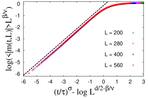
Figure 1: (Color online) Nonequilibrium-to-equilibrium scaling plot of magnetization at $T_{\rm c}=1.442987J/k_{\rm B}$ for $L=200$, $280$, $400$ and $560$ with $\beta/\nu=0.516$, $\sigma=0.47$ and $\tau_{m}=2.51$. All the data seem to be located on a single curve within this scale. The dashed line stands for the tangent $1$ as guides for eyes.

First, the scaling plot of magnetization (4) at the estimated critical temperature $T_{\rm c}=1.442987J/k_{\rm B}$ (to be explained later) with $\beta/\nu=0.516$, $\sigma=0.47$ and $\tau_{m}=2.51$ is displayed in Fig. 1, where all the data points for $L=200$ (averaged with $320,000$ random number sequences (RNS)), $280$ ($160,000$ RNS), $400$ ($80,000$ RNS) and $560$ ($80,000$ RNS) seems to be located on a single curve, as expected. Evaluation process of $T_{\rm c}$ and $\beta/\nu$ is shown in Fig. 2, where the data for $T=1.442984J/k_{\rm B}$, $1.442985J/k_{\rm B}$, $1.442987J/k_{\rm B}$, $1.442989J/k_{\rm B}$ and $1.442990J/k_{\rm B}$ (from bottom to top) in the saturation region are plotted with Eq. (4), and the data are almost on a single curve after the tuning of parameters. The finest scaling is observed at $T=1.442987J/k_{\rm B}$ with $\beta/\nu=0.516$, while deviations of the data at $T=1.442984J/k_{\rm B}$ with $\beta/\nu=0.511$ and at $T=1.442990J/k_{\rm B}$ with $\beta/\nu=0.519$ are not negligible. Since the direction of deviations is not systematic as varying the system size, these deviations cannot be reduced anymore. We take similar scaling plots for $1.442985J/k_{\rm B}\leq T\leq 1.442989J/k_{\rm B}$, and observe comparable scaling behaviors with gradually-varying exponent $0.512\leq\beta/\nu\leq 0.518$. The fine scaling behaviors for $T=1.442985J/k_{\rm B}\leq T\leq 1.442989J/k_{\rm B}$ becomes as bad as that at $T=1.442984J/k_{\rm B}$ by changing $\beta/\nu$ with $\pm 0.002$. Combining these results, we can safely conclude

$$T_{\rm c}=1.442987(2)J/k_{\rm B},\ \beta/\nu=0.515\pm 0.005.$$ (5)

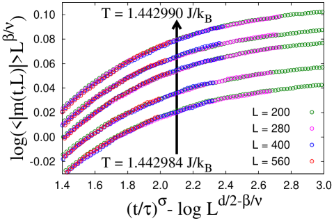
Figure 2: (Color online) Enlarged plot in the vicinity of equilibrium corresponding to Fig. 1 at $T=1.442984J/k_{\rm B}$, $1.442985J/k_{\rm B}$, $1.442987J/k_{\rm B}$, $1.442989J/k_{\rm B}$ and $1.442990J/k_{\rm B}$ with $\beta/\nu=0.511$, $0.512$, $0.516$, $0.518$ and $0.519$, respectively. Error bars are smaller than symbols.

When we fit the data for $L=560$ at $T_{\rm c}$ directly with Eq. (3), we have $\sigma\approx 0.49$, which is consistent with that of the 3D XY model Nono-letter and the exponent $\sigma\approx 1/2$ might be common in all the vector spin models characterized by the second-order phase transition. In this fitting the initial $\sim 50$ MCS data are used by minimizing the residue per data Nonomura14 . With this exponent the data between the stretched-exponential and equilibrium regions are not scaled so well as those plotted in Fig. 1 due to higher-order correction of simulation time, and the deviation from $\sigma=1/2$ may compensate such higher-order correction numerically.

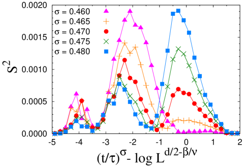
Figure 3: (Color online) Average mutual variance of the scaling plot in Fig. 1 for $\sigma=0.460$ (triangles), $0.465$ (crosses), $0.470$ (circles), $0.475$ (x-marks) and $0.480$ (squares). Overall variance seems to be the smallest for $\sigma\approx 0.47$.

Evaluation process of $\sigma$ is given in Fig. 3, which exhibits the average mutual variance $S^{2}$ in the scaling plot like Fig. 1 at $T_{\rm c}=1.442987J/k_{\rm B}$ for $\sigma=0.460$ (triangles), $0.465$ (crosses), $0.470$ (circles), $0.475$ (x-marks) and $0.480$ (squares). After the optimization of parameters $\beta/\nu$ and $\tau_{m}$ with given $\sigma$ for $L=200$, $280$, $400$ and $560$, variance of the data between different $L$ at the same scaled simulation time $t_{\ast}\equiv(t/\tau_{m})^{\sigma}-\log L^{d/2-\beta/\nu}$ (between the law data for one size and the linearly-interpolated ones for other sizes) is averaged in the width $\Delta t_{\ast}=0.2$ (for example, from $t_{\ast}=-5.0$ to $-4.8$).

Apparently, the variance is very small at the onset of ordering ($t_{\ast}\approx-5$) and in the vicinity of equilibrium ($t_{\ast}\approx 2$), and has two main peaks on the edge of the stretched-exponential ordering ($-3<t_{\ast}<-1$; region A) and between the stretched-exponential and equilibrium regions ($-1<t_{\ast}<1$; region B). For $\sigma=0.48$, the variance is the smallest in the region A while the largest in the region B, and vice versa for $\sigma=0.46$. For $\sigma=0.47$ the variance takes medium values in the both regions and these two values are almost the same, and therefore the most suitable within these three values. Behaviors for $\sigma=0.475$ and $0.465$ just locate in between. Optimized parameters are $\beta/\nu=0.515$ and $\tau_{m}=2.31$ for $\sigma=0.46$, and $\beta/\nu=0.517$ and $\tau_{m}=2.74$ for $\sigma=0.48$. That is, the variance of $\beta/\nu$ is much smaller than that of $\sigma$.

Calculations for the variance of the next order of $\sigma$ are affected by the precision of optimization of parameters or the method of interpolation (linear or up to higher orders). Such efforts may not be productive, because error bars in $\beta/\nu$ are smaller than those from the scaling analysis in Fig. 2 ($\pm 0.002$) for each temperature. Then, here we evaluate this exponent as $\sigma=0.47(1)$ and use this estimate for analyses of other physical quantities.

III.3 Evaluation of $\gamma/\nu$ from magnetic susceptibility

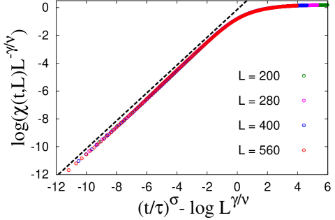
Figure 4: (Color online) Nonequilibrium-to-equilibrium scaling plot of magnetic susceptibility at $T_{\rm c}=1.442987J/k_{\rm B}$ for $L=200$, $280$, $400$ and $560$ with $\gamma/\nu=1.970$, $\sigma=0.47$ and $\tau_{\chi}=0.584$. All the data seem to be located on a single curve, and the dashed line stands for the tangent $1$ as guides for eyes.

Although evaluation of $T_{\rm c}$ based on the magnetic susceptibility is also possible, here we use $T_{\rm c}$ based on magnetization and estimate $\gamma/\nu$ similarly to the scheme used in Fig. 2. First, the magnetic susceptibility at $T_{\rm c}$ in the SW algorithm shows the stretched-exponential ordering,

$$\chi(t,L)\equiv\frac{1}{L^{d}}\sum_{i,j}\langle\vec{S}_{i}\cdot\vec{S}_{j}\rangle\sim\exp\left[+(t/\tau_{\chi})^{\sigma}\right].$$ (6)

This physical quantity has no size-dependent prefactor because duplicated random-walk growth of clusters ($\sim L^{-(d/2)\times 2}$) is cancelled with bulk response ($\sim L^{d}$). Since equilibrium value of this quantity is scaled as $\chi_{\rm c}\sim L^{\gamma/\nu}$, we have the following scaling form similar to Eq. (4),

$$\log(\chi(t,L)L^{-\gamma/\nu})\sim(t/\tau_{\chi})^{\sigma}-\log L^{\gamma/\nu}.$$ (7)

The scaling plot at $T_{\rm c}=1.442987J/k_{\rm B}$ with $\gamma/\nu=1.970$, $\sigma=0.47$ and $\tau_{\chi}=0.584$ is displayed in Fig. 4, where all the data points for $L=200$, $280$, $400$ and $560$ seems to be located on a single curve again. The data in the vicinity of equilibrium is shown in Fig. 5, together with the data for $T=1.442985J/k_{\rm B}$ (with $\gamma/\nu=1.977$) and $1.442989J/k_{\rm B}$ (with $\gamma/\nu=1.967$). Discrepancy from such scaling behaviors becomes clear by changing $\gamma/\nu$ with $\pm 0.002$. Combining these results, we conclude

$$\gamma/\nu=1.972\pm 0.007.$$ (8)

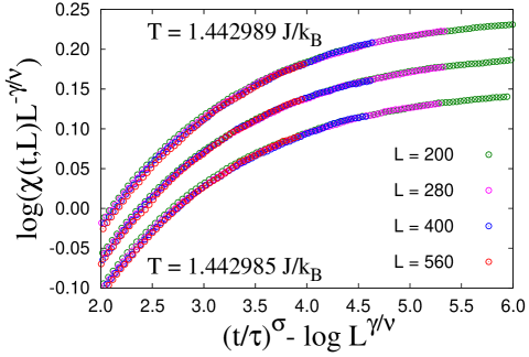
Figure 5: (Color online) Enlarged plot in the vicinity of equilibrium corresponding to Fig. 4 at $T=1.442985J/k_{\rm B}$, $1.442987J/k_{\rm B}$ and $1.442989J/k_{\rm B}$ with $\gamma/\nu=1.977$, $1.970$ and $1.967$, respectively. Error bars are smaller than symbols.

III.4 Evaluation of $\nu$ from temperature derivative of magnetization and $\alpha$ from scaling relation

Figure 6: Time dependence of the reversed temperature derivative of magnetization $\mu(t)$ at $T_{\rm c}=1.442987J/k_{\rm B}$ for $L=560$.

As explained in the Overview part of this section, the quantity $\mu(t)\equiv-{\rm d}\langle|m(t)|\rangle/{\rm d}T$ might be suitable for evaluation of $\nu$. Using the Hamiltonian of the model (1) as the energy variable, this quantity is expressed as

$$\mu(L)=-\frac{1}{T^{2}}\left(\langle|m|{\cal H}\rangle-\langle|m|\rangle\langle{\cal H}\rangle\right).$$ (9)

This expression is nothing but the subtraction between two nearly-equal quantities. Although the error bar is expected to be large in equilibrium, early-time behaviors from the perfectly-disordered state might be different, and law data of time dependence of $\mu(t)$ for $L=560$ averaged with $80,000$ RNS is displayed in Fig. 6.

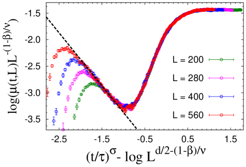
Figure 7: (Color online) Nonequilibrium-to-equilibrium scaling plot of the quantity $\mu(t,L)$ at $T_{\rm c}=1.442987J/k_{\rm B}$ for $L=200$, $280$, $400$ and $560$ with $(1-\beta)/\nu=0.889$, $\sigma=0.47$ and $\tau_{\mu}=7.40$. All the data except for the initial rapidly-increasing ones seem to be located on a single curve, and the dashed line stands for the tangent $-1$ as guides for eyes.

The quantity $\langle|m|{\cal H}\rangle$ monotonically decreases from zero as the simulation time increases, and it reaches $\sim-7\times 10^{6}$ at $t=225$ MCS for $L=560$. That is, $\mu(t)$ is obtained from the subtraction between two quantities of order of $\sim 10^{5}$ times larger. We may call the error bar of $\mu(t)$ rather “small” even for such severe calculations. This figure also reveals that the time dependence of $\mu(t)$ is quite nontrivial: It takes negative values in initial several steps, increases rapidly, arrives at a maximal value and gradually decreases, shows upturn again and finally saturates toward equilibrium. It is not possible to decide which region corresponds to the stretched-exponential time evolution a prior, and we have attempted some trials and investigated which assumption results in fine scaling behaviors in a wide parameter region.

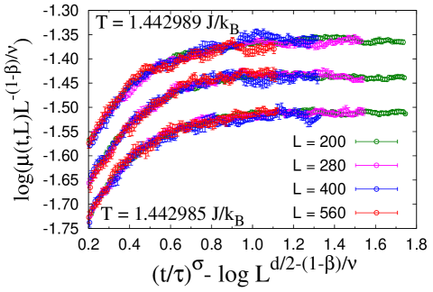
Figure 8: (Color online) Enlarged plot in the vicinity of equilibrium corresponding to Fig. 7 at $T=1.442985J/k_{\rm B}$, $1.442987J/k_{\rm B}$ and $1.442989J/k_{\rm B}$ with $(1-\beta)/\nu=0.890$, $0.889$ and $0.888$, respectively. Error bars are a few times larger than symbols, which exhibits large fluctuation of the data.

We finally find that the stretched-exponential decay before the upturn seems reasonable,

$$\mu(t,L)\sim L^{d/2}\exp[-(t/\tau_{\mu})^{\sigma}],$$ (10)

where the size dependence is derived by multiplying random-walk growth of clusters and bulk response. From Eq. (10) and the size dependence in equilibrium, $\mu_{\rm c}(L)\sim L^{(1-\beta)/\nu}$, we have the following scaling form,

$$\log(\mu(t,L)L^{-(1-\beta)/\nu})\sim(t/\tau_{\mu})^{\sigma}-\log L^{d/2-(1-\beta)/\nu}.$$ (11)

The scaling plot at $T_{\rm c}=1.442987J/k_{\rm B}$ with $(1-\beta)/\nu=0.889$, $\sigma=0.47$ and $\tau_{\mu}=7.40$ is displayed in Fig. 7, where all the data points except for the initial rapidly-increasing ones for $L=200$, $280$, $400$ and $560$ seems to be located on a single curve. Actually, the stretched-exponential scaling region is rather narrow and precise evaluation of $\tau_{\mu}$ is difficult from these data. Then, we fit this parameter with the data after the upturn, and confirm the acceptable stretched-exponential scaling with this estimate afterwards. The data in the vicinity of equilibrium is shown in Fig. 8, together with the data for $T=1.442985J/k_{\rm B}$ (with $(1-\beta)/\nu=0.890$) and $1.442989J/k_{\rm B}$ (with $(1-\beta)/\nu=0.888$). Discrepancy from such scaling behaviors becomes clear by changing $(1-\beta)/\nu$ with $\pm 0.005$, and we have $(1-\beta)/\nu=0.889(6)$. Combining this estimate with Eq. (5), we arrive at

$$1/\nu=1.404\pm 0.008\ \ {\rm or}\ \ \nu=0.712\pm 0.004.$$ (12)

Furthermore, when this estimate is coupled with the hyperscaling relation, $2-\alpha=d\nu$, we have

$$\alpha=-0.136\pm 0.012\ \ {\rm or}\ \ \alpha/\nu=-0.192\pm 0.016.$$ (13)

III.5 Complementary evaluation of $\alpha/\nu$ from specific heat and $\nu$ from scaling relation

The specific heat is expressed as

$$C(L)=\frac{1}{L^{d}T^{2}}\left(\langle{\cal H}^{2}\rangle-\langle{\cal H}\rangle^{2}\right).$$ (14)

This expression is also the subtraction between two nearly-equal quantities, of order of $\sim 10^{7}$ times larger than $C(L)$ itself in the vicinity of equilibrium for $L=560$. Although this ratio is even larger than that of $\mu(L)$, error bars of $C(L)$ are smaller than those of $\mu(L)$, because fluctuation of energy is much smaller than that of magnetization. Although time dependence of this quantity is essentially the same as that of $\mu(t)$ in Fig. 6, the stretched-exponential decay of this quantity is quite apparent (as will be shown in Fig. 9),

$$C(t,L)\sim L^{d}\exp\left[-(t/\tau_{C})^{\sigma}\right],$$ (15)

where the size dependence originates from bulk response. Combining this scaling form with the equilibrium finite-size scaling $C_{\rm c}(L)\sim L^{\alpha/\nu}$, we arrive at

$$\log(C(t,L)L^{-\alpha/\nu})\sim(t/\tau_{C})^{\sigma}-\log L^{d-\alpha/\nu}.$$ (16)

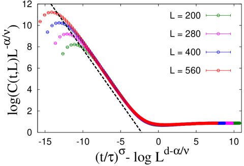
Figure 9: (Color online) Nonequilibrium-to-equilibrium scaling plot of specific heat at $T_{\rm c}=1.442987J/k_{\rm B}$ for $L=200$, $280$, $400$ and $560$ with $\alpha/\nu=0.074$, $\sigma=0.47$ and $\tau_{C}=0.215$. All the data except for initial several steps and those during the upturn seem to be located on a single curve, and the dashed line stands for the tangent $-1$ as guides for eyes.

The scaling plot at $T_{\rm c}=1.442987J/k_{\rm B}$ with $\alpha/\nu=0.074(5)$, $\sigma=0.47$ and $\tau_{C}=0.215$ for $L=200$, $280$, $400$ and $560$ is given in Fig. 9. The enlarged data after the upturn is shown in Fig. 10 together with the data for $T=1.442985J/k_{\rm B}$ and $1.442989J/k_{\rm B}$ with $\alpha/\nu=0.077(6)$ and $0.070(5)$, respectively. Error bars of the data are a bit larger than symbols, and error bars of estimates of the critical exponent $\alpha/\nu$ are also larger than those in other exponents. Combining these results we have $\alpha/\nu=0.074\pm 0.009$, and $\nu=0.651\pm 0.002$ from the hyperscaling relation. This estimate is not at all consistent with the one in Eq. (12), and such discrepancy had already been discussed in the 3D Heisenberg model Holm93 ; Brown96 ; Holm97 ; Kim00 ; Brown06 .

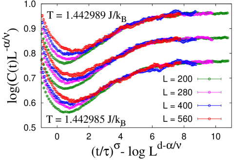
Figure 10: (Color online) Enlarged plot in the vicinity of equilibrium corresponding to Fig. 9 at $T=1.442985J/k_{\rm B}$, $1.442987J/k_{\rm B}$ and $1.442989J/k_{\rm B}$ with $\alpha/\nu=0.077$, $0..074$ and $0.070$, respectively. Error bars are a bit larger than symbols. This figure exhibits fluctuation of the data near equilibrium and large deviation of the data during the upturn.

In equilibrium simulations, such a puzzle of the specific heat is known to be resolved by dividing it to the regular and scaling parts as $C(L)=C_{\rm reg}-aL^{\alpha/\nu}$ Holm93 . In the present case, we should also consider time dependence of $C(L)$, namely the stretched-exponential scaling given in Eq. (15). Now we interpret this form as an alternative definition of the scaled simulation time $t_{\ast}\equiv(t/\tau_{C})^{\sigma}-\log L^{d}$, and the parameter $\tau_{C}$ is determined as the minimum of $C(t,L)$ to be independent of system size as shown in Fig. 11(a), which corresponds to $\tau_{C}\approx 0.27$.

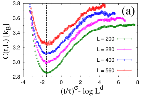
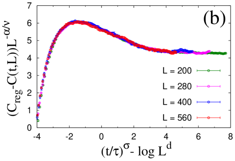
Figure 11: (Color online) (a) Specific heat at $T_{\rm c}=1.442987J/k_{\rm B}$ for $L=200$, $280$, $400$ and $560$ plotted versus the scaled simulation time $t_{\ast}\equiv(t/\tau_{C})^{\sigma}-\log L^{d}$ derived from the stretched-exponential scaling form (15). The parameter $\tau_{C}\approx 0.27$ is determined as the minimum of the specific heat becomes independent of $L$ (emphasized by the dashed line). (b) Scaling of the specific heat including the regular part (17). Assuming $\alpha/\nu=-0.192$ obtained from the scaling behavior of $\mu(t)$ in Eq. (13) and tuning $C_{\rm reg}\approx 5.05k_{\rm B}$, the coefficient of the scaling part of the specific heat becomes independent of $L$ in the whole region satisfying $C_{\rm reg}>C(t,L)$.

Now we assume that the regular part of the specific heat is independent of simulation time $t$, while the coefficient of the scaling part depends on $t$ as

$$C(t,L)=C_{\rm reg}-a(t)L^{\alpha/\nu}.$$ (17)

The point of this formulation is that $C_{\rm reg}>C(t,L)$ or $a(t)>0$ is satisfied in the scaling region, and that the exponent $\alpha$ can be negative even though $C(t,L)$ increases as the linear size $L$ increases. Although it is possible to estimate $C_{\rm reg}$ and $\alpha/\nu$ from the scaling plot based on Eq. (17) in principle, error bars of the estimates must be much larger than that of Eq. (13), because there exists an extra fitting parameter $C_{\rm reg}$ while the fluctuation of the data is comparable to that of $\mu(t,L)$.

Then, we only evaluate $C_{\rm reg}$ by assuming the exponent given in Eq. (13) and confirm the validity of the scaling (17). In Fig. 11(b), the quantity $(C_{\rm reg}-C(t,L))L^{-\alpha/\nu}$ is plotted versus the scaled simulation time with $C_{\rm reg}\approx 5.05k_{\rm B}$ at $T_{\rm c}=1.442987J/k_{\rm B}$ for $L=200$, $280$, $400$ and $560$, namely the $t_{\ast}$-dependence of the coefficient of the scaling part $a(t)$. Apparently, the scaling behavior in Fig. 11(b) seems much better than that in Fig. 10, or the improved scaling form (17) with negative $\alpha$ might be better than the naive scaling form (16) with positive $\alpha$.

IV Discussion

First, combining the scaling relation $\alpha+2\beta+\gamma=2$ and the hyperscaling relation, we have $2\beta/\nu+\gamma/\nu=d$. On the other hand, from Eqs. (5) and (8) we result in $2\beta/\nu+\gamma/\nu=3.002\pm 0.012$. That is, the critical exponent $\alpha/\nu$ can be evaluated from the temperature derivative of the magnetization without the hyperscaling relation, which is not so trivial as other scaling relations.

Refs.	Method	$\beta$	$\gamma$	$\nu$
present I	MC	$0.367(4)$	$1.404(9)$	$0.712(4)$
present II	MC	$0.367(2)$	$1.403(6)$	$0.712(3)$
Holm93 (1993)	MC	$0.362(3)$	$1.389(14)$	$0.704(6)$
Hasenbusch01 (2001)	MC	$0.3685(11)$	$1.393(4)$	$0.710(2)$
Campostrini02 (2002)	MC	$0.3691(6)$	$1.3957(22)$	$0.7113(11)$
Campostrini02 (2002)	MC+HTE	$0.3689(3)$	$1.3960(9)$	$0.7112(5)$
Butera97 (1997)	HTE (sc)	$0.3710(13)$	$1.406(3)$	$0.716(2)$
Butera97 (1997)	HTE (bcc)	$0.3700(13)$	$1.402(3)$	$0.714(2)$
Yukalov98 (1998)	$\epsilon$-Exp.	$0.367$	$1.39$	$0.708$
Guida98 (1998)	$\epsilon$-Exp.	$0.3655(35)$	$1.382(9)$	$0.7045(55)$
Guida98 (1998)	$d=3$ Exp.	$0.3662(25)$	$1.3895(50)$	$0.7073(35)$
Jasch01 (2001)	$d=3$ Exp.	$0.3655(5)$	$1.3882(10)$	$0.7062(7)$

Table 1: List of critical exponents estimated in the present study and in several previous numerical studies.

Next, we compare the estimates of $\beta$, $\gamma$ and $\nu$ obtained from Eqs. (5), (8) and (12) (present I) with several previous studies based on the Monte Carlo method Holm93 ; Hasenbusch01 ; Campostrini02 , high-temperature expansion Campostrini02 ; Butera97 , $\epsilon$-expansion Yukalov98 ; Guida98 or $d=3$ expansion Guida98 ; Jasch01 in Table 1. More comprehensive list of references was given in Ref. Campostrini02 . Note that our estimates shown above are based on “safe” evaluation. That is, the critical exponents are determined in order to cover the whole possible range of the critical scaling. If we assume that $T_{\rm c}$ locates in the middle of the scaling region and the critical exponents are evaluated just at $T_{\rm c}=1.442987(1)J/k_{\rm B}$, reasonable reduction of error bars is possible (present II).

From this table we may at least conclude that the estimates of critical exponents in the present study are consistent with those in previous studies, even though error bars are not so small. The dominant origin of statistical errors in our estimates is large fluctuations of $\mu(t,L)$. Since all the critical exponents evaluated with finite-size scaling analyses are scaled by $\nu$, Precision of this exponent is crucial. Nevertheless, the main purpose of the present study is to confirm the nontrivial stretched-exponential critical scaling in the 3D Heisenberg model, and evaluation of the critical exponents is not more than consistency check of this alternative scheme.

Actually, information of the critical exponents is not included in the stretched-exponential critical scaling of physical quantities in itself. Such information is introduced from the finite-size scaling of physical quantities in equilibrium, and the nonequilibrium-to-equilibrium scaling scheme enables to extract such information from the off-scaling data prior to equilibrium behaviors. The most promising application of the present scheme is to characterize phase transitions with nonequilibrium behaviors. In the standard NER scheme based on the local-update algorithms, power-law behaviors take place in general even in the BKT Ozeki-BKT or first-order Ozeki-1st phase transitions, and such characterization was made in a different manner by assuming the nature of phase transitions in advance. The situation might be different in the present cluster NER scheme, and investigations along this direction is now in progress Nono-letter .

The stretched-exponential nonequilibrium critical scaling initially found in the 2D Ising model Nonomura14 is now conformed in the 3D Heisenberg model. The exponent of stretched-exponential time dependence $\sigma\approx 1/2$ seems consistent with that of the 3D XY model Nono-letter , while not consistent with that of the 2D or 3D Ising models, $\sigma\approx 1/3$ Nonomura14 ; Nono-full . Even though our simulations on 3D vector spin models are based on the “embedded-Ising-spin” formalism, the exponent $\sigma$ is different from that of the Ising models. That is, this exponent is not determined by mere formalism, but by fundamental physical properties. Further details of such universal behaviors of the exponent $\sigma$ will be explained elsewhere Nono-full .

V Summary

Critical behaviors of the 3D Heisenberg model are investigated with the nonequilibrium ordering from the perfectly-disordered state in the Swendsen-Wang (SW) algorithm characterized by the stretched-exponential critical scaling form. Calculations from the perfectly-ordered state in the SW algorithm result in larger initial-time deviation and slower off-critical deviation, and those from the perfectly-disordered state in the Wolff algorithm show a power-law behavior similar to that in local-update algorithms. From simulations based on the “embedded-Ising spin” formalism we have the nonequilibrium-to-equilibrium scaling similarly to the 3D XY model, and all the data for $L=200$, $280$, $400$ and $560$ seem to be on a single curve in the whole simulation-time region with the stretched-exponential exponent $\sigma=0.47(1)$.

Precise values of the critical temperature and the critical exponent $\beta/\nu$ are evaluated simultaneously from the scaling analysis of the magnetization. Similarly, the critical exponent $\gamma/\nu$ is obtained from the scaling analysis of the magnetic susceptibility. The critical exponent $\nu$ is evaluated from the scaling analysis of the temperature derivative of magnetization, and the critical exponent $\alpha<0$ can be derived from the hyperscaling relation. A consistent estimate of $\alpha/\nu$ can be obtained from the specific heat by assuming the scaling form with the size-independent regular part and the negative scaling part.

Although information on standard critical behaviors such as the critical exponents is not included in the stretched-exponential critical scaling behaviors, such information can be extracted from off-scaling behaviors with the nonequilibrium-to-equilibrium scaling scheme, and the critical exponents comparable to previous studies can be obtained from the present framework without full equilibration.

Appendix A Evaluation of critical temperature from single system

A.1 Double-log plot

The simplest way to evaluate the critical temperature $T_{\rm c}$ from the early-time dependence of magnetization (2) or (3) is the double-log plot. When both sides of these equations are divided by the coefficient of rhs (expressed as $C$) and take logarithm twice, we have

$$\log(\log(\langle|m(t)|\rangle/C))\sim\mp\sigma\log(t/\tau_{m}).$$ (18)

Since Eq. (2) is obtained by relaxation from the perfectly-ordered state, the coefficient $C$ is of order of unity, and a naive plot assuming $C\equiv 1$ may be satisfactory enough. On the other hand, Eq. (3) is obtained by ordering from the perfectly-disordered state, and the small coefficient $C$ should be taken into account explicitly.

Practically, the unknown parameter $C$ can be determined by aligning the early-time data on a straight line, as shown in Fig. 12(a) with the data for $L=100$ with $2,000$ RNS in the SW algorithm from the perfectly-disordered state. Apparently, the ordering process in the double-log plot is faster or slower than linear for $T\leq 1.44J/k_{\rm B}$ or $T\geq 1.45J/k_{\rm B}$, respectively, which means $1.44J/k_{\rm B}<T_{\rm c}<1.45J/k_{\rm B}$. Tangent of the dashed line is $0.5$, which is consistent with $\sigma\approx 0.5$. Then, the variance of temperatures is reduced of one order in Fig. 12(b) with the data for $L=200$ with $2,000$ RNS, which results in $T_{\rm c}\approx 1.443J/k_{\rm B}$ with $\sigma\approx 0.5$.

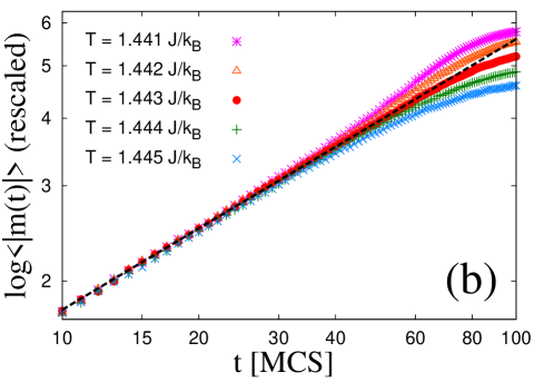
Figure 12: (Color online) Double-log plot of magnetization in the SW algorithm from the perfectly-disordered state for various temperatures around $T_{\rm c}$ for (a) $L=100$ and (b) $L=200$. The dashed line corresponds to the stretched-exponential ordering with $\sigma=0.5$.

Differently from the standard NER scheme based on the power-law behavior of physical quantities, the present scheme requires the rescaling of physical quantities with the unknown coefficient of stretched-exponential behaviors, and therefore precise evaluation of $T_{\rm c}$ is difficult.

A.2 Semi-log plot with fixed $\sigma$

If we intend to estimate more accurate $T_{\rm c}$ from the double-log plot, we may determine the linearity of the early-time data assuming the exponent $\sigma\equiv 0.5$. However, as long as $\sigma$ is fixed a prior, plotting $\log\langle|m(t)|\rangle$ versus $t^{\sigma}$ is more straightforward and precise, because no adjusting parameter other than $\sigma$ is included. Such semi-log plot with $\sigma\equiv 0.5$ is shown in Fig. 13(a) for $L=560$ with $10,000$ RNS around $T=1.443J/k_{\rm B}$. Evaluation of $T_{\rm c}$ is not an easy task because the data start deviating at $t=50\sim 60$ MCS, while they already begin to saturate at $t=70\sim 80$ MCS. Observing the data on the onset of deviation carefully, we may conclude $1.4429J/k_{\rm B}<T_{\rm c}<1.4430J/k_{\rm B}$.

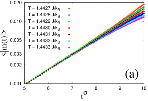
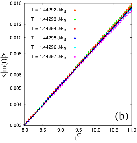
Figure 13: (Color online) Semi-log plot of magnetization versus $t^{\sigma}$ with $\sigma\equiv 0.5$ in the SW algorithm from the perfectly-disordered state for various temperatures around $T_{\rm c}$ for (a) $L=560$ and (b) $L=800$. The dashed line corresponds to $T_{\rm c}$ obtained from these figures. Discrepancy with the estimate in Section III reveals the limitation of this graphical scheme.

Then, the variance of temperatures is reduced of one more order in Fig. 13(b) with the data for $L=800$ with $5,000$ RNS. Although the data seem to suggest $1.44294J/k_{\rm B}<T_{\rm c}<1.44295J/k_{\rm B}$, this estimate of $T_{\rm c}$ is not consistent with the scaling plot given in Eq. (4) at all. Even though the data starts deviating at $t=80\sim 100$ MCS, they already begin to saturate in such simulation-time region. Downward-bending behavior due to saturation and upward-bending behavior below $T_{\rm c}$ are cancelled with each other in this region, and therefore $T_{\rm c}$ is underestimated when it is determined by the linearity of the nonequilibrium data. The scaling analysis explained in Section III is more reasonable and precise.

Appendix B Nonequilibrium relaxation from the perfectly-ordered state

B.1 Numerical results in the SW algorithm

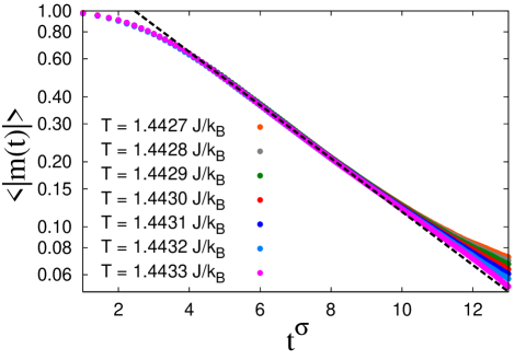
Figure 14: (Color online) Semi-log plot of magnetization versus $t^{\sigma}$ with $\sigma\equiv 0.5$ in the SW algorithm from the perfectly-ordered state for various temperatures around $T_{\rm c}$ for $L=560$. The dashed line emphasizes the region in which the stretched-exponential decay holds well, and it clarifies early-time rounding and saturation of data earlier than deviation induced by varying temperatures.

Relaxation data of magnetization from the perfectly-ordered state in the SW algorithm for $L=560$ with $400$ RNS are displayed in Fig. 14 with a semi-log plot versus $t^{\sigma}$, $\sigma\equiv 0.5$ similarly to Fig. 13. This figure shows merits and demerits of this scheme. First, although average number of RNS is one order smaller than that in Fig. 13, diversity of the data looks comparable. On the other hand, stable stretched-exponential decay only starts from $t\sim 20$ MCS as emphasized by the dashed line, while such behavior is observed from the beginning in Fig. 12. Moreover, the onset of deviation of the data induced by variance of temperature is $t\sim 80$ MCS, which is later than that in Fig. 13, and even later than the onset of saturation in Fig. 14, $t\sim 70$ MCS, which is comparable to that in Fig. 13. That is, evaluation of $T_{\rm c}$ from deviation of the data does not make sense, because this deviation is already affected by saturation behavior.

B.2 Numerical results in the Wolff algorithm

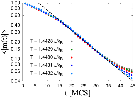
Figure 15: (Color online) Semi-log plot of magnetization in the Wolff algorithm from the perfectly-ordered state for various temperatures around $T_{\rm c}$ for $L=560$. The dashed line emphasizes the region in which the simple exponential decay holds well. Although time dependence looks similar to that in Fig. 14, we take $\sigma\equiv 1$ in this figure.

Relaxation data of magnetization from the perfectly-ordered state in the Wolff algorithm for $L=560$ with $100$ RNS are shown in Fig. 15 with a standard semi-log plot versus $t$, or the critical magnetization decays exponentially in this case. Similarly to the corresponding relaxation in the SW algorithm, stable exponential decay only starts from $t\sim 20$ MCS, and saturation of the data begins earlier than deviation induced by variance of temperature. Rather small number of RNS is due to larger numerical cost than that in the SW algorithm. Although required simulation time for equilibration looks much smaller than that in the SW algorithm, this time is scaled by the flipped cluster size in each step in the Wolff algorithm. Since the exponent $\beta/\nu$ is rather large ($\approx 0.5$) in the present model, the critical magnetization $m_{\rm c}(L)$ rapidly decreases as the linear size $L$ increases. This situation is quite different from that in the 2D Ising model Nonomura14 , where the small exponent $\beta/\nu=1/8$ ensured efficient update in the Wolff algorithm.

Aside from numerical efficiency, it is theoretically interesting that the exponent of the stretched-exponential decay (simple exponential decay can be regarded as the $\sigma=1$ case) depends on the species of the cluster algorithm. Such behaviors did not take place in the 2D Ising model Nonomura14 , where the decay exponent from the perfectly-ordered state is the same in the SW or Wolff algorithms. (Note that ordering behaviors from the perfectly-disordered state is quite different in the two algorithms even in the 2D Ising model Du .) Although the direction of flip is trivial in the Ising model, it is chosen randomly in the Heisenberg model. In each step the alignment is common in the whole system in the SW algorithm, but it is random from cluster to cluster in the Wolff algorithm. Absence of correlation between clusters is characteristic to behaviors above $T_{\rm c}$, and it results in the exponential decay. That is, the critical slowing down does not exist in the relaxation from the perfectly-ordered state in the Heisenberg model in the Wolff algorithm. Although this behavior is favorable for equilibration, it is not suitable for NER analyses.

References

- (1) R. H. Swendsen and J.-S. Wang, Phys. Rev. Lett. 58, 86 (1987).
- (2) F. Y. Wu, Rev. Mod. Phys. 54, 235 (1982).
- (3) P. W. Kasteleyn and C. M. Fortuin, J. Phys. Soc. Jpn. Suppl. 26, 11 (1969); C. M. Fortuin and P. W. Kasteleyn, Physica 57, 536 (1972).
- (4) U. Wolff, Phys. Rev. Lett. 62, 361 (1989).
- (5) D. W. Heermann and A. N. Burkitt, Physica A 162, 210 (1990).
- (6) C. F. Baillie and P. D. Coddington, Phys. Rev. B 43, 10617 (1991).
- (7) S. Gündüç, M. Dilaver, M. Aydin, and Y. Gündüç, Comp. Phys. Commun. 166, 1 (2005).
- (8) J. Du, B. Zheng, and J.-S. Wang, J. Stat. Mech. (2006), P05004.
- (9) Y. Nonomura, J. Phys. Soc. Jpn. 83, 113001 (2014).
- (10) As a recent review, Y. Ozeki and N. Ito, J. Phys. A 40, R149 (2007).
- (11) N. Ito, K. Hukushima, K. Ogawa, and Y. Ozeki, J. Phys. Soc. Jpn. 69, 1931 (2000); N. Ito, K. Ogawa, K. Hukushima, and Y. Ozeki, Prog. Theor. Phys. Suppl. 138, 555 (2000).
- (12) Since the scheme explained in Appendix A is used in Appendix B, the order of the appendices is reversed with the appearance in the main text.
- (13) Y. Nonomura and Y. Tomita, in preparation.
- (14) L. Schülke and B. Zheng, Phys. Lett. A 215, 81 (1996).
- (15) Y. Nonomura and Y. Tomita, in preparation.
- (16) C. Holm and W. Janke, Phys. Rev. B 48, 936 (1993).
- (17) R. G. Brown and M. Ciftan, Phys. Rev. Lett. 76, 1352 (1996).
- (18) C. Holm and W. Janke, Phys. Rev. Lett. 78, 2265 (1997).
- (19) J.-K. Kim, Phys. Rev. E 62, 8798 (2000).
- (20) R. G. Brown and M. Ciftan, Phys. Rev. B 74, 224413 (2006).
- (21) M. Hasenbusch, J. Phys. A 34, 8221 (2001).
- (22) M. Campostrini, M. Hasenbusch, A. Pelissetto, P. Rossi, and E. Vicari, Phys. Rev B 65, 144520 (2002).
- (23) P. Butera and M. Comi, Phys. Rev. B 56, 8212 (1997).
- (24) V. I. Yukalov and S. Gluzman, Phys. Rev. E 58, 1359 (1998).
- (25) R. Guida and J. Zinn-Justin, J. Phys. A 31, 8103 (1998).
- (26) F. Jasch and H. Kleinert, J. Math. Phys. 42, 52 (2001).
- (27) Y. Ozeki, K. Ogawa, and N. Ito, Phys. Rev. E 67, 026702 (2003).
- (28) Y. Ozeki, K. Kasono, N. Ito, and S. Miyashita, Physica A 321, 271 (2003).
- (29) M. Matsumoto and T. Nishimura, ACM TOMACS 8, 3 (1998). Further information is available from the Mersenne Twister Home Page, currently maintained by M. Matsumoto.