Quantum Spin Hall State on Square-like Lattice

Abstract

We find that quantum spin Hall (QSH) state can be obtained on a square-like or rectangular lattice, which is generalized from two-dimensional (2D) transition metal dichalcogenide (TMD) haeckelites. Band inversion is shown to be controled by hopping parameters and results in Dirac cones with opposite or same vorticity when spin-orbit coupling (SOC) is not considered. Effective k$\cdot$p model has been constructed to show the merging or annihilation of these Dirac cones, supplemented with the intuitive pseudospin texture. Similar to graphene based honeycomb lattice system, the QSH insulator is driven by SOC, which opens band gap at the Dirac cones. We employ the center evolution of hybrid Wannier function from Wilson-loop method, as well as the direct integral of Berry curvature, to identify the $Z_{2}$ number. We hope our detailed analysis will stimulate further efforts in searching for QSH insulators in square or rectangular lattice, in addition to the graphene based honeycomb lattice.

I Introduction

Topological insulator (TI) has attracted significant attentions from researchers in recent years. Hasan and Kane (2010); Qi and Zhang (2011); Bernevig and Hughes (2013); Weng et al. (2014a) Its bulk band structure is characterized by a global topological invariant $\mathbb{Z}_{2}$ number, Kane and Mele (2005a); Bernevig and Zhang (2006); Fu and Kane (2007a); Qi et al. (2006, 2008) which is protected by time-reversal (TR) symmetry. The bulk-boundary correspondence ensures that on the boundary of a TI there exists topologically protected metallic states which cross the bulk band gap by connecting the valence and conduction bands. Especially for two dimensional (2D) TI, the conducting one dimensional (1D) edge states have opposite velocity for opposite spin channel, which leads to quantum spin Hall (QSH) effect. Therefore, 2D TI is also known as QSH insulator. Since the backscattering of electrons in this 1D edge state is prohibited as long as TR symmetry is conserved, dissipationless quantized electron conductivity is expected and has great potential application as an ideal conducting wire in device.

However, up to now, only two materials have been confirmed by experimental observation of quantized conductivity inside of bulk band gap, namely, the quantum well structure composed of HgTe/CdTe K?nig et al. (2007) and InAs/GaSb. Knez et al. (2011) There have been intensive efforts in searching for 2D QSH insulator. One is based on the honeycomb lattice, which is stimulated by Kane-Mele model for graphene. Kane and Mele (2005a, b) The low-buckled silicene Liu et al. (2011), chemically decorated single layer honeycomb lattice of Sn, Xu et al. (2013) Ge Si et al. (2014) and Bi or Sb Song et al. (2014) are all in this category. The second category is represented by ZrTe₅/HfTe₅ Weng et al. (2014b) and Bi₄Br₄ Zhou et al. (2014). They are single layer exfoliated from their three-dimensional (3D) counterparts, which are weakly bonded layered materials. The proposal of 1T’ structure of single layer transition-metal dichalcogenide (TMD) Qian et al. (2014) can be ascribed to this type also. The third category are based on square or rectangular lattice. Such as recent proposals of 2D buckled square lattice BiF Luo and Xiang (2015) and rectangular TMD haeckelites. Nie et al. ; Sun et al. (2015); Ma et al. (2015)

In this work, we will discuss the possible topologically nontrivial quantum states based on the model built for 2D monolayer transition metal dichalcogenide (TMD) haeckelites, Li et al. (2014); Terrones and Terrones (2014) among which MX₂ (M=Mo, W and X=S, Se, Te ) have been predicted to be QSH insulators by Nie et al. Nie et al. , Sun et al. Sun et al. (2015) and Ma et al. Ma et al. (2015) using first-principles calculations.

The paper is organized as follows. In section II,the effective tight-binding (TB) model of TMD haeckelites are constructed from symmetrical analysis. In section III, the symmetry and topology of the lattice model and the topological phase transition have been discussed. In section IV, the vorticity, merging or annihilation of Dirac cones have been demonstrated by k$\cdot$p model. In section V, we provide a brief summary.

II Derivation of Tight Binding Model

Monolayer of TMD in its top view, such as MoS₂, can be thought as a honeycomb lattice with Mo and S on the A and B sublattice site, respectively. However, recently a kind of ordered square-octagonal distortion have been introduced in honeycomb TMD to form haeckelite structure Li et al. (2014); Terrones and Terrones (2014) as that in graphene. Such TMD haeckelites have pairs of square-octagon composed of M and X atoms, noted as MX₂-4-8 to be distinguished from usual MX₂ with honeycomb lattice. In our previous work Nie et al. , the first-principles calculation for WS₂-4-8 indicates the four bands around the Fermi level are mainly contributed by $d_{z^{2}}$ orbitals of M atoms. The $p$ orbitals from X atoms are quite far from Fermi level and can be safely ignored. In this point of view, the square-octagonal lattice can be further simplified to be a rectangular lattice with only four M atoms per unit cell as shown in Fig.  1.

II.1 Hamiltonian without SOC Term

We take $d_{z^{2}}$ orbital on each M atom as local orbital basis and note it as Wannier orbital $w_{n}(\bm{r}-\bm{R}_{l})$. Here $n$=1…4 indicates four nonequivalent M atoms in one unit cell as shown in Fig. 1 and $\bm{R}_{l}$ is the lattice index. Such rectangular lattice has space group $Pbam$ and the following symmetries are satisfied.

$\mathcal{P}$

inversion symmetry operator. M₁ (M₂) and M₃ (M₄) are related by $\mathcal{P}$.

$m_{z}$

mirror operator with mirror plane perpendicular to normal of the 2D lattice plane. All M atoms keep identity.

$\left\{C_{2x}|\frac{1}{2}\frac{1}{2}0\right\}$

This is a non-symmorphic operation. After $C_{2}$ rotation around $x$-axis (along a lattice), a glide of $(\frac{1}{2},\frac{1}{2},0)$ (in unit of lattice vectors) is applied. This operation relates M₁ (M₃) with M₂ (M₄).

Therefore, there are only three independent hopping terms in tight-binding (TB) approximation and they are:

$$t_{1}=\langle w_{1}|H_{0}|w_{2}\rangle$$ (1)

$$t_{2}=\langle w_{1}|H_{0}|w_{3t}\rangle$$ (2)

$$t_{3}=\langle w_{1}|H_{0}|w_{4}\rangle$$ (3)

Here $H_{0}$ is the Hamiltonian of system without considering of spin-orbit coupling (SOC). The hopping parameters $t_{1}$, $t_{2}$ and $t_{3}$ are marked in Fig. 1 also. All these parameters must be real because $w_{n}$ and $H_{0}$ are real. After fourier transformation $H_{0nm}(\bm{k})=\sum_{\bm{R}}\langle w_{n}(0)|H_{0}|w_{m}(\bm{R})\rangle e^{i\bm{k}\cdot\bm{R}}$, we get $\bm{k}$ dependent Hamiltonian $H_{0}(\bm{k})$ satisfying periodic condition $H_{0}(\bm{k})$=$H_{0}(\bm{k+G})$ with $\bf{G}$ being integer times of reciprocal lattice. A $\bf{k}$-dependent gauge transformation $H_{0}(\bm{k})\to U(\bm{k})H_{0}(\bm{k})U^{\dagger}(\bm{k})$ is applied to get a concise but not periodic form of $H_{0}(\bm{k})$ in Eq. (8). This form is more convenient for deriving the effective k$\cdot$p models used in section IV.

$$H_{0}(\bm{k}) =\left(\begin{array}[]{cccc}0&\gamma_{1}&\gamma_{2}^{-}&\gamma_{3}\\ \gamma_{1}^{*}&0&\gamma_{3}^{*}&\gamma_{2}^{+}\\ \gamma_{2}^{-*}&\gamma_{3}&0&\gamma_{1}\\ \gamma_{3}^{*}&\gamma_{2}^{+*}&\gamma_{1}^{*}&0\end{array}\right)$$ (8)

$$\gamma_{1} =2t_{1}\cos\left(\frac{k_{x}}{2}\right)$$

$$\gamma_{2}^{\pm} =t_{2}e^{-i\frac{1}{2}(k_{x}\pm k_{y})}$$

$$\gamma_{3} =2t_{3}\cos\left(\frac{k_{y}}{2}\right)$$

$$U(\bm{k})=\left(\begin{array}[]{cccc}1&0&0&0\\ 0&e^{-\frac{i}{2}k_{x}}&0&0\\ 0&0&e^{-\frac{i}{2}(k_{x}+k_{y})}&0\\ 0&0&0&e^{-\frac{i}{2}k_{y}}\end{array}\right)$$ (13)

II.2 Spin-Orbit Coupling Terms

To include SOC term, the degree of freedom of spin is introduced explicitly to expand the dimension of the Hamiltonian from four to eight. The spinor basis set is defined as:

$$|\phi_{i}\rangle =w_{i}(\bm{r})\otimes\chi_{\uparrow}\quad i=1\cdots 4$$ (14)

$$|\phi_{i+4}\rangle =w_{i}(\bm{r})\otimes\chi_{\downarrow}\quad i=1\cdots 4$$ (15)

, where $\chi_{\uparrow}$=$(1,0)^{T}$ and $\chi_{\downarrow}$=$(0,1)^{T}$ with $T$ representing transpose. Correspondingly, all the above symmetrical operators should be adjusted:

$$\mathcal{P}\to\mathcal{P}\\$$

$$m_{z}\to m_{z}e^{-\frac{i}{2}\pi\sigma_{z}}\\$$

$$\left\{C_{2x}|\frac{1}{2}\frac{1}{2}0\right\}\to\left\{C_{2x}|\frac{1}{2}\frac{1}{2}0\right\}e^{-\frac{i}{2}\pi\sigma_{x}}$$

and TR operator is defined as $\mathcal{T}=-i\sigma_{y}K$ with K is complex conjugation operator. Considering these symmetrical constraints, we will derive the term including SOC $H_{so}$.

Mirror symmetry $m_{z}$. Similar as the case in Kane-Mele modelKane and Mele (2005b) on honeycomb lattice without Rashba term, $H_{so}$ for present TMD haeckelite is also block diagonal in spin space because of $m_{z}$ symmetry. This can be proved as:

$$\forall i,j=1\cdots 4$$

$$\langle\phi_{i+4}|H_{so}|\phi_{j}\rangle =\langle m_{z}e^{-\frac{i}{2}\pi\sigma_{z}}\phi_{i+4}|H_{so}|m_{z}e^{-\frac{i}{2}\pi\sigma_{z}}\phi_{j}\rangle$$

$$=-\langle\phi_{i+4}|H_{so}|\phi_{j}\rangle=0$$

The derivation from the second line to the third line is due to $e^{-\frac{i}{2}\pi\sigma_{z}}=-i\sigma_{z}$.

Time-reversal symmetry $\mathcal{T}$. $H_{so}^{\uparrow\uparrow}$ and $H_{so}^{\downarrow\downarrow}$ are related by $\mathcal{T}$:

$$\langle\phi_{i+4}|H_{so}|\phi_{j+4}\rangle =\langle\mathcal{T}\phi_{i}|H_{so}|\mathcal{T}\phi_{j}\rangle$$

$$=\langle\phi_{j}|H_{so}|\phi_{i}\rangle$$ (16)

i.e., $H_{so}^{\uparrow\uparrow}=H_{so}^{\downarrow\downarrow T}$.

Inversion symmetry $\mathcal{P}$ and combined symmetry $\left\{C_{2x}|\frac{1}{2}\frac{1}{2}0\right\}e^{-\frac{i}{2}\pi\sigma_{x}}\cdot\mathcal{T}$. These two operations do not flip spin. After an intuitive graphic analysis as illustrated in Fig. 1, one can easily find that there are only two independent non-zero parameters:

$$\langle\phi_{1}|H_{so}|\phi_{2}\rangle =\langle\phi_{3}|H_{so}|\phi_{4}\rangle=i\lambda_{1}$$ (17)

$$\langle\phi_{1}|H_{so}|\phi_{4}\rangle =\langle\phi_{3}|H_{so}|\phi_{2}\rangle=i\lambda_{3}$$ (18)

Note that these two SOC terms must be pure imaginary numbers because $\phi_{i}$ are real and $H_{so}$ contains an imaginary unit. We also note that $\langle\phi_{1}|H_{so}|\phi_{3t}\rangle$ must be zero because $\mathcal{P}$ transforms it to its complex conjugation.

Therefore, $H_{so}$ is always diagonal in spin space and $\mathcal{PT}$ guarantees spin degeneracy, i.e., Kramer degeneracy. We only need to deal with $H_{so}^{\uparrow\uparrow}$ for the rest of this article. The concise matrix form of $H_{so}$ in Eq. (23) is achieved by the same gauge transform (Eq. (13)) performed to one spin channel of $H_{so}(\bm{k})$.

$$H_{so}^{\uparrow\uparrow}(\bm{k}) =\left(\begin{array}[]{cccc}0&\delta_{1}&0&\delta_{3}\\ \delta_{1}^{*}&0&\delta_{3}^{*}&0\\ 0&\delta_{3}&0&\delta_{1}\\ \delta_{3}^{*}&0&\delta_{1}^{*}&0\end{array}\right)$$ (23)

$$\delta_{1} =2i\lambda_{1}\cos\left(\frac{k_{x}}{2}\right)$$

$$\delta_{3} =2i\lambda_{3}\cos\left(\frac{k_{y}}{2}\right)$$

Now we get the total effective TB model $H(\bm{k})$=$H_{0}(\bm{k})+H_{so}(\bm{k})$, but keep in mind that the periodic condition is sacrificed to get the conciseness in Eq. (8) and Eq. (23), and a gauge transformation (Eq. (13)) to periodic form is needed when calculating properties concerning global phase such as Berry phase and related properties.

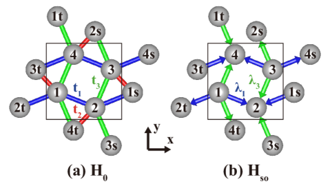
Figure 1: 2D rectangular lattice with four sties per cell. (a) Hopping parameters $t_{1}$, $t_{2}$ and $t_{3}$ in $H_{0}$. (b) Finite parameters $\lambda_{1}$ and $\lambda_{3}$ in $H_{so}$ with each arrow points from bra to ket.

III Symmetry and Topology of the Bands

From the analysis of symmetry in the above section, we obtain a TB model as shown in Eq. (8) and Eq. (23). We now focus on the band structure and the topology with different choice of related parameters. In real materials, these parameters are determined by details in crystal structure and choice of M and X elements in MX₂-4-8 haeckelites. Nie et al. It should be noticed that only the sign($t_{1}t_{2}t_{3}$) makes sense. This can be easily understood if we can use some unitary transformation $UHU^{T}$ to change $t_{i}$’s signs in pairs. For example, $U$=$\mathbb{I}_{2}\otimes\tau_{z}$ transforms $t_{1}$, $t_{3}$ to $-t_{1}$, $-t_{3}$ and $U$=$\tau_{z}\otimes\mathbb{I}_{2}$ transforms $t_{2}$, $t_{3}$ to $-t_{2}$, $-t_{3}$. The change in the $\text{sign}(t_{1}t_{2}t_{3})$, whatever which sign($t_{i}$) changes, is equivalent to $H_{0}(\bm{k})\to-H_{0}(\bm{k})$. Without loss of generality, in the rest of this paper we deal with $0<t_{3}\leq t_{1}$. For the case $|t_{1}|\leq|t_{3}|$, the system can be thought as the case $|t_{1}|\geq|t_{3}|$ with the interchange of $x$ and $y$ axes, which is apparent in Fig. 1. For clarity, we list all possible band structure with $0<t_{3}\leq t_{1}$ in Fig. 2. The classification and topology of them will be discussed in the following.

III.1 Symmetry of The Eigenstates

Table 1: Eigen energies, their degeneracy and eigenvalues of symmetrical operations of $H_{0}(\bm{k})$ at four time-reversal invariant momenta (TRIM).

	Energy	Folds	$\mathcal{P}$	$\{C_{2x}|\bm{\tau}_{x}\}$	$\{C_{2y}|\bm{\tau}_{y}\}$
$\Gamma$	$E_{A}^{0}=t_{2}-2(t_{1}+t_{3})$	1	1	-1	-1
	$E_{B}^{0}=-t_{2}-2(t_{1}-t_{3})$	1	-1	-1	1
	$E_{C}^{0}=-t_{2}+2(t_{1}-t_{3})$	1	-1	1	-1
	$E_{D}^{0}=t_{2}+2(t_{1}+t_{3})$	1	1	1	1
$X$	$-\sqrt{t_{2}^{2}+4t_{3}^{2}}$	2	$\pm 1$	$\pm 1$	$\pm 1$
	$\sqrt{t_{2}^{2}+4t_{3}^{2}}$	2	$\pm 1$	$\pm 1$	$\pm 1$
$Y$	$-\sqrt{t_{2}^{2}+4t_{1}^{2}}$	2	$\pm 1$	$\pm 1$	$\pm 1$
	$\sqrt{t_{2}^{2}+4t_{1}^{2}}$	2	$\pm 1$	$\pm 1$	$\pm 1$
$S$	$-t_{2}$	2	$1,1$	$\pm i$	$\pm i$
	$t_{2}$	2	$-1,-1$	$\pm i$	$\pm i$

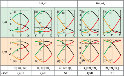
Figure 2: Band structure of $H_{0}(\bm{k})$ for all possible parameter choices with $0<t_{3}\leq t_{1}$. (a)-(f) and (g)-(j) show bands without ($t_{3}\neq t_{1}$) and with ($t_{3}=t_{1}$) $C_{4}$ symmetry, respectively. Upper and lower panels are for $t_{2}>0$ and $t_{2}<0$ cases, respectively. Color of each band represents its representation under the conserved non-symmorphic rotational symmetry. Along $\Gamma$-X ($\Gamma$-Y), black (green) and red (yellow) represent +1 and -1 eigenvalue of $\{C_{2x}|\frac{1}{2}\frac{1}{2}0\}$ ($\{C_{2y}|\frac{1}{2}\frac{1}{2}0\}$), respectively. Including SOC term will drive the system into QSH insulator or normal insulator (NI) as indicated for different parameter choice.

$H_{0}(\bm{k})$ at time-reversal invariant momenta (TRIM) Fu and Kane (2007b) can be solved analytically. The eigen energies, degeneracy and eigenvalue of symmetrical operators of the eigen states are listed in Table 1. Little group at $\Gamma$ of $Pbam$ has only one-dimensional irreducible representations,Aroyo et al. (2006) and all symmetrical operations can be diagonalized within the space spanned by eigen wavefunctions.

At TRIM $X(\pi,0,0)$ or $Y(0,\pi,0)$, $Pbam$ has only 2D irreducible representations. Within the eigen states of $H_{0}(\bm{k})$, they can be written as following:

$$D_{X}\left(\mathcal{P}\right)=D_{Y}(\mathcal{P}) =\begin{pmatrix}\tau_{3}&0\\ 0&\tau_{3}\end{pmatrix}$$ (24)

$$D_{X}\left(C_{2x}|\frac{1}{2}\frac{1}{2}0\right) =\begin{pmatrix}\tau_{2}&0\\ 0&\tau_{2}\end{pmatrix}$$ (25)

$$D_{Y}\left(C_{2y}|\frac{1}{2}\frac{1}{2}0\right) =\begin{pmatrix}\tau_{2}&0\\ 0&\tau_{2}\end{pmatrix}$$ (26)

in which $\tau_{i}$ denotes the $i$-th pauli matrix, representing the space spanned by two-fold degenerate eigenstates of $H_{0}(\bm{X})$ or $H_{0}(\bm{Y})$. We can character symmetry properties of each eigen space by eigenvalues of symmetrical operators. For example, the two-fold degenerate eigenstates at either $X$ (or $Y$) have even and odd parities respectively since inversion symmetry $\mathcal{P}$ is represented as $\tau_{3}$ (or $\tau_{2}$), thus we note this eigen space with $\pm 1$ in Table 1. Solutions at $S(\pi,\pi,0)$ are special. Little group of $Pbam$ at $S$ has only one-dimensional irreducible representations. However, for $\{C_{2x}|\frac{1}{2}\frac{1}{2}0\}$ and $\{C_{2y}|\frac{1}{2}\frac{1}{2}0\}$, the eigenvalues of the two eigenstates with the same parity are $\pm i$. Thus, the TR operator connects them and makes them two-fold degenerate.

From Table 1, we can see that the order of eigen energies at $X$ and $Y$ do not depend on the choice of $t_{i}$. Further, since the parities of the double degenerate states are always in pair, the band inversion at $X$ and $Y$ will not change the topology of the occupied bands. At $S$, the situation is similar, though the energy order depends on sign of $t_{2}$. Therefore, only the band inversion at $\Gamma$ can result in different topology of occupied bands. This is similar to large-band gap 2D topological insulator ZrTe₅. Weng et al. (2014b)

The order of energies at $\Gamma$ depends on $t_{i}$ explicitly as illustrated in Fig. 2. Along $\Gamma$-X(Y), $\{C_{2x}|\frac{1}{2}\frac{1}{2}0\}$ ($\{C_{2y}|\frac{1}{2}\frac{1}{2}0\}$) symmetry is conserved and the eigenstates with the same eigenvalue of $\{C_{2x}|\frac{1}{2}\frac{1}{2}0\}$ ($\{C_{2y}|\frac{1}{2}\frac{1}{2}0\}$) at different k points form a continuous band, which is identified by different color in Fig. 2. As long as $|t_{2}|<2t_{1}$, the $\{C_{2x}|\frac{1}{2}\frac{1}{2}0\}$ eigenvalues of the two lower bands at $\Gamma$ are $-1,-1$, while those at $X$ are $1,-1$. There must be a level crossing along $\Gamma$-X path. However, if $|t_{2}|>2t_{1}$ , the eigenvalues of the two lower bands at $\Gamma$ and $X$ are the same and so there is no crossing. But we’d like to remind that even without the above $C_{2}$ symmetry, as long as TR and $\mathcal{P}$ is conserved, such spineless 2D lattice model will have stable band crossing once band inversion happens. Weng et al. (2014); Yu et al. (2015) $C_{2}$ symmetry constraints the crossing point on the path along $\Gamma$-X or $\Gamma$-Y, which is similar to the spinless graphene model.Bernevig and Hughes (2013) A detailed discussion about these crossing points will be carried out in section IV.

III.2 Topological Phase

We now investigate whether a QSH insulating state can occur or not after SOC term is considered, which is similar to what happens in Kane-Mele model.Kane and Mele (2005b, a) The $\mathbb{Z}_{2}$ number of system with both TR and inversion $\mathcal{P}$ symmetries is determined by the product of parities of occupied states at four TRIM.Fu and Kane (2007b) SOC term opens band gap at the band crossing points as shown in Fig. 3(a). As long as $|t_{2}|<2\text{max}(t_{1},t_{3})$, $\mathbb{Z}_{2}$ number is 1 as shown in Fig. 2. To verify this we calculate the evolution of hybrid Wannier function centers for occupied bands using wilson loop method.Yu et al. (2011); Weng et al. (2014a) The plot is shown in Fig. 3(b). This illustrates that the winding number of two occupied bands is 1, indicating that the Chern number of spin up bands is 1. Due to TR symmetry, the spin down bands should have Chern number $-1$. Therefore, the model with $|t_{2}|<2\text{max}(t_{1},t_{3})$ and non-zero SOC parameter $\lambda_{i}$ is a QSH insulator state. For the case $|t_{2}|>2\text{max}(t_{1},t_{3})$, there will be no band inversion and the product of parities is 1, i.e., the system becomes a trivial normal insulator (NI).

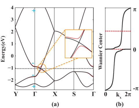
Figure 3: Bands and wannier centers’ evolution with SOC. (a) shows bands in which black lines denote non-SOC bands and red lines denote SOC bands. (b) shows wannier centers’ evolution of spin up electrons. The dashed red lines indicate reference lines. The parameters are set as $t_{1}=1$, $t_{2}=1.3$, $t_{3}=0.8$, $\lambda_{1}=-\lambda_{3}=0.04$.

Explicitly, we investigate the topological phase transition (TPT) between TI and NI driven by tuning one parameter $t_{2}$. Such TPT from QSH insulator to NI in centrosymmetric system will experience a gapless state with a Dirac node at TRIM. Murakami and Kuga (2008); Murakami (2011) As illustrated in Fig. 2, the TPT can be thought as the bands inversion of $A$ and $C$ at $\Gamma$ in case $t_{2}>0$ or $B$ and $D$ in case $t_{2}<0$. Hence, at TPT point the eigen energies of $H_{0}(\Gamma)+H_{so}(\Gamma)$ satisfy $E_{A}=E_{C}$ or $E_{B}=E_{D}$ with

$$E_{A} =t_{2}-2\sqrt{(t_{1}+t_{3})^{2}+(\lambda_{1}+\lambda_{3})^{2}}$$ (27)

$$E_{B} =-t_{2}-2\sqrt{(t_{1}-t_{3})^{2}+(\lambda_{1}-\lambda_{3})^{2}}$$ (28)

$$E_{C} =-t_{2}+2\sqrt{(t_{1}-t_{3})^{2}+(\lambda_{1}-\lambda_{3})^{2}}$$ (29)

$$E_{D} =t_{2}+2\sqrt{(t_{1}+t_{3})^{2}+(\lambda_{1}+\lambda_{3})^{2}}.$$ (30)

All of the corresponding eigen states are spin degenerate. It’s easy to find the critical value of $t_{2}$:

$$t_{2C}= \pm\sqrt{(t_{1}+t_{3})^{2}+(\lambda_{1}+\lambda_{3})^{2}}$$

$$\pm\sqrt{(t_{1}-t_{3})^{2}+(\lambda_{1}-\lambda_{3})^{2}}$$ (31)

Since $t_{2C}$ depends on $t_{i}$ and $\lambda_{i}$ ($i$=1 and 3), band inversion is influenced by both hopping effect and SOC in real materials.

IV Dirac points and quadratic band touching

From the above discussion, our model can be looked as an analog of graphene on a rectangular lattice: a significant resemblance is that QSH state occurs when SOC term opens gap at Dirac points. Since the lattice constants $a$ and $b$ are quite close to each other in previously studied TMD haeckelites, Nie et al. we’d like to go further to see what will happen in a square lattice with $C_{4}$ symmetry, which is the case studied in Ref. Li et al., 2014 and  Ma et al., 2015. We find that in square lattice the non-SOC band structure has a quadratic band touching at $\Gamma$, being different from the linear Dirac cones in graphene and rectangular lattice. As all interesting physics are related to the linear Dirac cone or the quadratic non-Dirac cone band touching, in this section we use effective k$\cdot$p model to characterize them. Alternatively, instead of calculating the evolution of centers of hybrid Wannier functions, Yu et al. (2011); Weng et al. (2014a) we calculate the integral of berry curvature analytically by treating $H_{so}$ as an infinity small perturbation term to identify the topological invariant.

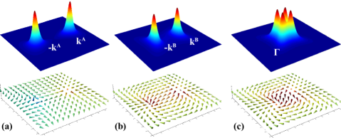
Figure 4: Berry curvature and pseudospin distribution in momentum space around around band crossing or touching points. (a) shows the Dirac cones with opposite vorticity. (b) and (c) show the Dirac cones having the same vorticity when $C_{4}$ symmetry is slightly broken and conserved , respectively.

IV.1 Linear Dirac Nodes in Rectangular lattice

As the non-trivial topology comes from band inversion of A, C or B, D bands around $\Gamma$, it’s natural to choose the states of A, C or B, D as the bases to establish k$\cdot$p model to capture the essence of the underlying physics. We take the case of A, C band inversion in the following discussion and the B and D inversion case can be easily inferred from it. We expand Eq. (8) and Eq. (23) to second order of $\bm{k}$ and then use the downfolding techniqueVoon and Willatzen (2009); Winkler (2003) to reduce the dimensionality in order to get the effective Hamiltonian in the bases of eigenstates $|A\rangle$ and $|C\rangle$. To keep the k$\cdot$p model similar to the Kane-Mele model, we transform $|A\rangle$ and $|C\rangle$ to the following two bases:

$$|1\rangle=\frac{-|w_{1}\rangle+|w_{4}\rangle}{\sqrt{2}}\qquad|2\rangle=\frac{|w_{2}\rangle-|w_{3}\rangle}{\sqrt{2}}$$ (32)

Within the above basis set, the space inversion and TR operators are

$$D_{AC}(\mathcal{P})=\tau_{1}\quad \text{and}~{}~{}~{}D_{AC}(K)=K$$ (33)

, respectively, both of which are the same as those in Kane-Mele model.

After some approximation (neglecting second order of $\lambda_{i}$), we get the k$\cdot$p model in basis set of $|1\rangle$ and $|2\rangle$:

$$H_{AC}(\bm{k}) =E_{AC}(\bm{k})+\left[t_{2}\left(2-\frac{1}{8}\bm{k}^{2}\right)-t_{1}\left(2-\frac{1}{4}k_{x}^{2}\right)+Fk_{x}^{2}\right]\tau_{1}-\frac{t_{2}}{2}k_{y}\tau_{2}+Jk_{x}\tau_{3}$$ (34)

$$F =\frac{t_{2}^{2}}{8(E_{A}-E_{B})}-\frac{t_{2}^{2}}{8(E_{C}-E_{D})}$$ (35)

$$J =-\frac{t_{2}}{4}\left[\frac{\Delta_{-}}{E_{A}-E_{B}}+\frac{\Delta_{-}}{E_{C}-E_{B}}+\frac{\Delta_{+}}{E_{A}-E_{D}}+\frac{\Delta_{+}}{E_{C}-E_{D}}\right]$$ (36)

where $E_{AC}(\bm{k})$ is an even function of $\bm{k}$ and $\Delta_{\pm}$ is defined as $\Delta_{\pm}=2(\lambda_{1}\pm\lambda_{3})$.

If SOC is not present, i.e., $\Delta_{\pm}$=0, there will be two Dirac cones from Eq. 34 and the location of the two nodes $\pm\bm{k}^{A}$ are determined by solution of $H_{AC}(\bm{k})=0$. $\bm{k}^{A}$ is found to be:

$$\bm{k}^{A} =\bm{e}_{1}\sqrt{\frac{2t_{1}-t_{2}}{F+(2t_{1}-t_{2})/8}}.$$ (37)

$\bm{e}_{1}$ is the unit vector along $\Gamma$-X path. In the case $t_{1}<t_{3}$, $\bm{k}^{A}$ is along $\Gamma$-Y. Expanding the hamiltonian Eq. 34 around $\bm{k}^{A}$ or $-\bm{k}^{A}$ to the lowest order of $\Delta_{\pm}$ and $\bm{q}$ (here a general $\bm{k}$ is $\pm\bm{k}^{A}$+$\bm{q}$), we get a linear dispersion hamiltonian, i.e. a Dirac hamiltonian:

$$H(\pm\bm{k}^{A}+\bm{q}) =\pm\alpha k_{1}^{A}q_{1}\tau_{1}-\frac{t_{2}}{2}q_{2}\tau_{2}\pm Jk_{1}^{A}\tau_{3}=\bm{d}\cdot\bm{\tau}$$ (38)

$$\alpha =\frac{2t_{1}-t_{2}}{4}+2F$$ (39)

Here $\bm{d}$=$(d_{1},d_{2},d_{3})$ and $\bm{\tau}$=$(\tau_{1},\tau_{2},\tau_{3})$. Representation of $\mathcal{P}K$ is $\tau_{1}K$ and $(\mathcal{P}K)^{-1}H(\bm{k})\mathcal{P}K=H(\bm{k})$ guarantees the mass term (the term proportional to $\tau_{3}$ ) to be zero. Therefore, $\bm{d}$ becomes a 2-component vector. The two Dirac cones possess opposite vorticity defined as $\mathrm{sign}(\det({\partial\bm{d}}/{\partial\bm{q}}))$. In this sense, any perturbation holds $\mathcal{P}K$ symmetry can only move the positions of Dirac cones but can not annihilate them. This can also be easily seen from the texture of pseudospin, which is defined by pseudospin operator $\hat{\bm{\tau}}$, As shown in Fig. 4(a), the pseudospin of occupied state rotating $2\pi$ along an anticlockwise loop surrounding a Dirac cone gives a positive vorticity, while $-2\pi$ gives a negative vorticity. Pseudospin rotates 0 along a loop containing the two Dirac cones and a trivial insulating state will be obtained when these two Dirac cones meet together.

In the presence of SOC term, the time reversal operator becomes $-i\sigma_{y}K$ which is different from $K$ in spinless case. Hence complex conjugation symmetry is broken and a mass term is introduced which drives the system to QSH state as discussed above. Using the formulaQi et al. (2006); Qi and Zhang (2011):

$$\mathcal{F}=\frac{1}{2}\hat{\bm{d}}\cdot(\partial_{k_{x}}\hat{\bm{d}}\times\partial_{k_{y}}\hat{\bm{d}})$$ (40)

where $\hat{\bm{d}}=\bm{d}/|\bm{d}|$, we calculate the berry curvature $\mathcal{F}$ around Dirac nodes:

$$\mathcal{F}_{AC}(\bm{q}) =\frac{\alpha t_{2}J{k_{1}^{A}}^{2}}{4\left(\alpha^{2}{k_{1}^{A}}^{2}q_{1}^{2}+t_{2}^{2}q_{2}^{2}/4+J^{2}{k_{1}^{A}}^{2}\right)^{\frac{3}{2}}}$$ (41)

Integral of Eq. (41) around one Dirac point gives $\frac{1}{2}\mathrm{sign}({\alpha}t_{2}J)$, thus the Chern number in spin up channel is $1$ (or $-1$). Due to TR symmetry, spin Chern number would be $1$ (or $-1$).

IV.2 Quadratic Band Touching in Square Lattice with $C_{4}$ Symmetry

In this subsection, we will consider the square lattice with $C_{4}$ symmetry. This leads to $t_{3}=t_{1}$ and $\lambda_{3}=-\lambda_{1}$. Firstly, we consider $H_{0}(\bm{k})$ without SOC. As shown in Fig. 2g and  2i, there is gapless band touching at $\Gamma$ and it is shown to be quadratic in the following discussion. This is due to the degeneracy of $E_{B}$ and $E_{C}$ at $\Gamma$ and band inversion of $E_{A}$ and $E_{C}$. If band inversion is absent, it becomes a trivial normal insulator as shown in Fig. 2h and 2j. These two cases are similar to zinc-blend HgTe with band inversion and CdTe without band inversion. Bernevig et al. (2006)

Although the non-trivial topology comes from the A, C band inversion, the k$\cdot$p model based on bands A and C can not reproduce the band touching at Fermi level because it comes from the degeneracy of B and C bands. Therefore, we construct a k$\cdot$p model in bases of $|B\rangle$ and $|C\rangle$. To keep the similar form as $H_{AC}$, we also transform $|B\rangle$ and $|C\rangle$ to two new bases:

$$|1\rangle =\frac{|w_{1}\rangle-i|w_{2}\rangle-|w_{3}\rangle+i|w_{4}\rangle}{2}$$ (42)

$$|2\rangle =\frac{i|w_{1}\rangle-|w_{2}\rangle-i|w_{3}\rangle+|w_{4}\rangle}{2}$$ (43)

Thus, the space inversion and complex conjugation operators are written as:

$$D_{BC}(\mathcal{P})=-1\qquad D_{BC}(K)=-i\tau_{1}K$$ (44)

which is different from Eq. 33 and is responsible for the quadratic band touching. We get the Hamiltonian defined in basis set consisting of $|1\rangle$ and $|2\rangle$:

$$H_{BC}(\bm{k}) =-t_{2}\left(1-\frac{1}{8}\bm{k}^{2}\right)+\left[t_{3}\left(2-\frac{1}{4}k_{y}^{2}\right)-t_{1}\left(2-\frac{1}{4}k_{x}^{2}\right)\right]\tau_{1}+\frac{t_{2}}{4}k_{x}k_{y}\tau_{2}+\Delta_{-}\tau_{3}$$ (45)

Similar to the last subsection, by expanding the Hamiltonian around band touching points $\pm\bm{k}^{B}$ to the lowest order of $\Delta_{\pm}$ and $\bm{q}$, we get two Dirac cones:

$$H_{BC}(\pm\bm{k}^{B}+\bm{q}) =\pm\frac{t_{1}k_{1}^{B}}{2}q_{1}\tau_{1}\pm\frac{t_{2}k_{1}^{B}}{4}q_{2}\tau_{2}+\Delta_{-}\tau_{3}$$ (46)

$$\bm{k}^{B} =\bm{e}_{1}\sqrt{8-8\frac{t_{3}}{t_{1}}}$$ (47)

If $C_{4}$ symmetry is slightly broken, the two linear Dirac cones are slightly separated by $2|\bm{k}^{B}|$. They are related by space inversion. However, because $\mathcal{P}=-1$ the two Dirac cones have the same vorticity. The pseudospin texture in Fig. 4(b) indicates the two Dirac cones have the same vorticity since pseudospin rotates $4\pi$ along an anticlockwise loop surrounding the two Dirac cones. This is the reason of quadratic band touching at $\Gamma$ when $C_{4}$ symmetry brings these two Dirac cones together. Such quadratic band touching can also be seen from Eq. 45 by taking $t_{3}=t_{1}$ and $\lambda_{3}=-\lambda_{1}$ required by $C_{4}$ symmetry:

$$\small H_{BC}(\bm{k})=E_{BC}(\bm{k})+\frac{t_{1}}{4}(k_{x}^{2}-k_{y}^{2})\tau_{1}+\frac{t_{2}}{4}k_{x}k_{y}\tau_{2}+\Delta_{-}\tau_{3}$$ (48)

where $E_{BC}(\bm{k})$ is an even function of $\bm{k}$.

Similarly, SOC breaks complex conjugation symmetry and introduces a non-zero mass and removes the above quadratic band touching degeneracy at $\Gamma$. This leads the system into insulator. To identify the band topology of this insulating state, the momentum distribution of berry curvature around $\Gamma$ can be calculated by Eq. (40):

$$\mathcal{F} =\frac{t_{1}t_{2}\Delta_{-}k^{2}}{4\sqrt{16\Delta_{-}^{2}+k^{4}\left[t_{1}^{2}\cos^{2}(2\theta)+\frac{t_{2}^{2}}{4}\sin^{2}(2\theta)\right]}}$$ (49)

$$\theta =\text{arccos}\left(\frac{k_{x}}{|\bm{k}|}\right)$$

It is shown in Fig. 4(c). The four-fold symmetrical distribution can be easily seen and understood from the $2\theta$ terms. The integral of this berry curvature gives 1 (or $-1$). This indicates the Chern number in spin up channel is 1 (or $-1$) and the time-reversal symmetry ensures this insulating state to be a QSH insulator. As shown in Fig. 4(c), the two Dirac cones are now moved together to $\Gamma$ to form a double Dirac cone, Xu et al. (2011) and the pseudospin rotates $4\pi$ after adiabatic loop evolution surrounding it, Xu et al. (2011) which indicates the quadratic band touching is non-trivial after $H_{SO}$ is included.

V Conclusions

In this paper, we derived an low energy TB model for 2D TMD haeckelites MX₂-4-8 to uncover the physical mechanism controlling the topological phase transition. This square-like or rectangle lattice model contains only one orbital per site and four sites per unit cell. The band inversion is tuned by hopping parameters, which brings linear Dirac cones with the same or opposite vorticity. The annihilation or merging of them has been demonstrated through effective k$\cdot$p model analysis and elaborated by pseudospin texture. SOC plays a critical role in opening band gap at the band crossing or band touching points, which drives the system into insulator. The hybrid Wannier function center evolution calculated by Wilson loop method, as well as the direct integral of Berry curvature, is used to identify the topology of insulating state. The QSH insulator can be obtained within reasonable parameter region and can be used to understand the band structures of TMD haeckelites MX₂-4-8 with M=Mo, W and X=S, Se, Te. Our model has extended the QSH lattice model family to square or rectangular lattice.