Semi-supervised Learning with Regularized Laplacian

Abstract: We study a semi-supervised learning method based on the similarity graph and Regularized Laplacian. We give convenient optimization formulation of the Regularized Laplacian method and establish its various properties. In particular, we show that the kernel of the method can be interpreted in terms of discrete and continuous time random walks and possesses several important properties of proximity measures. Both optimization and linear algebra methods can be used for efficient computation of the classification functions. We demonstrate on numerical examples that the Regularized Laplacian method is competitive with respect to the other state of the art semi-supervised learning methods.

Key-words: Semi-supervised learning, Graph-based learning, Regularized Laplacian, Proximity measure, Wikipedia article classification

L’Apprentissage Semi-supervisé avec Laplacian Régularisé

Résumé : Nous étudions une méthode d’apprentissage semi-supervisé, basé sur le graphe de similarité et Laplacian régularisé. Nous formalisons la méthode comme un problème d’optimisation convexe et quadratique et nous établissons ses diverses propriétés. En particulier, nous montrons que le noyau de la méthode peut être interprété en termes des marches aléatoires en temps discret et continu et possède plusieurs propriétés importantes des mesures de proximité. Les techniques d’optimisation ainsi que les techniques d’algébre linéaire peuvent être utilisé pour un calcul efficace des fonctions de classification. Nous démontrons sur des exemples numériques que la méthode de Laplacian régularisé est concurrentiel par rapport aux autres état de l’art méthodes d’apprentissage semi-supervisé.

Mots-clés : Apprentissage Semi-supervisé, Apprentissage basé sur le graphe de similarité, Laplacian régularisé, mesure de proximité, classification des articles Wikipedia

1 Introduction

Graph-based semi-supervised learning methods have the following three principles at their foundation. The first principle is to use a few labelled points (points with known classification) together with the unlabelled data to tune the classifier. In contrast with the supervised machine learning, the semi-supervised learning creates a synergy between the training data and classification data. This drastically reduces the size of the training set and hence significantly reduces the cost of experts’ work. The second principal idea of the semi-supervised learning methods is to use a (weighted) similarity graph. If two data points are connected by an edge, this indicates some similarity of these points. Then, the weight of the edge, if present, reflects the degree of similarity. The result of classification is given in the form of classification functions. Each class has its own classification function defined over all data points. An element of a classification function gives a degree of relevance to the class for each data point. Then, the third principal idea of the semi-supervised learning methods is that the classification function should change smoothly over the similarity graph. Intuitively, nodes of the similarity graph that are closer together in some sense are more likely to belong to the same class. This idea of classification function smoothness can naturally be expressed using graph Laplacian or its modification.

The work [37] seems to be the first work where the graph-based semi-supervised learning was introduced. The authors of [37] formulated the semi-supervised learning method as a constrained optimization problem involving graph Laplacian. Then, in [36, 35] the authors proposed optimization formulations based on several variations of the graph Laplacian. In [4] a unifying optimization framework was proposed which gives as particular cases the methods of [35] and [36]. In addition, the general framework in [4] gives as a particular case an interesting PageRank based method, which provides robust classification with respect to the choice of the labelled points [3, 5]. We would like to note that the local graph partitioning problem [2, 20] can be related to graph-based semi-supervised learning. An interested reader can find more details about various semi-supervised learning methods in the surveys and books [9, 23, 38].

In the present work we study in detail a semi-supervised learning method based on the Regularized Laplacian. To the best of our knowledge, the idea of using Regularized Laplacian and its kernel for measuring proximity in graphs and application to mathematical sociology goes back to the works [13, 15]. In [23] the authors compared experimentally many graph-based semi-supervised learning methods on several datasets and their conclusion was that the semi-supervised learning method based on the Regularized Laplacian kernel demonstrates one of the best performances on nearly all datasets. In [8] the authors studied a semi-supervised learning method based on the Normalized Laplacian graph kernel which also shows good performance. Interestingly, as we show below, if we choose Markovian Laplacian as a weight matrix, several known semi-supervised learning methods reduce to the Regularized Laplacian method. In this work we formulate the Regularized Laplacian method as a convex quadratic optimization problem which helps to design easily parallelizable numerical methods. In fact, the Regularized Laplacian method can be regarded as a Lagrangian relaxation of the method proposed in [37]. Of course, this is a more flexible formulation, since by choosing an appropriate value for the Lagrange multiplier one can always retrieve the method of [37] as a particular case. We establish various properties of the Regularized Laplacian method. In particular, we show that the kernel of the method can be interpreted in terms of discrete and continuous time random walks and possesses several important properties of proximity measures. Both optimization and linear algebra methods can be used for efficient computation of the classification functions. We discuss advantages and disadvantages of various numerical approaches. We demonstrate on numerical examples that the Regularized Laplacian method is competitive with respect to the other state of the art semi-supervised learning methods.

The paper is organized as follows: In the next section we formally define the Regularized Laplacian method. In Section 3 we discuss several related graph-based semi-supervised methods and graph kernels. In Section 4 we present insightful interpretations and properties of the Regularized Laplacian method. We analyse important limiting cases in Section 5. Then, in Section 6 we discuss various numerical approaches to compute the classification functions and show by numerical examples that the performance of the Regularized Laplacian method is better or comparable with the leading semi-supervised methods. Section 7 concludes the paper with directions for future research.

2 Notations and method formulation

Suppose one needs to classify $N$ data points (nodes) into $K$ classes and assume $P$ data points are labelled. That is, we know the class to which each labelled point belongs. Denote by $V_{k}$ the set of labelled points in class $k=1,...,K$. Of course, $|V_{1}|+...+|V_{K}|=P$.

The graph-based semi-supervised learning approach uses a weighted graph $G=(V,A)$ connecting data points, where $V$, $|V|=N$, denotes the set of nodes and $A$ denotes the weight (similarity) matrix. In this work we assume that $A$ is symmetric and the underlying graph is connected. Each element $a_{ij}$ represents the degree of similarity between data points $i$ and $j$. Denote by $D$ the diagonal matrix with its $(i,i)$-element equal to the sum of the $i$-th row of matrix $A$: $d_{i}=\sum_{j=1}^{N}a_{ij}$. We denote by $L=D-A$ the Standard (Combinatorial) Laplacian associated with the graph $G$.

Define an $N\times K$ matrix $Y$ as

$$Y_{ik}=\begin{cases}1,&\text{if $i\in V_{k}$, i.e., point $i$ is labelled as a class $k$ point,}\\ 0,&\text{otherwise.}\end{cases}$$

We refer to each column $Y_{\ast k}$ of matrix $Y$ as a labeling function. Also define an $N\times K$ matrix $F$ and call its columns $F_{\ast k}$ classification functions. The general idea of the graph-based semi-supervised learning is to find classification functions so that on the one hand they are close to the corresponding labeling function and on the other hand they change smoothly over the graph associated with the similarity matrix. This general idea can be expressed by means of the following particular optimization problem:

$$\min_{F}\left\{\sum_{k=1}^{K}(F_{\ast k}-Y_{\ast k})^{T}(F_{\ast k}-Y_{\ast k})+\beta\sum_{k=1}^{K}F_{\ast k}^{T}LF_{\ast k}\right\},$$ (1)

where $\beta\in(0,\infty)$ is a regularization parameter. The regularization parameter $\beta$ represents a trade-off between the closeness of the classification function to the labeling function and its smoothness.

Since the Laplacian $L$ is positive-semidefinite and the second term in (1) is strictly convex, the optimization problem (1) has a unique solution determined by the stationarity condition

$$2(F_{\ast k}-Y_{\ast k})^{T}+2\beta F_{\ast k}^{T}L=0,\quad k=1,...,K,$$

which gives

$$F_{\ast k}=(I+\beta L)^{-1}Y_{\ast k},\quad k=1,...,K.$$ (2)

The matrix $Q_{\beta}=(I+\beta L)^{-1}$ is known as Regularized Laplacian kernel of the graph [28, 33] and can be related to the matrix forest theorems [13, 1] and stochastic matrices [1]. The classification functions $F_{\ast k},k=1,...,K,$ can be obtained either by numerical linear algebra methods (e.g., power iterations) applied to (2) or by numerical optimization methods applied to (1). We elaborate on numerical methods in Section 6. Once the classification functions are obtained, the points are classified according to the rule

$$F_{ik}>F_{ik^{\prime}},\forall k^{\prime}\neq k\quad\Rightarrow\quad\mbox{Point $i$ is classified into class $k$.}$$

The ties can be broken in arbitrary fashion.

3 Related approaches

Let us discuss a number of related approaches. First, we discuss formal relations and in the numerical examples section we compare the approaches on some benchmark examples.

3.1 Relation to heat kernels

The authors of [17, 18] first introduced and studied the properties of the heat kernel based on the normalized Laplacian. Specifically, they introduced the kernel

$${\cal H}(t)=\exp(-t{\cal L}),$$ (3)

where

$${\cal L}=D^{-1/2}LD^{-1/2}$$

is the normalized Laplacian. Let us refer to ${\cal H}(t)$ as the normalized heat kernel. Note that the normalized heat kernel can be obtained as a solution of the following differential equation

$${\cal\dot{H}}(t)=-{\cal L}{\cal H}(t),$$

with the initial condition ${\cal H}(0)=I$. Then, in [19] the PageRank heat kernel was introduced

$$\Pi(t)=\exp(-t(I-P)),$$ (4)

where

$$P=D^{-1}A,$$ (5)

is the transition probability matrix of the standard random walk on the graph. In [20] the PageRank heat kernel was applied to local graph partitioning.

In [28] the heat kernel based on the standard Laplacian

$$H(t)=\exp(-tL),$$ (6)

with $L=D-A$, was proposed as a kernel in the support vector machine learning method. Then, in [37] the authors proposed a semi-supervised learning method based on the solution of a heat diffusion equation with Dirichlet boundary conditions. Equivalently, the method of [37] can be viewed as the minimization of the second term in (1) with the values of the classification functions $F_{\ast k}$ fixed on the labelled points. Thus, the proposed approach (1) is more general as it can be viewed as a Lagrangian relaxation of [37]. The results of the method in [37] can be retrieved with a particular choice of the regularization parameter.

3.2 Relation to the generalized semi-supervised learning
method

In [4] the authors proposed a generalized optimization framework for graph based semi-supervised learning methods

$$\min_{F}\left\{\sum_{i=1}^{N}\sum_{j=1}^{N}w_{ij}\|{d_{i}}^{\sigma-1}F_{i\ast}-{d_{j}}^{\sigma-1}F_{j\ast}\|^{2}+\mu\sum_{i=1}^{N}{d_{i}}^{2\sigma-1}\|F_{i\ast}-Y_{i\ast}\|^{2}\right\},$$ (7)

where $w_{ij}$ are the entries of a weight matrix $W=(w_{ij})$ which is a function of $A$ (in particular, one can also take $W=A$).

In particular, with $\sigma=1$ we retrieve the transductive semi-supervised learning method [35], with $\sigma=1/2$ we retrieve the semi-supervised learning with local and global consistency [36] and with $\sigma=0$ we retrieve the PageRank based method [3].

The classification functions of the generalized graph based semi-supervised learning are given by

$$F_{\ast k}=\frac{\mu}{2+\mu}\left(I-\frac{2}{2+\mu}D^{-\sigma}WD^{\sigma-1}\right)^{-1}Y_{\ast k},\quad k=1,...,K.$$

Now taking as the weight matrix $W=I-\tau L=I-\tau(D-A)$ (note that with this choice of the weight matrix, the generalized degree matrix $D^{\prime}=\operatorname{diag}(W\bm{1})$ becomes the identity matrix), the above equation transforms to

$$F_{\ast k}=\left(I+\frac{2\tau}{\mu}L\right)^{-1}Y_{\ast k},\quad k=1,...,K,$$

which is (2) with $\beta=2\tau/\mu$. It is very interesting to observe that with the proposed choice of the weight matrix all the semi-supervised learning methods defined by various $\sigma$’s coincide.

4 Properties and interpretations of the Regularized Laplacian method

There is a number of interesting interpretations and characterizations which we can provide for the classification functions (2). These interpretations and characterizations will give different insights about the Regularized Laplacian kernel $Q_{\beta}$ and the classification functions (2).

4.1 Discrete-time random walk interpretation

The Regularized Laplacian kernel $Q_{\beta}=(I+\beta L)^{-1}$ can be interpreted as the overall transition matrix of a random walk on the similarity graph $G$ with a geometrically distributed number of steps. Namely, consider a Markov chain whose states are our data points and the probabilities of transitions between distinct states are proportional to the corresponding entries of the similarity matrix $A$:

$$\hat{p}_{ij}=\tau a_{ij},\quad i,j=1,\ldots,N,\;\;i\neq j,$$ (8)

where $\tau>0$ is a sufficiently small parameter. Then the diagonal elements of the transition matrix $\hat{P}=(\hat{p}_{ij})$ are

$$\hat{p}_{ii}=1-\sum_{j\neq i}\tau a_{ij},\quad i=1,\ldots,N$$ (9)

or, in the matrix form,

$$\hat{P}=I-\tau L.$$ (10)

The matrix $\hat{P}$ determines a random walk on $G$ which differs from the “standard” one defined by (5) and related to the PageRank heat kernel (4). As distinct from (5), the transition matrix (10) is symmetric for every undirected graph; in general, it has a nonzero diagonal. It is interesting to observe that $\hat{P}$ coincides with the weight matrix $W$ used for transformation of Subsection 3.2.

Consider a sequence of independent Bernoulli trials indexed by $0,1,2,\ldots$ with a certain success probability $q$. Assume that the number of steps, $K$, in a random walk is equal to the trial number of the first success. And let $X_{k}$ be the state of the Markov chain at step $k$. Then, $K$ is distributed geometrically:

$$\Pr\{K=k\}=q(1-q)^{k},\quad k=0,1,2,\ldots,$$

and the transition matrix of the overall random walk after a random number of steps $K$, $Z=(z_{ij})$, $z_{ij}=\Pr\{X_{K}=j\mid X_{0}=i\},\quad i,j=1,\ldots,N,$ is given by

$$Z=q\sum_{k=0}^{\infty}(1-q)^{k}\hat{P}^{k}=q\sum_{k=0}^{\infty}(1-q)^{k}(I-\tau L)^{k}$$

$$=q\left(I-(1-q)(I-\tau L)\right)^{-1}=\left(I+\tau(q^{-1}-1)L\right)^{-1}.$$

Thus, $Z=Q_{\beta}=(I+\beta L)^{-1}$ with $\beta=\tau(q^{-1}-1).$

This means that the $i$-th component of the classification function can be interpreted as the probability of finding the discrete-time random walk with transition matrix (10) in node $i$ after the geometrically distributed number of steps with parameter $q$, given the random walk started with the distribution $Y_{\ast k}/(\textbf{1}^{T}\/Y_{\ast k})$.

4.2 Continuous-time random walk interpretation

Consider the differential equation

$$\dot{H}(t)=-LH(t),$$ (11)

with the initial condition $H(0)=I$. Also consider the standard continuous-time random walk that spends exponentially distributed time in node $k$ with the expected duration $1/d_{k}$ and after the exponentially distributed time moves to a new node $l$ with probability $a_{kl}/d_{k}$. Then, the solution $h_{ij}(t)=\exp(-tL)$ of the differential equation (11) can be interpreted as a probability to find the standard continuous-time random walk in node $j$ given the random walk started from node $i$. By taking the Laplace transform of (11) we obtain

$$H(s)=(sI+L)^{-1}=s^{-1}(I+s^{-1}L)^{-1}.$$ (12)

Thus, the classification function (2) can be interpreted as the Laplace transform divided by $1/s$, or equivalently the $i$-th component of the classification function can be interpreted as a quantity proportional to the probability of finding the random walk in node $i$ after exponentially distributed time with mean $\beta=1/s$ given the random walk started with the distribution $Y_{\ast k}/(\textbf{1}^{T}\/Y_{\ast k})$.

4.3 Proximity and distance properties

As before, let $Q_{\beta}\!=\!(q_{ij}^{\beta})_{N\!\times\!N}$ be the Regularized Laplacian kernel $(I+\beta L)^{-1}$ of (2).

$Q_{\beta}$ determines a positive $1$-proximity measure [14] $s(i,j):=q^{\beta}_{ij},$ i.e., it satisfies [13] the following conditions:
$(1)$ for any $i\in V,$ $\sum_{k\in V}q^{\beta}_{ik}=1$ and
$(2)$ for any $i,j,k\in V,$ $q^{\beta}_{ji}+q^{\beta}_{jk}-q^{\beta}_{ik}\leq q^{\beta}_{jj}$ with a strict inequality whenever $i=k$ and $i\neq j$ (the triangle inequality for proximities).

This implies [14] the following two important properties: (a) $q^{\beta}_{ii}>q^{\beta}_{ij}$ for all $i,j\in V$ such that $i\neq j$ (egocentrism property); (b) $\rho_{ij}^{\beta}:=\beta(q_{ii}^{\beta}+q_{jj}^{\beta}-q_{ij}^{\beta}-q_{ji}^{\beta})$ is a distance on $V.$ Because of the forest interpretation of $Q_{\beta}$ (see Section 4.4), it is called the adjusted forest distance. The distances $\rho_{ij}^{\beta}$ have a twofold connection with the resistance distance $\tilde{\rho}_{ij}$ on $G$ [16]. First, $\lim_{\beta\to\infty}\rho^{\beta}_{ij}=\tilde{\rho}_{ij},\;i,j\in V.$ Second, let $G^{\beta}$ be the weighted graph such that: $V(G^{\beta})=V(G)\cup\{0\},$ the restriction of $G^{\beta}$ to $V(G)$ coincides with $G$, and $G^{\beta}$ additionally contains an edge $(i,0)$ of weight $1/\beta$ for each node $i\in V(G)$. Then it follows that $\rho^{\beta}_{ij}(G)=\tilde{\rho}_{ij}(G^{\beta}),\;i,j\in V.$ In the electrical interpretation of $G$, the weight $1/\beta$ of the edges $(i,0)$ is treated as conductivity, i.e., the lines connecting each node to the “hub” $0$ have resistance $\beta.$ An interested reader can find more properties of the proximity measures determined by $Q_{\beta}$ in [13].

Furthermore, every $Q_{\beta},$ $\beta>0$ determines a transitional measure on $V,$ which means [12] that: $q^{\beta}_{ij}\,q^{\beta}_{\!jk}\leq q^{\beta}_{ik}\,q^{\beta}_{\!jj}$ for all $i,j,k\in V$ with $q^{\beta}_{ij}\,q^{\beta}_{\!jk}=q^{\beta}_{ik}\,q^{\beta}_{\!jj}$ if and only if every path in $G$ from $i$ to $k$ visits $j.$

It follows that $d^{\beta}_{ij}:=-\ln\left(q^{\beta}_{ij}/\sqrt{q^{\beta}_{ii}q^{\beta}_{jj}}\right)$ provides a distance on $V.$ This distance is cutpoint additive, that is, $d^{\beta}_{ij}+d^{\beta}_{jk}=d^{\beta}_{ik}$ if and only if every path in $G$ from $i$ to $k$ visits $j.$ In the asymptotics, $d^{\beta}_{ij}$ becomes proportional to the shortest path distance and the resistance distance as $\beta\to 0$ and $\beta\to\infty,$ respectively.

4.4 Matrix forest characterization

By the matrix forest theorem [13, 1], each entry $q_{ij}^{\beta}$ of $Q_{\beta}$ is equal to the specific weight of the spanning rooted forests that connect node $i$ to node $j$ in the weighted graph $G$ whose combinatorial Laplacian is $L.$

More specifically, $q_{ij}^{\beta}={\cal F}^{\beta}_{i\dashv j}/{\cal F}^{\beta},$ where ${\cal F}^{\beta}$ is the total $\beta$-weight of all spanning rooted forests of $G,$ ${\cal F}^{\beta}_{i\dashv j}$ being the total $\beta$-weight of such of them that have node $i$ in a tree rooted at $j.$ Here, the $\beta$-weight of a forest stands for the product of its edges weights, each multiplied by $\beta.$

Let us mention a closely related interpretation of the Regularized Laplacian kernel $Q_{\beta}$ in terms of information dissemination [11]. Suppose that an information unit (an idea) must be transmitted through $G$. A plan of information transmission is a spanning rooted forest $\mathsf{F}$ in $G$: the information unit is initially injected into the roots of $\mathsf{F}$; after that it comes to the other nodes along the edges of $\mathsf{F}$. Suppose that a plan is chosen at random: the probability of every choice is proportional to the $\beta$-weight of the corresponding forest. Then by the matrix forest theorem, the probability that the information unit arrives at $i$ from root $j$ equals $q_{ij}^{\beta}={\cal F}^{\beta}_{i\dashv j}/{\cal F}^{\beta}$. This interpretation is particularly helpful in the context of machine learning for social networks.

4.5 Statistical characterization

Consider the problem of attribute evaluation from paired comparisons.

Suppose that each data point (node) $i$ has a value parameter $v_{i},$ and a series of paired comparisons $r_{ij}$ between the points is performed. Let the result of $i$ in a comparison with $j$ obey the Scheffé linear statistical model [32]

$$E(r_{ij})=v_{i}-v_{j},$$ (13)

where $E(\cdot)$ is the mathematical expectation. The matrix form of (13) applied to an experiment is

$$E(\bm{r})=X\bm{v},$$

where $\bm{v}=(v_{1},\ldots,v_{N})^{T},$ and $\bm{r}$ is the vector of comparison results, $X$ being the incidence matrix (design matrix, in terms of statistics): if the $k$th element of $\bm{r}$ is a comparison result of $i$ confronted to $j,$ then, in accordance with (13), $x_{ki}=1,$ $x_{kj}=-1,$ and $x_{kl}=0$ for $l\not\in\{i,\,j\}.$

Suppose that $X$ is known, $\bm{r}$ being a sample, and the problem is to estimate $\bm{v}$ up to a shift [10, Section 4]. Then

$$\bm{\tilde{v}}(\lambda)=(\lambda I+X^{T}X)^{-1}X^{T}\bm{r}$$ (14)

is the well-known ridge estimate of $\bm{v},$ where $\lambda>0$ is the ridge parameter. Denoting $\beta=\lambda^{-1}$ and $X^{T}X=L$ (it is easily verified that $X^{T}X$ is a Laplacian matrix whose $(i,j)$-entry with $j\neq i$ is minus the number of comparisons between $i$ and $j$) one has

$$\bm{\tilde{v}}(\lambda)=(I+\beta L)^{-1}\beta X^{T}\bm{r},$$ (15)

i.e., the solution is provided by the same transformation based on the Regularized Laplacian kernel as in (2) (cf. also (12)). Here, the weight matrix $A$ of $G$ contains the numbers of comparisons between nodes; $\bm{s}=X^{T}\bm{r}$ is the vector of the sums of comparison results of the nodes: $s_{i}=\sum_{j}r_{ij}-\sum_{j}r_{ji},$ where $r_{ij}$ and $r_{ji}$ are taken from $\bm{r},$ which has one entry (either $r_{ij}$ or $r_{ji}$) for each comparison result.

Suppose now that value parameter $v_{i}$ (belonging to an interval centered at zero) is a positive or negative intensity of some property, and thus, $v_{i}$ can be treated as a signed membership of data point $i$ in the corresponding class. The pairwise comparisons $\bm{r}$ are performed with respect to this property. Then $\beta X^{T}\bm{r}=\beta\bm{s}$ is a kind of labeling function or a crude correlate of membership in the above class, whereas (15) provides a refined measure of membership which takes into account proximity. Along these lines, (15) can be considered as a procedure of semi-supervised learning.

A Bayesian version of the model (13) enables one to interpret and estimate the ridge parameter $\lambda=1/\beta.$ Namely, assume that:
(i) the parameters $v_{1},\ldots,v_{N}$ chosen at random from the universal set are independent random variables with zero mean and variance $\sigma_{1}^{2}$ and
(ii) for any vector $\bm{v}$, the errors in (13) are independent and have zero mean, their unconditional variance being $\sigma_{2}^{2}.$

It can be shown [10, Proposition 4.2] that under these conditions, the best linear predictors for the parameters $\bm{v}$ are the ridge estimators (15) with $\beta=\sigma_{1}^{2}/\sigma_{2}^{2}.$

The best linear predictors for $\bm{v}$ are the $\tilde{v}_{i}$’s that minimize $E(\tilde{v}_{i}-v_{i})^{2}$ among all statistics of the form $\tilde{v}_{i}=c_{i}+C_{i}^{T}\bm{r}$ satisfying $E(\tilde{v}_{i}-v_{i})=0.$

The variances $\sigma_{1}^{2}$ and $\sigma_{2}^{2}$ can be estimated from the experiment. In fact, there are many approaches to choosing the ridge parameter, see, e.g., [24, 29] and the references therein.

5 Limiting cases

Let us analyse the formula (2) in two limiting cases: $\beta\to 0$ and $\beta\to\infty$. If $\beta\to 0$, we have

$$F_{\ast k}=(I-\beta L)Y_{\ast k}+\mbox{o}(\beta).$$

Thus, for very small values of $\beta$, the method resembles the nearest neighbour method with the weight matrix $W=I-\beta L$. If there are many points situated more than one hop away from any labelled point, the method cannot produce good classification with very small values of $\beta$. This will be illustrated by the numerical experiments in Section 6.

Now consider the other case $\beta\to\infty$. We shall employ the Blackwell series expansion [7, 31] for the resolvent operator $(\lambda I+L)^{-1}$ with $\lambda=1/\beta$

$$(I+\beta L)^{-1} = \lambda(\lambda I+L)^{-1}$$ (16)

$$= \lambda\left(\frac{1}{\lambda}\frac{1}{N}\textbf{1}\textbf{1}^{T}+H-\lambda H^{2}+...\right),$$

where $H=(L+\frac{1}{N}\textbf{1}\textbf{1}^{T})^{-1}-\frac{1}{N}\textbf{1}\textbf{1}^{T}$ is the generalized (group) inverse of the Laplacian. Since the first term in (16) gives the same value for all classes if $\textbf{1}^{T}Y_{\ast k}=\textbf{1}^{T}Y_{\ast l}$, $k\neq l$ (which is typically the case), the classification will depend on the entries of the matrix $H$ and finally, of the matrix $(L+\frac{1}{N}\textbf{1}\textbf{1}^{T})^{-1}$. Note that the matrix $(L+\alpha\textbf{1}\textbf{1}^{T})^{-1}$, with a sufficiently small positive $\alpha$, determines a proximity measure called accessibility via dense forests. Its properties are listed in [15, Proposition 10]. An interpretation of $H$ in terms of spanning forests can be found in [15, Theorem 3]; see also [26].

The accessibility via dense forests violates a natural monotonicity condition, as distinct from $(I+\beta L)^{-1}$ with a finite $\beta.$ Thus, a better performance of the regularized Laplacian proximity measure with finite values of $\beta$ can be expected.

For the sake of comparison, let us analyse the limiting behaviour of the heat kernels. For instance, let us consider the Standard Laplacian heat kernel (6), since it is also based on the Standard Laplacian. In fact, it is immediate to see that the Standard Laplacian heat kernel has the same asymptotic as the Regularized Laplacian kernel. Namely, if $t\to 0$,

$$H(t)=\exp(-tL)=I-tL+\mbox{o}(t).$$

Similar expressions hold for the other heat kernels. Thus, for small values of $t$, the semi-supervised learning methods based on heat kernels should behave as the nearest neighbour method.

Next consider the Standard Laplacian heat kernel when $t\to\infty$. Recall that the Laplacian $L=D-A$ is a positive definite symmetric matrix. Without the loss of generality, we can denote and rearrange the eigenvalues of the Laplacian as $0=\lambda_{1}\leq\lambda_{2}\leq...$ and the corresponding eigenvectors as $u_{1},...,u_{n}$. Note that $u_{1}=\textbf{1}$. Thus, we can write

$$H(t)=u_{1}u_{1}^{T}+\sum_{i=2}^{N}\exp(-\lambda_{i}t)u_{i}u_{i}^{T}.$$

We can see that for large values of $t$ the first term in the above expression is non-informative as in the case of the Regularized Laplacian method and we need to look for the second order term. However, in contrast to the Regularized Laplacian kernel, the second order term $\exp(-\lambda_{2}t)u_{2}u_{2}^{T}$ is a rank-one term and cannot in principle give correct classification in the case of more than two classes. The second term of the Regularized Laplacian kernel $H$ is not a rank-one matrix and as mentioned above can be interpreted in terms of proximity measures.

6 Numerical methods and examples

Let us first discuss various approaches for the numerical computation of the classification functions (2). Broadly speaking, the approaches can be divided into linear algebra methods and optimization methods. One of the basic linear algebra methods is the power iteration method. Similarly to the power iteration method described in [6], we can write

$$F_{\ast k}=(I+\beta D-\beta A)^{-1}Y_{\ast k},$$

$$F_{\ast k}=(I-\beta(I+\beta D)^{-1}A)^{-1}(I+\beta D)^{-1}Y_{\ast k},$$

$$F_{\ast k}=(I-\beta(I+\beta D)^{-1}DD^{-1}A)^{-1}(I+\beta D)^{-1}Y_{\ast k}.$$

Now denoting $B:=\beta(I+\beta D)^{-1}D$ and $C:=(I+\beta D)^{-1}$, we can propose the following power iteration method to compute the classification functions

$$F_{\ast k}^{(s+1)}=BD^{-1}AF_{\ast k}^{(s)}+CY_{\ast k},\quad s=0,1,...\ ,$$ (17)

with $F_{\ast k}^{(0)}=Y_{\ast k}$. Since $B$ is a diagonal matrix with the diagonal entries less than one, the matrix $BD^{-1}A$ is substochastic with the spectral radius less than one and the power iterations (17) are convergent. However, for large values of $\beta$ and $d_{i}$, the matrix $BD^{-1}A$ can be very close to stochastic and hence the convergence rate of the power iterations can be very slow. Therefore, unless the value of $\beta$ is small, we recommend to use the other methods from numerical linear algebra for the solution of linear systems with symmetric matrices (recall that L is a symmetric positive semi-definite matrix in the case of undirected graphs). In particular, we tried the Cholesky decomposition method and the conjugate gradient method. Both methods appeared to be very efficient for the problems with tens of thousands of variables. Actually, the conjugate gradient method can also be viewed as an optimization method for the respective convex quadratic optimization problem such as (1) and (7). A very convenient property of optimization formulations (1) and (7) is that the objective, and consequently, the gradient, can be written in terms of a sum over the edges of the underlying graph. This allows a very simple (and with some software packages even automatic) parallelization of the optimization methods based on the gradient. For instance, we have used the parallel implementation of the gradient based methods provided by the NVIDIA CUDA sparse matrix library (cuSPARSE) [39] and it showed excellent performance.

Let us now illustrate the Regularized Laplacian method and compare it with some other state of the art semi-supervised learning methods on two datasets: Les Miselables and Wikipedia Mathematical Articles.

The first dataset represents the network of interactions between major characters in the novel Les Miserables. If two characters participate in one or more scenes, there is a link between these two characters. We consider the links to be unweighted and undirected. The network of the interactions of Les Miserables characters has been compiled by Knuth [27]. There are 77 nodes and 508 edges in the graph. Using the betweenness based algorithm of Newman and Girvan [30] we obtain 6 clusters which can be identified with the main characters: Valjean (17), Myriel (10), Gavroche (18), Cosette (10), Thenardier (12), Fantine (10), where in brackets we give the number of nodes in the respective cluster. First, we generate randomly (100 times) labeled points (two labeled points per class). In Figure 1 we plot average precision as a function of parameter $\beta$. In [4, 5] it was observed that the PageRank based semi-supervised method (obtained by taking $\sigma=0$ in (7)) is the only method among a large family of semi-supervised methods which is robust to the choice of the labelled data [3, 4, 5]. Thus, we compare the Regularized Laplacian method with the PageRank based method. As we can see for Figure 1.(a), the performance of the Regularized Laplacian method is comparable to that of the PageRank based method on Les Miserables dataset. The horizontal line in Figure 1.(a) corresponds to the PageRank based method with the best choice of the regularization parameter or the restart probability in the context of PageRank. Since the Regularized Laplacian method is based on graph Laplacian, we also compare it in Figure 1.(b) with the three heat kernel methods derived from variations of the graph Laplacian. Specifically, we consider the three time-domain kernels based on various Laplacians: Standard Heat kernel (6), Normalized Heat kernel (3), and PageRank Heat kernel (4). For instance, in the case of the Standard Heat kernel the classification functions are given by $F_{\ast k}=H(t)Y_{\ast k}$. It turns out that all the three time-domain heat kernels are very sensitive to the value of the chosen time, $t$. Even though there are parameter settings that give similar performances of Heat kernel methods and the Regularized Laplacian method, the Regularized Laplacian method has a large plateau for values of $\beta$ where the good performance of the method is assured. Thus, the Regularized Laplacian method is more robust with respect to the parameter setting than the heat kernel methods.

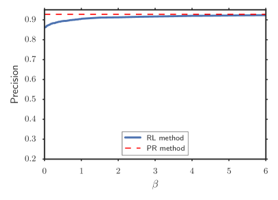
(a) RL Method vs PR method

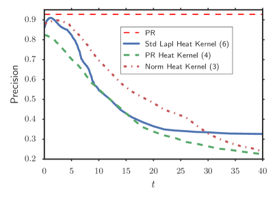
(b) Heat Kernel methods vs PR method

Figure 1: Les Miserables Dataset. Labelled points are chosen randomly.

To see better the behaviour of the heat kernel methods for large values of $t$, we have chosen a larger interval for $t$ in Figure 2. The performance of the heat kernel methods degrades quite significantly for large values of $t$. This is actually predicted by the asymptotics given in Section 5. Since we have more than two classes, the heat kernels with rank-one second order asymptotics are not able to distinguish among the classes. All heat kernel methods as well as the Regularized Laplacian method show a deterioration in performance for small values of $t$ and $\beta$. This was predicted in Section 5, as all the methods start to behave like the nearest neighbour method. In particular, as follows from the asymptotics of Section 5 and can be observed in the figures the Standard Laplacian heat kernel method and the Regularized Laplacian method shows exactly the same performance when $t\to 0$ and $\beta\to 0$.

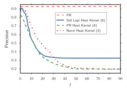
Figure 2: Les Miserables Dataset. Heat Kernel methods vs PR method, larger $t$.

It was observed in [5] that taking labelled data points with large (weighted) degree is typically beneficial for the semi-supervised learning methods. Thus, we now label randomly two points out of three points with maximal degree for each class. The average precision is given in Figure 3.(a). We also test heat kernel based methods with the same labelled points, see Figure 3.(b). One can see that if we choose the labelled points with large degree, the Regularized Laplacian Method outperforms the PageRank based method. Some heat kernel based methods with large degree labelled points also outperform the PageRank based method but their performance is much less stable with respect to the value of parameter $t$.

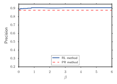
(a) RL Method vs PR method

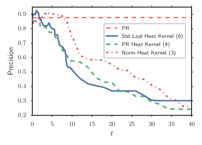
(b) Heat Kernel methods vs PR method

Figure 3: Les Miserables Dataset. Labelled points are chosen with large degrees.

Next, we consider the second dataset consisting of Wikipedia mathematical articles. This dataset is derived from the English language Wikipedia snapshot (dump) from January 30, 2010. The similarity graph is constructed by a slight modification of the hyper-text graph. Each Wikipedia article typically contains links to other Wikipedia articles which are used to explain specific terms and concepts. Thus, Wikipedia forms a graph whose nodes represent articles and whose edges represent hyper-text inter-article links. The links to special pages (categories, portals, etc.) have been ignored. In the present experiment we did not use the information about the direction of links, so the similarity graph in our experiments is undirected. Then we have built a subgraph with mathematics related articles, a list of which was obtained from “List of mathematics articles” page from the same dump. In the present experiments we have chosen the following three mathematical classes: “Discrete mathematics” (DM), “Mathematical analysis” (MA), “Applied mathematics” (AM). With the help of AMS MSC Classification and experts we have classified related Wikipedia mathematical articles into the three above mentioned classes. As a result, we obtained three imbalanced classes DM (106), MA (368) and AM (435). The subgraph induced by these three topics is connected and contains 909 articles. Then, the similarity matrix $A$ is just the adjacency matrix of this subgraph.

First, we have chosen uniformly at random 100 times 5 labeled nodes for each class. The average precisions corresponding to the Regularized Laplacian method and the PageRank based method are plotted in Figure 4.(a). We also provide the results for the three heat kernel based methods in Figure 4.(b). As one can see, the results of Wikipedia Mathematical articles dataset are consistent with the results of Les Miserables dataset.

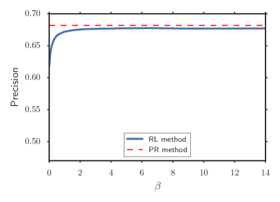
(a) RL Method vs PR method

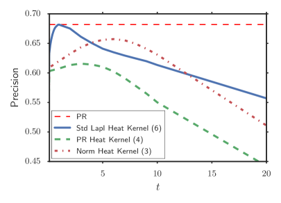
(b) Heat Kernel methods vs PR method

Figure 4: Wiki Math Dataset. Labelled points are chosen randomly.

Then, for each class out of 10 data points with largest degrees we choose 5 points and average the results. The average precisions for the Regularized Laplacian method, PageRank based method and for the three heat kernel based methods are plotted in Figure 5. The results are again consistent with the corresponding results for Les Miserables dataset. We would like to mention that for the computations in the Wiki Math dataset with many parameter settings and extensive averaging using NVIDIA CUDA sparse matrix library (cuSPARSE) [39] were noticeably faster than using numpy.linalg.solve calling LAPACK routine _gesv.

Finally, we would like to recall from Subsection 4.5 that a good value of $\beta$ can be provided by the ratio $\sigma_{1}^{2}/\sigma_{2}^{2}$, where $\sigma_{1}^{2}$ is the variance related to the data points and $\sigma_{2}^{2}$ is the variance related to the paired comparison between points. We can argue that $\sigma_{1}^{2}$ is naturally large and the paired comparisons between points can be performed with much more certainty, and hence, $\sigma_{2}^{2}$ is small. This gives a statistical explanation why it is good to take relatively large values for the parameter $\beta$ in the Regularized Laplacian method.

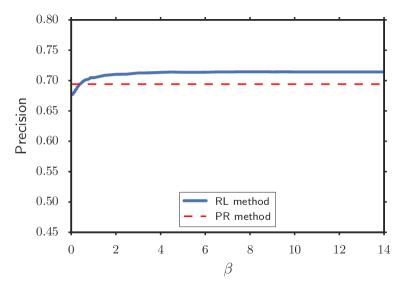
(a) RL Method vs PR method

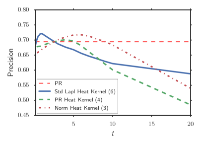
(b) Heat Kernel methods vs PR method

Figure 5: Wiki Math Dataset. Labelled points are chosen with large degree.

7 Conclusions

We have studied in detail the semi-supervised learning method based on the Regularized Laplacian. The method admits both linear algebraic and optimization formulations. The optimization formulation appears to be particularly well suited for parallel implementation. We have provided various interpretations and proximity-distance properties of the Regularized Laplacian graph kernel. We have also shown that the method is related to the Scheffé linear statistical model. The method was tested and compared with the other state of the art semi-supervised learning methods on two datasets. The results from the two datasets are consistent. In particular, we can conclude that the Regularized Laplacian method is comparable in performance with the PageRank based method and outperforms the related heat kernel based methods in terms of robustness.

Several interesting research directions remain open for investigation. It will be interesting to compare the Regularized Laplacian method with the other semi-supervised methods on a very large dataset. We are currently working in this direction. We observe that there is a large plateau of $\beta$ values for which the Regularized Laplacian method performs very well. It will be very useful to characterize this plateau analytically. Also, it will be interesting to understand analytically why the Regularized Laplacian method performs better when the labelled points with large degree are chosen.

References

- [1] Agaev, R. P. and Chebotarev, P. Y. (2001) “Spanning forests of a digraph and their applications”. Automation and Remote Control, 62(3), pp. 443–466.
- [2] Andersen, R., Chung, F., and Lang, K. (2006). “Local graph partitioning using pagerank vectors”. In Proceedings of IEEE FOCS 2006, pp. 475–486.
- [3] Avrachenkov, K., Dobrynin, V., Nemirovsky, D., Pham, S.K., and Smirnova, E. (2008). “Pagerank based clustering of hypertext document collections”. In Proceedings of ACM SIGIR 2008, pp. 873–874.
- [4] Avrachenkov, K., Gonçalves, P., Mishenin, A., and Sokol, M. (2012). “Generalized optimization framework for graph-based semi-supervised learning”. In Proceedings of SIAM Conference on Data Mining (SDM 2012) (Vol. 9).
- [5] Avrachenkov, K., Gonçalves, P., and Sokol, M. (2013). “On the choice of kernel and labelled data in semi-supervised learning methods”. In Algorithms and Models for the Web Graph, WAW 2013, also LNCS, Vol. 8305, pp. 56–67.
- [6] Avrachenkov, K., Mazalov, V. and Tsynguev, B. (2015) “Beta Current Flow Centrality for Weighted Networks”. In Proceedings of the 4th International Conference on Computational Social Networks (CSoNet 2015), also LNCS 9197, Chapter 19.
- [7] Blackwell, D. (1962). “Discrete dynamic programming”. The Annals of Mathematical Statistics, 33, pp. 719–726.
- [8] Callut, J., Françoisse, K., Saerens, M., and Dupont, P. (2008) “Semi-supervised classification from discriminative random walks”. In Machine Learning and Knowledge Discovery in Databases European Conference, ECML PKDD 2008, Antwerp, Belgium, September 15–19, 2008, Proceedings, Part I, ser. Lecture Notes in Computer Science / Lecture Notes on Artificial Intelligence, W. Daelemans, B. Goethals, and K. Morik, Eds., vol. 5211. Berlin-Heidelberg: Springer, pp. 162–177.
- [9] Chapelle, O., Schölkopf, B. and Zien A. (2006). Semi-supervised learning, MIT Press.
- [10] Chebotarev, P. Y. (1994). “Aggregation of preferences by the generalized row sum method”. Mathematical Social Sciences, 27, pp. 293–320.
- [11] Chebotarev, P. (2008). “Spanning forests and the golden ratio”. Discrete Applied Mathematics, 156(5), pp. 813–821.
- [12] P. Chebotarev (2011). “The graph bottleneck identity”. Advances in Applied Mathematics, 47(3), pp. 403–413.
- [13] Chebotarev, P. Yu., and Shamis, E. V. (1997). “The matrix-forest theorem and measuring relations in small social groups”. Automation and Remote Control, 58(9), pp. 1505–1514.
- [14] Chebotarev, P. Yu., and Shamis, E. V. (1998). “On a duality between metrics and -proximities”. Automation and Remote Control, 59(4), pp. 608–612.
- [15] Chebotarev, P. Yu., and Shamis, E. V. (1998). “On proximity measures for graph vertices”. Automation and Remote Control, 59(10), pp. 1443–1459.
- [16] Chebotarev, P. Yu., and Shamis, E. V. (2000). “The forest metrics of a graph and their properties”. Automation and Remote Control, 61(8), pp. 1364–1373.
- [17] Chung, F., and Yau, S. T. (1999). “Coverings, heat kernels and spanning trees”. Electronic Journal of Combinatorics, 6, R12.
- [18] Chung, F., and Yau, S. T. (2000). “Discrete Green’s functions”. Journal of Combinatorial Theory, Series A, 91(1), pp. 191–214.
- [19] Chung, F. (2007). “The heat kernel as the pagerank of a graph”. PNAS, 105(50), pp. 19735–19740.
- [20] Chung, F. (2009). “A local graph partitioning algorithm using heat kernel pagerank”. In Proceedings of WAW 2009, LNCS 5427, pp. 62–75.
- [21] Critchley, F. (1988) “On certain linear mappings between inner-product and squared-distance matrices”. Linear Algebra and its Applications, 105, pp. 91–107.
- [22] Deza, M. M., and Laurent, M. (1997) Geometry of Cuts and Metrics, volume 15 of Algorithms and Combinatorics. Berlin: Springer.
- [23] Fouss, F., Francoisse, K., Yen, L., Pirotte A., and Saerens, M. (2012) “An experimental investigation of kernels on graphs for collaborative recommendation and semisupervised classification”. Neural Networks, 31, pp. 53–72.
- [24] Dorugade, A. V. (2014) “New ridge parameters for ridge regression”. Journal of the Association of Arab Universities for Basic and Applied Sciences, 15, pp. 94–99.
- [25] Fouss, F., Yen, L., Pirotte, A., and Saerens, M. (2006) “An experimental investigation of graph kernels on a collaborative recommendation task”. In Sixth International Conference on Data Mining (ICDM’06), pp. 863–868.
- [26] Kirkland, S. J., Neumann, M., and Shader, B. L. (1997) “Distances in weighted trees and group inverse of Laplacian matrices”. SIAM J. Matrix Anal. Appl., 18, pp.827–841.
- [27] Knuth, D. E. (1993). The Stanford GraphBase: a platform for combinatorial computing. ACM, New York, NY, USA.
- [28] Kondor, R. I., and Lafferty, J. (2002). “Diffusion kernels on graphs and other discrete input spaces”. In Proceedings of ICML, 2, pp. 315–322.
- [29] Muniz, G. and Kibria, B. M. G. (2009) “On some ridge regression estimators: An empirical comparisons”. Communications in Statistics – Simulation and Computation, 38(3), pp. 621–630.
- [30] Newman, M. E. J. and Girvan, M. (2004). “Finding and evaluating community structure in networks”. Phys. Rev. E, 69(2):026113.
- [31] Puterman, M. L. (1994). Markov decision processes: Discrete stochastic dynamic programming, John Wiley & Sons.
- [32] Scheffé, H. (1952) “An analysis of variance for paired comparisons”. Journal of the American Statistical Association, 47(259), pp. 381-400.
- [33] Smola, A. J., and Kondor, R. I. (2003) “Kernels and regularization of graphs”. In Proceedings of the 16th Annual Conference on Learning Theory, pp. 144–158.
- [34] Yen, L., Saerens, M., Mantrach, A., and Shimbo, M. (2008) “A family of dissimilarity measures between nodes generalizing both the shortest-path and the commutetime distances”. In 14th ACM SIGKDD Intern. Conf. on Knowledge Discovery and Data Mining, pp. 785–793.
- [35] Zhou, D., and Burges, C. J. C. (2007) “Spectral clustering and transductive learning with multiple views”. In Proceedings of ICML 2007, pp. 1159–1166.
- [36] Zhou, D., Bousquet, O., Navin Lal, T., Weston, J., Schölkopf, B. (2004). “Learning with local and global consistency”. In: Advances in Neural Information Processing Systems, 16, pp. 321–328.
- [37] Zhu, X., Ghahramani, Z., and Lafferty, J. (2003). “Semi-supervised learning using Gaussian fields and harmonic functions”. In Proceedings of ICML 2003, Vol. 3, pp. 912–919.
- [38] Zhu, X. (2005). “Semi-supervised learning literature survey”. University of Wisconsin-Madison Research Report TR 1530.
- [39] The NVIDIA CUDA Sparse Matrix library (cuSPARSE), https://developer.nvidia.com/cuSPARSE