Tolerating Correlated Failures in Massively Parallel Stream Processing Engines

Abstract

Fault-tolerance techniques for stream processing engines can be categorized into passive and active approaches. A typical passive approach periodically checkpoints a processing task’s runtime states and can recover a failed task by restoring its runtime state using its latest checkpoint. On the other hand, an active approach usually employs backup nodes to run replicated tasks. Upon failure, the active replica can take over the processing of the failed task with minimal latency. However, both approaches have their own inadequacies in Massively Parallel Stream Processing Engines (MPSPE). The passive approach incurs a long recovery latency especially when a number of correlated nodes fail simultaneously, while the active approach requires extra replication resources. In this paper, we propose a new fault-tolerance framework, which is Passive and Partially Active (PPA). In a PPA scheme, the passive approach is applied to all tasks while only a selected set of tasks will be actively replicated. The number of actively replicated tasks depends on the available resources. If tasks without active replicas fail, tentative outputs will be generated before the completion of the recovery process. We also propose effective and efficient algorithms to optimize a partially active replication plan to maximize the quality of tentative outputs. We implemented PPA on top of Storm, an open-source MPSPE and conducted extensive experiments using both real and synthetic datasets to verify the effectiveness of our approach.

I Introduction

There is a recently emerging interest in building Massively Parallel Stream Processing Engines (MPSPE), such as Storm [24], and Spark Streaming[26], which make use of large-scale computing clusters to process continuous queries over fast data streams. Such continuous queries often run for a very long time and would unavoidably experience various system failures, especially in a large-scale cluster. As it is critical to provide continuous query results without significant downtime in many data stream applications, fault-tolerance techniques in Stream Processing Engines (SPEs) [3, 5, 26] have attracted a lot of attention.

Existing fault-tolerance techniques for SPEs can be generally categorized as passive and active approaches [13]. In a typical passive approach, the runtime states of tasks will be periodically extracted as checkpoints and stored at different locations. Upon failure, the state of a failed task can be restored from its latest checkpoint. While one can in general tune the checkpoint frequency to achieve trade-offs between the cost of checkpoint and the recovery latency, the checkpoint frequency should be limited to avoid high checkpoint overhead, which affects the system performance. Hence recovery latency is usually significant in a passive approach. When one wants to minimize the recovery latency as much as possible, it is often more efficient to use an active approach, which typically uses one backup node to replicate the tasks running on each processing node. When a node fails, its backup node can quickly take over with minimal latency.

Even though there are abundant fault-tolerance techniques in SPEs, developing an MPSPE [24] poses great challenges to the problem. First of all, in a large cluster, there are often two different types of failures: independent failure and correlated failure [10, 21]. Previous studies mostly focused on independent failure that happens at a single node. Correlated failures are usually caused by failures of switches, routers and power facilities, and will involve a number of nodes failing simultaneously. With such failures, one has to recover a large number of failed tasks and temporarily run them on an additional set of standby nodes before the failed ones are recovered. Using a passive fault tolerance approach, one has to keep the standby nodes running even their utilization is low most of the time in order to avoid the unacceptable overhead of starting them at recovery time. Furthermore, as checkpoints of different nodes are often created asynchronously, massive synchronizations have to be performed during recovery. Therefore it could be difficult to meet the user requirements on recovery latency even with a relatively high checkpoint frequency.

On the other hand, while an active fault-tolerance approach can achieve a lower recovery latency, it could be too costly for a large-scale computation. Consider a large-scale stream computation that is parallelized onto $100$ nodes, one may not be able to afford another $100$ backup nodes for active replication.

Another challenge is that there exist some time-critical applications which prefer query outputs being generated in good time even if the outputs are computed based on incomplete inputs. This kind of applications usually require continuous query output for real-time opportune decision-making or visualization. Consider a community-based navigation service, which collects and aggregates user-contributed traffic data in a real-time fashion and then continuously provides navigation suggestions to the users. Failure of some processing nodes could result in losing some user-contributed data. The system, while waiting for the failed nodes to recover, can continue to help drivers plan their routes based on the incomplete inputs. Other examples of such applications are like intrusion detections, online visualization of real-time data streams etc. Alerts of events matching the intrusion attack patterns or infographics generated over incomplete inputs are still meaningful to the users and should be generated without any major delay. Consider the long recovery latency for a large-scale correlated failure, the lack of trade-offs between recovery latency and result quality would not be able to fulfill the requirements of these applications.

To address the aforementioned challenges, we propose a new fault-tolerance scheme for MPSPEs, which is Passive and Partially Active (PPA). In a PPA scheme, a number of standby nodes will be used to prepare for recoveries from both independent and correlated failures. Checkpoints of the processing nodes will be stored at the standby nodes periodically. Rather than keeping them mostly idled as in a purely passive approach, we opportunistically employ them for active replications for a selected subset of the running tasks. In this way, we can provide very fast recovery for the tasks with active replicas. Furthermore, when the failed tasks contain those without active replicas, PPA provides tentative outputs with quality as high as possible. The results can then be rectified after the passive recovery process has been finished using similar techniques proposed in [3]. In general, PPA is more flexible in utilizing the available resources than a purely active approach, and in the meantime can provide tentative outputs with a higher quality than a purely passive one.

In this paper, we focus on optimizing utilizing available resources for active replication in PPA, i.e. deciding which tasks should be included for active replication. In summary, we have made the following contributions in this paper:

(1) We present PPA, a passive but partially active fault-tolerance scheme for a MPSPE.

(2) As existing MPSPEs often involve user defined functions whose semantics are not easily available to the system, we propose a simple yet effective metric, referred to as output fidelity, to estimate the quality of the tentative outputs.

(3) We propose an optimal dynamic programming algorithms and several heuristic algorithms to determine which tasks to actively replicate for a given query topology.

(4) We implement our approach in an open-source MPSPE, namely Storm [24] and perform an extensive experimental study on an Amazon EC2 cluster using both real and synthetic datasets. The results suggest that by adopting PPA, the accuracy of tentative outputs are significantly improved with limited amount of replication resources.

II System Model

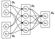
Figure 1: A topology that consists of $4$ operators ($O_{1},O_{2},O_{3},O_{4}$) with different numbers of tasks.

II-A Data and Query Model

As in existing MPSPEs [24], we assume that a data item is modeled as a key-value pair. Without loss of generality, the key of a data item is assumed to be a string and the value is a blob in an arbitrary form that is opaque to the system.

A query execution plan in MPSPEs typically consists of multiple operators, each being parallelized onto multiple processing nodes based on the key of input data. Each operator is assumed to be a user-defined function. We model such query plan as a topology of the parallel tasks of all the query operators. By modeling each task as a vertex and the data flow between each pair of tasks as a directed edge, the query topology can be represented as a Directed Acyclic Graph (DAG). Figure 1 shows an example query topology. Each task represents the workload of an operator that is assigned to a processing node in the cluster and all the tasks that belong to the same operator will conduct the same computation.

An operator can subscribe to the outputs from multiple operators except for itself. The output stream of every task will be partitioned into a set of substreams using a particular partitioning function, which divides the keys of a stream into multiple key partitions and splits the stream into substreams based on these key partitions. For each task, the input substreams received from the tasks belonging to the same upstream neighboring operator will constitute an input stream. Therefore, the number of input streams of a task is up to the number of its upstream neighboring operators.

Similar to [28], we consider the following four common partitioning situations between two neighboring operators in a MPSPE. In the following descriptions, we consider an upstream operator containing $N_{1}$ tasks and a downstream operator containing $N_{2}$ tasks.

• One-to-one: each upstream task only sends data to a single downstream task and a downstream task only receives data from a single upstream task.

• Split: each upstream task sends data to $M_{2}$, $2\leq M_{2}<N_{2}$, downstream tasks and each downstream task only receives data from a single upstream task.

• Merge: each upstream task sends data to only one downstream task and each downstream task receives data from $M_{1}$, $2\leq M_{1}<N_{1}$, upstream tasks.

• Full: each upstream task sends data to all $N_{2}$ downstream tasks.

II-B PPA Replication Plan

Given a topology $T$ and its whole set of tasks $\mathcal{M}$, a PPA replication plan for $T$ consists of two parts: a passive replication plan that covers all the tasks in $\mathcal{M}$ and a partially active replication plan which covers a subset of $\mathcal{M}$, denoted as $\mathbf{P}$. With the passive replication plan, checkpoints will be periodically created for all the tasks and stored at the standby nodes. For a task $t_{i}$, its checkpoint consists of $t_{i}$’s computation state and output buffer. After a checkpoint is extracted from $t_{i}$, its upstream neighboring tasks will be notified to prune the unnecessary data from their output buffers. The buffer trimming should guarantee that, if $t_{i}$ fails, its computation state can be recovered by loading its latest checkpoint and replaying the output buffers in its upstream tasks. On the other hand, for each $t_{i}\in\mathbf{P}$, an active replica will be created, which will receive the same input data and perform the same processing as $t_{i}$’s primary copy.

Upon failures, the actively replicated tasks will be recovered immediately using their active replicas, meanwhile the tasks that are only passively replicated will be restored from their latest checkpoints. When there are some failed tasks belonging to $\mathcal{M}-\mathbf{P}$, tentative outputs will be produced before they are fully recovered. Such tentative outputs have a degraded quality due to the loss of input data that otherwise should be processed by the failed tasks belonging to $\mathcal{M}-\mathbf{P}$. We present how to optimize the partially active replication plan to maximize the quality of tentative outputs and the details of the system implementation in the following sections.

III Problem Formulation

III-A Quality of Tentative Outputs

Previous works on load shedding [2, 16] have studied how to evaluate the quality of query outputs in case of lost of input data. Their models assume full knowledge of the semantics of individual operators and hence can estimate the output quality in a relatively precise way. However, in existing MPSPEs, such as Storm, operators are often opaque to the system and may contain complex user-defined functions written in imperative programming languages. The existing models therefore cannot be easily applied. In our first attempt, we have tried to derive output accuracy models composed by some generic functions, which should be chosen or provided by the users according to the semantics of the operators. We found that this approach is not very user friendly and it may be very difficult for a user to provide such functions for a complicated operator.

Therefore, we strive to design a model that requires users to provide minimum information of an operator’s semantic, but yet is effective in estimating the quality of tentative outputs. More specifically, we propose a metric, called Output Fidelity $\left(OF\right)$, which is roughly equal to the ratio of the source input that can contribute to tentative outputs. This is based on the assumption that the accuracy of tentative outputs increases with more complete input and a PPA plan with a higher OF value would incur more accurate tentative outputs.

III-A1 Operator Output Loss Model

It is the sink operator that produces the final outputs of a topology. As task failures can happen at any position within the topology, we need to propagate the information losses incurred by any failed task to the output of the sink operator. Suppose task $t_{22}$ in Figure 2 is failed, we need to transform the input loss of $t_{31}$ into its output loss. In this subsection, we propose the operator output loss model, which estimates the information loss of an operator’s output based on the information loss of its input. In the next subsection, we present the precise definition of OF.

In following descriptions, the set of input streams of task $t_{i}$ are denoted as $\left\{S_{i,1}^{in},S_{i,2}^{in},...,S_{i,p}^{in}\right\}$, where the rate of $S_{i,j}^{in}$ is represented as $\lambda_{i,j}^{in}$ and its information loss is referred to as $IL_{i,j}^{in}$. The rate of $t_{i}$’s output stream, $S_{i}^{out}$, is referred to as $\lambda_{i}^{out}$, and its information loss is denoted as $IL_{i}^{out}$. If $t_{i}$ is failed, its output will be lost and $IL_{i}^{out}$ will be set as $1$. Otherwise, we calculate $IL_{i}^{out}$ based on the information losses of $t_{i}$’s input streams.

As described in the query model, an input stream of a task may consist of multiple substreams, which are sourced from tasks belonging to the same upstream neighboring operator. Suppose that $S_{i,j}^{in}$ consists of a set of substreams $U_{i,j}^{in}$. For each substream $s_{k}$, $s_{k}\in U_{i,j}^{in}$, denoting its rate as $\lambda_{s_{k}}$ and its information loss as $IL_{s_{k}}$, then the information loss of $S_{i,j}^{in}$ is calculated as:

$$IL_{i,j}^{in}=\frac{\sum_{s_{k}}^{s_{k}\in U_{i,j}^{in}}\lambda_{s_{k}}\cdot IL_{s_{k}}}{\sum_{s_{k}}^{s_{k}\in U_{i,j}^{in}}\lambda_{s_{k}}}$$ (1)

Meanwhile, the output stream of task $t_{i}$, $S_{i}^{out}$, can be split into a set of substreams, denoted as $D_{i}^{out}$. For each substream $s_{k}$ belonging to $D_{i}^{out}$, its information loss is estimated to be equal to $S_{i}^{out}$, i.e. $IL_{s_{k}}=IL_{i}^{out}$.

Figure 2 depicts an example topology as well as the rate of each output stream. $IL_{31}^{out}$ represents the information loss of output stream $S_{31}^{out}$ caused by the failure of task $t_{22}$. We distinguish two situations and use this example to illustrate the calculation of information loss of a task’s output stream.

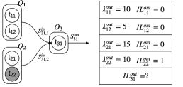
Figure 2: An illustrating topology with task failure, where $\lambda_{31,1}^{in}=\lambda_{11}^{out}+\lambda_{12}^{out}$ and $\lambda_{31,2}^{in}=\lambda_{21}^{out}+\lambda_{22}^{out}$.

Correlated-Input Operator. $O_{t}$ performs computations over the join results of its input streams. For example, suppose $O_{3}$ in Figure 2 is a join operator. Without further semantic information of $O_{3}$, we consider the effective input of $t_{31}$ as the Cartesian product of its input streams, whose rate is equal to $\left(\lambda_{31,1}^{in}\cdot\lambda_{31,2}^{in}\right)$ and its information loss can be computed as $\left[1-\left(1-IL_{31,1}^{in}\right)\cdot\left(1-IL_{31,2}^{in}\right)\right]$. By assuming that the information loss of $t_{31}$’s output should be equal to that of its input stream, we can get $IL_{31}^{out}=\frac{2}{5}$. In summary, the information loss of $t_{i}$’s output stream can be calculated as:

$$IL_{i}^{out}=1-\prod_{j=1}^{p}\left(1-IL_{i,j}^{in}\right)$$ (2)

Independent-Input Operator. $O_{t}$ does not compute joins over input streams. If $O_{3}$ in Figure 2 is an independent-input operator, the effective input of $t_{31}$ is considered as the union of its input streams, whose rate is equal to $\left(\lambda_{31,1}^{in}+\lambda_{31,2}^{in}\right)$ and its input loss can be calculated as $\frac{\lambda_{31,1}^{in}\cdot IL_{31,1}^{in}+\lambda_{31,2}^{in}\cdot IL_{31,2}^{in}}{\lambda_{31,1}^{in}+\lambda_{31,2}^{in}}$. Similar to the correlated-input operator, we also assume that the information loss of $t_{31}$’s ouptut should be equal to that of its input stream. Then we have, in this example, $IL_{31}^{out}=\frac{1}{4}$. In general, the information loss of $t_{i}$’s output stream can be calculated as follows:

$$IL_{i}^{out}=\frac{\sum_{j=1}^{p}\lambda_{i,p}^{in}\cdot IL_{i,p}^{in}}{\sum_{k=1}^{p}\lambda_{i,k}^{in}}$$ (3)

Recall that one of the design principles is to request as little information of the operators’ semantics as possible. We distinguish the aforementioned two types of operators simply because the characteristics of their effective inputs are very different. With such distinction, the OF metric can be estimated much more precisely.

III-A2 Output Fidelity

With the operator output loss model, the output information losses of tasks in the sink operator can be calculated by conducting a depth-first traversal of the topology, which starts from the tasks in the source operators and ends at the tasks in the sink operator.

By denoting the sink operator of topology $T$ as $O_{sink}$, and the set of tasks belonging to $O_{sink}$ as $\left\{t_{1},t_{2},...,t_{M_{t}}\right\}$, The output fidelity of topology $T$, $OF_{T}$, is defined as:

$$OF_{T}=1-\frac{\sum_{i=1}^{M_{t}}\lambda_{i}^{out}\cdot IL_{i}^{out}}{\sum_{j=1}^{M_{t}}\lambda_{j}^{out}}$$ (4)

III-B Problem Statement

Before presenting the problem definition, we introduce a concept: Minimal Complete Tree, which is also referred to as MC-tree for simplicity in the following sections.

Definition 1.

Minimal Complete Tree (MC-Tree): A minimal complete tree is a tree-structured subgraph of the topology DAG. The source vertices of this subgraph correspond to tasks from the source operators and its sink vertex is a task from an output operator. A minimal complete tree can continuously contribute to final outputs if and only if all its tasks are alive.

Taking the topology in Figure 1 for instance, if $O_{3}$ is an independent-input operator, tasks in $\left\{t_{11},t_{31},t_{41}\right\}$ can constitute an MC-tree and there are in total $16$ MC-trees in the topology. However, if $O_{3}$ is a correlated-input operator, $t_{31}$ cannot produce any output if either $t_{11}$ or $t_{21}$ fails. Hence tasks in $\left\{t_{11},t_{21},t_{31},t_{41}\right\}$ can constitute an MC-tree and the number of MC-trees in the topology is equal to $8$.

Based on Definition 1, if failures of tasks in an MC-Tree occur, it will only continue propagating data to the sink operator if and only if all of its failed tasks are actively replicated. Suppose topology $T$ consists of a set of operators $O_{1},O_{2},...,O_{N}$ and the available resources can be used to actively replicate $R$ tasks ($R\leq|\mathcal{M}|$, where $\mathcal{M}$ is all the tasks of $T$), then the problem of optimizing a partially active replication plan is defined as follows:

Definition 2.

Partially Active Plan: Given a query topology $T$, choose $R$ tasks for active replication such that, the output fidelity of the partial topology that is composed of the actively replicated MC-trees in $T$ is maximized.

This problem is NP-hard, as it can be polinomially reduced from the Set-Union Knapsack Problem [8], which is NP-hard.

IV Active Replication Optimization

Recall that we consider the worst case scenario for a correlated failure, i.e. there is at least one failed task in every MC-tree. Before the completion of the passive recovery process, only the MC-trees whose failed tasks are actively replicated can produce tentative outputs. The optimization objective is to maximize the value of OF with limited amount of resources used for active replication.

IV-A Dynamic Programming

We first present a dynamic programming algorithm that can generate an optimal replication plan for correlated failure. As has been introduced in section III-B, we take MC-tree as the basic unit for replication candidates in the algorithm.

Input: Amount of available resources $R$;

Output: Replication plan $\mathbf{P}$;

1 $CP_{0}\leftarrow\emptyset$; $usage\leftarrow 0$; $SC\leftarrow\{CP_{0}\}$;

/* $CP_{0}$:initial replication plan; $SC$:candidate plan set; */

2

3while $usage++<R$ do

4       foreach candidate plan $CP_{i}$ in $SC$ do

5             $dif\leftarrow usage-|CP_{i}|$;

             /* $|CP_{i}|$ is the number of replicated tasks in $CP_{i}$ and $dif$ is the number of tasks that can be added to $CP_{i}$ at this step; */

6             $UT_{i}\leftarrow\{$ MC-tree $tr\mid tr\notin CP_{i}\}$;

7             $u_{i}\leftarrow$ $\max\{\mathbf{nonrep\_tasks}(tr,CP_{i})\mid tr\in UT_{i}\}$;

             /* $\mathbf{nonrep\_tasks}(tr,CP_{i})$ returns the number of non-replicated tasks of MC-tree $tr$ in $CP_{i}$; */

8             if $dif\leq u_{i}$ then

9                   foreach $\textrm{MC-tree }tr_{j}\in\{tr\mid tr\notin CP_{i}~{}\&~{}\mathbf{nonrep\_tasks}(tr_{j},CP_{i})==dif\}$ do

10                         $CP_{j}\leftarrow CP_{i}\cup tr_{j}$;

11                         if $CP_{j}\notin SC$ then

12                               Add $CP_{j}$ to $SC$;

13                              

14            else Remove $CP_{i}$ from $SC$;

15            ;

16            

$\mathbf{P}\leftarrow$ the candidate plan in $SC$ with the maximal OF value. Return $\mathbf{P}$;

Algorithm 1 Dynamic Programming: PlanCorrelatedFailure($R$)

Details of this algorithm are presented in Algorithm 1. It is essentially a bottom-up dynamic programming algorithm. We incrementally increase the number of resources to be used for active replication and enumerate the possible expansions of the plans produced in the previous step. Assuming the minimum size of MC-trees is $r$, one can obtain the first set of replication plans, referred to as $SC$, by replicating $r$ tasks. At this step, each plan in $SC$ contains exactly one MC-tree. Note that the MC-trees that have not been added to a candidate plan $CP_{i}$ may also have replicated tasks if they share some tasks with another MC-tree within $CP_{i}$.

At the next iteration of the while loop starting at line $2$, we increase the resource usage by $1$. We scan through each candidate plan $CP_{i}\in SC$ to see if there is an MC-tree $tr_{j}\notin CP_{i}$ that contains a number of non-replicated tasks which is equal to $usage-|CP_{i}|$, where $|CP_{i}|$ is the number of replicated tasks in $CP_{i}$. For each MC-tree satisfying this condition, we create a new candidate plan $CP_{j}$ (line $9$) such that $CP_{j}\leftarrow CP_{i}\cup tr_{j}$. If $CP_{j}$ has no duplicate in $SC$, then it will be inserted into $SC$. The algorithm will continue until $usage$ is equal to the limit $R$.

The cost of scanning through $SC$ can be reduced by removing a candidate plan $CP_{i}$ from $SC$ if all its possible expansions have been considered. More precisely, remove $CP_{i}$ from $SC$ if the maximum number of non-replicated tasks of the MC-trees not included in $CP_{i}$ is less than the difference between the available resource at the current iteration, i.e. $usage$, and the current number of replicated tasks in $CP_{i}$ (lines $7$ and $12$). After the while loop is finished, the candidate plan with the maximal OF in $SC$ will be returned.

The upper bound of the complexity of this algorithm is $O\left(2^{\mathcal{T}}\right)$, where $\mathcal{T}$ is the number of MC-trees in the query topology, which varies with the topology structures and has an upper bound of $O(M^{N})$, where $N$ is the number of operators and $M$ is the average degree of parallelization of operators in $T$. The following theorem states the optimality of this dynamic programing algorithm, the proof is skipped due to space limitation.

Theorem 1.

Let $\mathbf{P}$ be the replication plan produced by Algorithm 1 and $\mathbf{P_{t}}$ be a different replication plan. If $OF_{P_{t}}\geq OF_{P}$, then the resource usage of $\mathbf{P}$ is always equal to or less than that of $\mathbf{P_{t}}$.

1

Input: The amount of available resources $R$;

Output: Replication plan $\mathbf{P}$

2 Initialize: $AS\leftarrow\emptyset$;

3 foreach Task $t_{i}\notin\mathbf{P}$ do

4       $A_{i}\leftarrow$ the value of OF if only $t_{i}$ fails;

5       $AS\leftarrow AS\cup\{A_{i}\}$;

6      

7Sort $AS$ in ascending order;

8 $TS\leftarrow$ set of tasks whose corresponding OF values are among top-$R$ in $AS$;

9 $\mathbf{P}\leftarrow\mathbf{P}\cup TS$;

Return $\mathbf{P}$

Algorithm 2 Greedy($R$)

IV-B Greedy Algorithm

We present a greedy algorithm. For each task in the topology, the greedy algorithm will calculate the OF of the topology by only failing this task. A task whose failure would lead to a smaller OF will be assigned a higher priority for replication. We present the details of this greedy algorithm in Algorithm 2, which will first rank all the tasks in ascending order based on the OF calculated by their respective failures. Then it will iterate to choose the corresponding task that would cause the minimal OF among all the remaining non-replicated tasks in the set $AS$.

The complexity of the greedy algorithm is $O(N\cdot M)$, where the notations are defined in Section IV-A. Although this complexity is much lower than that of the dynamic programming algorithm, it fails to consider whether the tasks in the replication plan could form complete MC-trees, which will damage its performance especially when the number of active replicated tasks is small. The experimental results in section VI-B can verify this defect of the greedy algorithm.

IV-C Structure-Aware Algorithm

The dynamic programming algorithm searches for the optimal plan by selecting a subset of MC-trees for replication under the resource constraint to maximize the value of OF. Inspired by this, we design a structure-aware algorithm that, at each step, rather than enumerating all the possible expansions of a candidate plan, only expands it with an MC-tree that can incur the greatest increase in OF per resource unit.

Unfortunately, even such a greedy approach may fall short under the following situation. Consider a topology $T$ that consists of a sequence of $k$ operators and all the operators use Full partitioning, the number of MC-trees within $T$ is equal to $\prod_{i=1}^{k}M_{i}$, where $M_{i}$ is the number of tasks of operator $O_{i}$. In such a topology, the number of MC-trees will grow very fast with increasing number of operators. Therefore, even a greedy search among the possible combinations of MC-trees would not perform well.

To solve this problem, we firstly decompose a general topology into two types of topologies, namely full topologies and structured topologies, and then optimize them separately. The definitions of these two types of topologies are as follows:

• Structured topology is defined as a topology where only the operators, that produce outputs of this topology, can have a Full partitioning function and the others have other types of partitioning functions.

• Full topology is defined as a topology that all of its operators have a Full partitioning function.

The rest of this section is organized as follows: firstly, we present the algorithms generating PPA plans for structured topologies and full topologies respectively. Then we will explain the structure-aware algorithm, which generates the PPA plan for a general topology by decomposing it into several sub-topologies, each being either a structured topology or a full topology.

IV-C1 Algorithm for Structured Topology

Input: An initial plan $\mathbf{P}$; The amount of available resources $R$; Topology $T$;

1

Output: Replication plan $\mathbf{P}$;

2

3$usage=0$; $S_{u}\leftarrow$ Set of the units split from topology $T$;

4

5foreach Unit $U_{i}\in S_{u}$ do

6       Build segment set $G_{i}$;

7      

8while $usage\leq R$ do

9       $Candidates\leftarrow\emptyset$ ;

10       foreach Unit $U_{i}\in S_{u}$ do

11             foreach non-replicated segment $g_{i}\in U_{i}$ do

12                   $CG_{i}\leftarrow\{g_{i}\}$;

13                   if ${OF_{\mathbf{P}}}={OF_{\mathbf{P}\cup CG_{i}}}$  then

14                         Conduct a BFS from $U_{i}$ to traverse all the units:

15                         foreach visited unit $U_{j}$ during the BFS do

16                               Segment $g_{j}\leftarrow\mathbf{max\_of}\left(U_{j}\right)$ ;

                               /* $\mathbf{max\_of}\left(U_{j}\right)$ returns the segment in $U_{j}$, which is connected with segment in $CG_{i}$ and has the maximal OF with $U_{j}$ treated as an independent topology; */

17                               if $|CG_{i}|+|g_{j}|\leq usage$ then

18                                    $CG_{i}=CG_{i}\cup g_{j}$;

19                              else Stop the BFS;

20                               ;

21                              

22                  $Candidates\leftarrow Candidates\cup CG_{i}$;

23                  

24      Find $CG_{opt}$ from $Candidates$ such that the following value is maximized: $({OF_{\mathbf{P}\cup CG_{opt}}-OF_{\mathbf{P}}})/{|CG_{opt}|}$;

25       $\mathbf{P}=\mathbf{P}\cap CG_{opt}$; $usage=usage+|CG_{opt}|$;

26      

27      if $CG_{opt}\neq\emptyset$ then return $\mathbf{P}$;

28      ;

29      

30      Remove the completely replicated units from $S_{u}$;

31Return $\mathbf{P}$;

Algorithm 3 PlanStructuredTopology($\mathbf{P},R,T$)

Although we define structured topology such that Full partitioning only exists in the output operators, the number of MC-trees in a structured topology could still be very large. Consider the situation that a task $t_{i}$ receives $N_{in}$ input streams and produce $N_{out}$ output streams, there will be at least $N_{in}*N_{out}$ MC-trees containing $t_{i}$. In addition, if $t_{i}$ joins $N_{k}$ substreams from operator $O_{k}$ with $N_{j}$ substreams from operator $O_{j}$, the number of MC-trees containing $t_{i}$ will at least be equal to $N_{k}\cdot N_{j}$. To avoid bad performance due to the large number of MC-trees, we split a structured topology into multiple units such that, within a unit, the number of MC-trees is equal to the maximal number of input substreams among the operators of this unit. We refer to an MC-tree in a unit as segment to differentiate it from the concept of a complete MC-tree in the topology.

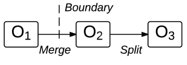
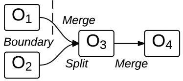
Figure 3: Examples of splitting structured topologies into units. $O_{3}$ in Figure 3 is a join operator.

The situation of multiple input streams and multiple output streams occurs on the task who has an input stream partitioned with Merge and an output stream partitioned with Split, a unit boundary will be set between this operator and its upstream neighboring operator using Merge partitioning. For instance, a unit boundary is set between $O_{1}$ and $O_{2}$ in the topology in Figure 3. The situation that a task joins multiple input substreams from one operator with substreams from other operators happens on the tasks of join operators that have at least one input stream partitioned with Merge. As illustrated in Figure 3, a unit boundary is set between $O_{1}$ and $O_{3}$.

Note that, with such a decomposed topology, replicating a segment is beneficial only if all the other segments within the same complete MC-tree are also replicated. In other words, we should avoid enumerating plans that replicate a set of disconnected segments.

The details of the algorithm for structured topology are presented in Algorithm 3. The algorithm searches through the units generated from input topology. Within unit $U_{i}$, if the set of non-replicated segments is not empty, we check whether replicating these segments will increase the final output accuracy (line $9$). Note that this will only be true if this segment can form a complete MC-tree with the other replicated segments within the current plan. Each of such segments will be put into a candidate pool (line $16$). If the segment $g_{i}$ does not enhance the plan’s OF, we conduct a BFS (Breadth-first search) starting from $U_{i}$ and traversing through all the units in Topology T. The BFS is terminated until $usage$ is less then the non-replicated tasks in $CG_{i}$. Finally, every unit visited during the BFS contributes a segment to $CG_{i}$ and the segments from neighboring units are connected (lines $10-15$). Then we put such a set of segments as one candidate in the candidate pool.

After finishing the scanning of all units, we get a candidate pool consisting of a number of segment sets, each containing one or more segments. We use a profit density function to rank the candidates. The profit density of a candidate $CG_{k}$ is calculated as $\left.\left(OF_{P\cup CG_{k}}-OF_{P}\right)\middle/|CG_{k}|\right.$, where $OF_{P}$ is the OF value of plan $P$, $OF_{P\cup CG_{k}}$ is the OF value after expanding $P$ by replicating segment in $CG_{k}$. $|CG_{K}|$ is the number of non-replicated tasks within $CG_{k}$. The plan in the candidate pool with the maximum profit density will be merged with the input plan $P$ and returned. The complexity of Algorithm 3 is equal to $O(R\cdot N\cdot M^{2}\cdot E)$, where $R$ is the amount of available replication resources, $N$ is the number of operators, $M$ represents the average degree of parallelization of operators in $T$, and $E$ is the number of neighboring unit pairs.

Input: Initial replication plan $\mathbf{P}$; Amount of available resources $R$; Topology $T$;

Output: Replication Plan $\mathbf{P}$

1 Initialize: $usage\leftarrow 0$;

2 $N\leftarrow\;Number\;of\;operators$;

3 Sort the set of tasks $S_{i}$ of each operator $O_{i}$ based on the OF increase, $\delta_{ij}$ , of tasks;

4 if $P=\emptyset\;\&\;N\leq R$ then

5       foreach $O_{i}$ do

6             Let $p_{ik}$ be the node in $S_{i}$ that has the largest OF increase $\delta_{ik}$;

7             $\mathbf{P}\leftarrow\mathbf{P}\cup\{p_{ik}\}$; $S_{i}\leftarrow S_{i}-\{p_{ik}\}$;

8            

9      $usage=N$;

10      

11if $\mathbf{P}=\emptyset\;\&\;N>R$ then return $\mathbf{P}$;

12;

13 while $usage<R$ do

14       $Candidates\leftarrow\emptyset$;

15       foreach $O_{i}$ do

16             Let $p_{ik}$ be the node in $S_{i}$ that has the largest OF increase $\delta_{ik}$;

17             $Candidates\leftarrow Candidates\cup P_{i}\cup\{p_{ik}\}$;

18            

19      $P_{j}\leftarrow\mathrm{\mathbf{max\_accuracy\_plan}}(Candidates)$;

20       $S_{j}\leftarrow S_{j}-\{p_{jk}\}$; $\mathbf{P}\leftarrow P_{j}$; $usage++$;

21      

22Return $\mathbf{P}$;

Algorithm 4 PlanFullTopology($\mathbf{P}$, $R$, $T$)

IV-C2 Algorithm for Full Topology

Each task within a full topology will send input data to all the tasks that belong to its downstream neighboring operators. We propose an algorithm for full topology as illustrated in Algorithm 4. The basic idea of this algorithm is that, within any operator, we always prefer to replicate the task that will bring the maximum increase of OF under the assumption that all the other tasks that belong to the same operator are failed and the tasks that belong to other operators are alive. We denote the increase of OF by replicating task $t_{ij}$ as $\delta_{ij}$. If the input plan $P$ is empty, we first select one task from each operator that has the largest $\delta_{ij}$ among all the tasks in this operator and put it into $P$ (lines $4-7$). If $P$ is not empty, we iterate and select $R$ tasks that have larger OF increases, i.e. $\delta_{ik}$ , than other tasks in the topology and put them into $P$ (lines $10-16$). The complexity of this algorithm is $O(N\cdot R)$, where $R$ is the amount of available replication resources and $N$ is the number of operators.

Input: The amount of available resources $R$; Topology $T$;

Output: Partial replication plan $\mathbf{P}$;

1

2Initialize: decompose the complete topology $T$ into sub-topologies: ${TS_{1},TS_{2},...}$ ;

3 $\mathbf{P}\leftarrow\emptyset$, $S_{A}\leftarrow\emptyset$, $usage\leftarrow 0$;

4 if $R<$ Number of operators in $T$ then

5       Return $\mathbf{P}$ ;

6      

7foreach Sub-Topology $TS_{i}$ do

8       $N_{i}\leftarrow$ Number of operators in $TS_{i}$;

9       $P_{i}\leftarrow$ PlanSubTopology ($\emptyset,R_{i},TS_{i}$); $\mathbf{P}\leftarrow\mathbf{P}+P_{i}$;

10       $P_{i}^{\prime}\leftarrow$ PlanSubTopology ($P_{i},R_{i},TS_{i}$);

11      

12      $C_{i}\leftarrow|P_{i}^{\prime}|-|P_{i}|$; $\Delta_{i}\leftarrow\frac{OF_{P_{i}^{\prime}}-OF_{P_{i}}}{C_{i}}$;

13       Put $\Delta_{i}$ into $S_{A}$ in descending order; $usage+=N_{i}$;

14      

15while $usage<R$ do

16       $LastUsage\leftarrow usage$; $j\leftarrow 1$;

17       while $j\leq|S_{A}|$ do

18             $\Delta_{i}\leftarrow$ $j$th value in $S_{A}$; $j++$;

19             if $C_{i}+usage\leq R$  then

20                   Use $P_{i}^{\prime}$ to replace $P_{i}$ in $\mathbf{P}$;

21                   Calculate new $C_{i}$, $\Delta_{i}$. Insert $\Delta_{i}$ into $S_{A}$ in descending order; break;

22                  

23      if $usage=lastUsage$ then break;

24      ;

25      

26Return $\mathbf{P}$;

27

Function: PlanSubTopology($\mathbf{P}$, $N_{i}$, $T$)

28

29if $T$ is a full topology then

30       $\mathbf{P}\leftarrow$ PlanFullTopology$(\mathbf{P},N_{i},T)$;

31      

32else  $\mathbf{P}\leftarrow$ PlanStructuredTopology$(\mathbf{P},N_{i},T)$;

33 ;

34

Algorithm 5 StructureAware($R$,$T$)

IV-C3 Solution for General Topology

With the above algorithms for specific topology structures, we divide a general topology into several sub-topologies and then use the corresponding algorithms according to the type of each sub-topology to generate the replication plans. We require that at least one partitioning function between any two neighboring sub-topologies is Full and the amount of sub-topologies is minimized. The reason behind this requirement is to make the selection of the replication segments in the sub-topologies independent from each other.

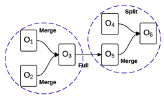
Figure 4: Example of splitting a topology into sub topologies.

The split algorithm explores the topology using multiple depth-first searches (DFS). At the beginning, only the sink operator of the given topology is in the start point set $SP$. At each iteration, we will pick an operator, $O_{s}$, from $SP$ and build a sub-topology by performing a DFS starting from $O_{s}$. If the DFS arrives at an operator $O_{i}$ whose partitioning function is incompatible with the type of the current sub-topology, it will not further traverse $O_{i}$’s downstream operators and $O_{i}$ will not be added to the current sub-topology but instead be put into $SP$. Finally the algorithm will terminate until $SP$ is empty. Figure 4 presents an example general topology, which is decomposed into two sub-topologies: $\{O_{1},O_{2},O_{3}\}$ and $\{O_{4},O_{5},O_{6}\}$.

We present details of the correlated-failure optimization algorithm for a general topology in Algorithm 5, which is referred to as the Structure Aware algorithm. The algorithm first decomposes the topology into sub-topologies which are either full topologies or structured topologies. Then the algorithm runs in multiple iterations. Within each iteration, it will try to get a replication plan from each sub-topology and select the one with the maximum profit density (lines $11-17$). The loop will be terminated when there is no more resource to replicate a complete MC-tree. The algorithm’s complexity is equal to $O(R\cdot N\cdot M^{2}\cdot E)$, where the notations are defined in Section IV-C1.

V System Implementation

V-A Framework

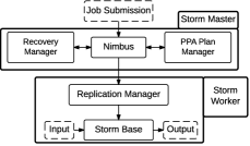
Figure 5: System Framework

We implemented our system on top of Storm. In comparing to Spark Streaming, which processes data in a micro-batching approach, Storm will process an input tuple once it arrives and thus can achieve sub-second end-to-end processing latency. As shown in Figure 5, the nimbus in the Storm master node assigns tasks to the Storm worker nodes and monitoring the failures. On receiving a job, the nimbus will transfer the query topology to the PPA plan manager, which will generate a PPA recovery plan under the constraint of resource usage of active replication. The PPA recovery plan consists of two parts: a completely passive standby plan and a partially active replication plan. Based on the PPA recovery plan, the replication manager in the worker nodes will create checkpoints to passively replicate the whole query topology. Checkpoints will be stored onto a set of standby nodes. The replication manager will create active replicas for the tasks that are included in the partially active replication plan. The active replicas can support fast failure recovery and will also be deployed onto the standby nodes.

Once a failure is detected by the nimbus, The recovery manager in the Storm master node will decide how to recover the failed tasks based on the PPA replication plan. For the tasks that are actively replicated, the recovery manager will notify the nimbus to recover them using their active replicas such that the tentative results could be produced as soon as possible. The failed tasks that are passively replicated will be recovered with their latest checkpoints.

V-B PPA Fault Tolerance

Passive Replication. In PPA, checkpoints of the processing tasks will be periodically created and stored at the standby nodes. We adopted the batch processing approach [26] to guarantee the processing ordering of inputs during recovery is identical to that before the failure. With this approach, input tuples are divided into a consecutive set of batches. A task will start processing a batch after it receives all its input tuples belonging the current batch. This is ensured by waiting a batch-over punctuation from each of its upstream neighboring tasks. Tuples within a batch will be processed in a predefined round-robin order. The effect of batch size on the system performance has been researched in previous work [6].

A single point failure can be recovered by restarting the failed task, loading its latest checkpoint and replaying its upstream tasks’ buffered data. The downstream tasks will skip the duplicated output from the recovering task until the end of the recovery phase. While recovering a correlated failure, if a task and its upstream neighboring task are failed simultaneously and its checkpoint is made later than its upstream peers’, the recovery of the downstream task can only be started after its upstream peer has caught up with the processing progress. In other words, synchronizations have to be carried out among the neighboring tasks.

Active Replication. If task $t$ has an active replica $t^{\prime}$, the output buffer of $t^{\prime}$ will store the output tuples produced by processing the same input in the same sequence as $t$ does. The downstream tasks of $t$ will subscribe the outputs from both $t$ and $t^{\prime}$. By default, the output of $t^{\prime}$ is turned off. To reduce the buffer size on $t^{\prime}$, its primary, $t$, will periodically notify $t^{\prime}$ about the latest output progress and the latter can then trim its output buffer. If $t$ is failed, $t^{\prime}$ will start sending data to the downstream tasks of $t$. The downstream tasks will eliminate the duplicated tuples from $t^{\prime}$ by recognizing their sequence numbers. The batch processing strategy can guarantee an identical processing order between the primary and active replica of a task.

Tentative Outputs. As checkpoint-based recovery requires replaying the buffered data and synchronizations among the connected tasks and hence incurs significant recovery latency, PPA has the option to continue producing tentative results once the actively replicated tasks are recovered. Recall that during normal processing, a task will only start processing a batch after receiving the batch-over punctuations from all of its upstream neighboring tasks. If any of its upstream neighboring tasks fails, the recovery manager in the Storm master node will generate the necessary batch-over punctuations for those failed tasks, such that a batch could be processed without the inputs from the failed tasks and tentative outputs will be generated with an incomplete batch. After the failed tasks are recovered, the recovery manager will stop sending the batch-over messages for them such that the downstream tasks will wait for the batch contents from the recovered tasks before processing a batch. After all the failed tasks are recovered, the topology will start generating accurate outputs.

In this paper, we assume the adoption of similar techniques proposed in [3] to reconcile the computation state and correct the tentative outputs and leave the implementation of these techniques as our future work.

V-C Dynamic Plan Adaptation

Considering that tasks’ input rates may fluctuate over time, the active replication plan should be dynamically adapted accordingly. The PPA plan manager periodically collects the input rates of all the processing tasks and generate new active replication plan. If the new plan is different from the previously applied plan, applying the new plan may require deactivating the active replicas of a set of tasks and generating active replicas for another set of tasks. Deactivating the active replicas can be implemented by terminating their processing and releasing their occupied resources. To generate new active replicas, we can send the corresponding checkpoints to the destination nodes and initialize the state of the active replicas by using the checkpoints. The newly started active replicas will receive the buffered outputs from their upstream neighboring tasks and then start the processing. Eventually, the newly generated active replicas will catch up with the progress of their primary copies. Dynamic plan adaptation is not implemented in the current version of our system, which is part of our future work.

VI Evaluation

The experiments are run over the Amazon EC2 platform. We build a cluster consisting of 36 instances, of which 35 m1.medium instances are used as the processing nodes and one c1.xlarge instance is set as the Storm master node. Heartbeats are used to detect node failures in a 5-second interval. The recovery latency is calculated as the time interval between the moment that the failure is detected and the instant when the failed task is recovered to its processing progress before failure. The processing progress of a task is defined as a vector. Each field of the progress vector contains the sequence number of the latest processed tuple from a specific input stream of the task. A failed task is marked as recovered if the values of all the fields in its current progress vector are larger than or equal to the values of the corresponding fields of the progress vector before failure. Additional information of the experiment configuration will be presented in the following sections.

VI-A Recovery Efficiency

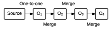
Figure 6: Topology used in the experiments of recovery efficiency in the scale of operator.

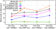
Figure 7: Recovery latency of single node failure.

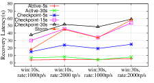
Figure 8: Recovery latency of correlated failure.

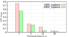
Figure 9: Resource usage of maintaining checkpoints, window length: 30 seconds.

In the first set of experiments, we study the recovery efficiencies of different fault-tolerance techniques, including checkpoint, which is used in Spark Streaming, source replay, which is the default fault-tolerance technique in Storm, and active replication. In Storm, if failure happens, the source data will be reprocessed from scratch through the whole topology to rebuild the states of the tasks.

We implement a topology that consists of 1 source operator and 4 synthetic operators. The structure of this topology is depicted in Figure 6. The source operator consists of totally 16 tasks, which are on average deployed on 4 nodes. All of the source tasks produce input tuples for their downstream neighboring tasks in a specified rate (1000 tuples/s or 2000 tuples/s). The degree of parallelization of operators $O_{1}$, $O_{2}$, $O_{3}$ and $O_{4}$ are set as 8, 4, 2 and 1 respectively. Each task in $O_{1}$ receives inputs from two source tasks and each task in $O_{2}$, $O_{3}$ and $O_{4}$ receives inputs from two upstream neighboring tasks. The primary replicas of the 15 synthetic tasks are evenly distributed among the 15 nodes. In addition, there are another 15 nodes used as the backup nodes to store the checkpoints and to run the active replicas.

Each of the four synthetic operators maintains a sliding window whose sliding step is set as 1 second and window interval varies from 10 seconds to 30 seconds. The state of each task of a synthetic operator is composed by the input data within the current window interval. The largest state size of a task is equal to the result of the input rate multiplies the window interval. The selectivity of the synthetic operator is set as $0.5$.

Single Node Failure. Figure 9 presents the recovery latencies of single node failures with various input rates and window intervals using different fault-tolerance techniques. For active replication, we vary the intervals of trimming the output buffer of a task replica, which is equivalent to the frequency of synchronizing the replica with its primary task. One can see that the active approach has much lower recovery latency than the passive approaches and the changes of window intervals and input rates have little influence. On the other hand, the recovery latencies with both Checkpoint and Storm increase proportionally with the input rate, as a higher input rate results in more tuples to be replayed during recovery for both approaches. Furthermore, the recovery latency with Checkpoint increases with the checkpoint interval. This is because the number of tuples that need be reprocessed to recover the task state will increase with the checkpoint interval.

As Storm will have to replay more source data with longer window intervals, one can see that the recovery latency of Storm with 30-second windows is higher than those with 10-second windows. Another factor that influences the recovery latency of Storm is the location of the failed task in the topology, because the replayed tuples will be processed by all the tasks located between the tasks of the source operator and the failed tasks. Thus the recovery latency of Storm is higher than that of Checkpoint in most of the cases in this experiment. Here, we record the recovery latencies of tasks in different locations within the topology in Storm and report their average values.

Correlated Failure. We inject a correlated failure by killing all the nodes on which the primary replicas of the tasks are deployed. In Figure 9, one can see that active replication has much lower recovery latency than Checkpoint and Storm. Furthermore, active replication with a shorter synchronization period leads to faster failure recovery. This is because, with a longer synchronization period, an active replica will send more buffered tuples to its downstream tasks if its primary is failed. On the other hand, the recovery latency of Checkpoint increases rapidly with the increase of input rate and checkpoint interval. Storm has a lower recovery latency than that of Checkpoint with a 30-second checkpoint interval. This is because the window intervals in this set of experiments are relatively short. In Storm, to build the window states, all the sources tuples belonging to the unfinished window instances in the failed tasks will be replayed, whose number increases linearly with the window length. While for the recovery with Checkpoint, the number of tuples that should be reprocessed to recover a failed task is at most equal to the value of the input rate multiplies the checkpoint interval.

By comparing the experimental results presented in Figure 9 and Figure 9, it can be seen that the recovery latency with active replication is lower than the passive approaches and is relatively stable under the scenarios of various input rates and window intervals. Moreover, the benefits of using active replication are larger in the case of correlated failure than in the case of single node failure. This is because some synchronization operations will be performed during the recovery of correlated failures.

The latency of failure recovery with checkpoint can be reduced by setting a short checkpoint interval. However, the resource usage of maintaining checkpoints varies with different checkpoint intervals. Figure 9 presents the ratio of the CPU usage of maintaining checkpoint to that of normal computation within a task. We can see that the CPU usage of maintaining checkpoints increases quickly with shorter checkpoint intervals and making checkpoint with very short intervals such as one second is prohibitively expensive. Although active replication consumes more recourses than the passive approach, the low-latency recovery of active replication makes it meaningful in the context of MPSPEs.

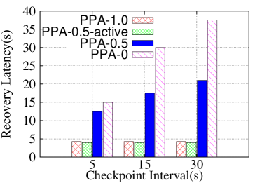
(a) rate:1000 tuples / sec

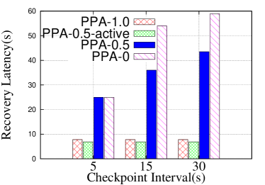
(b) rate:2000 tuples / sec

Figure 10: Recovery latency of a correlated failure with PPA, window length : 30 seconds. PPA-0.5-active indicates the recovery latency of actively replicated tasks in plan PPA-0.5.

Recovery with PPA. We conducted experiments to study the performance of PPA with three active replication plans denoted as PPA-1.0, PPA-0.5 and PPA-0 respectively. These PPA plans consume various amount of resources for active replication. In PPA-1.0, all the tasks in the topology will be actively replicated. PPA-0.5 is a hybrid replication plan where only half of the tasks have active replica. PPA-0 is a purely passive replication plan where all the tasks are only replicated with checkpoint. The results are presented in Figure 10. As the failed tasks with active replicas will be recovered faster than those using checkpoints, the overall recovery latency of PPA-0.5 is higher than that of PPA-1.0 but lower than that of PPA-0. Note that with PPA-0.5, the recovery latencies of tasks with active replicas (denoted as PPA-0.5-active in Figure 10) are much lower than that of recovering all the failed tasks (denoted as PPA-0.5 in Figure 10). The recoveries of PPA-0.5-active consume slightly less time than PPA-1.0, this is because the number of actively replicated tasks recovered in PPA-0.5-active is only the half of that in PPA-1.0. This set of experiments illustrate that the purely active replication plan outperforms the hybrid and purely passive plan regarding the recovery latency. With a hybrid plan, as the recoveries of actively replicated tasks finish earlier than that of the passively replicated ones, PPA can generate tentative outputs without waiting for the slow recoveries of passively replicated tasks.

VI-B Tentative Output Quality

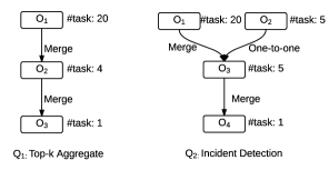
Figure 11: Top-k aggregate query$(Q_{1})$ and incident detection query$(Q_{2})$ in the scale of operator.

We implement two sliding window queries whose inputs are, respectively, from real and synthetic datasets. For each query, we define an accuracy function based on its semantic.

$Q_{1}$ is a sliding-window query that calculates the top-100 hottest entries of the official website of World Cup 1998. The input dataset is the server access log during the entire day of June 30, 1998 [1], which consists of in total $73,291,868$ access records. In the experiments, we replay the raw input stream in a rate which is $48$ times faster than the original data rate. We implement this query as a topology that conducts hierarchical aggregates, which is a common computation in data stream applications. The structure of this topology is depicted in Figure 11. Input tuples are partitioned to the tasks in $O_{1}$ by their server ids. Tasks in $O_{1}$ split the input stream into a set of consecutive slices, each consisting of 100 tuples, and calculate their aggregate results. For every 100 input tuples, tasks in $O_{2}$ will conduct a merge computation and send the results to the single task in $O_{3}$, which periodically updates the globally top-100 entries for every 100 input tuples.

$Q_{2}$ is a sliding-window query that detects the traffic incidents resulting in traffic jams. The window interval is 5 minutes and the sliding step is 10 seconds. As relevant datasets for this query are not publicly available due to privacy considerations, we generate a synthetic dataset in a community-based navigation application. There are two streams in this dataset: the user-location stream and the incident stream. The rate of the user-location stream is set as 20,000 location records per second. The incident stream is composed of user-reported incident events and the time interval between two consecutive incidents is set as 2 seconds. We distribute 100,000 users among 1000 virtual road segments following the Zipfian distribution (with parameter $s=0.5$). The incident probability of a segment is set to be proportional to the number of users located on it. If an incident occurs on a segment, all the users on this segment will report an incident event. The topology of $Q_{2}$ is presented in Figure 11. Tasks in $O_{1}$ receive the user-location records and calculate the average speed of each segment per second. Tasks in $O_{2}$ combine the user-reported incident events into distinct incident events. $O_{3}$ joins the segment-speed stream from $O_{1}$ and the distinct-incident stream from $O_{2}$. The outputs of tasks in $O_{3}$ are the incidents that incur traffic jams. $O_{4}$ aggregates the outputs of $O_{3}$.

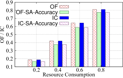
(a) Query: Q1.

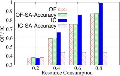
(b) Query: Q2.

Figure 12: Comparing the values of OF/IC and the query accuracy. OF-SA-Accuracy (or IC-SA-Accuracy) denotes the actual query accuracies of the PPA plans generated using the structure-aware(SA) algorithm with OF (or IC) as the optimization metric.

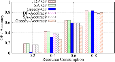
(a) Query: Q1.

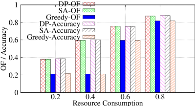
(b) Query: Q2.

Figure 13: Comparing the values of OF and the actual query accuracies of the PPA plans which are generated by the dynamic programing algorithm(DP), structure-aware algorithm(SA) and greedy algorithm(Greedy) respectively.

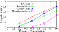
(a) Workload skewness

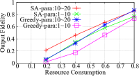
(b) Degree of parallelization

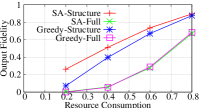
(c) Full partitioning

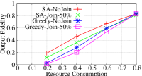
(d) Fraction of join operators

Figure 14: Comparing OF of SA and Greedy algorithm with random topologies of various specifications, number of operators is set as a random integer between $5$ and $10$. (a): The workloads of tasks within an operator are distributed in uniform or Zipfian distribution (with parameter $s=0.1$). (b): The degree of operator parallelization is a random number between different ranges. (c): Topologies are either structured topology or full topology. (d): The fraction of join operators in the topologies is set as $0$ or $50\%$.

Validation of the OF metric. In this set of experiments, we examine whether OF can predict the actual quality of the tentative output. We compare it with the Internal Completeness $\left(IC\right)$ metric proposed in [4], which measures the fraction of the tuples that are expected to be processed by all the tasks in case of failures compared to the case without failures. A fundamental difference between OF and IC is that, OF takes the correlations of task’s input streams into account.

By denoting the tentative outputs as $S_{T}$ and the accurate outputs of $Q_{1}$ as $S_{A}$, we define the query accuracy of $Q_{1}$ as: $\frac{|S_{T}\bigcap S_{A}|}{|S_{A}|}$. Figure 12(a) shows the OF (or IC) values and the actual query accuracies of the PPA plans generated using the OF (or IC) metric. The results show that both OF and IC provide good predictions of the accuracy of typical top-k queries. This is because both OF and IC provide accurate estimations of the completeness of the inputs for aggregate queries, such as top-k, and such queries’ output accuracies highly depend on the completeness of their inputs. The accuracy function of $Q_{2}$ is defined as $\frac{|I_{T}\bigcap I_{A}|}{|I_{A}|}$, where $I_{T}$ is the set of tentative incidents generated with correlated failure and $I_{A}$ is the set of accurate incidents generated without failure. As shown in Figure 12(b), the accuracy values are generally quite close to the values of OF. On the other hand, with more available resources, we can generate PPA plans with higher IC values. However, such plans do not have higher query accuracies. This is because IC fails to consider the correlation of tasks’ input streams and hence cannot provide a good accuracy prediction for queries with joins. This result clearly indicates the importance of distinguishing join operators in predicting output accuracies.

Comparing Various Algorithms. In this set of experiments, we generate PPA plans for $Q_{1}$ and $Q_{2}$ using the dynamic programing algorithm(DP), the structure-aware algorithm(SA) and the greedy algorithm respectively and compare their performances. Results presented in Figure 13 show that SA is quite close to DP, which generates the optimal PPA plan, in both OF and the actual query accuracy. Greedy has the worst performance in the results of both queries. This is because Greedy fails to consider that only complete MC-trees can contribute to the query outputs.

VI-C Random synthetic topology

To conduct a comprehensive performance study of PPA algorithms with various types of topologies, we implemented a random topology generator which can generate topologies with different specifications. In the experiments, for each set of topology specifications, we generate 100 synthetic topologies and use them as the inputs of the structure-aware algorithm and the greedy algorithm to compare their performances in terms of OF. Due to the prohibitive complexity of the dynamic programing algorithm, we cannot complete it for this set of experiments within a reasonable time so we do not include it here. Query accuracies are not compared in this set of experiments, as we cannot derive the actual output accuracies for these randomized synthetic topologies.

In Figure 14, one can see that, SA outperforms the greedy algorithm in all the combinations of topology specifications and active replication ratios. With smaller replication ratio, there is a greater difference between SA and the greedy algorithm. This is because the greedy algorithm is agnostic to the structure of the query topologies, and with a smaller replication ratio, there is smaller probability that the tasks selected by the greedy algorithms can form complete MC-trees that can contribute to the final output.

Figure 14(a) depicts the effects of workload skewness of tasks within the operators. We can see that SA has better performance for topologies that have higher skewness of task workloads. This is because, as the skewness of workloads increases, the skewness of MC-trees’ contributions to the value of OF also increases and SA, by prioritizing tasks that are in the MC-trees, achieves higher OF values. In Figure 14(b), we report the results with varying parallelization degrees of an operator. One can see that increasing the parallelization degrees will also increase the value of OF, because a higher parallelization degree slightly increases the skewness of the workloads of the tasks in this set of experiments. As shown in Figure 14(c), the OF of structured topologies are generally higher than the full topologies. This is because within an operator using Full partitioning, the failure of any task will reduce the input of all the downstream tasks. For full topologies, the structure-aware algorithm generates active replication plan in the similar approach as the greedy algorithm does, thus their performances are close in this set of experiments. Figure 14(d) presents the results with various fractions of operators being join operators. For the same topology, OF decreases with more operators set as joins. This is because the loss of one input stream of a join operator will result in parts of the other (correlated) input streams being useless.

VII Related Work

Fault-tolerance in SPE. Traditional fault-tolerance techniques for SPEs could be categorized as passive  [13, 25, 17, 19, 18] and active approaches [13, 3, 12]. The technique of delta checkpoint [14] is used to reduce the size of checkpoints. The authors in [9] proposed techniques to reduce the checkpoint overhead by minimizing the sizes of queues between operators, which are part of the checkpoints. [20] proposed to utilize the idle period of the processing nodes for active replication. Such optimizations are compatible to our PPA scheme and can be employed in our system.

Spark Streaming [26] uses Resilient Distributed Dataset (RDD) to store the states of processing tasks. In case of failure, RDDs can be restored from checkpoints or rebuilt by performing operations that were used to build it based on its lineage. In other words, it adopts both the checkpoint-based and the replay-based approaches.

For other large-scale computing systems, such as Map-Reduce [7], the overall job execution time is a critical metric. However, for MPSPEs, it is the end-to-end latency of tuple processing that matters, which makes the low-latency failure recovery an important feature in the context of MPSPEs. To reduce recovery latency, authors in [5, 26] proposed to use parallel recovery and/or integrating fault tolerance with scale-out operations. In parallel recovery, multiple tasks can be launched to recover a failed task and each of them is recovering a partition of the failed one to shorten the process of passive recovery. However, with a correlated failure, a large number of failed tasks need to be recovered simultaneously. Then the possibilities of fast scaling out and the degrees of parallel recovery would be constrained.

Hybrid fault-tolerance approaches are proposed in [25, 11]. In [25], the objective is to minimize the total cost by choosing a passive fault-tolerance strategy, including upstream buffering, local checkpoint and remote checkpoint, for each operator. [11] uses either active replication or checkpoint as the fault-tolerance approach for an operator. The optimization objective in [11] is to minimize the total processing cost while satisfying the user-specified threshold of recovery latency, where only independent failure is considered. The work in [27] considers task overloading, referred to as “transient” failure, caused by temporary workload spikes. Upon a transient failure of a task, its active replica will be used to generate low-latency output. Different from these approaches, the trade-off of our work is between resource consumption and result accuracy with correlated failures.

Tentative Outputs. Borealis [3] uses active replication for fault tolerance and allows users to trade result latency for accuracy while the system is recovering from a failure. More specifically, if a failed node has no alive replica, Borealis will produce tentative outputs if the recovery cannot be finished within a user-defined interval. PPA adopts a similar mechanism for generating tentative outputs but explores more on optimizing the accuracy of tentative results. Previous work [4] attempts to dynamically assign computation resources between primary computation and active replicas to achieve trade-offs between system throughput and fault-tolerance guarantee. Their accuracy model, IC, does not consider the correlation of processing tasks’ inputs streams, which is shown to be inadequate in our experiments. The brute-force algorithm proposed in [4] which has a high complexity as our dynamic programing does.

A fault injection-based approach is presented in [15] to evaluate the importance of the computation units to the output accuracy, which only considers independent failures. Zen [22] optimizes operator placement within clusters under a correlated failure model, which specifies the probability that a subset of the nodes fail together. The objective is to maximize the accuracy of tentative outputs after failures. As operator placement is orthogonal to the planning of active replications, their techniques can also be employed as a supplement to PPA.

Failure in Clusters. Previous studies found that failure rates vary among different clusters and the number of failures is in general proportional to the size of the cluster [23]. Correlated failures do exist and their scopes could be quite large [10, 21]. Hence considering correlated failure is inevitable for a MPSPE that supports low-latency and nonstop computations.

VIII Conclusion

In this paper we present a passive and partially active (PPA) fault-tolerance scheme for MPSPEs. In PPA, passive checkpoints are used to provide fault-tolerance for all the tasks, while active replications are only applied to selective ones according to the availability of resources. A partially active replication plan is optimized to maximize the accuracy of tentative outputs during failure recovery. The experimental results indicate that upon a correlated failure, PPA can start producing tentative outputs up to 10 times faster than the completion of recovering all the failed tasks. Hence PPA is suitable for applications that prefer tentative outputs with minimum delay. The experiments also show that our structure-aware algorithms can achieve up to one order of magnitude improvements on the qualities of tentative outputs in comparing the greedy algorithm that is agnostic to query topology structures, especially when there is limited resource available for active replications. Therefore, to optimize PPA, it is critical to take advantage of the knowledge of the query topology’s structure.

References

- [1] http://ita.ee.lbl.gov.
- [2] B. Babcock, M. Datar, et al. Load shedding for aggregation queries over data streams. ICDE’04.
- [3] M. Balazinska, H. Balakrishnan, et al. Fault-tolerance in the borealis distributed stream processing system. ACM Trans. Database Syst, 2008.
- [4] P. Bellavista, A. Corradi, et al. Adaptive fault-tolerance for dynamic resource provisioning in distributed stream processing systems. In EDBT’14.
- [5] F. Castro, M. Raul, et al. Integrating scale out and fault tolerance in stream processing using operator state management. SIGMOD’13.
- [6] T. Das, Y. Zhong, et al. Adaptive stream processing using dynamic batch sizing. Master Thesis’2014.
- [7] J. Dean and S. Ghemawat. Mapreduce: simplified data processing on large clusters. Communications of the ACM, 51(1):107–113, 2008.
- [8] O. Goldschmidt, D. Nehme, and G. Yu. Note: On the set-union knapsack problem. Naval Research Logistics (NRL), 41(6):833–842, 1994.
- [9] Y. Gu, Z. Zhang, et al. An empirical study of high availability in stream processing systems. Middleware’09.
- [10] T. Heath, R. P. Martin, et al. Improving cluster availability using workstation validation. SIGMETRICS’02.
- [11] T. Heinze, M. Zia, et al. An adaptive replication scheme for elastic data stream processing systems. DEBS ’15.
- [12] J.-H. Hwang, U. Cetintemel, and others. Fast and highly-available stream processing over wide area networks.
- [13] J.-H. Hwang et al. High-availability algorithms for distributed stream processing. ICDE’05.
- [14] J.-H. Hwang, Y. Xing, et al. A cooperative, self-configuring high-availability solution for stream processing. ICDE’07.
- [15] G. Jacques-Silva, B. Gedik, et al. Fault injection-based assessment of partial fault tolerance in stream processing applications. DEBS’11.
- [16] J. Kang, J. F. Naughton, et al. Evaluating window joins over unbounded streams. ICDE’03.
- [17] Y. Kwon, M. Balazinska, et al. Fault-tolerant stream processing using a distributed, replicated file system.
- [18] K. G. S. Madsen, P. Thyssen, and Y. Zhou. Integrating fault-tolerance and elasticity in a distributed data stream processing system. SSDBM ’14.
- [19] K. G. S. Madsen and Y. Zhou. Dynamic resource management in a massively parallel stream processing engine. CIKM ’15.
- [20] A. Martin, C. Fetzer, and A. Brito. Active replication at (almost) no cost. SRDS’11.
- [21] S. Nath, H. Yu, Gibbons, et al. Subtleties in tolerating correlated failures in wide-area storage systems. NSDI’06.
- [22] B. Nikhil, B. Ranjita, et al. Towards optimal resource allocation in partial-fault tolerant applications. In INFOCOM’08.
- [23] B. Schroeder and G. A. Gibson. A large-scale study of failures in high-performance computing systems. DSN’06.
- [24] A. Toshniwal, S. Taneja, et al. Storm@twitter. SIGMOD ’14.
- [25] P. Upadhyaya, Y. Kwon, et al. A latency and fault-tolerance optimizer for online parallel query plans. SIGMOD’11.
- [26] M. Zaharia et al. Discretized streams: Fault-tolerant streaming computation at scale. SOSP ’13.
- [27] Z. Zhang, Y. Gu, et al. A hybrid approach to high availability in stream processing systems. ICDCS ’10.
- [28] J. Zhou et al. Advanced partitioning techniques for massively distributed computation. SIGMOD’12.