$N$-coherence vs. $t$-coherence:
An alternative route to the Gross-Pitaevskii equation

Abstract

We show how a candidate mean-field amplitude can be constructed from the exact wave function of an externally forced $N$-Boson system. The construction makes use of subsidiary $(N-1)$-particle states which are propagated in time in addition to the true $N$-particle state, but does not involve spontaneous breaking of the $U(1)$ symmetry associated with particle number conservation. Provided the flow in Fock space possesses a property which we call maximum stiffness, or $t$-coherence, the candidate amplitude actually satisfies the time-dependent Gross-Pitaevskii equation, and then serves as macroscopic wave function of the forced $N$-particle system. The general procedure is illustrated in detail by numerical calculations performed for the model of a driven bosonic Josephson junction, which allows one to keep track of all contributions which usually are subject to uncontrolled assumptions. These calculations indicate that macroscopic wave functions can persist even under conditions of strong forcing, but are rapidly destroyed upon entering a regime of chaotic dynamics. Our results provide a foundation for future attempts to manipulate, and actively control, macroscopic wave functions by means of purposefully designed force protocols.

I Introduction and Overview

This paper concerns the time evolution of a system of $N$ interacting identical spinless Bose particles of mass $m$, where $N$ is assumed to be large. At each moment $t$ in time it is described by a Schrödinger wave function $\Psi$ which is symmetric in all its spatial arguments,

$$\Psi(\bm{r}_{1},\ldots,\bm{r}_{N};t)=\Psi(\bm{r}_{P(1)},\ldots,\bm{r}_{P(N)};t)$$ (1)

for each permutation $P$ of the indices $1,\ldots,N$. Its dynamics are governed by an $N$-particle Schrödinger equation

$${\mathrm{i}}\hbar\frac{\partial}{\partial t}\Psi(\bm{r}_{1},\ldots,\bm{r}_{N};t)$$

$$= \left[\sum_{j=1}^{N}h_{1}(\bm{r}_{j};t)+\frac{1}{2}\sum_{j\neq k}U(\bm{r}_{j},\bm{r}_{k})\right]\Psi(\bm{r}_{1},\ldots,\bm{r}_{N};t)\;,$$

where

$$h_{1}(\bm{r};t)=-\frac{\hbar^{2}}{2m}\Delta+V(\bm{r};t)$$ (3)

denotes a single-particle Hamiltonian containing an external potential $V$ which may depend explicitly on time, so as to exert some controlling influence on the system, and the interparticle interaction $U$ naturally is symmetric,

$$U(\bm{r},\bm{r}^{\prime})=U(\bm{r}^{\prime},\bm{r})\;.$$ (4)

We will assume that $U$ can be replaced by an effective contact interaction with strength $g$,

$$U_{\rm eff}(\bm{r},\bm{r}^{\prime})=g\,\delta(\bm{r}-\bm{r}^{\prime})\;,$$ (5)

which means that we restrict ourselves to the low-energy regime HuangYang57 .

The central question addressed in this work is under what conditions an approximate description of the dynamics in terms of a mean-field amplitude $\Phi$ evolving according to the time-dependent Gross-Pitaevskii equation Gross61 ; Pitaevskii61 ; Gross63 ; Gardiner97 ; CastinDum98 ; Leggett01 ; PethickSmith08 ; PitaevskiiStringari03 is viable, and, if so, how that amplitude is related to the actual wave function $\Psi$. Since $\Phi=\Phi(\bm{r};t)$ depends on only one spatial coordinate $\bm{r}$, it contains much less information than the many-body wave function (1) could possibly carry. Therefore, a reduction of the full $N$-particle dynamics to the mean-field level without essential loss of information is feasible only if already the $N$-particle wave function itself is relatively simple, or ordered, so that the mean-field amplitude, if it exists, may be regarded as an order parameter of the system Leggett00 . According to common knowledge deriving from London’s theory of superfluids London64 the mean-field amplitude should correspond to a “macroscopic wave function”, that is, to a macroscopically occupied single-particle orbital. This is fully in line with the preservation of information: In the ideal case where all $N$ particles occupy the same orbital, no information is lost if $\Phi(\bm{r};t)$ equals that orbital. But this leads to further questions when the system is subjected to time-dependent forcing: Even if the initial state is given exactly by an $N$-fold occupied single-particle orbital, this initial order might be destroyed by the external force, and the time-dependent many-particle state may become arbitrarily complicated, no longer admitting a mean-field description. On the other hand, one may formally solve the Gross-Pitaevskii equation with an arbitrary type of external forcing incorporated into the single-particle Hamiltonian $h_{1}$. Hence, there must be some sort of indicator which tells one whether or not the solution to the time-dependent Gross-Pitaevskii equation can actually serve as a macroscopic wave function of the forced $N$-particle system. Here we explore this intuitive idea in mathematical terms.

As a guideline for the following deliberations, and to state the subject as clearly as possible, we briefly sketch a popular pseudo-derivation of the Gross-Pitaevskii equation. To this end, we introduce the usual Fock space annihilation and creation operators $\widehat{\psi}(\bm{r})$ and $\widehat{\psi}^{\dagger}(\bm{r})$ which obey the canonical Bose commutation relations

$$\left[\widehat{\psi}(\bm{r}),\widehat{\psi}(\bm{r}^{\prime})\right] = 0$$

$$\left[\widehat{\psi}^{\dagger}(\bm{r}),\widehat{\psi}^{\dagger}(\bm{r}^{\prime})\right] = 0$$

$$\left[\widehat{\psi}(\bm{r}),\widehat{\psi}^{\dagger}(\bm{r}^{\prime})\right] = \delta(\bm{r}-\bm{r}^{\prime})\;,$$ (6)

so that the Fock-space many-body Hamiltonian takes the form Fock32

$$\widehat{H}(t) = \int\!{\mathrm{d}}^{3}r\,\widehat{\psi}^{\dagger}(\bm{r})h_{1}(\bm{r};t)\widehat{\psi}(\bm{r})$$

$$+ \frac{1}{2}\int\!{\mathrm{d}}^{3}r\!\int\!{\mathrm{d}}^{3}r^{\prime}\,\widehat{\psi}^{\dagger}(\bm{r})\widehat{\psi}^{\dagger}(\bm{r}^{\prime})U(\bm{r},\bm{r}^{\prime})\widehat{\psi}(\bm{r}^{\prime})\widehat{\psi}(\bm{r})\;.$$

Here we use the “hat”-symbol to designate operators acting in Fock space, in contrast to single-particle operators such as the one given by Eq. (3).

With the help of the unitary operator $\widehat{U}(t,t_{0})$ which effectuates the time evolution from some initial moment $t_{0}$ to $t$ and thus obeys the equation

$${\mathrm{i}}\hbar\frac{{\mathrm{d}}}{{\mathrm{d}}t}\widehat{U}(t,t_{0})=\widehat{H}(t)\widehat{U}(t,t_{0})\;,$$ (8)

the field operator $\widehat{\psi}(\bm{r})$ is transformed to the Heisenberg picture through the familiar prescription

$$\widehat{\psi}_{\rm H}^{\phantom{\dagger}}(\bm{r};t)=\widehat{U}^{\dagger}(t,t_{0})\widehat{\psi}(\bm{r})\widehat{U}(t,t_{0})\;,$$ (9)

leading to an equation of motion of the form

$${\mathrm{i}}\hbar\frac{{\mathrm{d}}}{{\mathrm{d}}t}\widehat{\psi}_{\rm H}^{\phantom{\dagger}}(\bm{r};t)=\widehat{U}^{\dagger}(t,t_{0})\left[\widehat{\psi}(\bm{r};t),\widehat{H}(t)\right]\widehat{U}(t,t_{0})\;.$$ (10)

Working out the commutator appearing on the right-hand side, one obtains

$${\mathrm{i}}\hbar\frac{{\mathrm{d}}}{{\mathrm{d}}t}\widehat{\psi}_{\rm H}^{\phantom{\dagger}}(\bm{r};t) = h_{1}(\bm{r};t)\widehat{\psi}_{\rm H}^{\phantom{\dagger}}(\bm{r};t)$$

$$+ \!\!\!\!\int\!{\mathrm{d}}^{3}r^{\prime}\,\widehat{\psi}_{\rm H}^{\dagger}(\bm{r}^{\prime};t)U(\bm{r},\bm{r}^{\prime})\widehat{\psi}_{\rm H}^{\phantom{\dagger}}(\bm{r}^{\prime};t)\widehat{\psi}_{\rm H}^{\phantom{\dagger}}(\bm{r};t)\;;$$

inserting the contact potential (5), one is left with

$${\mathrm{i}}\hbar\frac{{\mathrm{d}}}{{\mathrm{d}}t}\widehat{\psi}_{\rm H}(\bm{r};t) = h_{1}(\bm{r};t)\widehat{\psi}_{\rm H}(\bm{r};t)$$

$$+ g\,\widehat{\psi}^{\dagger}_{\rm H}(\bm{r};t)\widehat{\psi}_{\rm H}(\bm{r};t)\widehat{\psi}_{\rm H}(\bm{r};t)\;.$$

Now comes a major assumption: The mean-field amplitude $\Phi$ is supposed to be given by the expectation value of the Heisenberg field operator,

$$\sqrt{N}\Phi(\bm{r};t):=\left\langle\widehat{\psi}_{\rm H}(\bm{r};t)\right\rangle\;.$$ (13)

This definition requires clarification. If it is taken literally, each $N$-particle state $|\Psi\rangle_{N}$, no matter how “simple”, can only produce a left-hand side equal to zero, since the $(N-1)$-particle state $\widehat{\psi}_{\rm H}(\bm{r};t)|\Psi\rangle_{N}$ is orthogonal to $|\Psi\rangle_{N}$ in Fock space. Hence, when working with Eq. (13) one supposes that the superselection rule for the total particle number $N$ is somehow violated, and the state $|\Psi\rangle$ with respect to which the expectation values (13) are taken is some coherent superposition of $N$-particle states $|\Psi\rangle_{N}$ with different $N$,

$$|\Psi\rangle=\sum_{N}a_{N}|\Psi\rangle_{N}\;.$$ (14)

This corresponds to the idea that the $U(1)$ symmetry associated with particle number conservation is spontaneously broken. While that concept may be helpful for simplifying formal calculations, it remains an auxiliary device not rooted on the grounds of the actually given $N$-particle system. This deficiency has led to several profound discussions in the literature, and to the development of number-conserving approaches Gardiner97 ; CastinDum98 ; Leggett01 ; GirardeauArnowitt59 ; Girardeau98 ; GardinerMorgan07 . The unreflected use of the notion of spontaneous symmetry breaking has been severely challenged by Leggett, who criticizes that there are no circumstances in which Eq. (14) is the physically correct description of the system, and maintains that the definition (13) is “liable to generate pseudoproblems, and is best avoided” Leggett01 . Thus, one of the goals of the present study is to provide an alternative, logically more transparent definition of the mean-field amplitude for an $N$-Boson system. In contrast to customary analysis, our approach does not involve a splitting of the field operator into a condensate part and a remainder. Instead, we will first introduce a candidate mean-field amplitude by taking matrix elements of the field operator with the physical $N$-particle state and certain auxiliary $(N-1)$-particle states, and then provide a criterion which decides whether or not that candidate is physically meaningful, so that it qualifies as a macroscopic wave function.

Still staying within the framework of spontaneously broken symmetry, an appealing possibility to satisfy Eq. (13) seems to arise when $|\Psi\rangle$ is a coherent state, which, by definition, is an eigenstate of the annihilation operator:

$$\widehat{\psi}_{\rm H}({\bm{r}};t_{0})|\Psi\rangle=\sqrt{N}\Phi({\bm{r}};t_{0})|\Psi\rangle\;,$$ (15)

or, upon return to the Schrödinger picture,

$$\widehat{\psi}(\bm{r})|\Psi(t_{0})\rangle=\sqrt{N}\Phi({\bm{r}};t_{0})|\Psi(t_{0})\rangle\;;$$ (16)

in this respect such many-body coherent states are analogs of the familiar standard harmonic-oscillator coherent states already introduced in the early days of quantum mechanics Schrodinger26 ; Schiff68 . Intuitively speaking, Eq. (15) means that $|\Psi\rangle$ is “simple” in the sense that it remains unchanged if one particle is removed. However, if $|\Psi\rangle$ is an eigenstate of $\widehat{\psi}_{\rm H}({\bm{r}};t_{0})$ at one particular moment $t_{0}$, it will not, in general, be one at others. Therefore, we are confronted with the necessity to admit more general concepts of “coherence”.

Following the traditional route for the time being and taking the symmetry-broken expectation value (13), Eq. (I) immediately yields

$${\mathrm{i}}\hbar\frac{{\mathrm{d}}}{{\mathrm{d}}t}\sqrt{N}\Phi(\bm{r};t) = h_{1}(\bm{r};t)\sqrt{N}\Phi(\bm{r};t)$$

$$+ g\left\langle\widehat{\psi}^{\dagger}_{\rm H}(\bm{r};t)\widehat{\psi}_{\rm H}(\bm{r};t)\widehat{\psi}_{\rm H}(\bm{r};t)\right\rangle\;.$$

This leads to another pertinent problem: Of course one could write down the equation of motion for the third moment appearing here, but this would involve still higher moments, and so on, leading to an infinite chain of equations expressing an infinite momentum hierarchy KohlerBurnett02 ; ErdosEtAl06 . The Gross-Pitaevskii equation results from the assumption that this chain can be terminated at the lowest possible level, so that the expectation value of the triple operator product is replaced by the product of the expectation values of the individual operators:

$$\left\langle\widehat{\psi}^{\dagger}_{\rm H}(\bm{r};t)\widehat{\psi}_{\rm H}(\bm{r};t)\widehat{\psi}_{\rm H}(\bm{r};t)\right\rangle$$ (18)

$$\leadsto \left\langle\widehat{\psi}^{\dagger}_{\rm H}(\bm{r};t)\right\rangle\left\langle\widehat{\psi}_{\rm H}(\bm{r};t)\right\rangle\left\langle\widehat{\psi}_{\rm H}(\bm{r};t)\right\rangle\;.$$

Here the “$\leadsto$”-sign is meant to indicate that this closure hypothesis (18) generally constitutes an uncontrolled approximation; note, however, that it would be exact for a coherent state (15). Accepting this factorization, Eq. (I) finally turns into the celebrated Gross-Pitaevskii equation Gross61 ; Pitaevskii61 ; Gross63 ; Gardiner97 ; CastinDum98 ; Leggett01 ; PethickSmith08 ; PitaevskiiStringari03 ; ErdosEtAl06 ; ErdosEtAl07 ; ErdosEtAl09 ; ErdosEtAl10 , namely,

$${\mathrm{i}}\hbar\frac{{\mathrm{d}}}{{\mathrm{d}}t}\Phi(\bm{r};t)=h_{1}(\bm{r};t)\Phi(\bm{r};t)+Ng|\Phi(\bm{r};t)|^{2}\Phi(\bm{r};t)\;.$$ (19)

Since one has the identity

$$\int\!{\mathrm{d}}^{3}r\left\langle\widehat{\psi}^{\dagger}_{\rm H}(\bm{r};t)\widehat{\psi}_{\rm H}(\bm{r};t)\right\rangle=N$$ (20)

for any $t$, one deduces from the definition (13) that the mean-field amplitude is normalized to unity,

$$\int\!{\mathrm{d}}^{3}r\,|\Phi(\bm{r};t)|^{2}=1\;,$$ (21)

now assuming factorization of the expectation value (20).

Besides providing an alternative definition of the mean-field amplitude not based on spontaneous breach of symmetry, questioning and monitoring the accuracy of the required closure hypothesis constitutes a main objective of this work.

We proceed as follows: In Sec. II we outline a tentative construction process of a candidate mean-field amplitude associated with an $N$-particle state $|\Psi(t)\rangle_{N}$. This construction rests on the introduction of subsidiary $(N-1)$-particle states $|\widetilde{\Psi}(\bm{r}|t)\rangle_{N-1}$ which are obtained from $|\Psi(t)\rangle_{N}$ by the annihilation of one particle; the dynamics of these states are governed by the same Hamiltonian as those of the physical state $|\Psi(t)\rangle_{N}$. Our approach is similar in spirit to the introduction of a condensate wave function by Lifshitz and Pitaevskii in Ref. LaLifIX , but places particular emphasis on the way the initially “neighboring” states $|\Psi(t)\rangle_{N}$ and $|\widetilde{\Psi}(\bm{r}|t)\rangle_{N-1}$ evolve in time: Do they, in a suitable sense, remain close to each other? The subsequent derivation of the candidate’s equation of motion then makes clear under what conditions the Gross-Pitaevskii equation (19) is satisfied, so that the construction yields a bona fide macroscopic wave function. If, on the other hand, these conditions are not met, the candidate bears no physical meaning and has to be discarded. These considerations are not meant as a substitute for rigorous mathematical analysis ErdosEtAl06 ; ErdosEtAl07 ; ErdosEtAl09 ; ErdosEtAl10 , but rather as an elaboration of the salient features which make the Gross-Pitaevskii equation work. In particular, we isolate a notion of coherence which does not correspond, in the first place, to a single-particle orbital being macroscopically occupied, but which places a certain demand on the flow in Fock space instead, requiring its stiffness.

The general scheme is applied in Sec. III to a numerically tractable model system, describing a driven Josephson junction. The model is presented in Sec. III.1, and the corresponding equations of motion are derived in Sec. III.2, now paying particular attention to keeping all error terms. The results of selected numerical calculations which support our reasoning in considerable detail are discussed at length in Sec. III.3. Besides being paradigmatically simple, the model has the further pleasant feature that it lends itself to a semiclassical interpretation, allowing one to relate the $N$-particle dynamics to those of a driven nonlinear pendulum. As laid out in Sec. III.4, this semiclassical view leads to important qualitative insights which may guide the analysis of more complicated, experimentally accessible systems in the future. Thus, the model calculations collected in this Sec. III complement recent studies of periodically $\delta$-kicked Bose-Einstein condensates which aim at exploring nonlinear dynamics in a quantum many-body context ZhangEtAl04 ; LiuEtAl06 ; DuffyEtAl04 ; WimbergerEtAl05 ; BillamGardiner12 ; BillamEtAl13 ; here we emphasize the potential usefulness of a sinusoidal force with a slowly varying envelope.

We finally phrase our main findings, and draw some general conclusions, in Sec. IV.

II Constructive approach to the mean-field amplitude

We start by constructing the $N$-particle Fock-space state vector $|\Psi(t)\rangle_{N}$ corresponding to some given wave function $\Psi$: Building on a vacuum state $|{\rm vac}\rangle$ characterized by

$$\langle{\rm vac}|{\rm vac}\rangle=1$$ (22)

and

$$\widehat{\psi}(\bm{r})|{\rm vac}\rangle=0\quad\text{for each }\bm{r}\;,$$ (23)

we have

$$|\Psi(t)\rangle_{N} = \frac{1}{\sqrt{N!}}\int\!{\mathrm{d}}^{3}r_{1}\ldots\int\!{\mathrm{d}}^{3}r_{N}\,\Psi(\bm{r}_{1},\ldots,\bm{r}_{N};t)$$ (24)

$$\times\;\widehat{\psi}^{\dagger}(\bm{r}_{1})\ldots\widehat{\psi}^{\dagger}(\bm{r}_{N})|{\rm vac}\rangle\;.$$

Repeatedly using the identity

$$\widehat{\psi}(\bm{r}^{\prime})\prod_{j=1}^{N}\widehat{\psi}^{\dagger}(\bm{r}_{j})|{\rm vac}\rangle$$ (25)

$$= \sum_{k=1}^{N}\delta(\bm{r}^{\prime}-\bm{r}_{k})\prod_{j\neq k}\widehat{\psi}^{\dagger}(\bm{r}_{j})|{\rm vac}\rangle$$

which follows directly from Eqs. (6) and (23), one confirms that this state is properly normalized,

$${{}_{N}\langle}\Psi(t)|\Psi(t)\rangle_{N}=1\;,$$ (26)

provided the Schrödinger wave function is,

$$\int\!{\mathrm{d}}^{3}r_{1}\ldots\int\!{\mathrm{d}}^{3}r_{N}\,|\Psi(\bm{r}_{1},\ldots,\bm{r}_{N};t)|^{2}=1\;.$$ (27)

This state vector (24) evolves in time according to the Schrödinger equation

$${\mathrm{i}}\hbar\frac{{\mathrm{d}}}{{\mathrm{d}}t}|\Psi(t)\rangle_{N}=\widehat{H}(t)|\Psi(t)\rangle_{N}$$ (28)

with the many-body Hamiltonian (I).

The system’s one-particle reduced density matrix, as given by

$$\varrho(\bm{r},\bm{r}^{\prime};t)={{}_{N}\langle}\Psi(t)|\widehat{\psi}^{\dagger}(\bm{r})\widehat{\psi}(\bm{r}^{\prime})|\Psi(t)\rangle_{N}\;,$$ (29)

then takes the explicit form

$$\varrho(\bm{r},\bm{r}^{\prime};t) = N\int\!{\mathrm{d}}^{3}r_{2}\ldots\int\!{\mathrm{d}}^{3}r_{N}\,$$

$$\times \Psi^{*}(\bm{r},\bm{r}_{2},\ldots,\bm{r}_{N};t)\Psi(\bm{r}^{\prime},\bm{r}_{2},\ldots,\bm{r}_{N};t)\;.$$

It might appear natural to introduce a time-dependent macroscopic wave function on the basis of the Penrose-Onsager criterion for Bose-Einstein condensation in an interacting $N$-particle system PenroseOnsager56 : At each moment $t_{0}$ one can, in principle, perform a spectral decomposition

$$\varrho(\bm{r},\bm{r}^{\prime};t_{0})=\sum_{i}n_{i}(t_{0})\varphi_{i}^{*}(\bm{r},t_{0})\varphi_{i}(\bm{r}^{\prime},t_{0})$$ (31)

of this density matrix (29) into a complete orthonormal set of single-particle eigenfunctions $\varphi_{i}(\bm{r},t_{0})$. If then only one of the eigenvalues, say $n_{0}(t_{0})$, is on the order of $N$, while all other ones are at most of order ${\mathcal{O}}(1)$, one has a simple Bose-Einstein condensate at $t_{0}$, and the eigenfunction $\varphi_{0}(\bm{r},t_{0})$ can be regarded as the instantaneous macroscopic wave function. However, according to this construction the phase of $\varphi_{0}(\bm{r},t_{0})$ remains undetermined, and unrelated to the phase of $\varphi_{0}(\bm{r},t_{1})$ at another moment $t_{1}$, whereas the Gross-Pitaevskii equation (19) for $\Phi(\bm{r};t)$ constitutes an initial-value problem which does not leave such a freedom. Hence, even in the most ideal case in which $n_{0}(t_{0})=N$ for all $t_{0}$, it is not possible to reconstruct the full time-dependent macroscopic wave function from the one-particle reduced density matrix, even if one knows the exact many-body state at all times, because the phase of the macroscopic wave function evidently requires additional consideration.

Therefore, here we take a different route. In situations where a mean-field amplitude $\Phi$ can be meaningfully defined, the most obvious requirement to be placed on such an object is that its absolute square, multiplied by $N$, be equal to the diagonal elements of the density matrix, that is, to the expectation values of the density operator, at least to a good approximation:

$$N|\Phi(\bm{r};t)|^{2}={{}_{N}\langle}\Psi(t)|\widehat{\psi}^{\dagger}(\bm{r})\widehat{\psi}(\bm{r})|\Psi(t)\rangle_{N}\;.$$ (32)

Given an initial state $|\Psi(t_{0})\rangle_{N}$ at some arbitrary initial moment $t_{0}$, it is easy to satisfy this requirement on a formal level at that moment $t_{0}$ by invoking the normalized $(N-1)$-particle states

$$|\widetilde{\Psi}(\bm{r}|t_{0})\rangle_{N-1}:={\mathrm{e}}^{{\mathrm{i}}\gamma(\bm{r})}\frac{\widehat{\psi}(\bm{r})|\Psi(t_{0})\rangle_{N}}{\|\widehat{\psi}(\bm{r})|\Psi(t_{0})\rangle_{N}\|}\;,$$ (33)

where $\gamma(\bm{r})$ is a phase that can be suitably adjusted later on, and we have

$$\|\widehat{\psi}(\bm{r})|\Psi(t_{0})\rangle_{N}\|^{2}$$ (34)

$$= N\int\!{\mathrm{d}}^{3}r_{2}\ldots\int\!{\mathrm{d}}^{3}r_{N}\,|\Psi(\bm{r},\bm{r}_{2},\ldots,\bm{r}_{N};t_{0})|^{2}$$

according to Eq. (II), as corresponding to the particle density at the position $\bm{r}$. Thus, it may happen that the denominator appearing in the definition (33) vanishes at certain points $\bm{r}$; such points either are exempted from the analysis, or require special treatment.

It is quite essential not to be misled here: $|\widetilde{\Psi}(\bm{r}|t_{0})\rangle_{N-1}$ must not be regarded as some sort of wave function depending on $\bm{r}$; rather, for each $\bm{r}$ it is a state vector in the $(N-1)$-particle sector of the Fock space. We will mark such subsidiary $(N-1)$-particle states by the “tilde”-symbol in the following.

Introducing the projection operator

$$\widehat{P}_{t_{0}}=|\widetilde{\Psi}(\bm{r}|t_{0})\rangle_{N-1}\;{{}_{N-1}\langle}\widetilde{\Psi}(\bm{r}|t_{0})|\;,$$ (35)

one obviously has

$${{}_{N}\langle}\Psi(t_{0})|\widehat{\psi}^{\dagger}(\bm{r})\widehat{\psi}(\bm{r})|\Psi(t_{0})\rangle_{N}$$ (36)

$$= {{}_{N}\langle}\Psi(t_{0})|\widehat{\psi}^{\dagger}(\bm{r})\widehat{P}_{t_{0}}\widehat{\psi}(\bm{r})|\Psi(t_{0})\rangle_{N}$$

by the very definition (33); as a consequence, we now may set

$$\sqrt{N}\Phi(\bm{r},t_{0}):={{}_{N-1}\langle}\widetilde{\Psi}(\bm{r}|t_{0})|\widehat{\psi}(\bm{r})|\Psi(t_{0})\rangle_{N}\;.$$ (37)

Evidently the projector (35) does not depend on the phase $\gamma(\bm{r})$ of the subsidiary states, but this phase allows one to tune the phase of $\Phi(\bm{r},t_{0})$.

This tentative construction (37) still does not mean that the expression $\Phi(\bm{r},t_{0})$ actually is a macroscopic wave function at the moment $t_{0}$: The above prescription could be applied to any initial state $|\Psi(t_{0})\rangle_{N}$, regardless of whether or not this state admits a mean-field description. At this point, a suitable counterpart of the Penrose-Onsager eigenvalue criterion which distinguishes a condensate is still lacking.

The usefulness of this construction becomes evident only when it is extended to later times: Besides the evolving physical $N$-particle state

$$|\Psi(t)\rangle_{N}=\widehat{U}(t,t_{0})\,|\Psi(t_{0})\rangle_{N}$$ (38)

we also have a family, parametrized by $\bm{r}$, of auxiliary $(N-1)$-particle states which are obtained by subjecting the subsidiary initial states (33) to the evolution generated by the very same Hamiltonian, giving

$$|\widetilde{\Psi}(\bm{r}|t)\rangle_{N-1}=\widehat{U}(t,t_{0})\,|\widetilde{\Psi}(\bm{r}|t_{0})\rangle_{N-1}\;.$$ (39)

We now define a candidate mean-field amplitude $\Phi$ for all $t\geq t_{0}$ by taking, in literal extension of the initial-time definition (37), the matrix elements of the field operator with these evolving states (38) and (39):

$$\sqrt{N}\Phi(\bm{r};t):={{}_{N-1}\langle}\widetilde{\Psi}(\bm{r}|t)|\widehat{\psi}(\bm{r})|\Psi(t)\rangle_{N}\;.$$ (40)

Note that, in contrast to the “symmetry-breaking” definition (13), this still tentative definition is free of arbitrariness. The right-hand side of Eq. (40) can in principle be evaluated once the initial state $|\Psi(t_{0})\rangle_{N}$ is given; there is no freedom comparable to the choice of the coefficients $a_{N}$ in Eq. (14). However, it is not yet clear at this stage whether the quantity $\Phi$ defined in this manner actually conforms to the central requirement (32) for $t>t_{0}$, and whether or not it satisfies the Gross-Pitaevskii equation. Obviously, the answers to these questions depend to a large extent on $|\Psi(t_{0})\rangle_{N}$, but also on the particular time-dependence imposed on the Hamiltonian. On the other hand, it is easy to see that our construction does fulfill its purpose in the ideal case where all $N$ particles initially occupy the same orbital $\varphi$: Then the initial many-body wave function is given by a Hartree product state,

$$\Psi_{\varphi}(\bm{r}_{1},\ldots,\bm{r}_{N};t_{0})=\prod_{j=1}^{N}\varphi(\bm{r}_{j};t_{0})\;;$$ (41)

in this case one expects $\Phi(\bm{r},t_{0})$ to be equal to $\varphi(\bm{r},t_{0})$.

Indeed, following the general prescription (24) the state $|\Psi_{\varphi}(t_{0})\rangle_{N}$ associated in Fock space with this product wave function (41) acquires the form

$$|\Psi_{\varphi}(t_{0})\rangle_{N}=\frac{1}{\sqrt{N!}}\left[\int\!{\mathrm{d}}^{3}r\,\varphi(\bm{r};t_{0})\,\widehat{\psi}^{\dagger}(\bm{r})\right]^{N}|{\rm vac}\rangle$$ (42)

and thus obeys the quasi-eigenvalue equation

$$\widehat{\psi}(\bm{r})|\Psi_{\varphi}(t_{0})\rangle_{N}=\sqrt{N}\varphi(\bm{r};t_{0})|\Psi_{\varphi}(t_{0})\rangle_{N-1}\;,$$ (43)

implying that the one-particle reduced density matrix (29) here becomes

$$\varrho(\bm{r},\bm{r}^{\prime};t_{0})=N\varphi^{*}(\bm{r};t_{0})\varphi(\bm{r}^{\prime};t_{0})\;.$$ (44)

This reflects precisely the Penrose-Onsager criterion for Bose-Einstein condensation PenroseOnsager56 : In the case of a pure condensate the one-particle reduced density matrix (31) equals the $N$-fold of the projection operator onto the $N$-fold occupied single-particle orbital. Moreover, Eq. (43) immediately yields

$$\frac{\widehat{\psi}(\bm{r})|\Psi_{\varphi}(t_{0})\rangle_{N}}{\|\widehat{\psi}(\bm{r})|\Psi_{\varphi}(t_{0})\rangle_{N}\|}=\frac{\varphi(\bm{r};t_{0})}{|\varphi(\bm{r};t_{0})|}\,|\Psi_{\varphi}(t_{0})\rangle_{N-1}\;.$$ (45)

Hence, if one chooses the phase $\gamma(\bm{r})$ as the negative phase of the single-particle orbital $\varphi(\bm{r},t_{0})$, so that, for instance, $\gamma(\bm{r})\equiv 0$ when $\varphi(\bm{r},t_{0})$ is real and positive, Eq. (33) here reduces to

$$|\widetilde{\Psi}_{\varphi}(\bm{r}|t_{0})\rangle_{N-1}=|\Psi_{\varphi}(t_{0})\rangle_{N-1}\;.$$ (46)

In conjunction with the quasi-eigenvalue equation (43) and our definition (40) of the mean-field amplitude, this furnishes the expected initial identity

$$\Phi(\bm{r},t_{0})=\varphi(\bm{r},t_{0})\;.$$ (47)

What may be even more important, Eq. (46) also drastically simplifies the entire construction process for all subsequent times $t>t_{0}$, because the family (39) reduces to a single member not depending on $\bm{r}$, and for all times the dependence of $\Phi$ on $\bm{r}$ in Eq. (40) is inflicted solely by the field operator $\widehat{\psi}(\bm{r})$.

The Hartree product wave function (41) embodies the idea of “simplicity” in a particularly straightforward manner. If the many-body wave function carries merely the information content of a single-particle orbital, no information is lost when employing that orbital as a mean-field amplitude, in the spirit of a macroscopic wave function. For the sake of easy nomenclature we will refer to the associated Fock-space states (42) as $N$-particle coherent — in short: $N$-coherent — in the following. This wording appears to be somewhat at odds with the quasi-eigenvalue equation (43), which is reminiscent of the action of an annihilation operator on an harmonic-oscillator eigenstate, or on a typical Fock state, in marked distinction to the proper eigenvalue equation (16) characterizing a conventional coherent state. But it is this type of coherence which is implied by macroscopic occupation with a sharp number of particles. Needless to say, an initially $N$-coherent state generally will not remain $N$-coherent in the course of time. Thus, the question what property an $N$-particle state must have in order to admit a Gross-Pitaevskii description of its time evolution still needs to be settled.

Returning to the general case not necessarily starting from an $N$-coherent state (42), the equation of motion of our candidate mean-field amplitude (40) is given by

$${\mathrm{i}}\hbar\frac{{\mathrm{d}}}{{\mathrm{d}}t}\sqrt{N}\Phi(\bm{r};t)={{}_{N-1}\langle}\widetilde{\Psi}(\bm{r}|t)|\left[\widehat{\psi}(\bm{r}),\widehat{H}(t)\right]|\Psi(t)\rangle_{N}\;.$$ (48)

In formal agreement with the previous Heisenberg equation (I), the commutator yields

$$\left[\widehat{\psi}(\bm{r}),\widehat{H}(t)\right] = h_{1}(\bm{r};t)\widehat{\psi}(\bm{r})$$

$$+ \int\!{\mathrm{d}}^{3}r^{\prime}\,\widehat{\psi}^{\dagger}(\bm{r}^{\prime})U(\bm{r},\bm{r}^{\prime})\widehat{\psi}(\bm{r}^{\prime})\widehat{\psi}(\bm{r})\;,$$

having exploited the symmetry (4). Now the first term on the right-hand side leads to the matrix elements

$${{}_{N-1}\langle}\widetilde{\Psi}(\bm{r}|t)|h_{1}(\bm{r};t)\widehat{\psi}(\bm{r})|\Psi(t)\rangle_{N}$$ (50)

$$\leadsto h_{1}(\bm{r};t)\;{{}_{N-1}\langle}\widetilde{\Psi}(\bm{r}|t)|\widehat{\psi}(\bm{r})|\Psi(t)\rangle_{N}$$

$$= h_{1}(\bm{r};t)\sqrt{N}\Phi(\bm{r};t)\;,$$

where, in analogy to Eq. (18), the “$\leadsto$”-symbol indicates that this particular step can be correct for some special states, but will lead to uncontrolled errors for most others. That is, steps marked by this symbol determine about the quality of our construction: The magnitude of the error committed there decides whether or not it will result in an acceptable mean-field amplitude. In the present case (50) the single-particle Hamiltonian $h_{1}$, when willfully drawn before the matrix element in order to recover the candidate mean field amplitude (40), also acts on the $\bm{r}$-dependence of the auxiliary family (39) — unless there is no such dependence. At this point, the observation made below Eq. (47), deriving from the property (46) of $N$-coherent states, leads to a noteworthy insight:

If the initially given $N$-particle state is exactly $N$-coherent, in the sense specified by Eqs. (41) and (42), it suffices to employ the corresponding $(N-1)$-particle state (46) as sole subsidiary state, implying that the chain (50) is an equality for all later times $t>t_{0}$.

Thus, one may reasonably hope that the error admitted when working with close-to-$N$-coherent initial states remains tolerably small, but substantial further work seems required to turn this vague hope into a quantitative statement.

The second term on the right-hand side of Eq. (II) confronts us with a different problem: Acting twice with the field operator on an $N$-particle state would bring us to the $(N-2)$-particle sector of Fock space, over which we have no command. Therefore, with the help of the commutation relations (6) we reorder the operators such that their successive application produces images which alternate between the $(N-1)$- and the $N$-particle sector:

$$\int\!{\mathrm{d}}^{3}r^{\prime}\,\widehat{\psi}^{\dagger}(\bm{r}^{\prime})U(\bm{r},\bm{r}^{\prime})\widehat{\psi}(\bm{r}^{\prime})\widehat{\psi}(\bm{r})$$ (51)

$$= \int\!{\mathrm{d}}^{3}r^{\prime}\,U(\bm{r},\bm{r}^{\prime})\widehat{\psi}(\bm{r})\widehat{\psi}^{\dagger}(\bm{r}^{\prime})\widehat{\psi}(\bm{r}^{\prime})$$

$$- \int\!{\mathrm{d}}^{3}r^{\prime}\,U(\bm{r},\bm{r}^{\prime})\delta(\bm{r}-\bm{r}^{\prime})\widehat{\psi}(\bm{r}^{\prime})\;.$$

The first contribution appearing here is dealt with by replacing the actual interaction potential by the effective contact interaction (5), giving the triple operator product $g\widehat{\psi}(\bm{r})\widehat{\psi}^{\dagger}(\bm{r})\widehat{\psi}(\bm{r})$. Taking the matrix elements required by the definition (40), we then write

$$g\;{{}_{N-1}\langle}\widetilde{\Psi}(\bm{r}|t)|\widehat{\psi}(\bm{r})\widehat{\psi}^{\dagger}(\bm{r})\widehat{\psi}(\bm{r})|\Psi(t)\rangle_{N}$$ (52)

$$\leadsto g\;{{}_{N-1}\langle}\widetilde{\Psi}(\bm{r}|t)|\widehat{\psi}(\bm{r})|\Psi(t)\rangle_{N}$$

$$\times \qquad{{}_{N}\langle}\Psi(t)|\widehat{\psi}^{\dagger}(\bm{r})|\widetilde{\Psi}(\bm{r}|t)\rangle_{N-1}$$

$$\times \quad{{}_{N-1}\langle}\widetilde{\Psi}(\bm{r}|t)|\widehat{\psi}(\bm{r})|\Psi(t)\rangle_{N}$$

$$= gN^{3/2}|\Phi(\bm{r};t)|^{2}\Phi(\bm{r};t)\;.$$

Note that “$\leadsto$” appears once again: Here the projection operators projecting onto the states $|\widetilde{\Psi}(\bm{r}|t)\rangle_{N-1}$ and $|\Psi(t)\rangle_{N}$, respectively, have been inserted between the field operators “as suitable”, but so far without deeper justification, thus providing a formal substitute for the standard closure assumption (18). We will investigate the validity of this step exemplarily in Sec. III.

The second contribution arising from Eq. (51) necessitates to evaluate the interaction potential $U(\bm{r},\bm{r}^{\prime})$ at zero distance, $\bm{r}=\bm{r}^{\prime}$, and thus forbids us to employ the effective substitute (5). This appears to be not more than a spurious complication, so that here we restrict ourselves to interaction potentials which remain finite at zero distance, such as a simple repulsive step potential WeissEtAl05 . Then $U(\bm{r},\bm{r})\sim cg$ will be about proportional to the coupling constant $g$, with a factor $c$ carrying the dimension of an inverse volume. Thus, after taking the required matrix elements we are left with

$$cg\;{{}_{N-1}\langle}\widetilde{\Psi}(\bm{r}|t)|\widehat{\psi}(\bm{r})|\Psi(t)\rangle_{N}=cg\sqrt{N}\Phi(\bm{r};t)\;.$$ (53)

Collecting the elements (50), (52), and (53), the basic equation of motion (48) adopts the form

$${\mathrm{i}}\hbar\frac{{\mathrm{d}}}{{\mathrm{d}}t}\Phi(\bm{r};t) = h_{1}(\bm{r};t)\Phi(\bm{r};t)$$ (54)

$$+ Ng\left(|\Phi(\bm{r};t)|^{2}-\frac{c}{N}\right)\Phi(\bm{r};t)\;.$$

Taking the limits $N\to\infty$ and $g\to 0$ such that the product $Ng$ remains constant, this actually becomes the Gross-Pitaevskii equation (19), confirming that our definition (40) indeed has the potential to work as desired, still with the proviso that both the initial state $|\Psi(t_{0})\rangle_{N}$ and the Hamiltonian $\widehat{H}(t)$ be such that the replacements indicated by “$\leadsto$” in Eqs. (50) and (52) constitute at least good approximations.

However, to rederive the Gross-Pitaevskii equation was not what we wanted to achieve in the first place. Rather, we had set out to construct a mean-field amplitude $\Phi$ such that its absolute square yields the exact expectation values of the density operator according to Eq. (32). Is this the case now?

Evidently, in order to factorize the right-hand side of Eq. (32) exactly we should be writing

$${{}_{N}\langle}\Psi(t)|\widehat{\psi}^{\dagger}(\bm{r})\widehat{\psi}(\bm{r})|\Psi(t)\rangle_{N}$$ (55)

$$= {{}_{N}\langle}\Psi(t)|\widehat{\psi}^{\dagger}(\bm{r})\widehat{Q}_{t}\widehat{\psi}(\bm{r})|\Psi(t)\rangle_{N}$$

with projection operators

$$\widehat{Q}_{t}=|\widetilde{\Xi}(\bm{r}|t)\rangle_{N-1}\;{{}_{N-1}\langle}\widetilde{\Xi}(\bm{r}|t)|$$ (56)

constructed from the normalized states

$$|\widetilde{\Xi}(\bm{r}|t)\rangle_{N-1} = \frac{\widehat{\psi}(\bm{r})|\Psi(t)\rangle_{N}}{\|\widehat{\psi}(\bm{r})|\Psi(t)\rangle_{N}\|}$$ (57)

$$= \frac{\widehat{\psi}(\bm{r})\widehat{U}(t,t_{0})|\Psi(t_{0})\rangle_{N}}{\|\widehat{\psi}(\bm{r})|\Psi(t)\rangle_{N}\|}$$

which are obtained by first propagating $|\Psi(t_{0})\rangle_{N}$ in time, and then annihilating a particle at $\bm{r}$. Instead, Eq. (32) combined with the definition (40) implies that the success of our construction would be guaranteed if one had the identity

$${{}_{N}\langle}\Psi(t)|\widehat{\psi}^{\dagger}(\bm{r})\widehat{\psi}(\bm{r})|\Psi(t)\rangle_{N}$$ (58)

$$= {{}_{N}\langle}\Psi(t)|\widehat{\psi}^{\dagger}(\bm{r})\widehat{P}_{t}\widehat{\psi}(\bm{r})|\Psi(t)\rangle_{N}\;,$$

where, in continuation of Eq. (35), the operator

$$\widehat{P}_{t}=|\widetilde{\Psi}(\bm{r}|t)\rangle_{N-1}\;{{}_{N-1}\langle}\widetilde{\Psi}(\bm{r}|t)|$$ (59)

projects onto the ray generated by

$$\widetilde{\Psi}(\bm{r}|t)\rangle_{N-1}={\mathrm{e}}^{{\mathrm{i}}\gamma(\bm{r})}\frac{\widehat{U}(t,t_{0})\widehat{\psi}(\bm{r})|\Psi(t_{0})\rangle_{N}}{\|\widehat{\psi}(\bm{r})|\Psi(t_{0})\rangle_{N}\|}\;.$$ (60)

In contrast to the previous state (57), this is the state found by first removing a particle from $|\Psi(t_{0})\rangle_{N}$ at $\bm{r}$, and then propagating from $t_{0}$ to $t$. These two projection operators $\widehat{P}_{t}$ and $\widehat{Q}_{t}$ are identical, meaning that Eq. (58) actually is an exact equality, if $|\widetilde{\Xi}(\bm{r}|t)\rangle_{N-1}$ differs from $|\widetilde{\Psi}(\bm{r}|t)\rangle_{N-1}$ merely by a phase factor, and thus is proportional to $|\widetilde{\Psi}(\bm{r}|t)\rangle_{N-1}$. This latter demand requires

$$\widehat{\psi}(\bm{r})|\Psi(t)\rangle_{N}=\eta(\bm{r};t)\,|\widetilde{\Psi}(\bm{r}|t)\rangle_{N-1}$$ (61)

with some function $\eta(\bm{r};t)$; taking the scalar product with $|\widetilde{\Psi}(\bm{r}|t)\rangle_{N-1}$ immediately yields

$$\eta(\bm{r};t)=\sqrt{N}\Phi(\bm{r};t)\;.$$ (62)

The resulting consistency condition

$$\widehat{\psi}(\bm{r})\widehat{U}(t,t_{0})|\Psi(t_{0})\rangle_{N}$$ (63)

$$= \sqrt{N}\Phi(\bm{r};t){\mathrm{e}}^{{\mathrm{i}}\gamma(\bm{r})}\frac{\widehat{U}(t,t_{0})\widehat{\psi}(\bm{r})|\Psi(t_{0})\rangle_{N}}{\|\widehat{\psi}(\bm{r})|\Psi(t_{0})\rangle_{N}\|}\;,$$

or, in more compact form,

$$\widehat{\psi}(\bm{r})|\Psi(t)\rangle_{N}=\sqrt{N}\Phi(\bm{r};t)|\widetilde{\Psi}(\bm{r}|t)\rangle_{N-1}\;,$$ (64)

constitutes an interesting generalization of the quasi-eigenvalue equation (43). Whereas that former relation characterizes $N$-particle coherence at one fixed moment $t_{0}$ only, its descendant (64) intrinsically incorporates the system’s time evolution: Annihilating a particle from the time-evolved state should produce the state obtained by annihilating prior to evolution; states having this property will be called $t$-coherent from here onwards.

Thus, we may phrase the preceding considerations as follows:

If the $N$-particle state under consideration is $t$-coherent, in the sense specified by Eqs. (63) or (64), the absolute square of the mean-field amplitude defined by Eq. (40) equals the particles’ density, obeying Eq. (32).

Obviously, the desired identity (64) selects those cases in which a good macroscopic wave function does exist. Even if it is satisfied initially to a good approximation, it may cease to be valid under the action of external forcing. The value of the above conceptions now rests in the recognition that they furnish a tool for monitoring the achievable performance of the Gross-Pitaevskii equation: What really matters is the degree of $t$-coherence, as expressed by the extent to which the states (57) required for exact factorization equal the states (60) underlying our construction; this extent is quantified by the absolute value of the “direction cosine” GertjerenkenHolthaus15

$$R(\bm{r};t) = {\mathrm{e}}^{{\mathrm{i}}\gamma(\bm{r})}{{}_{N-1}\langle}\widetilde{\Psi}(\bm{r}|t)|\widetilde{\Xi}(\bm{r}|t)\rangle_{N-1}$$

$$= {\mathrm{e}}^{{\mathrm{i}}\gamma(\bm{r})}\frac{{{}_{N-1}\langle}\widetilde{\Psi}(\bm{r}|t)|\widehat{\psi}(\bm{r})|\Psi(t)\rangle_{N}}{\|\widehat{\psi}(\bm{r})|\Psi(t)\rangle_{N}\|}$$

$$= \frac{{{}_{N}\langle}\Psi(t_{0})|\widehat{\psi}^{\dagger}(\bm{r})\widehat{U}^{\dagger}(t,t_{0})\widehat{\psi}(\bm{r})\widehat{U}(t,t_{0})|\Psi(t_{0})\rangle_{N}}{\|\widehat{\psi}(\bm{r})|\Psi(t_{0})\rangle_{N}\|\;\|\widehat{\psi}(\bm{r})|\Psi(t)\rangle_{N}\|}\;.$$

Namely, if $|R(\bm{r};t)|=1$ the solution $\Phi(\bm{r};t)$ to the Gross-Pitaevskii equation does provide an accurate description of the system; if $0\leq|R(\bm{r};t)|<1$, it is bound to miss some aspects of the full $N$-particle dynamics. In that sense, $R(\bm{r};t)$ quantifies the “degree of mean-field approximability” of the evolving system at time $t$, and at the position $\bm{r}$. Dynamically speaking, the magnitude $|R(\bm{r};t)|$ evaluates the evolution of two trajectories in Fock space initially differing by one particle; if it does not matter whether one annihilates a particle first and then lets the system evolve over some interval of time, or evolves first and annihilates then, the flow in Fock space may be considered stiff. Therefore, we refer to the magnitude $|R(\bm{r};t)|$ as stiffness, with maximum stiffness $|R(\bm{r};t)|=1$ indicating perfect $t$-coherence. Note that such maximum stiffness still does not mean that annihilation and evolution commute in the operator-theoretic sense, but rather that the system manages to hide the non-commutativity of these operations for the state considered behind a phase factor which drops out of the projectors involved.

It is also of interest to observe that if Eq. (64) is satisfied the second line of Eq. (II) yields

$$R(\bm{r};t)={\mathrm{e}}^{{\mathrm{i}}\gamma(\bm{r})}\frac{\Phi(\bm{r};t)}{|\Phi(\bm{r};t)|}\;,$$ (66)

so that the phase of the solution to the Gross-Pitaevskii equation, which is relatively easy to obtain numerically, contains information about how $|\widetilde{\Xi}(\bm{r}|t)\rangle_{N-1}$ differs from $|\widetilde{\Psi}(\bm{r}|t)\rangle_{N-1}$, while both of these states designate the same ray in Fock space; this information quantifies the difference between the evolution of an $N$– and that of an $(N-1)$-particle state. On the one hand, this observation ties up with the well-known fact that in thermodynamic equilibrium, when the Hamiltonian is time-independent, the phase of the macroscopic wave function is given by the chemical potential, i.e., by the energy required to add one more particle to the system. On the other hand, it also clarifies why it is not possible to determine the phase of the macroscopic wave function from the one-particle reduced density matrix (31), even if the Penrose-Onsager criterion is optimally satisfied: That matrix draws its information solely from the $N$-particle sector of Fock space.

It goes without saying that the theoretical construction process outlined in the present section is not meant as a practical help for solving $N$-particle evolution equations; rather, it provides a conceptual framework within which time-dependent many-Boson systems can be analyzed. The following study of a model which allows one to carry out all of the above steps at least numerically will confirm that the general terms coined here do indeed capture essential features of $N$-Boson dynamics in a nontrivial manner.

III Case study: The driven two-mode system

III.1 The model

We now investigate in detail a system of $N$ identical spinless repulsively interacting Bose particles which are confined to two sites, labeled $1$ and $2$. Each pair of Bosons occupying the same site is assumed to invariably contribute the repulsion energy $2\hbar\kappa$ to the total energy of the system, while intersite interaction is neglected. Moreover, there is a tunneling contact between the two sites, with hopping matrix element $\hbar\Omega/2$, so that $\Omega$ denotes the single-particle tunneling frequency. In terms of the operators $a_{j}^{\dagger}$ and $a_{j}^{\phantom{\dagger}}$ which create and annihilate, respectively, a particle at the $j$th site, obeying the Bose commutation relations

$$\left[a_{j}^{\phantom{\dagger}},a_{k}\right]=0\;,\quad\left[a_{j}^{\dagger},a_{k}^{\dagger}\right]=0\;,\quad\left[a_{j}^{\phantom{\dagger}},a_{k}^{\dagger}\right]=\delta_{jk}$$ (67)

with $j,k=1,2$, the system then is described by the Josephson Hamiltonian Leggett01

$$H_{0}=-\frac{\hbar\Omega}{2}\left(a_{1}^{\dagger}a_{2}^{\phantom{\dagger}}+a_{2}^{\dagger}a_{1}^{\phantom{\dagger}}\right)+\hbar\kappa\left(a_{1}^{\dagger}a_{1}^{\dagger}a_{1}^{\phantom{\dagger}}a_{1}^{\phantom{\dagger}}+a_{2}^{\dagger}a_{2}^{\dagger}a_{2}^{\phantom{\dagger}}a_{2}^{\phantom{\dagger}}\right)\;.$$ (68)

This may be regarded as a particular variant of a model introduced by Lipkin, Meshkov, and Glick in order to test the validity of many-body approximation methods LipkinEtAl65 ; MeshkovEtAl65 ; GlickEtAl65 , in a spirit quite similar to that of the present paper. It is realized approximately by a Bose-Einstein condensate loaded into an optical double-well potential, thus providing a “bosonic Josephson junction” GatiMKO07 ; in this context the model has met with substantial renewed interest MilburnEtAl97 ; ParkinsWalls98 ; MahmudEtAl05 ; BoukobzaEtAl09 ; JuliaDiazEtAl10 ; NissenKeeling10 ; ChuchemEtAl10 ; SimonStrunz12 ; GraefeEtAl14 . For ease of notation we write its Fock-space operators without “hat”-symbol.

Obviously the general field operator $\widehat{\psi}(\bm{r})$ with its continuous “index” $\bm{r}$, as considered in the previous section, here corresponds to the pair $a_{1}$, $a_{2}$. Likewise, the macroscopic wave function $\Phi(\bm{r};t)$ now reduces to a set of two discrete mean-field amplitudes $c_{1}(t)$, $c_{2}(t)$, the absolute squares of which, multiplied by $N$, should give the numbers of particles residing at the two sites. Introducing the dimensionless time variable $\tau=\Omega t$, their equations of motion, easily derived by the scheme sketched in the Introduction, take the form

$${\mathrm{i}}\frac{{\mathrm{d}}}{{\mathrm{d}}\tau}c_{1}(\tau) = -\frac{1}{2}c_{2}(\tau)+2\alpha|c_{1}(\tau)|^{2}c_{1}(\tau)$$

$${\mathrm{i}}\frac{{\mathrm{d}}}{{\mathrm{d}}\tau}c_{2}(\tau) = -\frac{1}{2}c_{1}(\tau)+2\alpha|c_{2}(\tau)|^{2}c_{2}(\tau)\;,$$ (69)

depending only on the scaled interaction strength

$$\alpha=\frac{N\kappa}{\Omega}\;.$$ (70)

This system (69) constitutes the Gross-Pitaevskii equation for the Lipkin-Meshkov-Glick model (68); it also describes self-trapping on a polaronic dimer EilbeckEtAl85 ; KenkreCampbell86 . It is well known that this system can be integrated analytically in terms of Jacobian elliptic functions KenkreCampbell86 ; RaghavanEtAl99 . But such integrability clearly signals that the model (68) still is too simple for our present purposes: For testing the viability of a Gross-Pitaevskii-type approximation to full $N$-particle evolution under typical conditions we require a system which exhibits more generic, non-integrable mean-field dynamics. For this reason we extend the model by adding an explicitly time-dependent driving term: Respecting the general form of a “canonical Josephson Hamiltonian” Leggett01 , we study the driven two-mode system

$$H(t)=H_{0}+H_{1}(t)\;,$$ (71)

where

$$H_{1}(t)=\hbar\mu(t)\sin(\omega t)\left(a_{1}^{\dagger}a_{1}^{\phantom{\dagger}}-a_{2}^{\dagger}a_{2}^{\phantom{\dagger}}\right)$$ (72)

models a bias applied with frequency $\omega$ between the two sites, while its amplitude $\hbar\mu(t)$ may vary in time. Even with fixed amplitude $\mu(t)=\mu_{1}$ this driven bosonic Josephson junction possesses chaotic mean-field solutions HolthausStenholm01 ; WeissTeichmann08 ; WeissTeichmann09 ; GertjerenkenHolthaus14 .

Adapting the construction (24), a general $N$-particle state of the model (71) can be written in the form

$$|\Psi(t)\rangle_{N}=\frac{1}{\sqrt{N!}}\sum_{j_{1}=1,2}\!\!\ldots\!\!\sum_{j_{N}=1,2}\psi_{j_{1},\ldots,j_{N}}\!(t)a_{j_{1}}^{\dagger}\ldots a_{j_{N}}^{\dagger}|{\rm vac}\rangle\;.$$ (73)

Because of bosonic symmetry the coefficients $\psi_{j_{1},\ldots,j_{N}}\!(t)$ coincide for all permutations of their indices. Writing $\psi_{j_{1},\ldots,j_{N}}\!(t)=\psi_{n}(t)$ when $n$ of the $N$ indices $j_{1},\ldots,j_{N}$ equal $1$ (so that the other $N-n$ indices equal $2$), we then have

$$|\Psi(t)\rangle_{N} = \frac{1}{\sqrt{N!}}\sum_{n=0}^{N}\binom{N}{n}\psi_{n}(t)\left(a_{1}^{\dagger}\right)^{n}\left(a_{2}^{\dagger}\right)^{N-n}|{\rm vac}\rangle$$ (74)

$$= \sum_{n=0}^{N}\binom{N}{n}^{1/2}\psi_{n}(t)\,|n,N-n\rangle\;,$$

where

$$|n,N-n\rangle=\frac{\left(a_{1}^{\dagger}\right)^{n}}{\sqrt{n!}}\frac{\left(a_{2}^{\dagger}\right)^{N-n}}{\sqrt{(N-n)!}}\,|{\rm vac}\rangle$$ (75)

denotes the Fock state with $n$ particles on site $1$ and, consequently, $N-n$ particles on site $2$. Thus, a general $N$-particle state is specified by $N+1$ time-dependent complex coefficients $\psi_{n}(t)$.

An $N$-particle coherent state which corresponds, in the sense of Eq. (42), to an $N$-fold occupied single-particle orbital is characterized by the requirement that each creation operator be accompanied by the same amplitude. Denoting the single-particle basis of the two-site system as $\{\varphi_{1},\varphi_{2}\}$, and parametrizing a general single-particle orbital $\varphi$ in this basis by means of two angles $\theta$, $\phi$ in the form

$$\varphi=\cos(\theta/2)\varphi_{1}+\sin(\theta/2){\mathrm{e}}^{{\mathrm{i}}\phi}\varphi_{2}\;,$$ (76)

thus omitting an irrelevant overall phase, the coherent-state coefficients become

$$\psi_{n}=\cos^{n}(\theta/2)\sin^{N-n}(\theta/2){\mathrm{e}}^{{\mathrm{i}}(N-n)\phi}\;;$$ (77)

the $N$-particle coherent states of the two-site model are therefore written as

$$|\theta,\phi\rangle_{N} = \sum_{n=0}^{N}\binom{N}{n}^{1/2}\cos^{n}(\theta/2)$$ (78)

$$\times\sin^{N-n}(\theta/2){\mathrm{e}}^{{\mathrm{i}}(N-n)\phi}|n,N-n\rangle\;.$$

These states, which emerge here as special cases of the $N$-coherent states (42), play a significant role in quantum optics, in which field they are referred to as “$SU(2)$-coherent states” or “atomic coherent states” ArecchiEtAl72 . In the present context their most important property lies in the fact that they satisfy the quasi-eigenvalue equations

$$a_{1}^{\phantom{\dagger}}|\theta,\phi\rangle_{N} = \;\;\;\,\sqrt{N}\cos(\theta/2)\,|\theta,\phi\rangle_{N-1}$$

$$a_{2}^{\phantom{\dagger}}|\theta,\phi\rangle_{N} = \sqrt{N}\sin(\theta/2){\mathrm{e}}^{{\mathrm{i}}\phi}\,|\theta,\phi\rangle_{N-1}\;,$$ (79)

in formal correspondence with the general Eq. (43).

It is easy to see that the best $N$-coherent approximation to the ground state of the undriven Josephson junction (68) is provided by the symmetric state

$$|\pi/2,0\rangle_{N}=\frac{1}{2^{N/2}}\sum_{n=0}^{N}\binom{N}{n}^{1/2}|n,N-n\rangle\;,$$ (80)

giving

$$\frac{{{}_{N}\langle}\pi/2,0|H_{0}|\pi/2,0\rangle_{N}}{N\hbar\Omega}=-\frac{1}{2}+\frac{\alpha}{2}\left(1-\frac{1}{N}\right)$$ (81)

with the scaled interaction strength (70). However, this $N$-coherent state (80) is an eigenstate of the $\hbar\Omega$-proportional “hopping” term of the Hamiltonian (68), but not of its $\hbar\kappa$-proportional interaction term, which would be diagonalized by the Fock states (75) instead. Therefore, the $N$-coherent state (80) is a good approximation to the true ground state only as long as $\alpha\ll 1$; for stronger interaction the true ground state must be more sharply peaked around $n=N/2$. Because one has

$$\binom{N}{n}^{1/2}\approx\binom{N}{N/2}^{1/2}\exp\Big{(}-\frac{1}{N}(n-N/2)^{2}\Big{)}$$ (82)

for $|n-N/2|\ll N/2$, a good ansatz for the exact ground state is

$$|\gamma\rangle_{N}=\left(\frac{2\gamma}{\pi}\right)^{1/4}\sum_{n=0}^{N}\exp\Big{(}-\gamma(n-N/2)^{2}\Big{)}|n,N-n\rangle$$ (83)

with variational parameter $\gamma$, supposing $N\gg 1$. An elementary calculation then yields

$$\frac{{{}_{N}\langle}\gamma|H_{0}|\gamma\rangle_{N}}{N\hbar\Omega} = -\frac{1}{2}\left(1+\frac{1}{N}-\frac{\gamma}{2}-\frac{1}{2\gamma N^{2}}\right)$$ (84)

$$+\frac{\alpha}{2}\left(1-\frac{2}{N}+\frac{1}{\gamma N^{2}}\right)$$

$$+\mathcal{O}(N^{-2})\;,\phantom{\frac{1}{2}}$$

where the neglected terms of order $\mathcal{O}(N^{-2})$ do not depend on $\gamma$. Hence, one deduces the optimal parameter

$$\gamma_{\rm opt}=\frac{\sqrt{2\alpha+1}}{N}$$ (85)

which properly reduces to $\gamma_{\rm opt}\approx 1/N$ when $\alpha\ll 1$, as expected from the approximation (82), but grows with increasing interaction strength so as to suppress fluctuations. Figure 1 compares this variational ground state for $\alpha=0.95$ and $N=1000$ to the numerically computed exact one, confirming the quality of the variational approach. More generally, one has

$$\big{|}{{}_{N}\langle}\pi/2,0|\gamma_{\rm opt}\rangle_{N}\big{|}^{2}=\frac{2(2\alpha+1)^{1/4}}{\sqrt{2\alpha+1}+1}$$ (86)

for large $N$, implying that the ground state of the Josephson junction (68) is quite different from the $N$-coherent state (80) for large $\alpha$, and does not approach it in the limit $N\to\infty$ when this limit is taken such that $\alpha$ remains constant. This will become important for assessing the numerical studies reported in Sec. III.3.

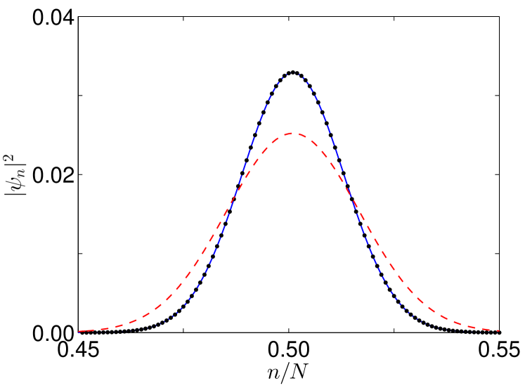
Figure 1: (Color online) Comparison of the exact ground state of the two-mode model (68) for $\alpha=0.95$ and $N=1000$ (dots) with the corresponding variational state (83) with optimal width parameter (85) (full line), and with the $N$-coherent state (80) (dashed). Plotted are the squares of the respective expansion coefficients $\psi_{n}$ in the Fock-state basis.

III.2 Equations of motion

The goal now is to explicitly carry through the construction process outlined in Sec. II, to monitor its accuracy, and to keep track of the errors committed, for the driven two-mode system (71). We are given the Schrödinger equation

$${\mathrm{i}}\hbar\frac{{\mathrm{d}}}{{\mathrm{d}}t}|\Psi(t)\rangle=H(t)|\Psi(t)\rangle$$ (87)

for $N$-particle Fock-space states $|\Psi(t)\rangle$ which are written without particle number index here, and we wish to construct mean-field amplitudes $c_{j}(t)$ such that

$$N|c_{j}(t)|^{2}=\langle\Psi(t)|a_{j}^{\dagger}a_{j}^{\phantom{\dagger}}|\Psi(t)\rangle$$ (88)

for $j=1,2$, in compliance with the central requirement (32). Starting from an initial $N$-particle state $|\Psi(t_{0})\rangle$ prepared at time $t=t_{0}$, we follow the prescription (33) and construct the two subsidiary $(N-1)$-particle states

$$|\widetilde{\Psi}_{j}(t_{0})\rangle:={\mathrm{e}}^{{\mathrm{i}}\gamma_{j}}\frac{a_{j}^{\phantom{\dagger}}|\Psi(t_{0})\rangle}{\|a_{j}^{\phantom{\dagger}}|\Psi(t_{0})\rangle\|}\;,$$ (89)

where the phases $\gamma_{j}$ can be chosen at will, and we are assuming that both sites are initially occupied, so that the denominators do not vanish. These states obviously permit the factorizations

$$\langle\Psi(t_{0})|a_{j}^{\dagger}a_{j}^{\phantom{\dagger}}|\Psi(t_{0})\rangle$$ (90)

$$= \langle\Psi(t_{0})|a_{j}^{\dagger}|\widetilde{\Psi}_{j}(t_{0})\rangle\langle\widetilde{\Psi}_{j}(t_{0})|a_{j}^{\phantom{\dagger}}|\Psi(t_{0})\rangle$$

and therefore allow one to define the candidate mean-field amplitudes at the initial moment:

$$\sqrt{N}c_{j}(t_{0}):=\langle\widetilde{\Psi}_{j}(t_{0})|a_{j}^{\phantom{\dagger}}|\Psi(t_{0})\rangle\;.$$ (91)

Then not only the actual initial state $|\Psi(t_{0})\rangle$ is subjected to the time evolution generated by $H(t)$, as expressed by the original Schrödinger equation (87), but also the two subsidiary states (89), giving rise to two further evolution equations

$${\mathrm{i}}\hbar\frac{{\mathrm{d}}}{{\mathrm{d}}t}|\widetilde{\Psi}_{j}(t)\rangle=H(t)|\widetilde{\Psi}_{j}(t)\rangle\;.$$ (92)

Here a decisive feature of the Fock-space formalism is exploited: Regardless of whether it acts on the $N$-particle sector or on the $(N-1)$-particle sector of Fock space, the Hamiltonian $H(t)$ is the same. Taking the solutions to these equations (87) and (92), the candidate mean-field amplitudes then are defined for all times $t\geq t_{0}$ in accordance with Eq. (40):

$$\sqrt{N}c_{j}(t):=\langle\widetilde{\Psi}_{j}(t)|a_{j}^{\phantom{\dagger}}|\Psi(t)\rangle\;.$$ (93)

Their equations of motion are obtained from the identity

$${\mathrm{i}}\hbar\frac{{\mathrm{d}}}{{\mathrm{d}}t}\langle\widetilde{\Psi}_{j}(t)|a_{j}^{\phantom{\dagger}}|\Psi(t)\rangle=\langle\widetilde{\Psi}_{j}(t)|\,\left[a_{j}^{\phantom{\dagger}},H(t)\right]\,|\Psi(t)\rangle\;.$$ (94)

Evaluating the commutator

$$\left[a_{1}^{\phantom{\dagger}},H(t)\right]=-\frac{\hbar\Omega}{2}a_{2}^{\phantom{\dagger}}+2\hbar\kappa a_{1}^{\dagger}a_{1}^{\phantom{\dagger}}a_{1}^{\phantom{\dagger}}+\hbar\mu(t)\sin(\omega t)a_{1}^{\phantom{\dagger}}$$ (95)

and taking the required matrix elements, one is led to

$${\mathrm{i}}\hbar\frac{{\mathrm{d}}}{{\mathrm{d}}t}\sqrt{N}c_{1}(t) = -\frac{\hbar\Omega}{2}\sqrt{N}c_{2}(t)f_{1}(t)$$ (96)

$$+2\hbar\kappa\langle\widetilde{\Psi}_{1}(t)|a_{1}^{\dagger}a_{1}^{\phantom{\dagger}}a_{1}^{\phantom{\dagger}}|\Psi(t)\rangle\phantom{\frac{\hbar\Omega}{2}}$$

$$+\hbar\mu(t)\sin(\omega t)\sqrt{N}c_{1}(t)\;,$$

where we have introduced the quantity

$$f_{1}(t)=\frac{\langle\widetilde{\Psi}_{1}(t)|a_{2}^{\phantom{\dagger}}|\Psi(t)\rangle}{\langle\widetilde{\Psi}_{2}(t)|a_{2}^{\phantom{\dagger}}|\Psi(t)\rangle}\;;$$ (97)

an analogous, still exact equation holds for $c_{2}(t)$. Observe the role of the ratio (97): When operating on Eq. (95) with $|\widetilde{\Psi}_{1}(t)\rangle$ from the left, and with $|\Psi(t)\rangle$ from the right, the tunneling term proportional to $a_{2}^{\phantom{\dagger}}$ yields its numerator, whereas the desired amplitude $c_{2}(t)$ is given by its denominator. Wilfully setting $f_{1}(t)\equiv 1$, and doing the same with the ratio $f_{2}(t)$ appearing in the equation for $c_{2}(t)$, corresponds to the uncontrolled step marked by “$\leadsto$” in the general Eq. (50); retaining both $f_{1}(t)$ and $f_{2}(t)$ in Eq. (96) and its $c_{2}(t)$-counterpart therefore renders these equations exact, and allows one to control one type of error accepted in the usual Gross-Pitaevskii approach. In the special case that the initial state $|\Psi(t_{0})\rangle$ is given by an atomic coherent state (78), the quasi-eigenvalue equations (79) ensure that $|\widetilde{\Psi}_{1}(t_{0})\rangle=|\widetilde{\Psi}_{2}(t_{0})\rangle=|\theta,\phi\rangle_{N-1}$, having set $\gamma_{1}=0$, $\gamma_{2}=-\phi$, and hence one deduces $|\widetilde{\Psi}_{1}(t)\rangle=|\widetilde{\Psi}_{2}(t)\rangle$ for all times $t\geq t_{0}$. Therefore, in this special case one actually has $f_{1}(t)=f_{2}(t)\equiv 1$, so that the above error does not occur. However, in all other cases it needs to be considered.

To proceed with Eq. (96), we now adapt the general steps (51) and (52) for processing the triple operator products:

$$\langle\widetilde{\Psi}_{j}(t)|a_{j}^{\dagger}a_{j}^{\phantom{\dagger}}a_{j}^{\phantom{\dagger}}|\Psi(t)\rangle$$ (98)

$$= \langle\widetilde{\Psi}_{j}(t)|\big{(}a_{j}^{\phantom{\dagger}}a_{j}^{\dagger}-1\big{)}a_{j}^{\phantom{\dagger}}|\Psi(t)\rangle$$

$$= \langle\widetilde{\Psi}_{j}(t)|a_{j}^{\phantom{\dagger}}a_{j}^{\dagger}a_{j}^{\phantom{\dagger}}|\Psi(t)\rangle-\sqrt{N}c_{j}(t)$$

$$\leadsto \langle\widetilde{\Psi}_{j}(t)|a_{j}^{\phantom{\dagger}}|\Psi(t)\rangle\langle\Psi(t)|a_{j}^{\dagger}|\widetilde{\Psi}_{j}(t)\rangle\langle\widetilde{\Psi}_{j}(t)|a_{j}^{\phantom{\dagger}}|\Psi(t)\rangle$$

$$-\sqrt{N}c_{j}(t)$$

$$= N^{3/2}c_{j}(t)\left(|c_{j}(t)|^{2}-\frac{1}{N}\right)\;.$$

The error introduced when assuming the factorization following the “$\leadsto$”-symbol is given by the difference

$$\Delta_{j}(t)=\langle\widetilde{\Psi}_{j}(t)|a_{j}^{\phantom{\dagger}}a_{j}^{\dagger}a_{j}^{\phantom{\dagger}}|\Psi(t)\rangle-N^{3/2}|c_{j}(t)|^{2}c_{j}(t)\;.$$ (99)

Hence, we have the exact evolution equation

$$\frac{{\mathrm{i}}}{\Omega}\frac{{\mathrm{d}}}{{\mathrm{d}}t}c_{1}(t) = -\frac{1}{2}c_{2}(t)f_{1}(t)$$ (100)

$$+2\frac{N\kappa}{\Omega}\left[\left(|c_{1}(t)|^{2}-\frac{1}{N}\right)c_{1}(t)+\frac{\Delta_{1}(t)}{N^{3/2}}\right]$$

$$+\frac{\mu(t)}{\Omega}\sin(\omega t)c_{1}(t)\;,$$

together with its counterpart for $c_{2}(t)$. Finally, taking the limit $N\to\infty$ such that

$$\frac{N\kappa}{\Omega}=\alpha={\rm const.}$$ (101)

we obtain the Gross-Pitaevskii equation for the driven two-mode system (71), with the proviso that both

$$f_{j}(t)\longrightarrow 1$$ (102)

and

$$\frac{\Delta_{j}(t)}{N^{3/2}}\longrightarrow 0$$ (103)

in this limit, for $j=1,2$: Again employing the dimensionless time variable $\tau=\Omega t$, we then have

$${\mathrm{i}}\frac{{\mathrm{d}}}{{\mathrm{d}}\tau}c_{1}(\tau) = -\frac{1}{2}c_{2}(\tau)+2\alpha|c_{1}(\tau)|^{2}c_{1}(\tau)$$

$$+ \frac{\mu(\tau)}{\Omega}\sin\left(\frac{\omega}{\Omega}\tau\right)c_{1}(\tau)\;,$$

$${\mathrm{i}}\frac{{\mathrm{d}}}{{\mathrm{d}}\tau}c_{2}(\tau) = -\frac{1}{2}c_{1}(\tau)+2\alpha|c_{2}(\tau)|^{2}c_{2}(\tau)$$ (104)

$$- \frac{\mu(\tau)}{\Omega}\sin\left(\frac{\omega}{\Omega}\tau\right)c_{2}(\tau)\;.$$

The key question, of course, is under what conditions the limits (102) and (103) actually are adopted, and how relevant these limits are when $N$ is still finite, and kept fixed.

A further question deriving from the discussion in Sec. II is to what extent the solution to this system (104) does comply with the basic requirement (88). In analogy with Eqs. (55) and (56) we now have the exact identities

$$\langle\Psi(t)|a_{j}^{\dagger}a_{j}^{\phantom{\dagger}}|\Psi(t)\rangle$$ (105)

$$= \langle\Psi(t)|a_{j}^{\dagger}|\widetilde{\Xi}_{j}(t)\rangle\langle\widetilde{\Xi}_{j}(t)|a_{j}^{\phantom{\dagger}}|\Psi(t)\rangle$$

with

$$|\widetilde{\Xi}_{j}(t)\rangle = \frac{a_{j}^{\phantom{\dagger}}|\Psi(t)\rangle}{\|a_{j}^{\phantom{\dagger}}|\Psi(t)\rangle\|}$$ (106)

$$= \frac{a_{j}^{\phantom{\dagger}}U(t,t_{0})|\Psi(t_{0})\rangle}{\|a_{j}^{\phantom{\dagger}}|\Psi(t)\rangle\|}\;,$$

whereas we require

$$\langle\Psi(t)|a_{j}^{\dagger}a_{j}^{\phantom{\dagger}}|\Psi(t)\rangle$$ (107)

$$= \langle\Psi(t)|a_{j}^{\dagger}|\widetilde{\Psi}_{j}(t)\rangle\langle\widetilde{\Psi}_{j}(t)|a_{j}^{\phantom{\dagger}}|\Psi(t)\rangle$$

with

$$|\widetilde{\Psi}_{j}(t)\rangle={\mathrm{e}}^{{\mathrm{i}}\gamma_{j}}\frac{U(t,t_{0})a_{j}^{\phantom{\dagger}}|\Psi(t_{0})\rangle}{\|a_{j}^{\phantom{\dagger}}|\Psi(t_{0})\rangle\|}\;.$$ (108)

The actually fulfilled Eq. (105) is compatible with the desired Eq. (107) if $|\widetilde{\Xi}_{j}(t)\rangle$ differs from $|\widetilde{\Psi}_{j}(t)\rangle$ merely by a phase factor, demanding a relation

$$a_{j}^{\phantom{\dagger}}|\Psi(t)\rangle=\eta_{j}(t)|\widetilde{\Psi}_{j}(t)\rangle\;;$$ (109)

the definition (93) of the candidate mean-field amplitude then immediately yields

$$\eta_{j}(t)=\sqrt{N}c_{j}(t)\;.$$ (110)

Thus, we are led to a set of two consistency equations analogous to Eq. (64) which embody the property of perfect $t$-coherence:

$$a_{j}^{\phantom{\dagger}}|\Psi(t)\rangle=\sqrt{N}c_{j}(t)|\widetilde{\Psi}_{j}(t)\rangle\;;$$ (111)

this is the property which guarantees the validity of the basic Eq. (88) underlying the entire construction process.

Following Eq. (II), the degree to which $t$-coherence actually does prevail, that is, the stiffness of Fock-space flow in the vicinity of the initial state, is quantified by the scalar products

$$R_{j}(t) = {\mathrm{e}}^{{\mathrm{i}}\gamma_{j}}\langle\widetilde{\Psi}_{j}(t)|\widetilde{\Xi}_{j}(t)\rangle$$ (112)

$$= {\mathrm{e}}^{{\mathrm{i}}\gamma_{j}}\frac{\langle\widetilde{\Psi}_{j}(t)|a_{j}^{\phantom{\dagger}}|\Psi(t)\rangle}{\|a_{j}^{\phantom{\dagger}}|\Psi(t)\rangle\|}$$

$$= \frac{\langle\Psi(t_{0})|a_{j}^{\dagger}U^{\dagger}(t,t_{0})a_{j}^{\phantom{\dagger}}U(t,t_{0})|\Psi(t_{0})\rangle}{\|a_{j}^{\phantom{\dagger}}|\Psi(t_{0})\rangle\|\;\|a_{j}^{\phantom{\dagger}}|\Psi(t)\rangle\|}\;.$$

If both $|\widetilde{\Xi}_{j}(t)\rangle$ and $|\widetilde{\Psi}_{j}(t)\rangle$ represent the same ray in Fock space, as is implied by the consistency condition (111), then $|R_{j}(t)|=1$; monitoring the absolute value of this scalar product (112) therefore allows one to assess, on the basis of the exact $N$-particle solutions $|\Psi(t)\rangle$ and the $(N-1)$-particle solutions $|\widetilde{\Psi}_{j}(t)\rangle$, the possible accuracy of a Gross-Pitaevskii-treatment. Moreover, if close-to-perfect $t$-coherence is given and Eq. (111) is satisfied more or less exactly, then one has

$$R_{j}(t)={\mathrm{e}}^{{\mathrm{i}}\gamma_{j}}\frac{c_{j}(t)}{|c_{j}(t)|}\;,$$ (113)

so that the phase of $R_{j}(t)$ equals the phase of the respective mean-field amplitude, up to $\gamma_{j}$. Read in the reverse direction, this means that if a Gross-Pitaevskii approach is viable, then the phase of the easily obtainable mean-field amplitudes contains valuable information about the exact many-particle dynamics, more precisely, on the difference between the evolution of $N$ and $(N-1)$ particles.

III.3 Numerical studies

Since the dynamics of the driven Josephson junction (71), when occupied with $N$ particles, takes place in a merely $(N+1)$-dimensional complex Hilbert space, solving the equations of motion for moderately large $N$ does not pose severe computational difficulties. For ensuring high numerical accuracy we employ a variable-order Adams PECE algorithm, of the type originally elaborated by Shampine and Gordon ShampineGordon75 , routinely reaching particle numbers $N$ on the order of a few thousand.

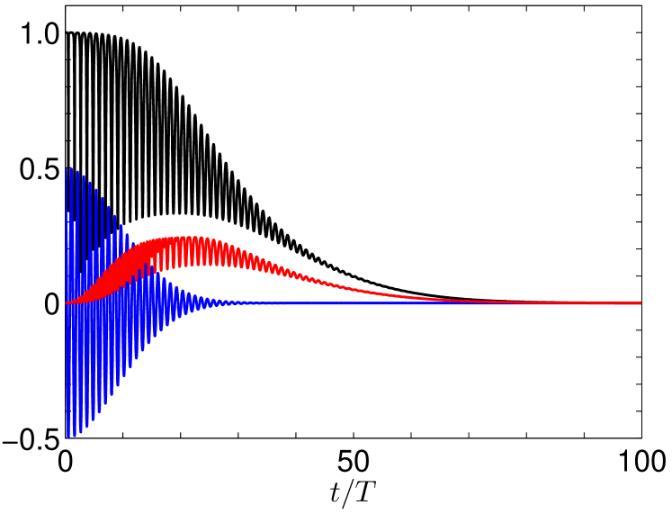
Figure 2: (Color online) Scaled population imbalance $\langle J_{z}\rangle/N$ (blue line), closure error $|\Delta_{1}|/N^{3/2}$ (red line), and stiffness $|R_{1}|$ (black line) for the undriven Josephson junction (68) with $\alpha=0.5$ and $N=1000$. The initial state is the Fock state $|N,0\rangle$, which is $N$-coherent. Here and in the following figures, time $t$ is measured in multiples of $T=2\pi/\Omega$.

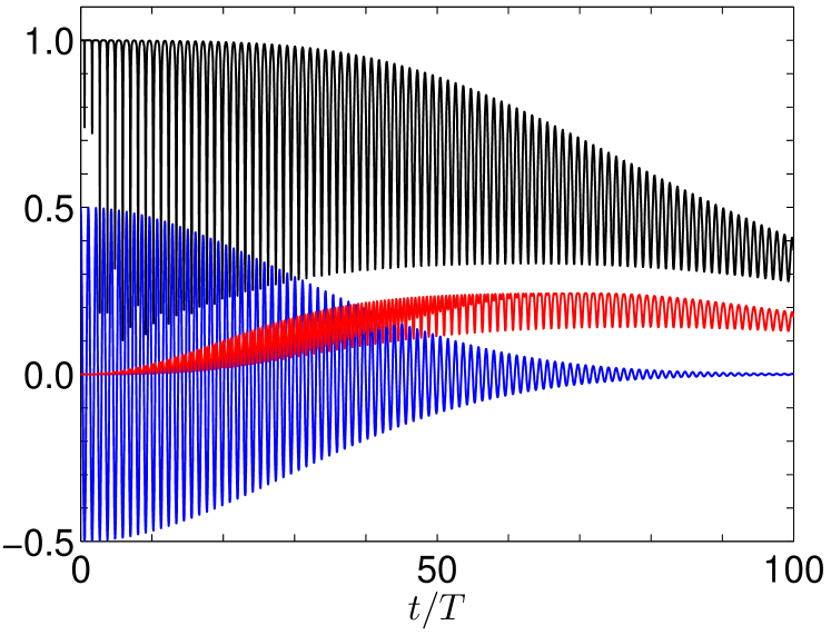
Figure 3: (Color online) As Fig. 2, but with $N=10000$.

The diagnostic tools now at our disposal are the ratios (97), the errors of closure (99), and the stiffnesses (112). While the first and the second of these tools allow one to trace sources of deviations from Gross-Pitaevskii behavior, the third one evaluates the degree of $t$-coherence of the evolving many-body wave function, admitting a truthful Gross-Pitaevskii description only when $|R_{j}(t)|=1$.

As preliminary examples for the performance of these tools we monitor the dynamics of the junction (68) in the absence of the drive (72). As initial condition we select $|\Psi(0)\rangle=|N,0\rangle$, so that all particles occupy site 1 at $t_{0}=0$. Then $|\widetilde{\Psi}_{1}(0)\rangle=|N-1,0\rangle$ is given by Eq. (89), with $\gamma_{1}=0$. Moreover, since the initial Fock state $|N,0\rangle$ equals an $N$-coherent state (78) with $\theta=0$ and arbitrary $\phi$, we may set $|\widetilde{\Psi}_{2}(t)\rangle=|\widetilde{\Psi}_{1}(t)\rangle$ for $t\geq 0$. This implies $f_{1}(t)=f_{2}(t)\equiv 1$, so that all deviations from mean-field dynamics are solely due to the closure errors. Figure 2 depicts the scaled population imbalance

$$\langle J_{z}\rangle(t)/N=\langle\Psi(t)|a_{1}^{\dagger}a_{1}^{\phantom{\dagger}}-a_{2}^{\dagger}a_{2}^{\phantom{\dagger}}|\Psi(t)\rangle/(2N)$$ (114)

for $N=1000$ and scaled interaction strength $\alpha=0.5$, together with the scaled error of closure $|\Delta_{1}(t)|/N^{3/2}$ and the stiffness $|R_{1}(t)|$, with time $t$ being measured in multiples of $T=2\pi/\Omega$. The quantities $|\Delta_{2}(t)|/N^{3/2}$ and $|R_{2}(t)|$ behave quite similar to their respective counterparts. One observes the familiar collapse of the oscillating population imbalance, caused by dephasing due to the finite particle number, which is to be followed by revivals at later times, when the components of the wave function rephase SimonStrunz12 ; HolthausStenholm01 ; WrightEtAl96 ; LewensteinYou96 . The most significant error of closure occurs during the collapse stage, leading to a stiffness which decreases to zero in an oscillating manner. When increasing the particle number to $N=10000$, while keeping $\alpha=0.5$ fixed so that, in accordance with Eq. (101), the interparticle interaction strength $\hbar\kappa$ is reduced by a factor of $10$, the collapse proceeds more slowly, as plotted in Fig. 3. The comparison of the $N$-particle dynamics for both $N=1000$ and $N=10000$ with the prediction

$$\langle J_{z}\rangle_{\rm mf}(t)=\Big{(}|c_{1}(t)|^{2}-|c_{2}(t)|^{2}\Big{)}/2$$ (115)

of the Gross-Piaevskii equation (69) displayed in Fig. 4 provides convincing evidence for convergence in the limit $N\to\infty$, when $\alpha$ is held constant: Given any moment $t_{1}>0$, the particle number $N$ can be increased such that the true populations of the two sites, calculated from the $N$-particle Schrödinger equation, differ by an arbitrary small amount from the corresponding mean-field data in the entire interval from $t_{0}=0$ to $t_{1}$ in the example considered here. But as pointed out in Sec. III.1, this situation is exceptionally simple insofar as the mean-field equation of motion (69) is integrable.

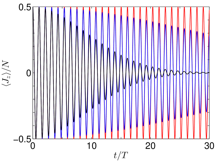
Figure 4: (Color online) Scaled population imbalance $\langle J_{z}\rangle/N$ for the undriven Josephson junction (68) with $\alpha=0.5$ for $N=1000$ (black line) and $N=10000$ (blue line), in comparison with the prediction of the Gross-Pitaevskii equation (69) (red line). In each case, all particles are initially located at site 1.

For assessing the conceptually far more difficult, but generic cases of non-integrable mean-field dynamics we now turn to the driven Josephson junction (71), and choose a Gaussian envelope function

$$\mu(t)=\mu_{\rm max}\exp\left(-\frac{t^{2}}{2\sigma^{2}}\right)\;,$$ (116)

so that the drive (72) models a single pulse with maximum amplitude $\hbar\mu_{\rm max}$, carrier frequency $\omega$, and width $\sigma$. For all following calculations we set $\omega/\Omega=1.0$ and $\sigma/T=10.0$, where again $T=2\pi/\Omega$. Thus, the driving frequency is at resonance with the single-particle tunneling frequency, and the driving amplitude increases smoothly from almost zero to its maximum within about $30$ driving cycles, then decreasing within another $30$ cycles.

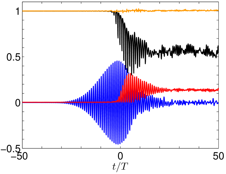
Figure 5: (Color online) Dynamics of the driven Josephson junction (71) with $\alpha=0.95$ and $N=100$ under the influence of a Gaussian pulse (116) with maximum amplitude $\mu_{\rm{max}}/\Omega=0.9$, scaled frequency $\omega/\Omega=1.0$, and width $\sigma/T=10.0$. Shown are the scaled population imbalance $\langle J_{z}\rangle/N$ (blue line), the closure error $|\Delta_{1}|/N^{3/2}$ (red line), the real part ${\rm Re}(f_{1})$ of the ratio (97) (orange line), and the stiffness $|R_{1}|$ (black line). The initial state is the ground state of the undriven junction (68).

As initial condition for large negative times we now select the ground state of the undriven junction (68), which, according to Sec. III.1, differs from an $N$-coherent state even for arbitrarily large $N$. Hence, now $|\widetilde{\Psi}_{2}(t)\rangle$ is different from $|\widetilde{\Psi}_{1}(t)\rangle$, and we have to keep track of the ratios (97). Figure 5 shows the dynamics for $\alpha=0.95$ and comparatively small particle number $N=100$ in response to a pulse with maximum scaled amplitude $\mu_{\rm max}/\Omega=0.9$. Here the error of closure remains fairly small until a few cycles before the pulse’s envelope reaches its maximum. During that same interval one finds both $f_{1}(t)\approx 1$ and $f_{2}(t)\approx 1$ to good accuracy, and, most importantly, both stiffnesses $|R_{1}(t)|$ and $|R_{2}(t)|$ remain close to unity before they drop to values fluctuating around about $0.5$ in the second half of the pulse. This diagnosis forecasts that the Gross-Pitaevskii equation will describe the pulsed $N$-particle dynamics quite faithfully until about the pulse’s maximum, and then become unreliable. This prediction is fully borne out by Fig. 6, which compares the true population imbalance (114) for this pulse to the mean-field imbalance (115), as computed from Eq. (104): As long as $|R_{j}(t)|\approx 1$, the simple Gross-Pitaevskii equation does a remarkably good job.

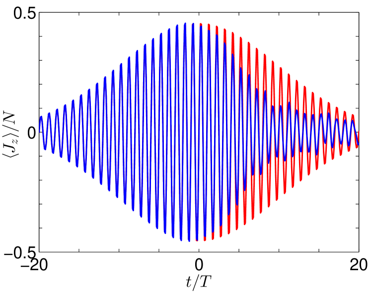
Figure 6: (Color online) Comparison of the population imbalance for $N=100$ under the action of the pulse monitored in Fig. 5 (blue line) to the corresponding prediction of the Gross-Pitaevskii equation (104) (red line).

Figure 7: (Color online) As Fig. 5, but with $N=1000$.

A far more impressive example for the possible accuracy of the Gross-Pitaevskii equation is given in Fig. 7: Here the particle number has been increased from $N=100$ to $N=1000$, while all other parameters are the same as in Fig. 5, again implying a reduction of the interaction strength $\hbar\kappa$ so as to keep $\alpha$ constant. Throughout this pulse the closure error remains negligible, and both ratios $f_{j}(t)$ stay close to unity, as witnessed on a fine scale by Fig. 8. This results in almost perfect $t$-coherence of the evolution, even though the initial state is not fully $N$-coherent, guaranteeing excellent mean-field approximability of the entire pulse dynamics. Since the maximum scaled amplitude $\mu_{\rm max}/\Omega=0.9$ is by no means small, as is evident from the quite significant response of the population imbalance, this finding is far from trivial.

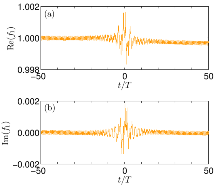
Figure 8: (Color online) Real and imaginary part of the ratio $f_{1}$ for the pulse monitored in Fig. 7.

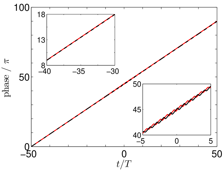
Figure 9: (Color online) Comparison of the phase of the mean-field amplitude $c_{1}(t)$ (red line) with that of $R_{1}(t)$ (black) for the pulse monitored in Fig. 7, for which $|R_{1}(t)|=1$ to good accuracy. The insets magnify the evolution of the phases at the beginning of the pulse, and around its maximum, where in view of Fig. 8 the mean-field approximation is most critical. At the end of the pulse, the phases differ by $0.210\,\pi$.

According to Eq. (113) the phase of the scalar product $R_{j}(t)$ should determine the phase of the mean-field amplitude $c_{j}(t)$ in case of perfect $t$-coherence, when $|R_{j}(t)|=1$. This is confirmed in Fig. 9 for the pulse studied in Fig. 7, which meets the above requirement to good accuracy: With $\gamma_{1}=0$, the phase of $c_{1}(t)$ practically coincides with that of $R_{1}(t)$, growing linearly with time.

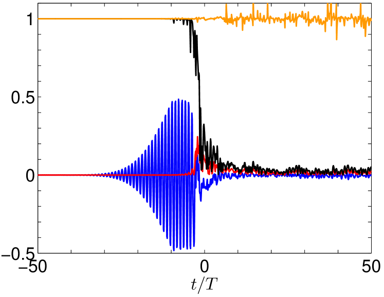
Figure 10: (Color online) As Fig. 5, but with $N=1000$ and $\mu_{\rm{max}}/\Omega=1.5$.

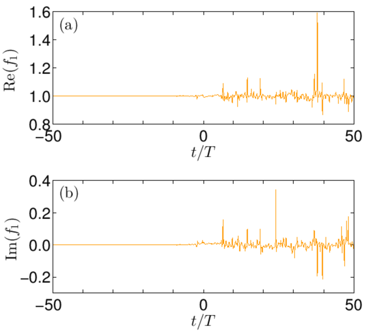
Figure 11: (Color online) Real and imaginary part of the ratio $f_{1}$ for the pulse monitored in Fig. 10. Observe the change of the ordinates’ scale in comparison with Fig. 8!

An opposite paradigm is captured by Fig. 10, again for $N=1000$, but now the maximum scaled amplitude has been increased to $\mu_{\rm max}/\Omega=1.5$. Here the response of the $N$-particle system is characterized by a stiffness which remains close to perfect almost up to the pulse’s maximum, but then rapidly drops to values close to zero, as a consequence of a suddenly emerging error of closure, and of the sudden change of behavior exhibited by the ratios $f_{j}(t)$ which is detailed in Fig. 11. These errors drive the solution to the Gross-Pitaevskii equation (104) off its intended track, to such an extent that any tangible connection to the actual $N$-particle dynamics appears to be lost.

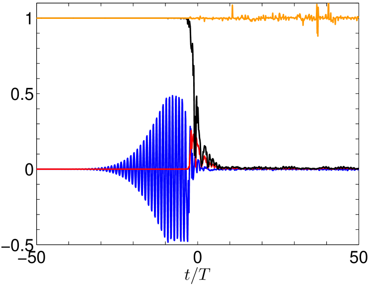
Figure 12: (Color online) As Fig. 5, but with $N=10000$ and $\mu_{\rm{max}}/\Omega=1.5$, confirming the “sudden death” of the mean field already observed in Fig. 10.

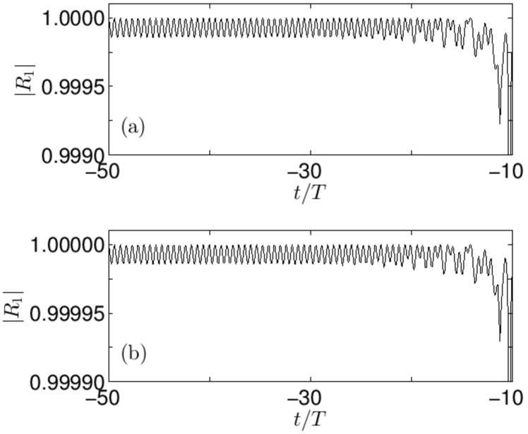
Figure 13: Stiffness $|R_{1}(t)|$ during the rise of the pulses monitored in Fig. 10, where $N=1000$ (a), and in Fig. 12, where $N=10000$ (b). Observe the scaling with the particle number.

One might hope that, similar to the effect achieved when going from $N=100$ in Fig. 5 to $N=1000$ in Fig. 7, the loss of $t$-coherence recorded in Fig. 10 could be counteracted by increasing the particle number still further. However, this is not the case: Figure 12 illustrates the system’s response when $N=10000$, with all other parameters equaling those employed in Fig. 10. While Fig. 13 testifies that now the stiffness deviates from unity by not more than $2\times 10^{-5}$ during the rise of the pulse, apparently scaling with $1/N$, it then drops even more sharply, indicating a “sudden death” of the mean field, i.e., a dynamically induced sudden loss of $t$-coherence, as corresponding to a sudden destruction of the macroscopic wave function GertjerenkenHolthaus15 . With the help of the following semiclassical deliberations we will argue that this loss of $t$-coherence persists in the formal limit $N\to\infty$, when $\alpha$ is kept constant: In the situation scrutinized in Figs. 10 and 12 there is no chance to describe the system’s time evolution correctly by means of the Gross-Pitaevskii equation, not even for arbitrarily large particle numbers.

III.4 Semiclassical interpretation

We now exploit the circumstance that the dynamics generated by the time-dependent Gross-Pitaevskii equation (104) are equivalent to those of a driven nonlinear pendulum RaghavanEtAl99 ; HolthausStenholm01 . Starting from the polar representation

$$c_{j}=|c_{j}|{\mathrm{e}}^{{\mathrm{i}}\vartheta_{j}}$$ (117)

of the mean-field amplitudes, and introducing their imbalance

$$z=|c_{1}|^{2}-|c_{2}|^{2}$$ (118)

and the relative phase

$$\phi=\vartheta_{2}-\vartheta_{1},$$ (119)

the equation of motion (104) readily yields

$${\mathrm{i}}\frac{{\mathrm{d}}z}{{\mathrm{d}}\tau} = c_{1}c_{2}^{*}-c_{1}^{*}c_{2}$$ (120)

$$= -|c_{1}||c_{2}|\left({\mathrm{e}}^{{\mathrm{i}}\phi}-{\mathrm{e}}^{-{\mathrm{i}}\phi}\right)\;.$$

Observing

$$1-z^{2}=4|c_{1}|^{2}|c_{2}|^{2}\;,$$ (121)

this becomes

$$\frac{{\mathrm{d}}z}{{\mathrm{d}}\tau}=-\sqrt{1-z^{2}}\sin\phi\;.$$ (122)

Similarly, one has

$$c_{1}c_{2}^{*}+c_{1}^{*}c_{2}=\sqrt{1-z^{2}}\cos\phi\;,$$ (123)

giving

$$\frac{{\mathrm{d}}}{{\mathrm{d}}\tau}\left(c_{1}c_{2}^{*}+c_{1}^{*}c_{2}\right)=z\sin\phi\cos\phi-\sqrt{1-z^{2}}\sin\phi\frac{{\mathrm{d}}\phi}{{\mathrm{d}}\tau}\;,$$ (124)

where Eq. (122) has been used. On the other hand, one deduces

$${\mathrm{i}}\frac{{\mathrm{d}}}{{\mathrm{d}}\tau}\left(c_{1}c_{2}^{*}+c_{1}^{*}c_{2}\right)$$ (125)

$$= 2\Big{[}\alpha\left(|c_{1}|^{2}-|c_{2}|^{2}\right)+f(\tau)\Big{]}\left(c_{1}c_{2}^{*}-c_{1}^{*}c_{2}\right)$$

from the Gross-Pitaevskii equation (104), having written

$$f(\tau)=\frac{\mu(\tau)}{\Omega}\sin\left(\frac{\omega}{\Omega}\tau\right)\;,$$ (126)

so that

$$\frac{{\mathrm{d}}}{{\mathrm{d}}\tau}\left(c_{1}c_{2}^{*}+c_{1}^{*}c_{2}\right)=-2\Big{[}\alpha z+f(\tau)\Big{]}\sqrt{1-z^{2}}\sin\phi\;.$$ (127)

Combining Eqs. (124) and (127) then leads to

$$\frac{{\mathrm{d}}\phi}{{\mathrm{d}}\tau}=2\alpha z+\frac{z}{\sqrt{1-z^{2}}}\cos\phi+2f(\tau)\;.$$ (128)

These equations of motion (122) and (128) for the mean-field imbalance and the relative phase constitute a pair of Hamiltonian equations derived from the classical Hamiltonian function

$$H_{\rm nlp}(z,\phi,\tau)=\alpha z^{2}-\sqrt{1-z^{2}}\cos\phi+2zf(\tau)$$ (129)

in which $z$ plays the role of a momentum variable, and $\phi$ that of its canonically conjugate coordinate, and which can thus be interpreted as the Hamiltonian of a nonlinear pendulum with mass propotional to $1/\alpha$, and with momentum-dependent length, which is driven by the external force $f(\tau)$: Evidently, one has

$$\frac{{\mathrm{d}}\phi}{{\mathrm{d}}\tau}=\frac{\partial H_{\rm nlp}}{\partial z}\quad,\quad\frac{{\mathrm{d}}z}{{\mathrm{d}}\tau}=-\frac{\partial H_{\rm nlp}}{\partial\phi}\;.$$ (130)

In passing, we remark that for $|z|\ll 1$ this pair reduces to

$$\frac{{\mathrm{d}}\phi}{{\mathrm{d}}\tau} \approx 2f(\tau)$$

$$\frac{{\mathrm{d}}z}{{\mathrm{d}}\tau} \approx -\sin\phi\;,$$ (131)

as corresponding to the equations for the phase and the current across a macroscopic superconducting Josephson junction BaronePaterno82 .

This classical viewpoint underlines the significance of the extension of the Lipkin-Meshkov-Glick model (68) by the time-dependent drive (72): When $f(\tau)=0$, the Hamiltonian (129) represents a dynamical system with one single degree of freedom, possessing energy as its integral of motion. Adding a time-dependent force is tantamount to adding a further degree of freedom not accompanied, in general, by a further integral of motion, so that the driven nonlinear pendulum is non-integrable in the sense of classical Hamiltonian mechanics Gutzwiller90 ; JoseSaletan98 , giving rise to chaotic motion. This raises the question how the actual, linear $N$-particle system behaves when its nonlinear mean-field descendant becomes chaotic.

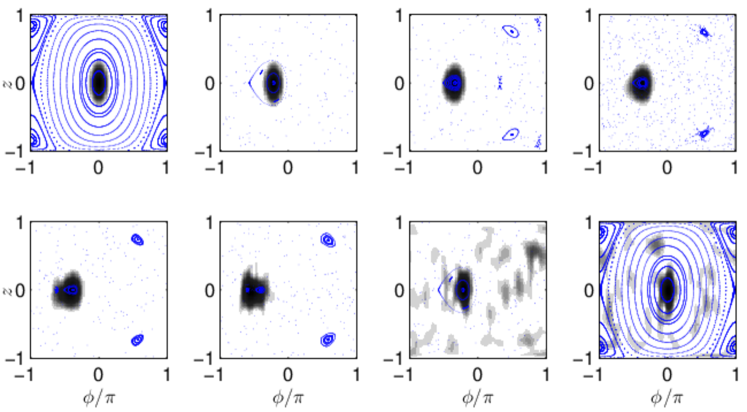
Figure 14: (Color online) Grey-scale Husimi snapshots of the evolving $N$-particle state for the pulse monitored in Fig. 5, for which $N=100$ and $\mu_{\rm max}/\Omega=0.9$, superimposed onto the instantaneous Poincaré surfaces of section (blue) at successive times $t$ when $\mu(t)/\Omega=0.0$, $0.6$, $0.83$, $0.86$, $0.88$, $0.9$, $0.6$, $0.0$ (upper left to lower right). Here the quantum state initially remains associated with an adiabatic invariant corresponding to a closed curve in the regular island, as selected by the Bohr-Sommerfeld condition (135) with $n=0$, but then spreads over the stochastic sea when the island becomes so small that the invariant is destroyed.

A useful link between the $N$-particle level and its mean-field description in terms of the Hamiltonian system (130) is provided by the $SU(2)$-coherent states (78): Taking the expectation value of the $N$-particle Hamiltonian (71) with respect to these states, one obtains

$$\frac{{{}_{N}\langle}\theta,\phi|H(t)|\theta,\phi\rangle_{N}}{N\hbar\Omega/2}$$ (132)

$$= \alpha\left(1-\frac{1}{N}\right)\left(\cos^{2}\theta+1\right)-\sqrt{1-\cos^{2}\theta}\cos\phi$$

$$+2\cos\theta\;\frac{\mu(t)}{\Omega}\sin(\omega t)\;,$$

which equals the classical Hamiltonian (129) up to an irrelevant constant if one neglects terms of order ${\mathcal{O}}(1/N)$, and sets

$$z=\cos\theta\;.$$ (133)

Since $\cos\theta=\cos^{2}(\theta/2)-\sin^{2}(\theta/2)$, this is in perfect correspondence with the representation (76) of the $N$-fold occupied single-particle state which underlies the $N$-coherent state $|\theta,\phi\rangle_{N}$ on the one hand, and with the definition (118) on the other. Therefore, the squared projections

$$\mathcal{Q}_{N}(z,\phi,t)=\big{|}{{}_{N}\langle}\theta,\phi|\Psi(t)\rangle\big{|}^{2}\;,$$ (134)

referred to as Husimi distributions, quantify the degree of affinity of the $N$-particle state $|\Psi(t)\rangle$ with the phase-space point $(z,\varphi)$ at the moment $t$ WeissTeichmann08 ; GraefeEtAl14 ; GertjerenkenHolthaus14 . This observation leads to the desired semiclassical view on the pulse dynamics recorded in Sec. III.3: We take the solution $|\Psi(t)\rangle$ to the $N$-particle Schrödinger equation at certain moments $t$, compute the associated Husimi distributions (134), and superimpose these distributions onto the corresponding classical phase-space portraits, that is, onto the Poincaré surfaces of section of the accompanying pendulum which is periodically driven with amplitude $\mu/\Omega$ “frozen” at the value reached at the moment $t$ under study. These surfaces of section are computed by solving the classical equations of motion for a representative set of initial conditions with fixed driving amplitude $\mu/\Omega$, and by plotting the resulting phase-space points stroboscopically after each driving period $2\pi/\omega$.

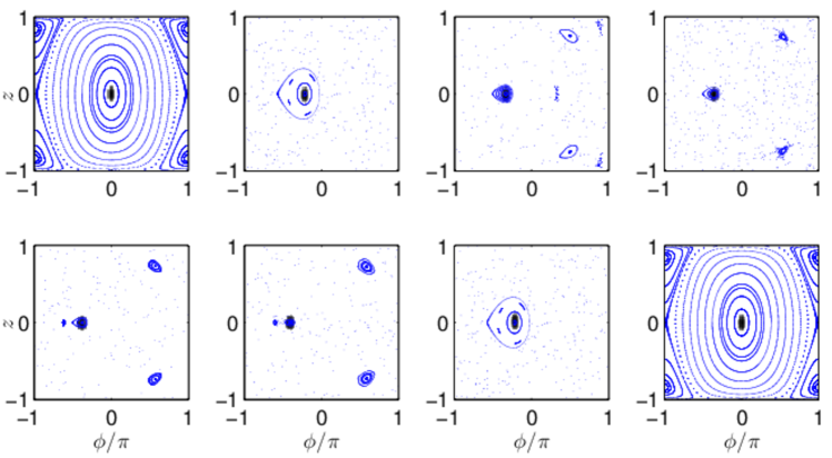
Figure 15: (Color online) Grey-scale Husimi snapshots of the evolving $N$-particle state for the pulse monitored in Fig. 7, for which $N=1000$ and $\mu_{\rm max}/\Omega=0.9$, superimposed onto the instantaneous Poincaré surfaces of section (blue) at successive times $t$ when $\mu(t)/\Omega=0.0$, $0.6$, $0.83$, $0.86$, $0.88$, $0.9$, $0.6$, $0.0$ (upper left to lower right). While the Poincaré sections are the same as those displayed in Fig. 14, now the curve $\gamma_{0}$ required by the Bohr-Sommerfeld condition (135) encircles an area which is reduced by a factor of $10$, and thus remains confined in the regular island during the entire pulse, enabling adiabatic following of the $N$-particle quantum state.

Figure 14 shows a series of snapshots obtained in this manner for the pulse previously studied in Fig. 5, for which $N=100$ and $\mu_{\rm max}/\Omega=0.9$. Initially, when $\mu/\Omega=0$, the accompanying classical pendulum is integrable, as is reflected by a phase-space portrait which is stratified into closed curves remaining invariant under the Hamiltonian flow. The initial quantum state considered here, which is the ground state of the undriven system (68) as depicted in Fig. 1, is semiclassically linked by means of the WKB-construction to that invariant curve $\gamma_{n}$ surrounding the central fixed point which is selected by the Bohr-Sommerfeld condition NissenKeeling10 ; SimonStrunz12 ; GraefeEtAl14 ; GertjerenkenHolthaus14

$$\frac{1}{2\pi}\oint_{\gamma_{n}}\!z\mathrm{d}\phi=\hbar_{\rm eff}\left(n+\frac{1}{2}\right)$$ (135)

with effective Planck constant

$$\hbar_{\rm eff}=\frac{2}{N}\;,$$ (136)

and with quantum number $n=0$, so that its Husimi distribution appears concentrated around that curve $\gamma_{0}$. When the driving amplitude is increased, a large fraction of the invariant curves is destroyed giving way to chaotic motion, while those surrounding the central fixed point are deformed, but remain preserved if $\mu/\Omega$ does not become too large, forming a regular island embedded in a chaotic sea. If the pulse’s amplitude increases on a time scale which is slow compared to the period $2\pi/\omega$, these preserved curves represent adiabatic invariants to which the time-evolving wave function remains tied in a WKB-type manner. This is what explains the scenario depicted in Fig. 14: For low driving strength the evolving quantum state clinges to its adiabatic invariant still contained in the regular island, but with increasing amplitude the island becomes so small that the required invariant does no longer exist. Then the Husimi projection of the quantum state, having nothing left it can cling to, spills out more or less over the entire phase space, leading to a final quantum state which contains many eigenstates of the undriven junction (68).

With this background knowledge the difference between the pulses recorded in Fig. 5 on the one hand, and in Fig. 7 on the other, becomes intuitively clear, recalling that for the latter pulse the maximum scaled amplitude $\mu_{\rm max}/\Omega=0.9$ has been maintained while the particle number has been increased to $N=1000$. Because this implies that the effective Planck constant (136) is reduced by a factor of $10$, the required phase-space curve $\gamma_{0}$ now encircles a correspondingly smaller area. As shown in Fig. 15, it therefore fits into the shrinking and re-growing regular island during the entire pulse, albeit just barely so at its maximum. Thus, the quantum state evolving under the influence of the pulse remains semiclassically associated with an adiabatic invariant which is preserved from the pulse’s beginning until its end, and thus enables adiabatic following. As a result, the final $N$-particle state here closely resembles the initial one.

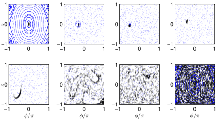
Figure 16: (Color online) Grey-scale Husimi snapshots of the evolving $N$-particle state for the pulse monitored in Fig. 10, for which $N=1000$ and $\mu_{\rm max}/\Omega=1.5$, superimposed onto the instantaneous Poincaré surfaces of section (blue) at successive times $t$ when $\mu(t)/\Omega=0.0$, $0.73$, $1.0$, $1.25$, $1.43$, $1.5$, $1.43$, $0.0$ (upper left to lower right). Here the regular island is completely destroyed in the middle of the pulse, implying that there is no adiabatic invariant capable of carrying a macroscopic wave function. Thus, even for arbitrarily large particle number the state becomes so complex that a Gross-Pitaevskii description is impossible.

A mere glimpse on Fig. 16 then suffices to grasp why no further enhancement of the particle number whatsoever, together with the implied reduction of the interparticle interaction in order to maintain a constant value of $\alpha$, could possibly bring one back to the Gross-Pitaevskii regime under the conditions of Figs. 10 and 12: Here the pulse possesses the maximum amplitude $\mu_{\rm max}/\Omega=1.5$, which is so strong that the regular island which still hosts the adiabatic invariant at the early stages of the pulse is destroyed completely when the envelope approaches its maximum. Hence, no matter how large the particle number $N$ and, consequently, how small the effective Planck constant (136), there is no preserved adiabatic invariant which could possibly carry a macroscopic wave function. Instead, Fig. 16 visualizes that upon destruction of the island the quantum state aquires a degree of complexity which strikingly contrasts the simplicity of the initial condition. Obviously this sudden increase of complexity, as corresponding to a sudden loss of order, reflects the sudden drop of stiffness observed in Figs. 10 and 12, signaling the sudden death of the mean field. We suggest that this scenario is quite general, so that it would be experimentally accessible, for instance, with pulsed Bose-Einstein condensates in anharmonic trapping potentials GertjerenkenHolthaus15 .

IV Discussion

One usually takes recourse to a mean-field theory, which in many cases is still tractable by numerical means, to obtain information on intricate many-particle dynamics, which in general do not lend themselves to direct simulations. In our approach to the time-dependent Gross-Pitaevskii equation this common strategy has been reversed, in order to clarify questions concerning the emergence and possible persistence of an order parameter in a system of $N$ Bosons exposed to external forcing: Assuming that we know its exact many-particle wave function $\Psi(\bm{r}_{1},\ldots,\bm{r}_{N};t)$, we have asked how this knowledge can be used for constructing the associated macroscopic wave function, provided that it exists, in the form of a mean-field amplitude $\Phi(\bm{r};t)$. The answer, formalized in Eqs. (33), (38), (39), and (40), is conceptually interesting insofar as it does neither involve the formal limit $N\to\infty$, nor the notion of spontaneous symmetry breaking: Take the initial $N$-particle state, annihilate a particle, and propagate both the initial state and the subsidiary $(N-1)$-particle states thus obtained in time; a candidate mean-field amplitude then is introduced by taking the matrix elements of the annihilation operator with these evolving states.

The starting point of this construction resembles the specification of a condensate wave function by Lifshitz and Pitaevskii LaLifIX , but the additional consideration of time evolution in response to external forcing brings about a new twist. Namely, in order to decide whether or not the candidate actually is a proper mean-field amplitude, which is tantamount to the question whether or not a macroscopic wave function of the driven system still does exist, it is not sufficient to follow solely the trajectory of the given $N$-particle state in Fock space. Rather, one has to compare this given trajectory to other trajectories initially close to it, differing by one in particle number, and to check to what extent these initially close trajectories diverge in the course of time. This is what is effectively quantified by the projection (II): If the absolute value of this scalar product $R(\bm{r};t)$ equals unity to good approximation, the state obtained by first evolving the initial condition in time and annihilating a particle at a later moment differs merely by a phase factor from the states obtained by annihilating first and evolving thereafter. This property of $t$-coherence, indicated by $|R(\bm{r};t)|=1$, means that initial states differing by one in particle number move in some sense parallel to each other in Fock space. In this case the flow in Fock space can be considered as stiff, similar to laminar flow in fluid mechanics. This is the quality of “simplicity” required for ensuring the presence of a genuine mean-field amplitude: If $|R(\bm{r};t)|=1$ at least to a good approximation, the candidate actually qualifies as a macroscopic wave function and obeys the time-dependent Gross-Pitaevskii-equation; if not, it has no immediate physical significance.

The model of the driven Josephson junction studied in Sec. III suggests that the occurrence of chaotic solutions to the Gross-Pitaevskii equation reflects the loss of $t$-coherence on the $N$-particle level. Our findings thus extend previous studies CastinDum97 ; GardinerEtAl00 ; BrezinovaEtAl11 ; BrezinovaEtAl12 which have cast doubt on the validity of a Gross-Pitaevskii-type mean-field approach under chaotic conditions. It appears that the distinction between order and chaos, which has been explored in great depth in classical mechanics Gutzwiller90 ; JoseSaletan98 , may have implications of its own in quantum many-body physics. In particular, the scenario depicted in Fig. 12 indicates in a striking manner that a macroscopic wave function can be destroyed almost instantaneously upon entering a chaotic regime.

Recent pioneering works which have taken up the investigation of many-body quantum chaos have considered $\delta$-kicked condensates ZhangEtAl04 ; LiuEtAl06 ; DuffyEtAl04 ; WimbergerEtAl05 ; BillamGardiner12 ; BillamEtAl13 . In contrast, here we have studied the response to a sinusoidal force with a “slowly” varying envelope. One of our most important results, albeit obtained for one particular model system only, consists in the observation that adiabatic following to such slowly changing driving forces allows one to preserve a pre-existing macroscopic wave function, and to transport it almost without loss of $t$-coherence into the regime of strong driving, as shown exemplarily in Fig. 7. This finding almost provides a blueprint for generating Floquet condensates GertjerenkenHolthaus14 . More generally, it may be of interest for guiding further experiments with time-periodically forced Bose-Einstein condensates intended to engineer novel systems which may not be accessible without such forcing EckardtEtAl05 ; EckardtEtAl09 ; ZenesiniEtAl09 ; StruckEtAl11 ; MaEtAl11 ; ChenEtAl11 ; HaukeEtAl12 ; StruckEtAl13 ; ParkerEtAl13 ; AidelsburgerEtAl13 ; GoldmanDalibard14 ; Eckardt15 : If it is possible to preserve maximum stiffness, or $t$-coherence, even in the presence of strong forcing, it should also be possible to actively manipulate macroscopic wave functions by applying suitable coherent control techniques. The evidence collected in the present work clearly indicates that this road is viable.

- (1) K. Huang and C. N. Yang, Phys. Rev. 105, 767 (1957).
- (2) E. P. Gross, Nuovo Cimento 20, 454 (1961).
- (3) L. P. Pitaevskii, Zh. Eksp. Teor. Fiz. 40, 646 [Sov. Phys. JETP 13, 451] (1961).
- (4) E. P. Gross, J. Math. Phys. 4, 195 (1963).
- (5) C. W. Gardiner, Phys. Rev. A 56, 1414 (1997).
- (6) Y. Castin and R. Dum, Phys. Rev. A 57, 3008 (1998).
- (7) A. J. Leggett, Rev. Mod. Phys. 73, 307 (2001).
- (8) C. J. Pethick and H. Smith, Bose-Einstein Condensation in Dilute Gases (Cambridge University Press, Cambridge, Second Edition 2008).
- (9) L. Pitaevskii and S. Stringari, Bose-Einstein Condensation (Clarendon Press, Oxford, 2003).
- (10) A. J. Leggett, in Connectivity and Superconductivity. Lecture Notes in Physics 62, 230 (Springer, Berlin Heidelberg, 2000).
- (11) F. London, Superfluids. Volume II: Macroscopic Theory of Superfluid Helium (Dover, New York, 1964).
- (12) V. Fock, Z. Phys. 75, 622 (1932).
- (13) M. Girardeau and R. Arnowitt, Phys. Rev. 113, 755 (1959).
- (14) M. D. Girardeau, Phys. Rev. A 58, 775 (1998).
- (15) S. A. Gardiner and S. A. Morgan, Phys. Rev. A 75, 043621 (2007).
- (16) E. Schrödinger, Naturwissenschaften 14, 664 (1926).
- (17) L. I. Schiff, Quantum Mechanics (McGraw-Hill, New York, Third Edition 1968).
- (18) Th. Köhler and K. Burnett, Phys. Rev. A 65, 033601 (2002).
- (19) L. Erdős, B. Schlein, and H.-T. Yau, Comm. Pure Appl. Math. 59, 1659 (2006).
- (20) L. Erdős, B. Schlein, and H.-T. Yau, Phys. Rev. Lett. 98, 040404 (2007).
- (21) L. Erdős, B. Schlein, and H.-T. Yau, J. Amer. Math. Soc. 22, 1099 (2009).
- (22) L. Erdős, B. Schlein, and H.-T. Yau, Ann. of Math. 172, 291 (2010).
- (23) E. M. Lifshitz and L. P. Pitaevskii, Statistical Physics, Part 2. Vol. 9 of the Landau and Lifshitz Course of Theoretical Physics, § 26 (Butterworth-Heinemann, Oxford, 2002).
- (24) C. Zhang, J. Liu, M. G. Raizen, and Q. Niu, Phys. Rev. Lett. 92, 054101 (2004).
- (25) J. Liu, C. Zhang, M. G. Raizen, and Q. Niu, Phys. Rev. A 73, 013601 (2006).
- (26) G. J. Duffy, A. S. Mellish, K. J. Challis, and A. C. Wilson, Phys. Rev. A 70, 041602(R) (2004).
- (27) S. Wimberger, R. Mannella, O. Morsch, and E. Arimondo, Phys. Rev. Lett. 94, 130404 (2005).
- (28) T. P. Billam and S. A. Gardiner, New J. Phys. 14, 013038 (2012).
- (29) T. P. Billam, P. Mason, and S. A. Gardiner, Phys. Rev. A 87, 033628 (2013).
- (30) O. Penrose and L. Onsager, Phys. Rev. 104, 576 (1956).
- (31) C. Weiss, S.-A. Biehs, A. Eckardt, and M. Holthaus, Laser Physics 15, 626 (2005).
- (32) B. Gertjerenken and M. Holthaus, arXiv:1507.07533.
- (33) H. J. Lipkin, N. Meshkov, and A. J. Glick, Nuc. Phys. 62, 188 (1965).
- (34) N. Meshkov, A. J. Glick, and H. J. Lipkin, Nuc. Phys. 62, 199 (1965).
- (35) A. J. Glick, H. J. Lipkin, and N. Meshkov, Nuc. Phys. 62, 211 (1965).
- (36) R. Gati and M. K. Oberthaler, J. Phys. B: At. Mol. Opt. Phys. 40, R61 (2007).
- (37) G. J. Milburn, J. Corney, E. M. Wright, and D. F. Walls, Phys. Rev. A 55, 4318 (1997).
- (38) A. S. Parkins and D. F. Walls, Phys. Rep. 303, 1 (1998).
- (39) K. W. Mahmud, H. Perry, and W. P. Reinhardt, Phys. Rev. A 71, 023615 (2005).
- (40) E. Boukobza, M. Chuchem, D. Cohen, and A. Vardi, Phys. Rev. Lett. 102, 180403 (2009).
- (41) B. Juliá-Díaz, D. Dagnino, M. Lewenstein, J. Martorell, and A. Polls, Phys. Rev. A 81, 023615 (2010).
- (42) F. Nissen and J. Keeling, Phys. Rev. A 81, 063628 (2010).
- (43) M. Chuchem, K. Smith-Mannschott, M. Hiller, T. Kottos, A. Vardi, and D. Cohen, Phys. Rev. A 82, 053617 (2010).
- (44) L. Simon and W. T. Strunz, Phys. Rev. A 86, 053625 (2012).
- (45) E.-M. Graefe, H. J. Korsch, and M. P. Strzys, J. Phys. A: Math. Theor. 47, 085304 (2014).
- (46) J. C. Eilbeck, P. S. Lomdahl, and A. C. Scott, Physica D 16, 318 (1985).
- (47) V. M. Kenkre and D. K. Campbell, Phys. Rev. B 34, 4959 (1986).
- (48) S. Raghavan, A. Smerzi, S. Fantoni, and S. R. Shenoi, Phys. Rev. A 59, 620 (1999).
- (49) M. Holthaus and S. Stenholm, Eur. Phys. J. B 20, 451 (2001).
- (50) C. Weiss and M. Teichmann, Phys. Rev. Lett. 100, 140408 (2008).
- (51) C. Weiss and M. Teichmann, J. Phys. B: At. Mol. Opt. Phys. 42, 031001 (2009).
- (52) B. Gertjerenken and M. Holthaus, New J. Phys. 16, 093009 (2014).
- (53) F. T. Arecchi, E. Courtens, R. Gilmore, and H. Thomas, Phys. Rev. A 6, 2211 (1972).
- (54) L. F. Shampine and M. K. Gordon, Computer Solution of Ordinary Differential Equations (Freeman and Company, San Francisco, 1975).
- (55) E. M. Wright, D. F. Walls, and J. C. Garrison, Phys. Rev. Lett. 77, 2158 (1996).
- (56) M. Lewenstein and L. You, Phys. Rev. Lett. 77, 3489 (1996).
- (57) A. Barone and G. Paterno, Physics and Applications of the Josephson Effect (Wiley, New York, 1982).
- (58) M. C. Gutzwiller, Chaos in Classical and Quantum Mechanics (Springer-Verlag, New York, 1990).
- (59) J. V. José and E. J. Saletan, Classical Dynamics: A Contemporary Approach (Cambridge University Press, Cambridge, 1998).
- (60) Y. Castin and R. Dum, Phys. Rev. Lett. 79, 3553 (1997).
- (61) S. A. Gardiner, D. Jaksch, R. Dum, J. I. Cirac, and P. Zoller, Phys. Rev. A 62, 023612 (2000).
- (62) I. Březinová, L. A. Collins, K. Ludwig, B. I. Schneider, and J. Burgdörfer, Phys. Rev. A 83, 043611 (2011).
- (63) I. Březinová, A. U. J. Lode, A. I. Streltsov, O. E. Alon, L. S. Cederbaum, and J. Burgdörfer, Phys. Rev. A 86, 013630 (2012).
- (64) A. Eckardt, C. Weiss, and M. Holthaus, Phys. Rev. Lett. 95, 260404 (2005).
- (65) A. Eckardt, M. Holthaus, H. Lignier, A. Zenesini, D. Ciampini, O. Morsch, and E. Arimondo, Phys. Rev. A 79, 013611 (2009).
- (66) A. Zenesini, H. Lignier, D. Ciampini, O. Morsch, and E. Arimondo, Phys. Rev. Lett. 102, 100403 (2009).
- (67) J. Struck, C. Ölschläger, R. Le Targat, P. Soltan-Panahi, A. Eckardt, M. Lewenstein, P. Windpassinger, and K. Sengstock, Science 333, 996 (2011).
- (68) R. Ma, M. E. Tai, P. M. Preiss, W. S. Bakr, J. Simon, and M. Greiner, Phys. Rev. Lett. 107, 095301 (2011).
- (69) Y.-A. Chen, S. Nascimbène, M. Aidelsburger, M. Atala, S. Trotzky, and I. Bloch, Phys. Rev. Lett. 107, 210405 (2011).
- (70) P. Hauke, O. Tieleman, A. Celi, C. Ölschläger, J. Simonet, J. Struck, M. Weinberg, P. Windpassinger, K. Sengstock, M. Lewenstein, and A. Eckardt, Phys. Rev. Lett. 109, 145301 (2012).
- (71) M. Aidelsburger, M. Atala, M. Lohse, J. T. Barreiro, B. Paredes, and I. Bloch, Phys. Rev. Lett. 111, 185301 (2013).
- (72) J. Struck, M. Weinberg, C. Ölschläger, P. Windpassinger, J. Simonet, K. Sengstock, R. Höppner, P. Hauke, A. Eckardt, M. Lewenstein, and L. Mathey, Nature Physics 9, 738 (2013).
- (73) C. V. Parker, L.-C. Ha, and C. Chin, Nature Physics 9, 769 (2013).
- (74) N. Goldman and J. Dalibard, Phys. Rev. X 4, 031027 (2014).
- (75) A. Eckardt, in preparation.