ExploreNEOs VIII: Dormant Short-Period Comets in the Near-Earth Asteroid Population

Abstract

We perform a search for dormant comets, asteroidal objects of cometary origin, in the near-Earth asteroid (NEA) population based on dynamical and physical considerations. Our study is based on albedos derived within the ExploreNEOs program and is extended by adding data from NEOWISE and the Akari asteroid catalog. We use a statistical approach to identify asteroids on orbits that resemble those of short-period near-Earth comets using the Tisserand parameter with respect to Jupiter, the aphelion distance, and the minimum orbital intersection distance with respect to Jupiter. From the sample of NEAs on comet-like orbits, we select those with a geometric albedo $p_{V}\leq 0.064$ as dormant comet candidates, and find that only ${\sim}$50% of NEAs on comet-like orbits also have comet-like albedos. We identify a total of 23 NEAs from our sample that are likely to be dormant short-period near-Earth comets and, based on a de-biasing procedure applied to the cryogenic NEOWISE survey, estimate both magnitude-limited and size-limited fractions of the NEA population that are dormant short-period comets. We find that 0.3–3.3% of the NEA population with $H\leq 21$, and $(9_{-5}^{+2})$% of the population with diameters $d\geq 1$ km, are dormant short-period near-Earth comets.

1 Introduction

The population of near-Earth objects comprises small bodies, both comets and asteroids, covering a wide range of dynamical parameters and physical properties. This variety suggests that the members of the population are a mixture of bodies of different origin and evolution. The dynamical lifetime of near-Earth asteroids (NEAs), which constitute the majority of the near-Earth object population, is typically of the order of $10^{7}$ yrs (e.g., Morbidelli & Gladman, 1998), which is significantly shorter than the age of the Solar System. Therefore, the existence of the NEA population implies that there must be sources of replenishment in order to maintain the observed population. Source regions of NEAs have been identified to lie mostly within the asteroid main belt and the transport mechanisms into the NEA population are well understood (Wetherill, 1979; Wisdom, 1983; Vokrouhlický & Farinella, 2000; Bottke et al., 2002).

Comets have long been suspected of not only supplementing the cometary component of the near-Earth object population, but also its asteroidal component, the NEAs (Öpik, 1963; Wetherill, 1988; Binzel et al., 1992). Comets are objects from the outer regions of the Solar System that harbor ices and have been perturbed by the gravitation of the giant planets into orbits that bring them into the inner Solar System. From the dynamical viewpoint, there are two major populations of comets: long-period comets with periods $P>200$ yr and short-period comets with periods $P\leq 20$ yr. Short-period comets have low inclinations and interact strongly with Jupiter (Lowry et al., 2008); their near-ecliptic orbits and short periods strongly suggest an origin in or near the Kuiper belt, most probably in the scattered disk and Centaur populations (Duncan et al., 2004). The orbits of long-period comets are nearly isotropically distributed in inclination and have high eccentricities, indicating an origin in the Oort cloud (Lowry et al., 2008). Most Halley-type comets have periods $20<P<200$ yr and can be considered the short-period tail of the long-period comets (Weissman, 1996). Their origin is still subject to debate; models suggest an origin in the Kuiper Belt (Levison et al., 2006) or the Oort cloud (Wang & Brasser, 2014). In this work, we will focus on the discussion of short-period comets in the near-Earth object population, the short-period near-Earth comets (NECs).

As comets approach the Sun, the increased amount of insolation results in a rise of their surface temperatures. Sublimation of near-surface volatiles causes the development of cometary activity in the form of a coma and a tail. Levison & Duncan (1997) found that the most likely activity lifetime of short-period comets is ${\sim}12000$ yr, which is significantly shorter than the average dynamical lifetime of short-period comets ($4.5\cdot 10^{7}$ yr, Levison & Duncan, 1997) and NEAs ($10^{7}$ yr, Morbidelli & Gladman, 1998). Hence, comets that have spent a significant amount of time in near-Earth space are likely to have ceased their activity, becoming “dormant” or “extinct” comets that are indistinguishable from low-albedo asteroids (Wetherill, 1991). However, this is only one possible fate of comets. Observations have shown that comets can break up into smaller fragments (see, e.g., Boehnhardt, 2004), or, as recently observed in comet C/2012 S1 (ISON), disrupt entirely. Results by Whitman et al. (2006), however, suggest that at the end of the active lifetime of short-period comets they are likely to become dormant rather than to disrupt. Levison & Duncan (1997) estimate that 78% of all short-period comets are extinct. Additionally, there may be dormant comets that presently appear asteroidal but could once again have a cometary appearance. Examples include NEA 4015 Wilson-Harrington, which displayed cometary activity in 1949, but never since (Bowell et al., 1992; Fernández et al., 1997), and NEA 3552 Don Quixote, which was found to show cometary activity nearly 30 years after its discovery as an asteroid (Mommert et al., 2014). Don Quixote has been considered an extinct comet (Hahn & Rickman, 1985), but it is more adequate to describe it as a dormant comet, since it is not clear if its activity is persistent and feeble or episodic. Accordingly, we adopt the general term dormant comets, since it is not clear if all of these objects are actually extinct.

Dormant comets in the NEA population, just like active comets, have impacted Earth and are likely to have contributed to the deposition of water and organic materials on its surface (Oró, 1961; Delsemme, 1984; Mottl et al., 2007; Hartogh et al., 2011, and references therein). The determination of the physical properties and the fraction of dormant comets in the NEA population is important in order to understand the formation and evolution of the Solar System and life on Earth. Comets are directly linked to the outer regions of the Solar System, which contain the most pristine objects. Since NEAs are among the most easily accessible objects in space, dormant comets in near-Earth space provide us with the unique opportunity to retrieve and study potentially volatile-rich cometary material for future resource utilitzation.

In this work, we present a search for dormant comets that have an origin as short-period comets based on a statistical analysis and an estimation of their fraction in the NEA population. We base our analysis on the largest sample of physically characterized NEAs available to date.

2 Identification of Dormant Comets

We identify dormant comet candidates in the NEA population using two different statistical approaches that are based on the dynamical and physical ensemble properties of known asteroids and comets. In our first approach, we identify objects with comet-like orbits, utilizing the Tisserand parameter with respect to Jupiter, $T_{J}$, and the minimum orbit intersection distance with respect to Jupiter, $MOID_{J}$. In our second approach we use $T_{J}$ and the aphelion distance, $Q$, to identify objects on comet-like orbits. From both samples, we then identify “dormant comet candidates” as objects with low, comet-like albedos.

Our considerations are based on the sample of known near-Earth asteroids and short-period near-Earth comets based on the JPL Small-Body Database Search Engine as of 28 April, 2015. Our sample includes 12533 NEAs and 65 NECs. Short-Period NECs have been selected based on $q\leq 1.3$ au, $P<20$ yr, and $2\leq T_{J}\leq 3$ (see Section 2.1 for a discussion); note that we exclude comet fragments from our analysis.

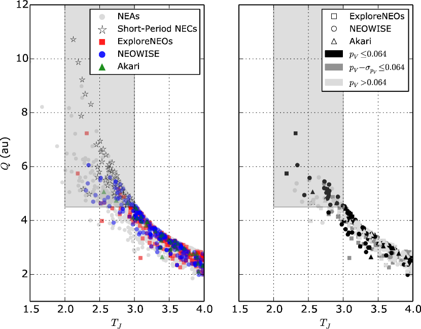
Figure 1: Left: $Q$ as a function of $T_{J}$ for near-Earth asteroids and short-period near-Earth comets. Gray dots represent known NEAs, star symbols are known short-period NECs; red squares are ExploreNEOs targets, blue circles are NEOWISE targets, green triangles are Akari targets. We select dormant comet candidates from the shaded area, which contains all known short-period near-Earth comets with $2.0\leq T_{J}\leq 3.0$ and 4.3% of all known NEAs. Right: Distribution of NEAs for which the albedo has been measured. Black symbols have albedos $p_{V}\leq 0.064$, dark gray symbols agree with the albedo limit within one standard deviation, and light-gray symbols have higher albedos. We find 51% of the NEAs with $Q\geq 4.5$ au and $2.0\leq T_{J}\leq 3.0$ to have comet-like albedos (see Section 4).

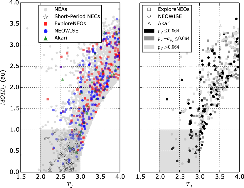
Figure 2: Left: $MOID_{J}$ as a function of $T_{J}$ for near-Earth asteroids and short-period near-Earth comets. Gray dots represent known NEAs, star symbols are known short-period NECs; red squares are ExploreNEOs targets, blue circles are NEOWISE targets, green triangles are Akari targets. We select dormant comet candidates from the shaded area, which contains 97% of all known short-period NECs and 3.6% of all known NEAs. Right: Distribution of NEAs for which the albedo has been measured. Black symbols have albedos $p_{V}\leq 0.064$, dark gray symbols agree with the albedo limit within one standard deviation, and light-gray symbols have higher albedos. In this case, we find 45% of the NEAs with $2.0\leq T_{J}\leq 3.0$ and $MOID_{J}\leq 1.0$ au to have comet-like albedos.

2.1 Tisserand Parameter

The “Tisserand parameter” is a dynamical quantity that is diagnostic of gravitational interaction of a body with a planet and is approximately conserved during encounters in the restricted three-body problem. The Tisserand parameter with respect to Jupiter is defined as

$$T_{J}=\frac{a_{J}}{a}+2\sqrt{\frac{a}{a_{J}}\left(1-e^{2}\right)}\cos{i},$$ (1)

where $a$, $e$, and $i$ are the semimajor axis, eccentricity, and inclination of the target body, respectively, and $a_{J}$ is the semimajor axis of Jupiter (Tisserand, 1896). $T_{J}$ is of special interest in orbital dynamics as it can be used as an approximate discriminator between asteroidal ($T_{J}>3.0$) and cometary ($T_{J}\leq 3.0$) orbits. The actual $T_{J}$-boundary between asteroids and comets is less strict, since $T_{J}$ is only conserved in the idealized case of the restricted three-body problem. Comets with $T_{J}>3.0$ exist and are called “Encke-type” comets. Only a few Encke-type comets are known and their origin is still subject to debate (Levison et al., 2005). Halley-type and long-period comets usually have $T_{J}<2$. In this work, we will neglect both long-period/Halley-type comets and Encke-type comets and only focus on short-period NECs. Levison & Duncan (1997) define short-period comets as comets with $2<T_{J}<3$, which allows the comets to experience low-velocity encounters with Jupiter. Hence, such comets are dynamically dominated by Jupiter, coining the term “Jupiter family comets”.

We use $T_{J}$ as determined by the JPL Small-Body Database Search Engine for both NEAs and NECs. For NEAs we use the same criterion that is used for the short-period NECs: $2.0\leq T_{J}\leq 3.0$. Previous works (Fernández et al., 2005; DeMeo et al., 2008; Kim et al., 2014) used the less strict criterion $T_{J}\leq 3.0$, potentially including a number of Halley-type comets.

2.2 Aphelion Distance

Comets have been scattered into the inner Solar System as a result of close encounters with Jupiter (Levison & Duncan, 1997). In order to be able to have somewhat close encounters with Jupiter, any object is required to have a sufficiently large aphelion distance $Q$ to feel the gravitational pull of the giant planet. The distribution of comets in $T_{J}$-$Q$ space (Figure 1, left plot) suggests $Q\geq 4.5$ au, which we adopt as our criterion for a cometary orbit in $Q$. Our criteria in $T_{J}$ and $Q$ apply to all short-period NECs but only 4.3% of the NEAs. Similar criteria have been adopted by Kim et al. (2014).

2.3 Minimum Orbit Intersection Distance

The “minimum orbit intersection distance” with Jupiter, $MOID_{J}$, describes the shortest distance between the orbit of a body and that of the giant planet. Hence, it defines the distance of the closest encounter both bodies can possibly have. Sosa et al. (2012) show that comets in near-Earth space are more likely to have a low $MOID_{J}$ than asteroids (their Figure 1). $MOID_{J}$ of both NEAs and short-period NECs has been calculated using the code provided by Wiźniowski & Rickman (2013). Since $MOID_{J}$ is not a dynamical invariant, we can only look at a snapshot image of the dynamical characteristics of the asteroid and comet populations. The deductions we can make are still justified, since we use a statistical approach to identify dormant comets in the NEA population. From Figure 2 (left plot) it is obvious that most short-period NECs have $MOID_{J}\leq 1.0$ au, which we adopt as our criterion. 97% of the short-period NEC population, and only 3.6% of the known NEA population meet this criterion.

2.4 Albedo

Cometary nuclei have low geometric albedos, $p_{V}$. Lamy et al. (2004) compiled a list of measured cometary nuclei albedos, most of which have $p_{V}\leq 0.05$. In their search for extinct cometary objects, Fernández et al. (2005) use an albedo upper limit of $p_{R}\leq 0.075$, which is based on albedo determinations of comets in the $R$ band, compiled in Lamy et al. (2004), and an assumed albedo uncertainty of 30%. We take an approach that is similar to that of Fernández et al. (2005), and define an upper limit for cometary $V$-band albedos based on previously measured albedos of short-period comets. In Table 1 we show the measured $V$-band albedos for the small number of short-period comet nuclei for which this information has been determined. From the measured albedos we determine the mean albedo $\langle p_{V}\rangle$ to be $0.047\pm 0.017$, where the uncertainty is the quadratic sum of the standard deviation and the root mean square of the uncertainties of the individual objects listed in Table 1. Our approach to estimating this uncertainty takes into account both internal and external uncertainties, i.e., it includes the uncertainties of the individual albedo measurements as well as the scatter of the ensemble of albedos. It is our intention to determine an upper-limit albedo for short-period comets, so we define our albedo limit as the mean value and add the uncertainty of 0.017, yielding $p_{V}\leq 0.064$. This limit includes all the comet albedos listed in Table 1 and is comparable to, but slightly lower than, the Fernández value (we obtain $p_{R}=0.071$ instead of 0.075), assuming a typical normalized spectral reflectivity gradient for comets of $10\%/1000$Å (Lamy et al., 2004).

Table 1: $V$-band Albedos of Short-Period Comets.

Name	$p_{V}$	Reference
2P/Encke	0.046$\pm$0.023	Fernández et al. (2000)
9P/Tempel 1	0.056$\pm$0.007	Li et al. (2007)
10P/Tempel 2	0.03$\pm$0.01	Campins et al. (1995)
22P/Kopff	0.042$\pm$0.006	Lamy et al. (2002)
28P/Neujmin 1	0.06$\pm$0.01	Campins et al. (1995)
49P/Arend-Rigaux	0.04$\pm$0.01	Campins et al. (1995)
67P/Churyumov-Gerasimenko	0.059$\pm$0.02	Sierks et al. (2015)
81P/Wild 2	0.059$\pm$0.004	Li et al. (2009)
103P/Hartley 2	0.028$\pm$0.009	Lisse et al. (2009)

Note. — This compilation of $V$ band albedos yields an average value of $\langle p_{V}\rangle=0.047\pm 0.017$. The albedo uncertainty of 49P has been recalculated based on the diameter uncertainty given by Campins et al. (1995).

3 NEA Sample

We base our search for dormant comets on NEA albedo measurements from our Warm Spitzer “ExploreNEOs” program (Trilling et al., 2010), as well as from the NEOWISE (Mainzer et al., 2011) and Akari (Usui et al., 2011) programs.

As part of ExploreNEOs we performed 589 observations (e.g., Trilling et al., 2010; Mueller et al., 2011; Trilling et al., under review) of 562 different optically discovered NEAs using the Infrared Array Camera (Fazio et al., 2004) onboard the Spitzer Space Telescope (Werner et al., 2004) at 3.6 and 4.5 $\mu$m. For each asteroid we derive diameter and albedo using the Near-Earth Asteroid Thermal Model (NEATM, Harris, 1998). Three of our targets were not considered in the papers quoted above due to detector saturation. 3552 Don Quixote was saturated in both IRAC channels and displayed cometary activity during the time of our observations (Mommert et al., 2014). Two more targets, 4015 Wilson-Harrington and 52762 (1998 MT24) were saturated in the 4.5 $\mu$m band, only. In order to derive flux densities from saturated images, we fit a calibrated point-spread function (PSF) model to the extended wings of the measured PSF, ignoring the saturated parts of the image. This method has been well tested on a number of saturated observations of calibration stars (see, e.g., Mommert et al., 2014, and references therein). We add an additional 5% uncertainty in quadrature to those flux densities to account for the increased calibration uncertainty. Three other targets, 2004 QF1, 152952 (2000 GC2), and 162825 (2001 BO61) were too faint to be detected in the 3.6 $\mu$m band, and results are based on the 4.5 $\mu$m flux density measurement only.

In order to determine accurate albedos, precise measurements of the absolute magnitude $H$ (the magnitude of an object at 1 au distance from the observer and the Sun, and at zero phase angle) and of the photometric slope parameter $G$ are crucial. In the ExploreNEOs program, we obtain $H$ magnitudes from the JPL Horizons service (Giorgini et al., 1996). The provided $H$ magnitudes are notoriously unreliable (Jurić et al., 2002; Pravec et al., 2012) and do not come with uncertainty estimates. Therefore, we replace these $H$ magnitudes by values taken from peer-reviewed publications (Hagen et al., under review; Pravec et al., 2012) (87 updates by Hagen, 29 by Pravec), where available. Where no measured values are available, we have to rely on the JPL Horizons $H$ magnitudes.

We increase our sample size by adding albedo measurements from 471 observations of 409 different NEAs observed by the NEOWISE program (Mainzer et al., 2011), excluding those NEAs for which albedo has not been measured. The Wide-field Infrared Survey Explorer (WISE, Wright et al., 2010) carried out an all-sky survey in its 3.4, 4.6, 12, and 22 $\mu$m bands. The design of the WISE survey enables it to discover new NEAs and comets in the thermal infrared, which minimizes the impact of albedo dependent discovery bias. NEOWISE also measures the diameters and albedos of all detected objects using the NEATM, using an approach that is similar to ExploreNEOs (Trilling et al., 2010; Mueller et al., 2011; Mainzer et al., 2011). We use updated albedos of 26 NEOWISE sample targets from Pravec et al. (2012) that are based on new measurements of $H$.

Furthermore, we add 59 NEAs from the “Asteroid catalog using Akari” (Usui et al., 2011), which is based on an all-sky survey in two mid-infrared bands (S9W: 6.7-11.6 $\mu$m, L18W: 13.9-25.6 $\mu$m), from which diameters and albedos have been derived using the Standard Thermal Model (STM, Morrison & Lebofsky, 1979; Lebofsky et al., 1986).

The combined samples comprise 1132 albedo measurements of 869 different NEAs, representing ${\sim}7\%$ of the known NEA population as of April 2015. Usui et al. (2014) performed a comparison of diameters and albedos measured for main belt asteroids between IRAS, Akari, and NEOWISE. They find an average agreement within 10% for diameter and 22% for albedo measurements between the three surveys. A similar comparison of 110 NEAs observed by ExploreNEOs and NEOWISE shows an equally good agreement within 6% in diameter and 22% in albedo on average (Trilling et al., under review).

4 Results

Of the 869 different NEAs with measured albedo, 65 have $2.0<T_{J}<3.0$ (see discussion in Section 3). Of those, 43 meet our additional $Q$ criterion and 31 meet our $MOID_{J}$ criterion, fulfilling our dynamical criteria for being cometary. Their albedos were analyzed in a second step: for both populations we performed a weighted count of the number of objects with $p_{V}\leq 0.064$. Table 4 lists all observations of asteroids for which at least one albedo measurement (23 NEAs) with $p_{V}\leq 0.064$ exists. NEAs 385402 (2002 WZ2) and (2000 HD74) each have one measurement with $p_{V}\leq 0.064$ and one with $p_{V}>0.064$. This discrepancy is most likely caused by lightcurve effects and the fact that both measurements use the same $H$ magnitude, which is not corrected for lightcurve effects. We reduce the weight of both objects in the following analysis to 0.5, whereas all other objects for which only $p_{V}\leq 0.064$ measurements exist have a weight of 1. For the $Q$-selected objects we hence find a statistical weight of 22 for a total of 43 NEAs with measured albedos; 22/43 = 51% (of the sample size) of the NEAs with $Q\geq 4.5$ au also have $p_{V}\leq 0.064$. For the $MOID_{J}$-selected sample, the weighted count is 14/31 (45% of the sample size). Note that all $MOID_{J}$-selected asteroids with $p_{V}\leq 0.064$ are also in the sample of $Q$-selected asteroids with $p_{V}\leq 0.064$.

The overlap of those NEAs in the $Q$-selected (43 NEAs) and $MOID_{J}$-selected (31 NEAs) samples with any albedo value is 24 objects, which is 56% of the $Q$-selected and 77% of the $MOID_{J}$-selected sample. Figures 1 and 2 (left plots) support the impression that in the $Q$-selected NEA sample, the ratio of cometary over asteroidal objects might be lower than for the $MOID_{J}$-selected sample. Nevertheless, the fact that in both dynamically selected samples about 50% of the objects have $p_{V}\leq 0.064$ suggests a similar degree of mixing between potential dormant comets ($p_{V}\leq 0.064$) and ordinary asteroids (any $p_{V}$) for both dynamical criteria. We consider the $Q$-selected sample of NEAs with $p_{V}\leq 0.064$, which includes the $MOID_{J}$-selected sample in its entirety, to be our sample of dormant short-period comet candidates in the NEA population.

Table 2: Dormant Short-Period Near-Earth Comet Candidates.

Object Name	$d$	$p_{V}$	$T_{J}$	$MOID_{J}$	$Q$	$H$	Source
	(km)			(au)	(au)	(mag)
3552 Don Quixote (1983 SA)	$18.4^{+0.3}_{-0.4}$	$0.03^{+0.02}_{-0.01}$	2.314	0.551	7.234	13.0	EN
5370 Taranis (1986 RA)	$5.31^{+0.08}_{-0.08}$	$0.051^{+0.009}_{-0.009}$	2.731	0.294	5.446	15.2	NW
5370 Taranis (1986 RA)	$6.3^{+0.5}_{-0.5}$	$0.037^{+0.009}_{-0.009}$	2.731	0.294	5.446	15.2	NW
20086 (1994 LW)	$4.8^{+1.3}_{-1.1}$	$0.013^{+0.014}_{-0.007}$	2.770	(1.197)	5.168	16.9	EN
248590 (2006 CS)	$4.7^{+0.8}_{-0.8}$	$0.018^{+0.007}_{-0.007}$	2.441	0.267	4.945	16.6	NW
385402 (2002 WZ2)	$2.3^{+0.7}_{-0.6}$	$0.06^{+0.07}_{-0.03}$	2.515	(2.482)	4.638	17.0	EN
385402 (2002 WZ2)	$1.6^{+0.1}_{-0.1}$	($0.11^{+0.03}_{-0.03}$)	2.515	(2.482)	4.638	17.0	NW
(2000 HD74)	$1.9^{+0.5}_{-0.5}$	$0.03^{+0.03}_{-0.02}$	2.567	(1.432)	4.662	18.0	EN
(2000 HD74)	$0.83^{+0.01}_{-0.01}$	($0.16^{+0.03}_{-0.03}$)	2.567	(1.432)	4.662	18.0	NW
(2001 HA4)	$1.85^{+0.04}_{-0.04}$	$0.05^{+0.01}_{-0.01}$	2.772	(1.515)	4.814	17.6	NW
(2004 EB)	$2.5^{+0.2}_{-0.2}$	$0.04^{+0.01}_{-0.01}$	2.755	(1.138)	5.176	17.2	NW
(2004 YR32)	$2.3^{+0.3}_{-0.3}$	$0.031^{+0.007}_{-0.007}$	2.725	(1.620)	5.203	17.6	NW
(2004 YZ23)	$9.4^{+4.3}_{-3.1}$	$0.02^{+0.02}_{-0.01}$	2.186	(1.722)	5.742	15.2	EN
(2009 KC3)	$2.2^{+0.5}_{-0.5}$	$0.023^{+0.018}_{-0.018}$	2.728	0.248	5.451	18.0	NW
(2009 WF104)	$2.23^{+0.03}_{-0.03}$	$0.047^{+0.009}_{-0.009}$	2.800	(1.342)	5.096	17.2	NW
(2009 WO6)	$2.49^{+0.01}_{-0.01}$	$0.034^{+0.008}_{-0.008}$	2.785	0.810	4.881	17.3	NW
(2009 XE11)	$2.72^{+0.02}_{-0.02}$	$0.038^{+0.006}_{-0.006}$	2.796	0.952	5.336	17.0	NW
(2010 AG79)	$0.89^{+0.01}_{-0.01}$	$0.018^{+0.003}_{-0.003}$	2.814	0.858	4.587	20.2	NW
(2010 DH77)	$0.63^{+0.02}_{-0.02}$	$0.009^{+0.002}_{-0.002}$	2.516	(1.401)	5.581	21.8	NW
(2010 DH77)	$0.52^{+0.02}_{-0.02}$	$0.012^{+0.003}_{-0.003}$	2.516	(1.401)	5.581	21.8	NW
(2010 FJ81)	$0.42^{+0.01}_{-0.01}$	$0.049^{+0.009}_{-0.009}$	2.341	0.577	6.056	20.8	NW
(2010 FJ81)	$0.5^{+0.1}_{-0.1}$	$0.03^{+0.02}_{-0.02}$	2.341	0.577	6.056	20.8	NW
(2010 FZ80)	$0.87^{+0.01}_{-0.01}$	$0.018^{+0.004}_{-0.004}$	2.755	0.509	4.796	20.3	NW
(2010 JL33)	$1.78^{+0.03}_{-0.03}$	$0.047^{+0.009}_{-0.009}$	2.910	0.898	4.637	17.7	NW
(2010 LR68)	$2.3^{+0.2}_{-0.2}$	$0.017^{+0.004}_{-0.004}$	2.923	0.606	4.882	18.3	NW
(2010 LV108)	$0.23^{+0.01}_{-0.01}$	$0.029^{+0.005}_{-0.005}$	2.994	0.517	4.553	22.6	NW
(2010 GX62)	$0.62^{+0.01}_{-0.01}$	$0.041^{+0.007}_{-0.007}$	2.757	0.885	5.031	20.2	NW
(2010 GX62)	$1.12^{+0.01}_{-0.01}$	$0.012^{+0.002}_{-0.002}$	2.757	0.885	5.031	20.2	NW
(2011 BX18)	$3.0^{+0.7}_{-0.7}$	$0.012^{+0.011}_{-0.006}$	2.793	0.985	4.976	18.0	EN

Note. — NEAs with orbits and albedos that resemble those of short-period NECs ($2\leq T_{J}\leq 3.0$ and ($Q\geq 4.5$ au or $MOID_{J}\leq 1.0$ au) and $p_{V}\leq 0.064$). For each object we list its diameter $d$, geometric albedo $p_{V}$, $T_{J}$, $MOID_{J}$, $Q$, absolute magnitude $H$, and source reference of the albedo measurement. Values in parentheses signal that the respective criterion has not been met (see Section 2).

References. — EN: ExploreNEOs (this work; Trilling et al., 2010, under review; Mommert et al., 2014); NW: NEOWISE (Mainzer et al., 2011; Pravec et al., 2012); AK: Akari (Usui et al., 2011)

Figure 3 compares the albedo distributions of different samples of NEAs with $2.0\leq T_{J}\leq 3.0$ as a function of $T_{J}$. In both the $Q$ and $MOID_{J}$-selected samples there is no obvious trend of lower albedo with decreasing $T_{J}$, since high albedos can be found irrespective of $T_{J}$. Interestingly, we do not find any NEAs with $p_{V}\leq 0.064$ for $2.0\leq T_{J}\leq 2.8$ that is not in either the $Q$ or the $MOID_{J}$-selected samples (Figure 3). We discuss the implications of the different albedo distributions in Section 5.2.

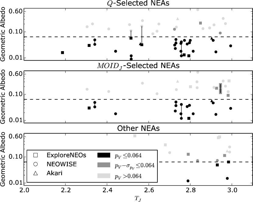
Figure 3: Albedos of NEAs with $2.0\leq T_{J}\leq 3.0$ as a function of $T_{J}$ for samples selected based on $Q$ and $MOID_{J}$, as well as the exclusive sample (“Other NEAs”). Black symbols refer to NEAs with $p_{V}\leq 0.064$, dark gray symbols to objects with $p_{V}-\sigma\leq 0.064$ (where $\sigma$ is the lower $1\sigma$ albedo uncertainty), and light gray symbols to objects with $p_{V}>0.064$. The dashed line indicates $p_{V}=0.064$, our albedo upper limit for comet-like albedos. For objects with more than one albedo measurement, the individual datapoints are connected with lines. We do not find any low-albedo NEAs with $T_{J}\leq 2.8$ that are neither in the $Q$ nor the $MOID_{J}$-selected samples. For the sake of readability, error bars are not shown; typical albedo relative uncertainties are of the order of 50%.

5 Discussion

5.1 Assessment of the Dormant Comet Fraction in the NEA Population

Based on our identification of dormant short-period near-Earth comet candidates in Section 4, we investigate the fraction of dormant short-period NECs in the NEA population. The discovery of dormant comets through optical surveys, which discover the majority of NEAs, is hampered for two reasons: highly eccentric, comet-like orbits mean that dormant comets spend most of their time far from the Earth, and their low albedos limit their optical brightness. Both factors have to be taken into account to obtain a reliable estimate of the dormant comet content.

In order to minimize the impact of discovery bias, we base this analysis of the dormant comet fraction solely on the NEOWISE sample. The nature of the NEOWISE survey as an all-sky survey in the thermal infrared provides a uniform sample of the NEA population that is much less affected by albedo bias than optical surveys (e.g., Mainzer et al., 2011). Using technical details on the NEOWISE survey from Wright et al. (2010) and Mainzer et al. (2011), we produce a NEOWISE survey simulator in order to de-bias the NEA population as observed by WISE. For a detailed description of the survey simulator we refer to Appendix A.

Using our NEOWISE simulator, we derive the dormant short-period NEC fraction in a magnitude-limited and a size-limited sample of the NEA population. Table 4 lists only a few dormant comet candidates with $H>21$ that were observed by NEOWISE. Hence, we decide to restrict our magnitude-limited sample to $H\leq 21$, which includes 17 dormant comet candidates (see Table 4) with diameters larger than ${\sim}400$m, assuming an albedo of 0.047. In order to properly account for albedo and absolute magnitude uncertainties of each object, we vary both parameters according to Gaussian statistics. We adopt the measured albedo uncertainty (see Table 4) as the 1$\sigma$ uncertainty, and in the case of the absolute magnitude, we adopt a 1$\sigma$ uncertainty of 0.2 mag, which is based on results by Jurić et al. (2002). From 100 trials with varied physical properties, we find that 0.3–3.3% (1$\sigma$ confidence interval) of the NEA population with $H\leq 21$ can be considered dormant short-period NECs.

For our size-limited estimate of the dormant short-period NEC fraction we consider NEAs with diameters $d\geq 1$ km, a size range that is well-sampled by NEOWISE and nearly entirely discovered (Mainzer et al., 2011). Using the same method as above, we vary the diameter and albedo within the NEOWISE-derived uncertainties and run the simulation 100 times. We find that $(9_{-5}^{+2})$% (1$\sigma$) of the NEA population with $d\geq 1$ km are dormant short-period NECs. In combination with the estimate of the number of NEAs with $d\geq 1$ km by Mainzer et al. (2011), we conclude that ${\sim}$100 NEAs with diameters of 1 km or more are dormant comets.

We note that these estimates differ significantly. We attribute this discrepancy to two different effects. Due to the albedo-dependence of the absolute magnitude and the wide range of albedos in the NEA population, high-albedo NEAs are over-represented in the magnitude-selected sample. Hence, one would expect a smaller fraction of dormant comets in the magnitude-selected sample, compared to the size-selected one. Furthermore, one has to account for the different slopes of the size-frequency distributions of NEAs and comets (compare to, e.g., Meech et al., 2004; Mainzer et al., 2011; Trilling et al., under review), the latter of which is more shallow due to the disintegration of small cometary objects with low perihelion distances. We find that the uncertainties we obtain for both fractions are well within the confidence ranges we derive in Appendix A.2.

We compare our findings with earlier estimates of the dormant comet fraction in the NEA population. Bottke et al. (2002) used dynamical simulations of a de-biased synthetic NEA population to estimate the fraction of cometary objects in the NEA population and found a fractional content of ($6\pm 4$)% in the magnitude-limited NEA population with $13<H<22$. Our magnitude-limited estimate, 0.3–3.3%, is lower than but partly overlaps with their estimate, covering nearly the same range in magnitude (we use $H\leq 21$). Fernández et al. (2005) based their assessment on albedo measurements of 10 dynamically selected NEAs. Their sample selection was solely based on observability, is therefore not de-biased, and has to be assumed to be magnitude-limited. From their target sample they selected objects on comet-like orbits with $T_{J}\leq 3.0$ and albedos $p_{R}\leq 0.075$. They find 4% of all NEAs to be of cometary origin. Our magnitude-limited result, 0.3–3.3%, is slightly lower than their result. DeMeo et al. (2008) based their analysis on 39 NEAs with $T_{J}\leq 3.0$. In order to identify cometary object candidates, they either require $p_{R}\leq 0.075$ or a C, D, T, or P taxonomic classification of the object. Furthermore, they base their result on the assumption that 30% of all NEAs with $d\geq 1$ km have $T_{J}\leq 3.0$ (Stuart, 2003). They find that ($8\pm 5$)% of all NEAs with $d\geq 1$ km are dormant comets. We find that $(9_{-5}^{+2})$% of NEAs with $d\geq 1$ km are dormant comets which is in good agreement with their result. Whitman et al. (2006) estimate a total of ${\sim}75$ dormant comets in the NEA population with $H<18$. Assuming an albedo of 0.047, this magnitude limit is equal to sizes of $d>1.5$ km. Our size-limited estimate infers a total of ${\sim}100$ dormant comets in the NEA population with $d\geq 1$ km, which is of the same order of magnitude.

5.2 Albedo Distribution of NEAs on Comet-Like Orbits

In Figure 3 we compare the albedo distributions of the $Q$ and $MOID_{J}$-selected samples as a function of $T_{J}$. Fernández et al. (2005) found that of the 9 NEAs they analyzed with $2.0\leq T_{J}\leq 3.0$ (6 of their own from which we exclude 2008 OG108 for being a comet, and 4 from the literature), 44% have nominal albedos $p_{R}\leq 0.075$ and 66% have albedos $p_{R}\leq 0.075$ within the uncertainties. We find that ${\sim}$50% of NEAs on comet-like orbits also have comet-like albedos, which is in good agreement with their result. Fernández et al. (2005) have 2 NEAs in their sample with $T_{J}\leq 2.6$, both of which have comet-like albedos, potentially suggesting that NEAs with $T_{J}\leq 2.6$ are more likely to have comet-like albedos. We find that the ratio of comet-like albedos to non-comet-like albedos is approximately constant for the intervals $2.0\leq T_{J}\leq 2.6$ and $2.6\leq T_{J}\leq 3.0$. Hence, the findings from this work and others (Fernández et al., 2005; Kim et al., 2014) suggest that the albedo distribution of NEAs on comet-like orbits is less strictly correlated to the dynamical distribution than previously expected. This heterogeneity implies that not all NEAs on comet-like orbits have a cometary origin. Potential asteroids that move on supposedly comet-like orbits have been identified by Fernández et al. (2014), who performed orbital integrations of a sample of NEAs on comet-like orbits. Most of these objects, which probably originate from the asteroid main belt, are likely to have higher than cometary albedos, accounting for the observed albedo diversity.

We also compare the albedo distributions of NEAs in the $Q$ and $MOID_{J}$-selected samples with those “other” NEAs that are in neither of the two samples. We find that none of the “other” NEAs with measured physical properties and $2.0\leq T_{J}\leq 2.8$ has a low albedo ($p_{V}\leq 0.064$). We estimate the probability of any interlopers, non-cometary NEAs with $2.0\leq T_{J}\leq 2.8$ and $p_{V}\leq 0.064$, to not meet either the $Q$ or the $MOID_{J}$ criterion. Based on the 23 dormant short-period NEC candidates with $2.0\leq T_{J}\leq 2.8$, the probability of a newly discovered NEA with the same properties not to be dormant short-period NEC candidate is ${\leq}1/(23+1)=4\%$. We conclude that any NEA with $2.0\leq T_{J}\leq 2.8$ and $p_{V}\leq 0.064$ has a ${\geq}$96% probability to be of cometary origin.

6 Conclusions

From our search for dormant short-period near-Earth comets in the NEA population we can draw the following conclusions:

• We identify 23 NEAs with orbits and albedos resembling those of short-period NECs that can be considered dormant short-period NECs.

• From a de-biasing of the NEOWISE survey, we find that 0.3–3.3% of the NEAs with $H\leq 21$ and $(9_{-5}^{+2})$% of those with $d\geq 1$ km can be considered dormant short-period NEC candidates. The magnitude-limited fraction is slightly lower than earlier estimates, whereas the size-limited fraction agrees with earlier estimates. We estimate that ${\sim}$100 NEAs with diameters of 1 km or more are dormant short-period NECs.

• We find that only ${\sim}$50% of our sample NEAs on short-period NEC-like orbits have comet-like albedos, suggesting mixing between cometary and asteroidal objects among our sample targets. However, we find that any NEA with $2.0\leq T_{J}\leq 2.8$ and $p_{V}\leq 0.064$ has a ${\geq}$96% probability to be of cometary origin.

Appendix A NEOWISE Survey Simulator

We simulate the detectability of NEAs through the WISE all-sky survey (Wright et al., 2010; Mainzer et al., 2011) in order to account for biases inherent to the survey. The results of the simulator are utilized to obtain a picture of the NEA population that is much more complete and less prone to discovery bias. We determine the detection efficiency for WISE as a function of orbital and physical properties of the NEA, based on a simulated input NEA population, a simplified model of the WISE observation strategy (Wright et al., 2010), and the WISE detection efficiency in its most sensitive bands, W3 and W4 (Mainzer et al., 2011). The de-biased NEA population is then derived by dividing the sample of NEAs that were actually observed by WISE in its cryogenic mission phase (Mainzer et al., 2011) by the derived detection efficiencies. We base this analysis solely on the cryogenic part of the WISE mission, which provides data from the most sensitive bands (W3 and W4).

A.1 Method

Each object of the input NEA population is characterized by a set of orbital parameters (semimajor axis, $a$, eccentricity, $e$, inclination, $i$, the longitude of the ascending node, $\Omega$, the argument of the perihelion, $\omega$, and the mean anomaly, $M$, at the epoch) and physical properties (absolute magnitude, $H$, albedo, $p_{V}$, diameter, $d$, and thermal model beaming parameter $\eta$). Our input NEA population consists of 100000 NEAs derived with the NEA model by Greenstreet et al. (2012), to each of which we randomly assign physical properties that are in accordance with the distributions in $H$, $p_{V}$, and $\eta$ found by Mainzer et al. (2011). The synthetic input NEA population is summed up in a matrix $S=(a\times e\times i\times d\times p_{V})$, according to their orbital and physical properties, i.e., each cell of the matrix holds the number of objects with a specific set of properties. Note that $d$ can be replaced by $H$ in matrix $S$ if the simulation is performed on a magnitude-limited instead of a size-limited sample; for the sake of simplicity we will only use $d$ in the following discussion. The set of actual NEOWISE detections throughout the cryogenic part of the WISE mission is read into a similar matrix, $R=(a\times e\times i\times d\times p_{V})$.

For each object in the input NEA population we determine its geocentric position for each day during the cryogenic part of the WISE mission (January 14 – August 5, 2010; 203 days) using the Python package PyEphem. WISE orbits in a low-Earth polar orbit and observes at 90° solar elongation (Wright et al., 2010). Hence, we determine times for which each object is in quadrature relative to the Earth. For each quadrature situation, we perform a more thorough check for WISE observability: for each 11 sec timestep (WISE observation cadence, Wright et al., 2010), we check if the object’s position coincides within 23.5′ (half-width of the WISE field of view) of the WISE pointing. The declination of WISE is assumed to follow a polar rotation with a period of 94.3 min, which has been derived from the orbital properties given by Wright et al. (2010). In accordance to the NEOWISE moving object pipeline specifications (Mainzer et al., 2011), we require each potentially detectable NEA to appear in at least 5 fields and to have a moving rate of 0.06–3.2° day^-1. This approach is simplified in such a way as it neglects the details of WISE pointing, e.g., with respect to the Moon.

In a second step, we estimate the thermal-infrared brightness of each potentially detectable object during each observability window. For each occassion in which an object is present in the WISE field of view, we derive its thermal emission at wavelengths 11.5608 $\mu$m (W3) and 22.0883 $\mu$m (W4) using the Near-Earth Asteroid Thermal Model (NEATM, Harris, 1998) and based on the physical and orbital properties of the object. The predicted thermal flux densities are compared to the measured sensitivity of the respective band (Equation 3 in Mainzer et al., 2011) and the detection probability in each band ($P_{W3}$, $P_{W4}$) is derived. The final detection probability of one object is defined as $max(P_{W3},P_{W4})$ over the cryogenic mission phase.

The detection probabilities of all objects from the input NEA population are summed up in a matrix similar to $S$, $P=(a\times e\times i\times d\times p_{V}$). The detection efficiency is derived as $E=P/S$ in an element-wise matrix division. Finally, the de-biased population, $D$, is derived by dividing the sample of NEAs observed during the cryogenic part of the WISE mission by the efficiency matrix, $D=R/E$ (element-wise).

A.2 Consistency Check

We test the consistency of the NEOWISE simulator with the real NEOWISE survey using two different tests. The first test compares the compatibility of simulator detections with the real survey using two exclusive samples: the sample of objects that was detected during the cryogenic part of the NEOWISE program (Mainzer et al., 2011) (“NEOWISE sample”, 471 detections) and those objects that were observed by the Spitzer Space Telescope in the framework of the ExploreNEOs program (Trilling et al., 2010), but not by the NEOWISE program (“ExploreNEOs-not-NEOWISE”, 460 detections). Ideally, the NEOWISE simulator detects all objects in the NEOWISE sample and none of those objects in the ExploreNEOs-not-NEOWISE sample. For this test, we use the actually measured physical properties (diameter, albedo, and $\eta$), as well as the real orbital elements for each object and run the simulation over the duration of the cryogenic WISE mission phase. We derive the completeness of each sample by summing up the detection probabilities of the individual objects and divide the sum by the total number of objects in each sample. We find that 88% of all NEOWISE-observed NEAs (12% false negatives) are detected by our simulator and only 7% of the ExploreNEOs-not-NEOWISE objects (7% false positives). Hence, the overall agreement in NEA detectability between the simulator and the real NEOWISE survey is good.

In a second test, we investigate the accuracy of our de-biasing technique by replicating the estimate of the number of 1 km-sized NEAs derived by Mainzer et al. (2011). We perform 100 simulator trials in which we vary the physical properties of the NEAs listed in Mainzer et al. (2011) within their uncertainties based on Gaussian statistics. In the case of objects that have more than one detection, we randomly reject duplicate detections such that every NEA appears only once in matrix $R$. We de-bias the 1 km NEA population by comparing the number of such objects that were detected by NEOWISE ($R_{d\geq 1\mathrm{~{}km}}$) with the number of objects in our synthetic input population ($S_{d\geq 1\mathrm{~{}km}}$). We find an average number of 1 km-sized NEAs of 1200${\pm}$150, which agrees within 1.5$\sigma$ with the number found by Mainzer et al. (2011), 981$\pm$19. Note that Mainzer et al. (2011) based their result on a more elaborate de-biasing technique, which takes into account more information about the known NEA population, whereas our approach can be considered a “blind” de-biasing that is only based on those NEAs detected by the NEOWISE survey. Hence, we consider the significance of the agreement between these results adequate.

References

- Binzel et al. (1992) Binzel, R. P., Xu, S., Bus, S. J., Bowell, E., 1992, Science , Vol. 257, 779
- Boehnhardt (2004) Boehnhardt, H. 2004, Comets II, M. C. Festou, H. U. Keller, and H. A. Weaver (eds.), University of Arizona Press, Tucson, 301
- Bottke et al. (2002) Bottke, W. F., Morbidelli, A., Jedicke, R. et al., 2002, Icarus, 156, 399
- Bowell et al. (1992) Bowell, E., West, R. M., Heyer, H.-H. et al., 1992, IAU Circ., 5585
- Campins et al. (1995) Campins, H., Osip, D. J., Rieke, G. H., Rieke, M. J., 1995, Planetary and Space Sciences, 43, 733
- Delsemme (1984) Delsemme, A. H., 1984, Origins of Life, 14, 51
- DeMeo et al. (2008) DeMeo, F., Binzel, R. P., 2008, Icarus, 194, 436
- Duncan et al. (2004) Duncan, M., Levison., H., Dones, L., 2004, Comets II, M. C. Festou, H. U. Keller, and H. A. Weaver (eds.), University of Arizona Press, Tucson, 193
- Fazio et al. (2004) Fazio, G. G., Hora, J. L, Allen, L. E. et al., 2004, ApJS, 154, 10
- Fernández et al. (1997) Fernández, Y. R., McFadden, L. A., Lisse, C. M. et al., 1997, Icarus, 128, 114
- Fernández et al. (2000) Fernández, Y. R., Lisse, C. M., Käufl, H. U. et al., 2000, Icarus, 147, 145
- Fernández et al. (2005) Fernández, Y. R., Jewitt, D. C., & Sheppard, S. S., 2005, AJ, 130, 308
- Fernández et al. (2014) Fernández, J. A., Sosa, A., Gallardo, T., and Gutiérrez, J. N., 2014, Icarus, 238, 1
- Giorgini et al. (1996) Giorgini, J. D., Yeomans, D. K., Chamberlin, A. B. et al. 1996, Bulletin of the American Astronomical Society, 28, 1158
- Greenstreet et al. (2012) Greenstreet, S., Ngo, H., Gladman, B, 2012, Icarus, 217, 355
- Hagen et al. (under review) Hagen, A. R., Trilling, D. E., Penprase, B. E. et al., AJ, under review
- Hahn & Rickman (1985) Hahn, G. and Rickman, H. 1985, Icarus, 61, 417
- Harris (1998) Harris, A. W., 1998, Icarus, 131, 291
- Hartogh et al. (2011) Hartogh, P., Lis, D. C., Bockelée-Morvan, D., de Val-Borro, M., Biver, N. et al. 2011, Nature, 478, 218
- Jurić et al. (2002) Jurić, M., Iveziź, Ž, Lupton, R. H., 2002, AJ, 124, 1776
- Kim et al. (2014) Kim, Y., Ishiguro, M., Usui, F., 2014, ApJ, 789, 151
- Lamy et al. (2002) Lamy, P. L., Toth, I., Jorda, L. et al., 2002, Icarus, 156, 442
- Lamy et al. (2004) Lamy, P. L., Toth, I., Fernandez, Y. R., Weaver, H. A., 2004, Comets II, M. C. Festou, H. U. Keller, and H. A. Weaver (eds.), University of Arizona Press, Tucson, 223
- Lebofsky et al. (1986) Lebofsky, L. A., Sykes, M. V., Tedesco, E. F. et al. 1986, Icarus, 86, 239
- Levison & Duncan (1997) Levison, H., Duncan, M., 1997, Icarus, 127, 13
- Levison et al. (2005) Levison, H., Terrell, D., Wiegert, P. A., Dones, L., Duncan, M. J., 2005, Icarus, 182, 161
- Levison et al. (2006) Levison, H., Duncan, M. J., Dones, L., Gladman, B. J. 2006, Icarus, 184, 619
- Li et al. (2007) Li, J.-Y., A’Hearn, M. F., Belton, M. J. S. et al., 2007, Icarus, 187, 41
- Li et al. (2009) Li, J.-Y., A’Hearn, M. F., Farnham, T. L., McFadden, L. A., 2009, Icarus, 204, 209
- Lisse et al. (2009) Lisse, C. M., Fernández, Y. R., Reach, W. T., Bauer, J. M., A’Hearn, M. F. et al. 2009, PASS, 121, 968
- Lowry et al. (2008) Lowry, S., Fitzsimmons, A., Lamy, P., Weissman, P., 2008, The Solar System Beyond Neptune, M. A. Barucci, H. Boehnhardt, D. P. Cruikshank, and A. Morbidelli (eds.), University of Arizona Press, Tucson, p.397
- Mainzer et al. (2011) Mainzer, A., Grav, T., Bauer, J. et al., 2011, ApJ, 743, 156
- Meech et al. (2004) Meech, K. J., Hainaut, O. R., Marsden, B. G. 2004, Icarus, 170, 463
- Mommert et al. (2014) Mommert, M., Hora, J. L., Harris, A. W. et al. 2014, ApJ, 781, 25
- Morbidelli & Gladman (1998) Morbidelli, A. and Gladman, B., 1998, Meteoritics & Planetary Science, 33, 999
- Morrison & Lebofsky (1979) Morrison, D. and Lebofsky, L. A. 1979, in Asteroids, ed: T. Gehrels (Tucson: Univ. Arizona Press), 184
- Mottl et al. (2007) Mottl, M. J., Glazer, B. T., Kaiser, R. I., Meech, K, J 2007, Chemie der Erde - Geochemistry, 67, 253
- Mueller et al. (2011) Mueller, M., Delbo’, M., Hora, J. L. et al., 2011, AJ, 141, 109
- Öpik (1963) Öpik, E. J., 1963, Adv. Astron. Astrophys., 2, 219
- Oró (1961) Oró, J., 1961, Nature, 190, 389
- Pravec et al. (2012) Pravec, P., Harris, A. W., Kušnirák, P., Galád, A., Hornoch, K., 2012, Icarus, 221, 365
- Sosa et al. (2012) Sosa, A., Fernández, J. A., Pais, P., 2012, A&A, 548, A64
- Sierks et al. (2015) Sierks, H., Barbieri, C., Lamy, P. L., Rodrigo, R., Koschny, D. et al. 2015, Science, 347, 1044
- Stuart (2003) Stuart, J. S., 2003, Doctoral thesis, Massachusetts Institute of Technology, Cambridge, MA.
- Tisserand (1896) Tisserand, F., 1896. Traité de Mécanique Céleste, Théories des satellites de Jupiter et de Saturne, vol. 4. Perturbations des petites planétes, Gauthier-Villars, Paris, p. 205.
- Trilling et al. (2010) Trilling, D. E., Mueller, M., Hora, J. L. et al., 2010, AJ, 140, 770
- Trilling et al. (under review) Trilling, D. E., Mommert, M., Mueller, M. et al., AJ, under review
- Usui et al. (2011) Usui, F., Kuroda, D., Müller, T. G. et al., 2011, PASJ, 63, 1117
- Vokrouhlický & Farinella (2000) Vokrouhlický, D., Farinella, P., 2000, Nature, 407, 606
- Usui et al. (2014) Usui, F., Hasegawa, S., Ishiguro, M., Müller, T. G., Ootsubo, T. 2014, PASJ, 66, 5611
- Wang & Brasser (2014) Wang, J.-H., Brasser, R. 2014, A&A, 563, 122
- Weissman (1996) Weissman, P. R., 1996. In Rettig, T. and Hahn, J. M., eds., Completing the Inventory of the Solar System, Astronomical Society of the Pacific Conference Series, volume 107, 265–288
- Werner et al. (2004) Werner, M. W., Roellig, T. L., Low, F. J., Rieke, G. H., Rieke, M. et al. 2004, ApJS, 154, 1
- Wetherill (1979) Wetherill, G. W., 1979, Icarus, 37, 96
- Wetherill (1988) Wetherill, G. W., 1988, Icarus, 76, 1
- Wetherill (1991) Wetherill, G. W., 1991, in: Comets in the post-Halley era., ed. R. L. Newburn, M. Neugebauer, J. Rahe (Dordrecht: Kluwer Academic Publishers), Vol. 1, 537
- Whitman et al. (2006) Whitman, K., Morbidelli, A., Jedicke, R., 2006, Icarus 183, 101
- Wisdom (1983) Wisdom, J., 1983, Icarus, 56, 51
- Wiźniowski & Rickman (2013) Wiźniowski, T., Rickman, H., 2013, Acta Astronomica, 63, 293
- Wright et al. (2010) Wright, E. L., Eisenhardt, P. R. M., Mainzer, A. K. et al., 2010, AJ, 140, 1868