Semiclassical solution to the BFKL equation with massive gluons

Abstract:

In this paper we proceed to study the high energy behavior of scattering amplitudes in a simple field model, with the Higgs mechanism for the gauge boson mass. The spectrum of the $j$-plane singularities of the $t$-channel partial waves, and corresponding eigenfunctions of the BFKL equation in leading log($1/x$) approximation (LLA), were previously calculated numerically. Here a semiclassical approach is developed to investigate the influence of the impact parameter exponential decrease, existing in this model, on the high energy asymptotic behaviour of the scattering amplitude. This approach is much simpler than the numerical calculations, and reproduces their results. The analytical (semi-analytical) solutions which have been found in the approximation, can be used to incorporate correctly the large impact parameter behavior in the framework of CGC/saturation approach. This behaviour is interesting as provides the high energy amplitude for the electroweak theory, which can be measured experimentally.

1 Introduction

In our paper [1] we solved the BFKL equation with a massive gluon in the framework of the Higgs model numerically. Such an equation arises in the electroweak theory with zero Weinberg angle ( see Ref.  [2]). However, for us, this gauge invariant theory provides an instructive example of a model in which the scattering amplitude has correct large impact parameter behavior ( scattering amplitude $\propto\exp\left(-m\,b\right)$ at large $b$), but we still have the unitarity problem as the scattering amplitude increases as $s^{\Delta}$ at high energies. Therefore, this model is a perfect training ground to study how the correct $b$ behavior, can influence the resolution of the unitarity problem in the framework of the CGC/saturation approach  [3, 4, 5, 6]. This approach leads to a partial amplitude smaller than unity, as required by unitarity constraints. However, it generates a radius of interaction that increases as power of energy  [7, 8, 9, 10], leading to the violation of the Froissart bound [11].

Another facet of this model, is that it is a possible candidate for an effective theory equivalent to perturbative QCD, in the region of distances ($r$) shorter than $1/m$, where $m$ denotes the gluon mass. Indeed, for $r\,\ll\,1/m$, the fact that gluon has a mass, is not essential while at $r\sim 1/m$ similar correlation functions arise from fixing or eliminating Gribov’s copies  [12] (see Refs.  [13, 14, 15]). We wish to stress that a gauge theory with the Higgs mechanism, leads to a good description of the gluon propagator, calculated in lattice approach [16] with $m=0.54\,GeV$. Therefore, a plausible scenario is that the Higgs gauge theory describes QCD in the kinematic region $r\,\leq 1/m$, while for $r\sim 1/\Lambda_{\mbox{\tiny QCD}}\,>\,1/m$ the non-perturbative QCD approach takes over, and leads to the confinement of quarks and gluons, which is missing in the theory with a massive gluon.

We found [1] that the spectrum of the massive BFKL equation in $\omega$-space for $t=0$, coincides with that of massless one  [17, 18]. The simple parametrization of the eigenfunctions have also been obtained in Ref. [1]. In this paper we propose using the solution to the BFKL equation with massive gluons which has an advantage of being simple and semi-analytic. Having this solution in hand, we are able to progress to more difficult problems, e.g. a generalization of the main equations of the CGC/saturation approach [19, 20, 6].

The equation for the scattering amplitude in leading $\ln(1/x)$ approximation of perturbative theory, has been on the market for some time  [17], and is schematically shown in the Fig. 1. Its kernel is of the form  [17, 1]

Figure 1: The massive BFKL equation (Fig. 1-a) and its kernel (Fig. 1-b)

$$K\left(q_{1},q_{2}|q^{\prime}_{1},q^{\prime}_{2}\right)\,\, = \frac{\alpha_{S}N_{c}}{2\pi^{2}}\Big{\{}\frac{1}{k^{2}+m^{2}}\Big{(}\frac{q^{2}_{1}+m^{2}}{q^{\prime 2}_{1}+m^{2}}\,+\,\frac{q^{2}_{2}+m^{2}}{q^{\prime 2}_{2}+m^{2}}\Big{)}\,\,-\,\,\frac{q^{2}+\frac{N^{2}_{c}+1}{N^{2}_{c}}m^{2}}{(q^{\prime 2}_{1}+m^{2})(q^{\prime 2}_{2}+m^{2})}\Big{\}}.$$ (1.1)

For $q=0$, the kernel (1.1) simplifies considerably, and yields a homogeneous BFKL equation for the Yang-Mills theory with the Higgs mechanism,

$$\omega f\left(p\right)\,\,=\,\,2\omega\left(p\right)f\left(p\right)\,+\,\frac{\alpha_{S}N_{c}}{2\pi^{2}}\int d^{2}p^{\prime}\Big{(}\frac{2f\left(p^{\prime}\right)}{\left(\vec{p}-\vec{p}^{\,\,{}^{\prime}}\right)^{2}+m^{2}}\,\,-\,\,\frac{\frac{N^{2}_{c}+1}{N^{2}_{c}}m^{2}\,f\left(p^{\prime}\right)}{(p^{2}+m^{2})(p^{\prime 2}+m^{2}}\Big{)},$$ (1.2)

where $q_{1}=q_{2}=p$, $q^{\prime}_{1}=q^{\prime}_{2}=p^{\prime}$ and $\omega(p)$ is the gluon Regge trajectory given by

$$\omega\left(p\right)\,\, = \,\,-\frac{\alpha_{S}N_{c}}{4\pi^{2}}\int\frac{d^{2}k\left(p^{2}+m^{2}\right)}{\left(k^{2}+m^{2}\right)\left(\left(\vec{p}-\vec{k}\right)^{2}+m^{2}\right)}\,=\,-\,\frac{\alpha_{S}N_{c}}{2\pi^{2}}\frac{p^{2}+m^{2}}{|p|\sqrt{p^{2}+4m^{2}}}\ln\frac{\sqrt{p^{2}+4m^{2}}+|p|}{\sqrt{p^{2}+4m^{2}}-|p|}.$$ (1.3)

Examining the rotationally symmetric solution, the kernel can be integrated over the azimuthal angle $\phi$. Introducing the new variables

$$\kappa\,=\,\frac{p^{2}}{m^{2}};\,\,\,\,\,\,\,\,\,\,\,\,\,\,\kappa^{\prime}\,=\,\frac{p^{\prime 2}}{m^{2}};\,\,\,\,\,\,\,\,\,\,\,\,\,E\,=\,-\frac{\omega}{\bar{\alpha}_{S}};\,\,\,\,\,\,\,\,\,\,\,\,\,\bar{\alpha}_{S}\,=\,\frac{\alpha_{S}N_{c}}{\pi},$$ (1.4)

and changing the notation of the wave function $f(p)$ to $\phi_{E}(\kappa)$, we obtain the one-dimensional BFKL equation

$$E\phi_{E}\left(\kappa\right)\,\,=\,\,T\left(\kappa\right)\,\phi_{E}\left(\kappa\right)\,\,-\,\,\int^{\infty}_{0}\,\frac{d\kappa^{\prime}\,\phi_{E}\left(\kappa^{\prime}\right)}{\sqrt{(\kappa-\kappa^{\prime})^{2}\,+\,2(\kappa+\kappa^{\prime})+1}}\,\,+\,\,\frac{N^{2}_{c}+1}{2N^{2}_{c}}\frac{1}{\kappa+1}\int^{\infty}_{0}\frac{\phi_{E}\left(\kappa^{\prime}\right)\,d\kappa^{\prime}}{\kappa^{\prime}+1},$$ (1.5)

where the kinetic energy is given by

$$T\left(\kappa\right)\,\,=\,\,\frac{\kappa+1}{\sqrt{\kappa}\sqrt{\kappa+4}}\ln\frac{\sqrt{\kappa+4}+\sqrt{\kappa}}{\sqrt{\kappa+4}-\sqrt{\kappa}}.$$ (1.6)

In this paper we will deal mostly with the wave function in $Y$ representation defined by a Fourier transform,

$$\Psi\left(Y,\kappa\right)\,=\,\int^{\epsilon+i\infty}_{\epsilon-i\infty}\frac{dE}{2\pi i}e^{-EY}\,\phi_{E}\left(\kappa\right).$$ (1.7)

For $\Psi\left(Y,\kappa\right)$, the Eq. (1.5) takes the form

$$\frac{\partial\Psi\left(Y,\kappa\right)}{\partial Y}=-T\left(\kappa\right)\Psi\left(Y,\kappa\right)+\int^{\infty}_{0}\,\frac{d\kappa^{\prime}\Psi\left(Y,\kappa^{\prime}\right)}{\sqrt{(\kappa-\kappa^{\prime})^{2}\,+\,2(\kappa+\kappa^{\prime})+1}}-\frac{N^{2}_{c}+1}{2N^{2}_{c}}\frac{1}{\kappa+1}\int^{\infty}_{0}\frac{\Psi\left(Y,\kappa\right)\,d\kappa^{\prime}}{\kappa^{\prime}+1}$$ (1.8)

For completeness of presentation, we recall that the massless BFKL equations have the following form

$$E\,\phi^{\mbox{\tiny BFKL}}_{E}\left(\kappa\right)\,\, \underset{\epsilon\,\to\,0}{=} \,\,\ln\left(\frac{\kappa}{\epsilon}\right)\,\phi^{\mbox{\tiny BFKL}}_{E}\,\,-\,\,\int^{\infty}_{0}\,\frac{d\kappa^{\prime}\,\phi^{\mbox{\tiny BFKL}}_{E}\left(\kappa^{\prime}\right)}{|\kappa\,-\,\kappa^{\prime}|\,+\,\sqrt{\kappa\,\epsilon}}=-\,\,\int^{\infty}_{0}\,\frac{d\kappa^{\prime}\,\left(\phi^{\mbox{\tiny BFKL}}_{E}\left(\kappa^{\prime}\right)-\phi^{\mbox{\tiny BFKL}}_{E}\left(\kappa^{\prime}\right)\right)}{|\kappa\,-\,\kappa^{\prime}|},$$

$$\frac{\partial\Psi^{\mbox{\tiny BFKL}}\left(Y,\kappa\right)}{\partial Y}\,\, \underset{\epsilon\,\to\,0}{=} \,\,-\ln\left(\frac{\kappa}{\epsilon}\right)\,\Psi^{\mbox{\tiny BFKL}}\left(Y,\kappa\right)\,\,+\,\,\int^{\infty}_{0}\,\frac{d\kappa^{\prime}\,\Psi^{\mbox{\tiny BFKL}}\left(Y,\kappa^{\prime}\right)}{|\kappa-\kappa^{\prime}|\,+\,\sqrt{\kappa\,\epsilon}}$$

The way of regularization at $\epsilon\to 0$ stems directly from Eq. (1.2) considering small masses $\epsilon\,m^{2}$ instead of $m^{2}$. Eq. (1) can then , be re-written with a different way of regularization, for example

$$E\,\phi^{\mbox{\tiny BFKL}}_{E}\left(\kappa\right)\,\,\underset{\epsilon\,\to\,0}{=}\,\,-\ln\left(\frac{\epsilon^{2}}{2}\right)\,\phi^{\mbox{\tiny BFKL}}_{E}\,\,-\,\,\int^{\infty}_{0}\,d\kappa^{\prime}\,\phi^{\mbox{\tiny BFKL}}_{E}\left(\kappa^{\prime}\right)\,\frac{\Theta\left(|\kappa-\kappa^{\prime}|-\epsilon\right)}{|\kappa\,-\,\kappa^{\prime}|\,+\,\epsilon},$$ (1.9)

where $\Theta\left(z\right)$ is the unit step function which is equal 1 for $z>0$ and 0 for $z<0$. At large $\kappa$ solutions of Eq. (1.5), should coincide with the eigenfunctions of Eq. (1) which are well known  [17, 18] and have the form

$$\phi_{E}\left(\kappa\right)\,\,\xrightarrow{\kappa\to\infty}\,\,\phi^{\mbox{\tiny BFKL}}_{E}\left(\kappa\right)\,\sim\,\kappa^{\gamma-1}\,\,\,\,\,\,\mbox{with}\,\,\,\,\,\,E\left(\gamma\right)\,\,=\,\,-\chi\left(\gamma\right)\,\,=\,\,\psi\left(\gamma\right)\,+\,\psi\left(1-\gamma\right)\,-\,2\psi\left(1\right),$$ (1.10)

where $\psi(x)=\Gamma^{\prime}(x)/\Gamma(x)$ is a digamma function. Two eigenfunctions, $\phi_{E}\left(\kappa\right)\,\propto\,\kappa^{\gamma-1}$ and $\phi_{E}\left(\kappa\right)\,\propto\,\kappa^{-\gamma}$, describe the states with the same energy. For $\gamma=\frac{1}{2}+i\nu$ these eigenfunctions are normalized and form a complete set of functions.

2 Semi-classical approach: generalities and equations

2.1 The main qualitative features of the solution

For completeness of presentation, we start discussing the solutions to Eq. (1.5), repeating the key qualitative and general features of solutions that have been discussed in Ref. [1]. The first one has been mentioned in the previous section: at large values of $\kappa$, the eigenfunctions $\phi_{E}\left(\kappa\right)$ should approach the eigenfunctions of the massless BFKL equations (1.10).

The behavior of the solutions at small values of $\kappa$, is easier to understand by rewriting Eq. (1.5) in the coordinate representation. Using

$$\int\frac{d^{2}p^{\prime}}{2\pi}\frac{e^{i\vec{r}\cdot\vec{p}^{\,\,{}^{\prime}}}}{p^{\prime 2}+m^{2}}\,=\,\int^{+\infty}_{-\infty}\frac{p^{\prime}dp^{\prime}\,J_{0}\left(rp^{\prime}\right)}{p^{\prime 2}+m^{2}}\,\,=\,\,K_{0}\left(rm\right)$$ (2.11)

where $J_{0}\left(z\right)$ and $K_{0}\left(z\right)$ are the Bessel and MacDonald functions  [21], we can re-write Eq. (1.5) in the form

$$E\,f\left(r\right)\,\,=\,\,{\cal H}\,f_{E}\left(r\right),~{}~{}~{}\mbox{where}~{}~{}~{}f_{E}\left(r\right)\,\,=\,\,\int\frac{d^{2}p}{(2\pi)^{2}}\,e^{i\vec{p}\cdot\vec{r}}\,\phi_{E}\left(\frac{p^{2}}{m^{2}}\right),$$ (2.12)

and

$${\cal H}\, = \,\frac{p^{2}+m^{2}}{|p|\sqrt{p^{2}+4m^{2}}}\ln\frac{\sqrt{p^{2}+4m^{2}}+|p|}{\sqrt{p^{2}+4m^{2}}-|p|}\,\,-\,\,2K_{0}\left(|r|m\right)\,+\,\frac{N^{2}_{c}+1}{2\,N^{2}_{c}}\hat{P}\,\,$$ (2.13)

$$= \,\,T\left(p^{2}\right)\,\,+\,\,V\left(r\right)\,\,+\,\,\frac{N^{2}_{c}+1}{2\,N^{2}_{c}}\hat{P}\,\,=\,\,{\cal H}_{0}\,\,+\,\,\,\frac{N^{2}_{c}+1}{2\,N^{2}_{c}}\hat{P}.$$

In (2.13) we introduced a shorthand notation $\hat{P}$ for the projector onto the state $\sim m^{2}/(p^{2}+m^{2})$

$$\hat{P}\,\phi\left(p\right)\,=\,\frac{m^{2}}{p^{2}+m^{2}}\int\frac{d^{2}p^{\prime}}{\pi}\frac{\phi\left(p^{\prime}\right)}{p^{\prime 2}\,+\,m^{2}}\,\,\,\xrightarrow{\mbox{in coordinate representation}}\,\,\,\,K_{0}\left(|r|m\right)\int\frac{d^{2}p^{\prime}}{\pi}\frac{\phi\left(p^{\prime}\right)}{p^{\prime 2}\,+\,m^{2}}$$ (2.14)

The behavior of Eq. (1.10) at large $p$, translates into the following behavior at short distances

$$f_{E\,=\,E\left(\gamma\right)}\left(r\right)\,\,\,\,\xrightarrow{r\ll 1/m}\,\,\,f^{\mbox{\tiny BFKL}}_{E\,\,=\,\,E\left(\gamma\right)}\left(r\right)\,\,\sim\,\,\left(r^{2}\right)^{\gamma-1}\,\cup\,\left(r^{2}\right)^{-\gamma}$$ (2.15)

To understand the behavior of the solutions at large distances, we should distinguish the two cases, when the wave function’s decrease is slower than $e^{-mr}$ , and when the decreases are faster $e^{-mr}$. In the former case, as we may see from Eq. (2.13,2.14), we may neglect the contact term and term $\sim V(r)$, and Eq. (2.12) degenerates into

$$T\,f^{0}_{E\,=\,E\left(\gamma\right)}\left(r\right)\,\,=\,\,\frac{\kappa+1}{\sqrt{\kappa}\sqrt{\kappa+4}}\ln\frac{\sqrt{\kappa+4}+\sqrt{\kappa}}{\sqrt{\kappa+4}-\sqrt{\kappa}}\,f^{0}_{E\,=\,E\left(\gamma\right)}\left(r\right)\,\,=\,\,E\left(\nu\right)\,f^{0}_{E\,=\,E\left(\gamma\right)}\left(r\right)$$ (2.16)

where $\kappa=-\nabla^{2}_{r}$.

The eigenfunctions of Eq. (2.16) have a form

$$f^{0}_{E\,=\,E\left(\nu\right)}\left(\vec{r}\right)\,\,\sim\,\,e^{i\sqrt{-a}r}~{}~{}\mbox{for}~{}~{}a\,<\,0;~{}~{}~{}\mbox{and}~{}~{}~{}f^{0}_{E\,=\,E\left(\nu\right)}\left(\vec{r}\right)\,\,\sim\,\,e^{-\sqrt{a}r}~{}~{}\mbox{for}~{}~{}a\,>\,0;$$ (2.17)

From Eq. (2.16) we can see that parameters $a$ and $\gamma$ are correlated, viz.

$$E\,\,=\,\,T\left(-a\right)\,\,=\,\,-\chi\left(\gamma\right)$$ (2.18)

The solution to this equation is shown in Fig. 2.

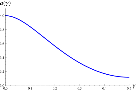
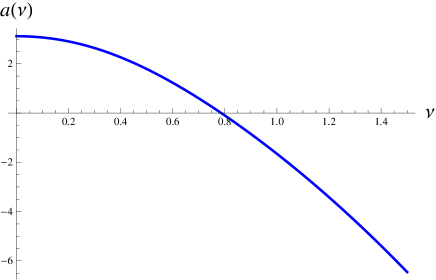
Fig. 2-a	Fig. 2-b

Figure 2: Function $a\left(\gamma\right)$ (solution to Eq. (2.18)) versus $\gamma$ (Fig. 2-a) and versus $\nu$ where $\gamma=\frac{1}{2}\,+\,i\,\nu$ (Fig. 2-b).

The Fourier image of $1/(p^{2}+m^{2})^{1-\gamma}$ in the coordinate representation is

$$\frac{1}{(\kappa+a)^{1-\gamma}}\xrightarrow{\mbox{\tiny Fourier image}}\frac{1}{\Gamma\left(1-\gamma\right)}\left(\frac{2\sqrt{a}}{r}\right)^{\gamma}\,K_{\gamma}\left(\sqrt{a}r\right)\,\xrightarrow{\sqrt{a}r\gg 1}\,\frac{1}{\Gamma\left(1-\gamma\right)}\left(\frac{2\sqrt{a}}{r}\right)^{\gamma}\sqrt{\frac{\pi}{2\sqrt{a}r}}\,e^{-\sqrt{a}r}$$ (2.19)

The function $1/(\kappa+a)^{1-\gamma}$ describes both the short distance (2.15) and long distance (2.17) behaviors. In [1] we demonstrated that the ground state with the minimal energy is reached with this class of functions.

2.2 Semi-classical approach: generalities

2.2.1 The method of steepest descent

For massless BFKL, a general solution has a form

$$\Psi\left(Y,\kappa\right)\,\,=\,\,\int^{\epsilon+i\infty}_{\epsilon-i\infty}\frac{d\gamma}{2\pi i}\,\phi_{in}\left(\gamma\right)\,e^{-E\left(\gamma\right)\,Y+\left(\gamma-1\right)\ln\kappa},$$ (2.20)

where $\phi_{in}\left(\gamma\right)$ should be found from the initial conditions at $Y=0$. For the massive case, we will look for solutions of Eq. (1.8) of the analogous form

$$\Psi\left(Y,l\right)\,\,=\,\,\int^{\epsilon+i\infty}_{\epsilon-i\infty}\frac{d\gamma}{2\pi i}\,\phi_{in}\left(\gamma\right)\,e^{-E\left(\gamma,l\right)\,Y+\left(\gamma-1\right)l},$$ (2.21)

where we introduced a new variable $l\,\,=\,\,\ln\left(\kappa+a\right)$, which is stable in the small-$\kappa$ limit, and $\phi_{in}\left(\gamma\right)$ is fixed by the initial conditions at $Y=0$. In Eq. (2.21) we can take the integral over $\gamma$ using the method of steepest descent, which is equivalent to a search of semiclassical solution to Eq. (1.8). The equation for the saddle point takes the general form

$$-\frac{\partial E\left(\gamma_{SP}\left(Y,l\right),l\right)}{\partial\gamma}\,Y\,+\,l\,=\,0.$$ (2.22)

If $\phi_{in}\left(\gamma\right)$ in the integrand of (2.21) is a smooth function, we can replace it with its value at $\gamma=\gamma_{SP}$. The integral over $\gamma$ in the vicinity of a saddle-point (2.22) yields

$$\Psi\left(Y,l\right)\,\,=$$ (2.23)

$$\,\,\phi_{in}\left(\gamma_{SP}\left(Y,l\right)\right)\,e^{-E\left(\gamma_{SP}\left(Y,l\right),l\right)\,Y+\left(\gamma_{SP}\left(Y,l\right)-1\right)l}\int^{\epsilon+i\infty}_{\epsilon-i\infty}\frac{d\gamma}{2\pi i}\,\exp\Big{(}-\frac{1}{2}\frac{\partial^{2}E\left(\gamma_{SP}\left(Y,l\right),l\right)}{\partial\gamma_{SP}^{2}}\,Y\left(\gamma-\gamma_{SP}\left(Y,l\right)\right)^{2}\Big{)}$$

$$=\phi_{in}\left(\gamma_{SP}\left(Y,l\right)\right)\,\sqrt{\frac{1}{2\pi\,\Big{|}\frac{\partial^{2}E\left(\gamma_{SP}\left(Y,l\right),l\right)}{\partial\gamma^{2}_{SP}}\Big{|}\,Y}}\,\,e^{S\left(Y,l\right)}\,\,=\,\,\phi_{in}\left(\gamma_{SP}\left(Y,l\right)\right)\,\sqrt{\frac{1}{2\pi\,\Big{|}\frac{\partial^{2}E\left(\gamma_{SP}\left(Y,l\right),l\right)}{\partial\gamma^{2}_{SP}}\Big{|}\,Y}}\,\,e^{-\frac{1}{2}l}\,e^{\omega_{eff}\left(l,Y\right)\,Y}.$$

The omission of higher-doer corrections in Eq. (2.23) is justified due to smallness of the parameter

$$R\,\,=\,\,\frac{1}{6}\Big{|}\frac{\partial^{3}E\left(\gamma_{SP}\left(Y,l\right),l\right)}{\partial\gamma_{SP}^{3}}\Big{|}\,Y\Bigg{/}\Big{(}\frac{1}{2}\Big{|}\frac{\partial^{2}E\left(\gamma_{SP}\left(Y,l\right),l\right)}{\partial\gamma^{2}_{SP}}\Big{|}\,Y\Big{)}^{3/2}\ll 1.$$ (2.24)

The smoothness of the initial function $\phi_{in}\left(\gamma\right)$ implies a condition

$$\frac{1}{\sqrt{\Big{|}\frac{1}{2}\frac{\partial^{2}E\left(\gamma_{SP}\left(Y,l\right),l\right)}{\partial\gamma^{2}_{SP}}\Big{|}\,Y}}\,\ll\,\frac{\ln\phi_{in}\left(\gamma\right)}{d\gamma}|_{\gamma=\gamma_{SP}}$$ (2.25)

and determines the kinematic region of applicability of the semiclassical approximation. As we will demonstrate below, both conditions are satisfied for sufficiently large $Y\,\gg\,1$.

2.2.2 Solution with method of characteristics

The method of characteristics for a partial differential equation (PDE) corresponds to a reduction of the PDEs

$$F(x_{1},\dots,x_{n},u,p_{1},\dots,p_{n})=0,\qquad p_{i}=\frac{\partial u}{\partial x_{i}}$$ (2.26)

to a system of ordinary differential equations (ODE) for characteristic lines along which the PDE converts into an ordinary differential equation. These characteristics satisfy the Lagrange-Charpit equations

$$\frac{\dot{x}_{i}}{F_{p_{i}}}=-\frac{\dot{p}_{i}}{F_{x_{i}}+F_{u}p_{i}}=\frac{\dot{u}}{\sum p_{i}F_{p_{i}}}.$$ (2.27)

A n instructive example familiar from a classical mechanics, is a Hamilton-Jacobi equation, for which the characteristic lines correspond to trajectories of particles which are solutions of the Newtonian equations of motion. A detailed discussion of the method is beyond the scope of the present paper and can be found in the literature (see e.g. textbooks  [22, 23]).

A direct application of the method of characteristics to the evolution equation Eq. (1.8) is not straightforward , since it is integrodifferential equation . However, as we will show below, for a special case which corresponds to a semiclassical approximation, this method is applicable. It is convenient to rewrite the wave function $\Psi$ in terms of the “action” $S$  [24],

$$\Psi(Y,\kappa)=e^{S(Y,\kappa)}.$$ (2.28)

Then the evolution equation Eq. (1.8) takes the form of a nonlinear PDE

$$F\left(Y,l,S,\,\gamma,\omega\right)\,\,=\,\,\omega\left(Y,l\right)\,-\,\chi\left(\gamma\left(Y,l\right)\right)\,\,-\,\,\widetilde{P}\left(l,\gamma\left(Y,l,a\right)\right)\,\,=\,\,0$$ (2.29)

where we introduced shorthand notations

$$\omega\left(Y,l\right)\,=\,\frac{\partial S\left(Y;l\right)}{\partial Y};~{}~{}~{}~{}\gamma\left(Y,l\right)\,-\,1\,=\,\frac{\partial S\left(Y;l\right)}{\partial l}~{}~{}~{}$$ (2.30)

and introduced a new variable $l\,\,=\,\,\ln\left(\kappa\,+\,a\right)$ which remains finite in the small-$\kappa$ limit. The explicit form of the function $\widetilde{P}\left(l,\gamma\left(Y,l,a\right)\right)$ in Eq. (2.30) will be specified below in section 2.4, here we will only mention that $\widetilde{P}\left(l,\gamma\left(Y,l,a\right)\right)\,\,\xrightarrow{l\,\gg\,1}\,\,0$. From the exact solutions of the massless BFKL 1.10, we expect that at large $\kappa$, the effective action should depend linearly on rapidity $Y$ and a new variable $l$,

$$S_{SC}\approx\omega_{\infty}+(\gamma_{\infty}-1)l,$$ (2.31)

where $\gamma_{\infty}$ and $\omega_{\infty}=\omega_{\rm BFKL}(\gamma_{\infty})$ are constants. In a semiclassical approximation which is valid for the moderate values of $Y$, we assume that $\omega_{SC}$ and $\gamma_{SC}$ are slowly varying functions of variables $l$, $Y$: viz. $\omega^{\prime}_{Y}\left(Y,l\right)\,\ll\,\omega^{2}\left(Y,l\right)$, $\omega^{\prime}_{l}\left(Y,l\right)\,\ll\,\omega^{2}\left(Y,l\right)$ and $\gamma^{\prime}_{Y}\left(Y,l\right)\,\ll\,\left(1-\gamma\left(Y,l\right)\right)^{2}$, $\gamma^{\prime}_{l}\left(Y,l\right)\,\ll\,\left(1-\gamma\left(Y,l\right)\right)^{2}$. Making this assumption, the equation Eq. (2.29) has a form of the PDE which can be solved using the method of characteristics  [22, 23]. The characteristic lines $l(t),Y(t),S(t)$, $\omega(t)$ and $\gamma_{SC}(t)$, where $t$ is some parameter (analog of time in case of classical mechanics), satisfy a system of ODEs:

$$(1.)\,\,\,\,\frac{dl}{d\,t}\,\,=\,\,\frac{\partial F}{\partial\gamma}\,\,=\,\,-\frac{d\chi\left(\gamma_{SC}\right)}{d\gamma_{SC}}\,\,-\,\,\frac{\partial\widetilde{P}\left(l(t),\gamma_{SC}(t),a\right)}{\partial\gamma_{SC}}$$ (2.32)

$$(2.)\,\,\,\,\,\,\,\frac{d\,Y\left(t\right)}{d\,t}\,\,=\,\,\frac{\partial F}{\partial\omega}\,\,=\,\,1\,\,\,\,\,\,\,$$

$$(3.)\,\,\,\,\frac{dS}{d\,t}\,\,=\,\,\left(\gamma-1\right)\,\frac{\partial F}{\partial\gamma}\,+\,\omega\,\frac{\partial F}{\partial\omega}\,\,=\,\,\,\,\left(\gamma_{SC}-1\right)\Big{\{}-\frac{d\chi\left(\gamma_{SC}\right)}{d\gamma}\,\,-\,\,\frac{\partial\widetilde{P}\left(l(t),\gamma_{SC}(t),a\right)}{\partial\gamma}\Big{\}}\,\,+\,\,\omega_{SC}$$

$$(4.)\,\,\,\,\frac{d\,\gamma_{SC}}{d\,t}\,\,=\,\,-\left(\,\frac{\partial F}{\partial l}\,+\,\left(\gamma_{SC}\,-\,1\right)\,\frac{\partial F}{\partial S}\,\right)\,\,=\,\,\frac{\partial\widetilde{P}\left(l(t),\gamma_{SC}(t),a\right)}{\partial\,l}$$

$$(5.)\,\,\,\,\frac{d\,\omega_{SC}}{d\,t}\,\,=\,\,-\left(\,\frac{\partial F}{\partial Y}\,+\,\omega\,\frac{\partial F}{\partial S}\,\right)\,\,=\,\,0$$

The second line of equation Eq. (2.32) implies that the parameter $t$ corresponds to a rapidity $Y$. From the fifth line of Eq. (2.32) we can see that $\omega_{SC}$ is conserved on characteristic lines, and can be fixed from the asymptotic conditions Eq. (1.10) as

$$\omega_{SC}\,\,=\,\,\chi\left(\gamma_{SC}\right)\,\,+\,\,\widetilde{P}\left(l(t),\gamma_{SC}(t),a\left(\gamma_{\infty}\right)\right)\,\,=\,\,\chi\left(\gamma_{\infty}\right).$$ (2.33)

A combination of Eq. (2.32)-4 and Eq. (2.32)-1 allows us to eliminate the $Y$-dependence, and find $\gamma_{SC}$ as a function of $l$ on a trajectory,

$$\frac{d\,\gamma_{SC}}{d\,l}\,\,=\,\,-\frac{\partial\widetilde{P}\left(l(t),\gamma_{SC}(t),a\right)}{\partial\,l}\Bigg{/}\left(\frac{d\chi\left(\gamma_{SC}\right)}{d\gamma_{SC}}\,\,+\,\,\frac{\partial\widetilde{P}\left(l(t),\gamma_{SC}(t),a\right)}{\partial\gamma_{SC}}\right)$$ (2.34)

Using Eq. (2.32)-1 we can write the equation for the trajectory $l=l\left(Y\right)$, which has the form

$$\frac{dl\left(Y\right)}{dY}\,\,=\,\,\,\,-\frac{d\chi\left(\gamma_{SC}\left(l\left(Y\right)\right)\right)}{d\gamma}\,\,-\,\,\frac{\partial\widetilde{P}\left(l(Y),\gamma_{SC}(l\left(Y\right)),a\right)}{\partial\gamma_{SC}}$$ (2.35)

The lines $l\left(Y\right)\,\equiv\,l_{SC}\left(Y\right)$ give the set of trajectories. The trajectory that leads to the dominant contribution to $\Psi\left(Y,l\right)$ can be found from the equation

$$l\,=\,l_{SC}\left(Y;\gamma_{\infty}\right)\,\,=\,\,l_{SP}\left(Y;\gamma_{\infty}\right)$$ (2.36)

Corresponding $\gamma_{SC}\left(Y,l_{SC}\left(Y\right);\gamma_{\infty}\right)\,=\,\gamma_{SP}\left(Y,l_{SP}\left(Y\right);\gamma_{\infty}\right)$. Finally, Eq. (2.32)-3 can be re-written in the form

$$\frac{dS}{d\,Y}\,\,=\,\,\left(\gamma_{SC}\left(Y,l\right)-1\right)\,\frac{dl\left(Y\right)}{dY}\,\,+\,\,\chi\left(\gamma_{SC}\left(Y,l\right)\right)\,\,+\,\,\widetilde{P}\left(l,\gamma_{SC}\left(Y,l,a\right)\right)$$ (2.37)

Comparing Eq. (2.32) with Eq. (2.23) one can see that the effective intercept is equal to $\omega_{eff}\left(Y,l\right)\,\,=\,\,\Big{(}S\left(Y,l_{SP}\left(Y\right)\right)\,+\,\frac{1}{2}\,l_{SP}\left(Y\right)\Big{)}/Y$.

Before applying the semiclassical approach to the BFKL equation for massive gluons, in the following subsection 2.3, we would like to test it on the massless BFKL equation (1), for which analytical solutions are known (see for example Ref. [3, 6]), and only after that in subsection 2.4 we apply it to the massive case.

2.3 Semi-classical approach: massless BFKL equation

For Eq. (1) $E\left(\gamma_{SP}\left(Y,l\right),l\right)\,=\,-\chi\left(\gamma\right)$ (see Eq. (1.10)). Combining this equation with Eq. (2.22), we obtain for the saddle point $\gamma_{SP}\left(Y,l=\ln\kappa\right)$

$$\chi^{\prime}_{\gamma}\left(\gamma_{SP}\left(\xi\right)\right)\,+\,\xi=0~{}~{}~{}~{}~{}~{}~{}\mbox{where}~{}~{}~{}~{}~{}~{}~{}\xi\,=\,l/Y.$$ (2.38)

The solution to Eq. (2.38) is shown in Fig. 3-a. From Eq. (2.23) one has that

$$\Psi_{\mbox{\tiny BFKL}}\left(Y,l=\ln\kappa\right)\,\,\propto\,\,e^{\omega_{eff}\left(\xi\right)Y},~{}~{}~{}~{}\mbox{where}~{}~{}~{}~{}~{}\omega_{eff}\left(\xi\right)\,\,=\,\,\chi\left(\gamma_{SP}\left(\xi\right)\right)\,+\,\left(\gamma_{SP}\left(\xi\right)-\frac{1}{2}\right)\xi.$$ (2.39)

The dependence $\omega_{eff}\left(\xi\right)$ is plotted in Fig. 3-b. The Fig. 3-c shows the ratio $R\left(\xi,Y\right)$ defined in Eq. (2.24). This ratio is small at large values of $Y$ and small $\xi$, thus justifying the applicability of semiclassical approximation in this region.

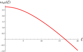
Fig. 3-a	Fig. 3-b	Fig. 3-c

Figure 3: Semi-classical solution for massless BFKL equation( see Eq. (1)): trajectories as function of $\xi=l/Y$ (Fig. 3-a); effective Pomeron intercept ($\omega_{eff}$ versus $\xi$ (Fig. 3-b); and the ratio $R$ of Eq. (2.24) at fixed $\xi$ as a function of $Y$(Fig. 3-c).

2.3.1 Diffusion approximation

As one can see from Fig. 3-a at $\xi\to 0$ or in other words, at large $Y\gg l$, the trajectory $\gamma_{SP}$ approaches a limiting value $\gamma_{SP}(\infty)=\frac{1}{2}$. Since $\chi(\gamma)$ is an analytic function near this point, it can be approximated by

$$\chi\left(\gamma\right)\,\,\,=\,\,\,\omega_{0}\,\,+\,\,D\,\left(\gamma-\frac{1}{2}\right)^{2}\,\,+\,\,{\cal O}\left(\left(\gamma-\frac{1}{2}\right)^{3}\right),$$ (2.40)

with $\omega_{0}=4\ln 2=2.772$   and   $D=14\zeta(3)=16.822$. In the approximation (2.40) the Eq. (2.38) can be solved easily and yields

$$\gamma_{SP}=\frac{1}{2}-\frac{\xi}{2D}.$$ (2.41)

Substituting (2.41) into Eq. (2.23), we obtain

$$\Psi{\mbox{\tiny BFKL}}\left(\xi,Y\right)\,=\,\phi_{in}\left(\frac{1}{2}-\frac{\xi}{2D}\right)\,\sqrt{\frac{1}{4\pi\,D\,Y}}\,\,e^{-\frac{1}{2}l}e^{\omega_{0}Y-\frac{\xi^{2}}{4DY}},$$ (2.42)

i.e., the semiclassical approach reproduces the diffusion approximation [6] for the BFKL equation.

2.3.2 Double log approximation

For small values of $\gamma\approx 0$, the BFKL kernel can be approximated by

$$\chi\left(\gamma\right)\,\,\,=\,\,\,\frac{1}{\gamma}.$$ (2.43)

In this limit, Eq. (2.38) gives the trajectory $\gamma_{SP}=1/\sqrt{\xi}$, and the wave function

$$\Psi_{\mbox{\tiny BFKL}}\left(\xi,Y\right)\,=\,\phi_{in}\left(1/\xi\right)\,\sqrt{\frac{1}{2\pi\,\xi^{3/2}\,Y}}\,\,e^{2\sqrt{\xi}Y}\,\,=\,\,\phi_{in}\left(Y/l\right)\,\sqrt{\frac{1}{2\pi\,l^{3/2}\,Y^{-1/2}}}\,\,e^{2\sqrt{Y\,l}}.$$ (2.44)

Eq. (2.44) is the solution in the double log approximation [6].

2.4 Semi-classical approach: kernels of the BFKL equation with massive gluon

Plugging the solution Eq. (2.21) into Eq. (1.8), we obtain the equation for $E\left(\gamma,l\right)$ in the form

$$E\left(\gamma,l\right)\,\, = \,\,T\left(e^{l}-a\right)\,\,+\,\,CT\left(l,\gamma\left(l\right),a;\right)\,\,-\,\,{\cal K}\left(l,\gamma\left(l\right),a\right),$$ (2.45)

where the emission kernel ${\cal K}\left(l,\gamma\left(l\right),a\right)$ is given by

$${\cal K}\left(l,\gamma\left(l\right),a\right)\,\,=\,\,\int^{1}_{\frac{a}{\kappa}}\frac{t^{\gamma\left(l\right)-1}\,dt}{\sqrt{(1-t)^{2}\,+\,\frac{2}{\kappa}(1+t)\,\,+\,\,\frac{1-4a}{\kappa^{2}}}}\,\,+\,\,\int^{1}_{0}\frac{t^{-\gamma\left(l\right)}\,dt}{\sqrt{(1-t)^{2}\,+\,\frac{2}{\kappa}t(1+t)\,\,+\,\,(1-4a)\frac{t^{2}}{\kappa^{2}}}}.$$ (2.46)

The integral over $t$ in Eq. (2.46) can be evaluated analytically and expressed in terms of the Appel function $F_{1}$:

$${\cal K}\left(l,\gamma\left(l\right),a\right) = 2\sqrt{\frac{t^{0}-t^{+}}{t^{+}-t^{-}}}\left(t^{+}\right)^{1-\gamma\left(l\right)}F_{1}\left(\frac{1}{2},1-\gamma\left(l\right),\frac{1}{2},\frac{1}{2},1-\frac{t^{0}}{t^{+}},\frac{t^{+}-t^{0}}{t^{+}-t^{-}}\right)$$

$$+ \sqrt{\pi}\,\,\frac{\Gamma\left(\gamma\left(l\right)\right)}{\Gamma\left(\frac{1}{2}+\gamma\left(l\right)\right)}{}_{2}F_{1}\left(\frac{1}{2},\frac{1}{2},\gamma\left(l\right)-\frac{1}{2},\frac{t^{+}}{t^{+}-t^{-}}\right)\,$$

$$+ \,\,B\left(1,\gamma\left(l\right)\right)\,F_{1}\left(\gamma\left(l\right),\frac{1}{2},\frac{1}{2},1+\gamma\left(l\right),t^{-},t^{+}\right),$$

where

$$t^{0}\,\,=\,\,\frac{a}{\kappa};~{}~{}~{}~{}~{}t^{\pm}\,\,=\,\,1\,+\,\frac{1}{\kappa}\,\,\,\pm\,\,\,2\,\sqrt{\frac{t^{0}\,-\,1}{\kappa}}.$$ (2.48)

For practical reasons it is convenient to introduce a function $P\left(l,\gamma,a\right)$ defined as

$$P\left(l,\gamma,a\right) = \int^{1}_{t^{0}}dt\left(t^{\gamma-1}-1\right)\Big{[}\frac{1}{\sqrt{(1-t)^{2}+(2/\kappa)\,(1+t)+(1-4a)/\kappa^{2}}}\,-\,\frac{1}{\sqrt{(1-t)^{2}}}\Big{]}\,\,-\,\,\int^{t^{0}}_{0}dt\frac{t^{\gamma-1}-1}{\sqrt{(1-t)^{2}}}$$ (2.49)

$$+ \int^{1}_{0}dt\left(t^{-\gamma}-1\right)\Big{[}\frac{1}{\sqrt{(1-t)^{2}\,+\,(2/\kappa)\,t(1+t)\,+\,(1-4a)\,t^{2}/\kappa^{2}}}\,-\,\frac{1}{\sqrt{(1-t)^{2}}}\Big{]}.$$

Then Eq. (2.45) can be cast into the form

$$E\,=\,-\chi\left(\gamma\left(l\right)\right)\,\,+\,\,\tilde{T}\left(l,a\right)\,\,+\,\,CT\left(l,\gamma\left(l\right),a\right)\,\,-\,\,P\left(l,\gamma\left(l\right),a\right)\,=\,-\chi\left(\gamma\left(l\right)\right)\,\,-\,\,\widetilde{P}\left(l,\gamma\left(l\right),a\right),$$ (2.50)

where

$$CT\left(l,\gamma,a\right)\,\,\, = \,\,\frac{5}{9}\frac{e^{(1-\gamma)\,l}}{e^{l}\,+1\,-a}\left(a-1\right)^{1+\gamma}B\left(\frac{a-1}{a},1-\gamma,a\right),$$ (2.51)

$$\tilde{T}\left(l,a\right)\,\, = \,\,T\left(e^{l}-a\right)\,\,-\,\,L\left(e^{l},a\right)$$ (2.52)

$$L\left(\kappa,a\right)\,\, = \,\,\int^{1}_{\frac{a}{\kappa}}\frac{dt}{\sqrt{(1-t)^{2}\,+\,\frac{2}{\kappa}(1+t)\,\,+\,\,\frac{1-4a}{\kappa^{2}}}}\,\,+\,\,\int^{1}_{0}\frac{dt}{\sqrt{(1-t)^{2}\,+\,\frac{2}{\kappa}t(1+t)\,\,+\,\,(1-4a)\frac{t^{2}}{\kappa^{2}}}}$$ (2.53)

$$= -\ln\left(1+a-\kappa+\sqrt{(1-a+\kappa)^{2}}\right)+\ln\left(1+\sqrt{1-4a+4\kappa}\right)-\frac{\kappa\ln\left(\kappa(1-\kappa+\sqrt{-4a+(1+\kappa)^{2}}\right)}{\sqrt{-4a+(1+\kappa)^{2}}}$$

$$+ \frac{\kappa\ln\left(1-4a+3\kappa+\sqrt{1-4a+4\kappa}\sqrt{-4a+(1+\kappa)^{2}}\right)}{\sqrt{-4a+(1+\kappa)^{2}}}$$

and $B\left(x,p,q\right)$ is the incomplete Beta function. Fig. 4 illustrates how all the ingredients of Eq. (2.50) behave as functions of $l=\ln(\kappa+a(\nu))$.

Fig. 4-a	Fig. 4-b	Fig. 4-c

Figure 4: All ingredients of Eq. (4) versus $l$ at $\gamma=\frac{1}{2}$ and $a=a\left(\frac{1}{2}\right)$ ( see Eq. (2.18) and Fig. 2).

3 Semi-classical solutions to the BFKL equation with massive gluon: numerical results

3.1 Trajectories and intercepts

For solving the general BFKL equation with massive gluons, we need to find the trajectory from Eq. (2.22) which will be a function of both $\xi=l/Y$ and $l$. According to the method of characteristics discussed in Section 2.2.2, these trajectories are the solutions of Eq. (2.33) or, equivalently, Eq. (2.34). Unfortunately, we are able to solve Eq. (2.33) only numerically, and these solutions are shown in Fig. 5.

Fig. 5-a	Fig. 5-b

Figure 5: The trajectories for the BFKL equation with massive gluons (solutions to Eq. (2.33) and to Eq. (2.35) ) versus $l\,=\,\ln\left(\kappa+a\right)$. Function $Y_{SC}\left(l\right)$ is the inverse function to $l=l_{SC}\left(Y\right)$ of Eq. (2.36).

All the trajectories can be characterized by their asymptotic boundary condition $\gamma_{SC}\left(l\right)\,\,\xrightarrow{l\,\gg\,1}\gamma_{\infty}$. We note that in Eq. (2.18) one should understand $\gamma$ as $\gamma_{\infty}$, thus reducing it to the form

$$T\left(-a\right)\,\,=\,\,-\,\,\chi\left(\gamma_{\infty}\right).$$ (3.54)

At small values of $l$ all the trajectories $\gamma_{SC}\left(l,\xi\right)$ vanish, reflecting the $K_{0}\left(\sqrt{a}r\right)$-behavior of the solution in the coordinate representation. The negative value of $\gamma_{SC}$ for soft $l$ in a numerical solution of Eq. (2.33) is different from what one expects from a massless BFKL. In section 3.4.3 we will discuss this region in more detail, here we only point out that $E\left(\gamma,l\right)$ is an analytical function of $\gamma$ for negative values of $\gamma$’s without any singularities at $\gamma=-n,n=0,1,2\dots$. Fig. 6 shows that $\gamma_{SP}\left(l\right)$ given by the solution of Eq. (2.33) and presented in Fig. 5, satisfy the equation even at $l\,<\,l_{soft}$.

Figure 6: Intercept of the massive BFKL Pomeron versus $l$ on the trajectories with different $\gamma_{\infty}$.

The trajectories $l_{SP}\left(Y\right)$ can be found by solving Eq. (2.36), and are shown in Fig. 5-b for several boundary conditions. In the $\xi\ll 1$ region the solution may be constructed analytically without solving an additional equation. The first observation is that at large $l$, the set of trajectories should coincide with the same set for the massless BFKL equations (2.38),

$$\gamma_{SP}\left(l,\xi\right)\,\xrightarrow{l\,\gg\,1}\,\gamma^{\mbox{\tiny BFKL}}_{SP}\left(\xi\right)\equiv\gamma_{\infty}.$$ (3.55)

Assuming that $\gamma^{\mbox{\tiny BFKL}}_{SP}\left(\xi\right)$ is close to $\frac{1}{2}$ at small $\xi$ (in so called Bjorken limit), we can consider a deviation as a small parameter,

$$\gamma_{SP}\left(l\right)\,\,=\,\,\gamma_{SC}\left(l,\gamma_{\infty}=\frac{1}{2}\right)\,\,+\,\,\delta\gamma_{SP}\left(l,\xi\right).$$ (3.56)

To find $\delta\gamma_{SP}\left(l,\xi\right)$, Eq. (2.22) can be re-written in the form

$$\delta\gamma_{SP}\left(l\right)\,=\,\lim_{\epsilon\to 0}\Bigg{(}-\xi\,\frac{\Big{(}\gamma_{SC}\left(l,\gamma_{\infty}=\frac{1}{2}\right)\,+\,\epsilon\,-\,\frac{1}{2}\Big{)}}{\Big{(}\frac{d\chi\left(\gamma=\gamma_{SC}\left(l,\gamma_{\infty}=\frac{1}{2}\right)\,+\,\epsilon\right)}{d\gamma}\,\,+\,\,\frac{\partial\widetilde{P}\left(l,\gamma=\gamma_{SC}\left(l,\gamma_{\infty}=\frac{1}{2}\right)+\,\epsilon,a\left(\gamma_{\infty}\right)\right)}{\partial\gamma}\Big{)}}\Bigg{)}$$ (3.57)

where $\epsilon\approx 0$ is a small cutoff needed to regularize some intermediate results. In particular, Eq. (3.57) reproduces Eq. (2.41) and gives the final result at $l\,\gg\,1$ where $\frac{d\chi\left(\gamma=\gamma_{SP}\left(l\right)\right)}{d\gamma}\,\,+\,\,\frac{\partial\widetilde{P}\left(l,\gamma=\gamma_{SC}\left(l\right),a\left(\gamma_{\infty}\right)\right)}{\partial\gamma}\,\,\ll\,\,1$.

The solution to Eq. (2.22) in this approximation has a form

$$\Psi\left(Y,l\right)\,\, = \,\phi_{in}\left(\gamma_{SP}\left(Y,l\right)\right)\,\sqrt{\frac{1}{2\pi\,\Big{|}\frac{\partial^{2}E\left(\gamma_{SP}\left(Y,l\right),l\right)}{\partial\gamma^{2}_{SP}}\Big{|}\,Y}}\,\,e^{-\frac{1}{2}l}\,\,e^{\omega_{eff}\left(l,\xi\right)Y},$$ (3.58)

where we introduced an effective intercept

$$\omega_{eff}\left(l,\xi\right)=-E\left(\gamma_{SP}\left(Y,l\right),l\right)+\left(\gamma_{SP}\left(Y,l\right)-\frac{1}{2}\right)\xi,$$ (3.60)

and $\gamma_{SP}$ is given by Eq. (3.56).

The $l$-dependence of the effective intercepts $\omega\left(l,\xi\right)$ is shown in Fig. 7. Note at small $\xi$, these intercepts are close to the massless BFKL given by Fig. 3-a in the entire region of $l$. In the region of large $\xi$, the effective intercepts are considerably smaller than the intercept of the massless BFKL Pomeron. For small $l$, i.e., the scattering amplitude at small values of $l$ and large values of $\xi$, is suppressed in comparison to the behavior determined by the intercept of the massless BFKL Pomeron. Since, the asymptotic region at high energies (large $Y$) corresponds to $\xi\,\ll\,1$, the high energy behavior of the massive BFKL Pomeron is the same as for the massless one. Therefore, we have the confirmation of our basic results of the numerical calculation (see Ref. [1]) in the framework of the semiclassical approach.

Fig. 7-a	Fig. 7-b

Figure 7: $\omega_{eff}\,\equiv\,\omega_{SP}$ of the massive BFKL Pomeron versus $l$ at fixed $\xi=l/Y$.Fig. 7-b illustrates that $\omega_{SP}\left(l\right)$ are close for small values of $\xi$.

3.2 Accuracy of the semiclassical approach

The accuracy of the semiclassical approximation is controlled by the ratio $R$ of Eq. (2.24). Fig. 8 shows this ratio for different values of $\xi$. From the figure we conclude that for $\xi\,\leq\,1$ the ratio $R$ is small and we can safely use the semiclassical approximation.

For $l<4$, the ratio $R$ is small in the region of large $Y$ (small $\xi$). The reason for this is since for large $l$, the solution of the BFKL equation for the massive gluons, should coincide with the solution of the massless BFKL equation.

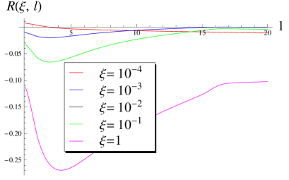
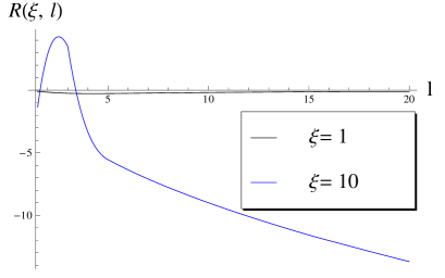
Fig. 8-a		Fig. 8-b

Figure 8: The ratio of Eq. (2.24) for large values of $Y$. Fig. 8-a shows this ratio at fixed $\xi=l/Y$ which are small, and Fig. 8-b presents $R$ at $\xi=1$ as a function of $l$.

These estimates confirm our expectation that the semiclassical method provides a reliable approach at high energies (large value of $Y$).

At large $\xi$, our procedure does not work even at large $l$. In terms of kinematics, we need to deal with $\gamma_{SC}\ll 1$, while in the Fig. 8 we used $\gamma_{SC}\,\xrightarrow{l\,\gg\,1}\,\frac{1}{2}$. For this region of large $l$ and $\xi$, we develop an approximation which corresponds to the double log approximation and for very large $l$ , and coincides with the DLA for the massless BFKL equation.

In Fig. LABEL:rsc we plot the ratio

$$R_{SC}\,\,=\,\,\frac{\frac{d\gamma_{SC}\left(l\right)}{dl}}{\left(1\,-\,\gamma_{SC}\left(l\right)\right)^{2}}.$$ (3.61)

This parameter controls the smoothness of the functions $\omega\left(Y,l\right)$ and $\gamma\left(Y,l\right)$, and thus a precision of the semiclassical approach. The Fig. LABEL:rsc shows that this ratio is very small at large $l$, and doesn’t exceed $\approx 0.4$ even at small $l$.

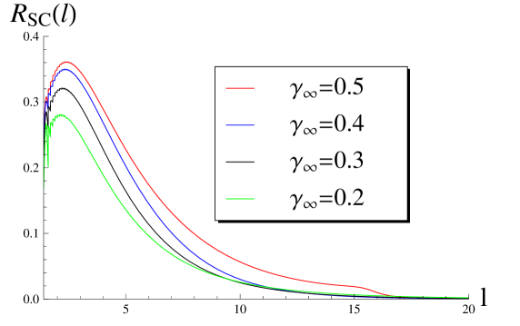
Figure 9: The ratio of Eq. (3.61) versus $l$. ˙rsc

3.3 Saturation momentum

It is well known that we can find a saturation momentum by searching for the particular trajectory on which the wave function $\Psi\left(Y,\kappa\right)=\mbox{const}$ (see Refs. [3, 25, 26]). Mathematically, this corresponds to a solution of a system of two equations

trajectory: $$-\frac{\partial E\left(\gamma_{SP}\left(Y,l\right),l\right)}{\partial\gamma}\,Y\,+\,l\,=\,0,$$

front line: $$E\left(\gamma_{SP}\left(Y,l\right),l\right)\,Y\,=\,(1-\gamma_{SP})\,l.$$ (3.62)

In the case of massless the BFKL equation, the solution to the equations of Eq. (3.3) is $\gamma_{SP}=\gamma_{cr}\,\,=\,\,0.37$  [3]. For the massive BFKL equation, the critical trajectory is shown in Fig. 10-a. The equation for the saturation momentum for massless BFKL equations of the form

$$l_{cr}\,\,=\,\,\ln\left(Q^{2}_{s}\left(Y\right)/Q^{2}_{s}\left(Y=0\right)\right)\,\,=\,\,\frac{\chi\left(\gamma_{cr}\right)}{1-\gamma_{cr}}\,Y.$$ (3.63)

The solution to Eq. (3.3) for $l_{cr}=\ln\left(Q^{2}_{s}\left(Y\right)/Q^{2}_{s}\left(Y=0\right)\right)$ is shown in Fig. 10-b. The difference between these two cases is sizable, only for small values of $l=\ln\left(\kappa+a\right)$.

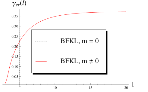
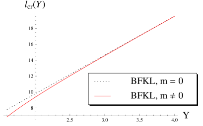
Fig. 10-a	Fig. 10-b

Figure 10: The critical trajectories for BFKL equation with $m=0$ and with $m\neq 0$ (see Fig. 10-a). Fig. 10-b shows the dependence of the saturation scale ($\ln\left(Q^{2}_{s}\left(Y\right)/Q^{2}_{s}\left(Y=0\right)\right)$) as function of $Y$.

3.4 Analytical solutions

In this section we develop two analytical methods of searching for solutions based on the diffusion and DLA approximations ,for the massless BFKL equation.

3.4.1 Diffusion approximation

A brief glance at the trajectories for small values of $\xi$ (see Fig. 6) allows us to conclude that these trajectories are close to $\gamma=\frac{1}{2}$ at least for $l\geq 5$. Therefore, for such values of $l$ we can develop the diffusion approach, in complete analogy with the case of massless BFKL equation, that has been discussed in section 2.3.1. In the vicinity of $\gamma=\frac{1}{2}$ we can expand the general expression of Eq. (2.50) as

$$\omega\left(\gamma,l\right)\,\,=\,\,-E\left(\gamma,l,a\right)\,\,=\,\,\Delta\left(l\right)\,\,+\,\,\Delta_{1}\left(l\right)\left(\gamma-\frac{1}{2}\right)\,\,+\,\,\Delta_{2}\left(l\right)\left(\gamma-\frac{1}{2}\right)^{2}.$$ (3.64)

Functions $\Delta\left(l\right),\Delta_{1}\left(l\right)$ and $\Delta_{2}\left(l\right)$ are plotted in Fig. 11-a.

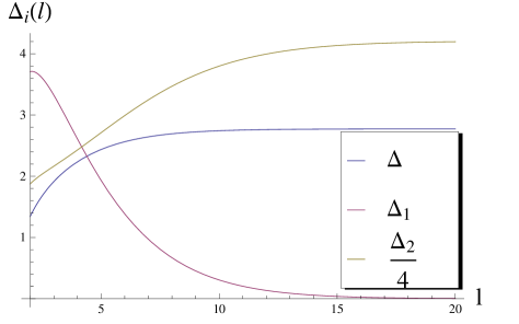
Fig. 11-a	Fig. 11-b

Figure 11: Functions $\Delta_{i}\left(l\right)$ of Eq. (3.64) (see Fig. 11-a) and functions $d_{i}\left(l\right)$ in Eq. (3.73) ( see Fig. 11-b)

We see that at large $l$ (say at $l\geq l_{0}\,\approx\,5$) the functions $\Delta_{i}$ reach constant values, $\Delta\left(l\right)\xrightarrow{l>l_{0}}\,\omega_{0}$; $\Delta_{1}\left(l\right)\xrightarrow{l>l_{0}}\,0$; and $\Delta_{2}\left(l\right)\xrightarrow{l>l_{0}}\,D$. Substituting expansion (3.64) into Eq. (2.33), we obtain

$$\Delta\left(l\right)\,+\,\Delta_{1}\left(l\right)\,\left(\gamma_{SC}\left(l\right)\,-\,\frac{1}{2}\right)\,\,+\,\,\Delta_{2}\left(l\right)\left(\gamma_{SP}-\frac{1}{2}\right)^{2}\,\,=\,\,\chi\left(\frac{1}{2}\right),$$ (3.65)

whose solution is

$$\gamma_{SC}\left(l\right)\,\,\equiv\,\,\gamma_{D}\left(l\right)\,\,=\,\,\left(-\Delta_{1}\left(l\right)\,\pm\,\sqrt{\Delta^{2}_{1}\left(l\right)\,-\,4\,\Delta_{2}\left(l\right)\left(\Delta\left(l\right)\,-\,\chi\left(\frac{1}{2}\right)\right)}\right){\Big{/}}\Big{(}2\,\Delta_{2}\left(l\right)\Big{)}.$$ (3.66)

The physical $\gamma_{D}$ corresponds to the minus sign in Eq. (3.66). In Fig. 12 we compare the trajectory Eq. (3.66) with the exact trajectory at $\xi=0.01$, that has been calculated in Section 3.1. For $l>l_{0}\sim 10$ we can safely use the solution Eq. (3.66).

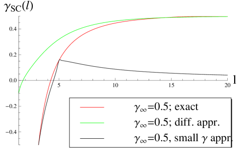
Figure 12: Functions $\gamma_{SC}\left(l,\xi\right)$ versus $l$: exact solution to Eq. (2.33); diffusion approximation and approximation at small values of $\gamma$. In the figure $\xi=0.01$.

Using Eq. (3.65), we can calculate the wave function of Eq. (2.23) which takes the form

$$\Psi\left(Y,l\right)\,\,=\,\,\phi_{in}\left(\gamma_{SP}\left(l\right)\right)\,\sqrt{\frac{1}{4\it\Delta_{2}\left(l\right)Y}}\,e^{-\frac{1}{2}l}\,e^{\omega_{eff}\left(l,\xi\right)\,Y},$$ (3.67)

with

$$\omega_{eff}\left(l,\xi\right)\,\,\,=\,\,\,\chi\left(\frac{1}{2}\right)\,\,-\,\,\frac{\left(\xi\left(\gamma_{D}\left(l\right)-\frac{1}{2}\right)\right)^{2}}{2\left(\Delta_{1}\left(l\right)+2\,\Delta_{2}\left(l\right)\,\left(\gamma_{D}\left(l\right)-\frac{1}{2}\right)\right)}.$$ (3.68)

The Eq. (3.68) provides a good description of the intercept for rather large $l\,>\,l_{0}\sim 10$.

3.4.2 Small $\gamma$ approximation

For $l\,<\,l_{0}$, we cannot use the diffusion approximation since, as we can see from Fig. 12, the diffusion trajectory is much larger than the exact one in this region. Actually, the exact $\gamma_{SP}\left(l,\xi\right)$ at small $\xi$ approaches $\gamma_{SP}\to 0$. At $\gamma\to 0$ the general expression for $P\left(l,\gamma,a\right)$ in Eq. (2.50) can be simplified and takes the form

$$\chi\left(\gamma\right)+\tilde{P}\left(l,\gamma,a\right)\,\,\xrightarrow{\gamma\to 0}\,\,\frac{1}{\gamma}+\tilde{P}_{\gamma\to 0}\left(l,\gamma,a\right)\,\,=\,\,\frac{1}{H\left(l,a\right)}\frac{1}{\gamma}\left(1-e^{-\gamma\left(l-l_{a}\right)}\right),$$ (3.69)

$$\mbox{with}~{}~{}~{}H\left(l,a\right)=\,1/\sqrt{\left(1\,+\,\exp\left(-l\right)\right)^{2}-4a\exp\left(-2l\right)}\,\,\,\,\mbox{and}~{}~{}~{}l_{a}=\ln a,$$

The Eq. (2.22) takes the form

$$\frac{1}{H\left(l,a\right)}\Big{\{}-\frac{1}{\gamma_{SC}^{2}}\left(1-e^{-\gamma_{SC}\left(l-l_{a}\right)}\right)\,+\,\left(l-l_{a}\right)\frac{1}{\gamma_{SC}}\,e^{-\gamma_{SC}\left(l-l_{a}\right)}\Big{\}}\,\,=\,\,-\,\,\xi.$$ (3.70)

The Eq. (3.70) has two solutions in different regions: (1) $\gamma\,\ll\,1$ but $\gamma\left(l-l_{a}\right)\,\gg\,1$; and (2) $\gamma\,\ll\,1$ and $\gamma\left(l-l_{a}\right)\,\ll\,1$.

In the first kinematic region Eq. (3.70) reduces to

$$-\frac{1}{\gamma_{SC}^{2}}\,\,=\,\,H\left(l,a\right),$$ (3.71)

with the solution

$$\gamma_{SC}\,\,=\,\,\sqrt{H\left(l,a\right)\,\xi}.$$ (3.72)

We can check that $\gamma\left(l-l_{a}\right)\,\,=\,\,\frac{1}{\sqrt{H\left(l,a\right)\,\xi}}\left(l-l_{a}\right)\xrightarrow{l\gg l_{a}}\,\sqrt{\frac{Y\,l}{H\left(l,a\right)}}\,\,\gg\,\,1.$ Therefore, this solution corresponds to the DLA approximation in this kinematic region.

For the kinematic region $\gamma\,\ll\,1$ and $\gamma\left(l-l_{a}\right)\,\ll\,1$ the Eq. (3.69) leads to the analytical function at $\gamma\to 0$ in contrast to the case of the massless BFKL kernel. Therefore, we can search for a parametrization $\omega\left(l,\xi\right)$, which has the same form as Eq. (3.65), viz.:

$$\omega_{\gamma\,\ll\,1}\left(\gamma,l\right)\,\,=\,\,-E\left(\gamma,l,a=4\right)\,\,=\,\,d\left(l\right)\,\,+\,\,d_{1}\left(l\right)\gamma\,\,+\,\,d_{2}\left(l\right)\,\gamma^{2},$$ (3.73)

with functions $d_{i}$ is plotted in Fig. 11-b. We can see from Fig. 12 that we can rely on Eq. (3.73) only for $l-l_{a}\ll 1/(\gamma=0.2)\approx 5$.

Eq. (2.22) with $\omega\left(l,\xi\right)$ given by Eq. (3.73), has a solution

$$\gamma_{SC}\left(l\right)\,\,\equiv\gamma_{S}\left(l\right)\,\,\equiv\,\,\gamma_{D}\left(l\right)\,\,=\,\,\left(-d_{1}\left(l\right)\,\pm\,\sqrt{d^{2}_{1}\left(l\right)\,-\,4\,d_{2}\left(l\right)\left(d\left(l\right)\,-\,\chi\left(\frac{1}{2}\right)\right)}\right){\Big{/}}\Big{(}2\,d_{2}\left(l\right)\Big{)}.$$ (3.74)

The solution (3.74) is shown in Fig. 12. This solution leads to good approximation for $l=3\div 5$ with

$$\omega_{eff}\left(l,\xi\right)\,\,\,\approx\,\,\,\chi\left(\frac{1}{2}\right)\,\,-\,\,\frac{\xi^{2}\,\gamma^{2}_{S}\left(l\right)}{2\left(d_{1}\left(l\right)+2\,d_{2}\left(l\right)\,\gamma_{S}\left(l\right)\right)}.$$ (3.75)

The wave function takes the form

$$\Psi\left(Y,l\right)\,\,=\,\,\phi_{in}\left(\gamma_{SP}\left(l\right)\right)\,\sqrt{\frac{1}{4\,d_{2}\left(l\right)Y}}\,e^{-l}\,e^{\omega_{eff}\left(l\right)\,Y}.$$ (3.76)

3.4.3 $l\,\leq\,l_{soft}$

Earlier we have seen that the trajectory $\gamma_{SP}(l)$ has a node at some value $l_{soft}$, and becomes even negative for $l\lesssim l_{soft}$. As we have seen earlier, the function $\omega_{SP}(\gamma)$ is analytic at $\gamma=0$, so we can extrapolate to negative but small $\gamma$’s using Eq. (3.73) (see Fig. 13). In principle, we can expect some high twists singularities at $\gamma=-n$ with $n=0,1,2,\dots$ which stem from the expansion of

$$\frac{1}{\sqrt{(1-t)^{2}+(2/\widetilde{\kappa})\,(1+t)+(1-4a)/\widetilde{\kappa}^{2}}}\,\,=\,\,\sum_{n=0}^{\infty}\,C_{n}\left(l,a\right)\,t^{n}$$ (3.77)

at small $t$ in Eq. (2.49). Taking the integral over $t$ in Eq. (2.49) in the vicinity of small $t$, one can see that for $\gamma\to-n$ we obtain the same expression as in Eq. (3.69), replacing $\gamma$ in Eq. (3.69) by $\gamma+n$. The energy (intercept) turns out to be a regular function at $\gamma=-n$, and we can use Eq. (3.73) for $|\gamma+1|\,<\,1$ with function $d^{(1)}_{i}\left(l\right)$ calculated at $\gamma=-1$ ( see Fig. 12 and Fig. 13).

Fig. 13 illustrates that the intercept $\omega\left(\gamma,l\right)$ is the analytical function without singularities at negative $\gamma$ which increases at large $|\gamma|$.

Figure 13: Function $\omega\left(\gamma,l\right)$ versus $\gamma$ at fixed $l$. $\omega_{BFKL}\,\,=\,\,\chi\left(\frac{1}{2}\right)$.

Unfortunately, we have not found a simple analytical approach that is able to describe the scattering amplitude at all values of $l$. However, we would like to recall that the numerical solutions to Eq. (3.56) and Eq. (3.57) depend neither on the value of the QCD coupling, nor on the initial condition, and reduce the procedure of calculation of the scattering amplitude to a simple equation. Solving this equation is much easier task than the exact numerical calculation of the eigenvalues and eigenfunctions that was done in Ref. [1].

4 Conclusions

In our previous paper (see Ref. [1]) we studied the BFKL equation with massive gluons in the lattice and proved that its spectrum coincides with the spectrum of the massless BFKL equation. This observation gives rise to a hope that the correct large impact parameter ($b$) behavior of the scattering amplitude $A\propto\exp\left(-mb\right)$, which is the inherent feature of the massive BFKL equation, will not affect the high energy behavior of the scattering amplitude. Therefore, we can expect that the modification of the BFKL equation due to confinement would not affect strongly the main equations that govern the physics at high energy ( in particular, the non-linear equations of the CGC/saturation approach to high density QCD).

In this paper we developed the semiclassical approximation which allowed us to investigate the high energy behavior of the scattering amplitude. The method provides a simple procedure for the calculation and reduces it to a numerical solution of Eq. (2.33), which is much simpler than the direct numerical calculations of the eigenvalue problem in the lattice realized in Ref. [1].

Having these solutions, we propose a modification of high energy asymptotic behavior, caused by the correct large $b$ exponential fall off of the amplitude. Actually, we did not find any unexpected behavior, and the semiclassical solution reproduces the scattering amplitude which is very close to the amplitude of the massless BFKL equation, at least at high energies.

In section 3.3 we estimate the value of the saturation momentum, solving the linear evolution equation with very general assumptions about the non-linear corrections. We demonstrated that the value of the saturation momentum is close to the one for the massless BFKL equations, leading to the assumption that saturation physics will look similar for both massive and massless BFKL equations.

We believe that in this paper we taken the natural next step in the understanding of the influence of the correct large $b$ decrease of the amplitude on its high energy behavior. It should be stressed that this behavior is interesting as it provides the high energy amplitude for the electroweak-weak theory, which can be measured experimentally. The solution which has been discussed in this paper, determines the asymptotic high energy behavior of the electroweak-weak theory for zero Weinberg angle. We plan to address the physical case of nonzero Weinberg angle [2] elsewhere.

5 Acknowledgements

We thank our colleagues at UTFSM and Tel Aviv university for encouraging discussions. This research was supported by the BSF grant 2012124 and by the Fondecyt (Chile) grants 1140842 and 1140377.

References

- [1] E. Levin, L. Lipatov and M. Siddikov, Phys. Rev. D 89 (2014) 074002 [arXiv:1401.4671 [hep-ph]].
- [2] J. Bartels, L. N. Lipatov and K. Peters, Nucl. Phys. B 772 (2007) 103 [hep-ph/0610303].
- [3] L. V. Gribov, E. M. Levin and M. G. Ryskin, Phys. Rep. 100 (1983) 1.
- [4] A. H. Mueller and J. Qiu, Nucl. Phys. B268 (1986) 427.
-
[5]
L. McLerran and R. Venugopalan,
Phys. Rev. D49 (1994) 2233, 3352; D50 (1994) 2225;
D53 (1996) 458;
D59 (1999) 094002. - [6] Yuri V Kovchegov and Eugene Levin, “ Quantum Choromodynamics at High Energies”, Cambridge Monographs on Particle Physics, Nuclear Physics and Cosmology, Cambridge University Press, 2012 and references therein.
- [7] A. Kovner and U. A. Wiedemann, Phys. Rev. D 66, 051502 (2002) [hep-ph/0112140].
- [8] A. Kovner and U. A. Wiedemann, Phys. Rev. D 66, 034031 (2002) [hep-ph/0204277].
- [9] A. Kovner and U. A. Wiedemann, Phys. Lett. B 551, 311 (2003) [hep-ph/0207335].
- [10] E. Ferreiro, E. Iancu, K. Itakura and L. McLerran, Nucl. Phys. A 710, 373 (2002) [hep-ph/0206241].
-
[11]
M. Froissart,
Phys. Rev. 123 (1961) 1053;
A. Martin, “Scattering Theory: Unitarity, Analitysity and Crossing.” Lecture Notes in Physics, Springer-Verlag, Berlin-Heidelberg-New-York, 1969. - [12] V. N. Gribov, Nucl. Phys. B 139, 1 (1978).
- [13] J. Serreau, M. Tissier and A. Tresmontant, Phys. Rev. D 89, 125019 (2014) [arXiv:1307.6019 [hep-th]] J. Serreau and M. Tissier, Phys. Lett. B 712, 97 (2012) [arXiv:1202.3432 [hep-th]];
- [14] N. Vandersickel and D. Zwanziger, Phys. Rept. 520, 175 (2012) [arXiv:1202.1491 [hep-th]] and references therein.
- [15] J. M. Cornwall, Mod. Phys. Lett. A 28, 1330035 (2013) [arXiv:1310.7897 [hep-ph]]; J. A. Gracey, arXiv:1409.0455 [hep-ph].
- [16] P. J. Silva, D. Dudal and O. Oliveira, “Spectral densities from the lattice,” arXiv:1311.3643 [hep-lat]. P. J. Silva, O. Oliveira, D. Dudal, P. Bicudo and N. Cardoso, b“Many faces of the Landau gauge gluon propagator at zero and finite temperature: positivity violation, spectral density and mass scales,” PoS QCD -TNT-III, 040 (2013) [arXiv:1401.1554 [hep-lat]].
- [17] E. A. Kuraev, L. N. Lipatov, and F. S. Fadin, Sov. Phys. JETP 45, 199 (1977); Ya. Ya. Balitsky and L. N. Lipatov, Sov. J. Nucl. Phys. 28, 822 (1978).
- [18] L. N. Lipatov, Phys. Rep. 286 (1997) 131; Sov. Phys. JETP 63 (1986) 904 [Zh. Eksp. Teor. Fiz. 90, 1536 (1986)].
- [19] I. Balitsky, Nucl. Phys. B463 99 (1996); e-Print Archive: hep-ph/9509348; Phys. Rev. Lett. 81 2024 (1998); e-Print Archive: hep-ph/9807434; Phys. Rev.D60 014020 (1999); Y. V. Kovchegov, Phys. Rev. D 61, 074018 (2000) [arXiv:hep-ph/9905214].
- [20] J. Jalilian Marian, A. Kovner, A.Leonidov and H. Weigert, Nucl. Phys.B504 415 (1997); e-Print Archive: hep-ph/9701284 Phys. Rev. D59 014014 (1999); e-Print Archive: hep-ph/9706377 J. Jalilian Marian, A. Kovner and H. Weigert, Phys. Rev.D59 014015 (1999); e-Print Archive: hep-ph/9709432; A. Kovner and J.G. Milhano, Phys. Rev. D61 014012 (2000) . e-Print Archive: hep-ph/9904420. A. Kovner, J.G. Milhano and H. Weigert, Phys.Rev. D62 114005 (2000); H. Weigert, Nucl.Phys. A 703 (2002) 823; E.Iancu, A. Leonidov and L. McLerran, Nucl. Phys. A 692 (2001) 583; Phys. Lett. B 510 (2001) 133; E. Ferreiro, E. Iancu, A. Leonidov, L. McLerran; Nucl. Phys.A703 (2002) 489.
- [21] I. Gradstein and I. Ryzhik, Table of Integrals, Series, and Products, Fifth Edition, Academic Press, London, 1994.
- [22] F. John, “Partial Differential Equations”, Springer, New York 1971.
- [23] E. Kamke, “Differentialgleichungen Lösungsmethoden und Lösungen”, Vieweg+Teubner Verlag, Leipzig 1959.
- [24] R. Feynman, P. Hibbs, “Quantum Mechanics and Path Integrals”, McGraw-Hill, New York, 1965
- [25] A. H. Mueller and D. N. Triantafyllopoulos, Nucl. Phys. B640 (2002) 331 [arXiv:hep-ph/0205167]; D. N. Triantafyllopoulos, Nucl. Phys. B648 (2003) 293 [arXiv:hep-ph/0209121].
- [26] S. Munier and R. B. Peschanski, Phys. Rev. D 70 (2004) 077503 [arXiv:hep-ph/0401215]; Phys. Rev. D 69 (2004) 034008 [arXiv:hep-ph/0310357]; Phys. Rev. Lett. 91 (2003) 232001 [arXiv:hep-ph/0309177].