Existence and non-existence results for the $\displaystyle SU(3)$ singular Toda system on compact surfaces

Abstract

We consider the $\displaystyle SU(3)$ singular Toda system on a compact surface $\displaystyle(\Sigma,g)$

$$\left\{\begin{array}[]{l}-\Delta u_{1}=2\rho_{1}\left(\frac{h_{1}e^{u_{1}}}{\int_{\Sigma}h_{1}e^{u_{1}}\mathrm{d}V_{g}}-1\right)-\rho_{2}\left(\frac{h_{2}e^{u_{2}}}{\int_{\Sigma}h_{2}e^{u_{2}}\mathrm{d}V_{g}}-1\right)-4\pi\sum_{m=1}^{M}\alpha_{1m}\left(\delta_{p_{m}}-1\right)\\ -\Delta u_{2}=2\rho_{2}\left(\frac{h_{2}e^{u_{2}}}{\int_{\Sigma}h_{2}e^{u_{2}}\mathrm{d}V_{g}}-1\right)-\rho_{1}\left(\frac{h_{1}e^{u_{1}}}{\int_{\Sigma}h_{1}e^{u_{1}}\mathrm{d}V_{g}}-1\right)-4\pi\sum_{m=1}^{M}\alpha_{2m}\left(\delta_{p_{m}}-1\right)\end{array}\right.,$$

where $\displaystyle h_{i}$ are smooth positive functions on $\displaystyle\Sigma$, $\displaystyle\rho_{i}\in\mathbb{R}_{+}$, $\displaystyle p_{m}\in\Sigma$ and $\displaystyle\alpha_{im}>-1$.
We give both existence and non-existence results under some conditions on the parameters $\displaystyle\rho_{i}$ and $\displaystyle\alpha_{im}$. Existence results are obtained using variational methods, which involve a geometric inequality of new type; non-existence results are obtained using blow-up analysis and localized Pohožaev-type identities.

1 Introduction

Let $\displaystyle\Sigma$ be a closed surface and $\displaystyle g$ be a Riemannian metric on $\displaystyle\Sigma$. Consider the following system on $\displaystyle\Sigma$:

$$-\Delta u_{i}=\sum_{j=1}^{2}a_{ij}\rho_{j}(h_{j}e^{u_{j}}-1)-4\pi\sum_{m=1}^{M}\alpha_{im}(\delta_{p_{m}}-1),\quad\quad\quad i=1,2,$$ (1)

where $\displaystyle\Delta=\Delta_{g}$ is the Laplace-Beltrami operator, $\displaystyle\rho_{i}$ are positive parameters, $\displaystyle h_{i}$ are smooth positive functions on $\displaystyle\Sigma$, $\displaystyle\alpha_{im}$ are real numbers greater than $\displaystyle-1$, $\displaystyle p_{m}$ are given points of $\displaystyle\Sigma$, and $\displaystyle A=(a_{ij})_{ij}$ is the Cartan matrix of $\displaystyle SU(3)$

$$\left(\begin{array}[]{cc}2&-1\\ -1&2\end{array}\right).$$

System (1) is known as the $\displaystyle SU(3)$ singular Toda system. Together with its $\displaystyle N\times N$ extension, it has been widely studied in literature due to its important role in both geometry and mathematical physics. In geometry, it appears in the description of holomorphic curves in $\displaystyle\mathbb{C}\mathbb{P}^{3}$ (see e.g. [10, 17, 9]), while in mathematical physics it arises in the non-abelian Chern-Simons theory (see [19, 42, 38]). The singularities represent respectively the ramification points of the complex curves and the vortices of the wave functions.

To better understand this system, it is convenient to re-write it in an equivalent form. Let $\displaystyle G_{p}$ be the Green function of $\displaystyle-\Delta$ centered at a point $\displaystyle p\in\Sigma$, namely the solution of

$$\left\{\begin{array}[]{l}-\Delta G_{p}=\delta_{p}-1\\ \int_{\Sigma}G_{p}\mathrm{d}V_{g}=0\end{array}\right..$$

Consider now the substitution $\displaystyle u_{i}\mapsto u_{i}+4\pi\sum_{m=1}^{M}\alpha_{im}G_{p_{m}}$: the newly-defined $\displaystyle u=(u_{1},u_{2})$ solves

$$\left\{\begin{array}[]{l}-\Delta u_{1}=2\rho_{1}\left(\widetilde{h}_{1}e^{u_{1}}-1\right)-\rho_{2}\left(\widetilde{h}_{2}e^{u_{2}}-1\right)\\ -\Delta u_{2}=2\rho_{2}\left(\widetilde{h}_{2}e^{u_{2}}-1\right)-\rho_{1}\left(\widetilde{h}_{1}e^{u_{1}}-1\right)\end{array}\right.,$$

where the new functions $\displaystyle\widetilde{h}_{i}$ have the expression

$$\widetilde{h}_{i}:=h_{i}e^{-4\pi\sum_{m=1}^{M}\alpha_{im}G_{p_{m}}}\quad\quad\quad i=1,2$$

and verify

$$\widetilde{h}_{i}\in C^{\infty}\left(\Sigma\setminus\{p_{1},\dots,p_{M}\}\right)\quad\quad\quad\widetilde{h}_{i}|_{\Sigma\setminus\{p_{1},\dots,p_{M}\}}>0\quad\quad\quad\widetilde{h}_{i}\sim d(\cdot,p_{m})^{2\alpha_{im}}\quad\text{near }p_{m}.$$ (2)

Integrating by parts over the whole $\displaystyle\Sigma$, we deduce

$$\int_{\Sigma}\widetilde{h}_{1}e^{u_{1}}\mathrm{d}V_{g}=\int_{\Sigma}\widetilde{h}_{1}e^{u_{2}}\mathrm{d}V_{g}=1,$$

therefore the system is equivalent to

$$\left\{\begin{array}[]{l}-\Delta u_{1}=2\rho_{1}\left(\frac{\widetilde{h}_{1}e^{u_{1}}}{\int_{\Sigma}\widetilde{h}_{1}e^{u_{1}}\mathrm{d}V_{g}}-1\right)-\rho_{2}\left(\frac{\widetilde{h}_{2}e^{u_{2}}}{\int_{\Sigma}\widetilde{h}_{2}e^{u_{2}}\mathrm{d}V_{g}}-1\right)\\ -\Delta u_{2}=2\rho_{2}\left(\frac{\widetilde{h}_{2}e^{u_{2}}}{\int_{\Sigma}\widetilde{h}_{2}e^{u_{2}}\mathrm{d}V_{g}}-1\right)-\rho_{1}\left(\frac{\widetilde{h}_{1}e^{u_{1}}}{\int_{\Sigma}\widetilde{h}_{1}e^{u_{1}}\mathrm{d}V_{g}}-1\right)\end{array}\right.,$$ (3)

Problem (3) admits a variational formulation, that is its solutions are critical points of the following energy functional defined on $\displaystyle H^{1}(\Sigma)^{2}$:

$$J_{\rho}(u):=\int_{\Sigma}Q(u)\mathrm{d}V_{g}-\sum_{i=1}^{2}\rho_{i}\left(\log\int_{\Sigma}\widetilde{h}_{i}e^{u_{i}}\mathrm{d}V_{g}-\int_{\Sigma}u_{i}\mathrm{d}V_{g}\right).$$ (4)

Here, $\displaystyle Q(u)$ is given by

$$Q(u)=\frac{|\nabla u_{1}|^{2}+\nabla u_{1}\cdot\nabla u_{2}+|\nabla u_{2}|^{2}}{3},$$

$\displaystyle\nabla=\nabla_{g}$ is the gradient given by the metric $\displaystyle g$ and $\displaystyle\cdot$ denotes the Riemannian scalar product.
To study the properties of the functional $\displaystyle J_{\rho}$, a basic tool is the Moser-Trudinger inequality, which was proved in [7, 4] (and, for the regular case, in [25]).

$$4\pi\sum_{i=1}^{2}\min\left\{1,1+\min_{m}\alpha_{im}\right\}\left(\log\int_{\Sigma}\widetilde{h}_{i}e^{u_{i}}\mathrm{d}V_{g}-\int_{\Sigma}u_{i}\mathrm{d}V_{g}\right)\leq\int_{\Sigma}Q(u)\mathrm{d}V_{g}+C.$$ (5)

As a consequence, $\displaystyle J_{\rho}$ is bounded from below as long as $\displaystyle\rho_{i}\leq 4\pi\min\left\{1,1+\min_{m}\alpha_{im}\right\}$ for both $\displaystyle i=1,2$. Moreover, if both parameters are strictly smaller than these thresholds, the functional is coercive in the space of functions with zero average; there will be no loss of generality in restricting the problem to this space, since both (3) and (4) are invariant by addition of constants. Hence, in this case we get minimizing solutions.

If one (or both) of the $\displaystyle\rho_{i}$ is allowed to attain greater values, then one can build suitable test functions to show that the energy functional is unbounded from below, as was done in the same papers where (5) is proved. Therefore, one can no longer use minimization techniques to find critical points. However it is possible to prove that when the Euler-Lagrange energy (4) becomes largely negative at least one of the functions $\displaystyle\widetilde{h}_{i}e^{u_{i}}$ has to concentrate near a finite number of points. One can eventually derive existence results out of this statement using min-max or Morse theory.

To describe in more detail the situation we first consider Liouville’s equation, that is the scalar counterpart of (3):

$$-\Delta u=2\rho\left(\frac{he^{u}}{\int_{\Sigma}he^{u}\mathrm{d}V_{g}}-1\right)-4\pi\sum_{m=1}^{M}\alpha_{m}(\delta_{p_{m}}-1).$$

Through a change of variable similar to that before (3), this is equivalent to

$$-\Delta u=2\rho\left(\frac{\widetilde{h}e^{u}}{\int_{\Sigma}\widetilde{h}e^{u}\mathrm{d}V_{g}}-1\right).$$ (6)

with $\displaystyle\widetilde{h}$ having the same behavior as in (2) around singular points.
Liouville’s equation has also great importance in geometry and mathematical physics: it appears in the problem of prescribing the Gaussian curvature on surfaces with conical singularities and in models from abelian Chern-Simons theory. This problem has also been very much studied in literature, with many results concerning existence of solutions, compactness properties, blow-up analysis et al., which have been summarized e.g. in the reviews [31, 39].

(6) is the Euler-Lagrange equation for the functional

$$I_{\rho}(u):=\frac{1}{2}\int_{\Sigma}|\nabla u|^{2}\mathrm{d}V_{g}-2\rho\left(\log\int_{\Sigma}\widetilde{h}e^{u}\mathrm{d}V_{g}-\int_{\Sigma}u\mathrm{d}V_{g}\right).$$ (7)

The classical Moser-Trudinger inequality and its extension to the singular cases ([35, 20, 15, 40]) yield boundedness from below of $\displaystyle I_{\rho}$ if and only if $\displaystyle\rho\leq 4\pi\min\left\{1,1+\min_{m}\alpha_{m}\right\}$ and coercivity if and only if $\displaystyle\rho$ is strictly smaller than this value.

For larger values of $\displaystyle\rho$, despite the lack of lower bounds on the energy $\displaystyle I_{\rho}$, it is however possible to prove that functions with low energy must concentrate near finitely-many points. A heuristic reason for this fact goes as follows: the Moser-Trudinger inequality can be localized on any region of $\displaystyle\Sigma$ via cut-off functions, see [16]. A consequence of this fact is that functions that are spread over $\displaystyle\Sigma$ satisfy a Moser-Trudinger inequality with an improved constant, which favors lower bounds on $\displaystyle I_{\rho}$. Hence, if lower bounds fail, $\displaystyle u$ should concentrate rather than spread.
Notice that when all the $\displaystyle\alpha_{j}$’s are negative the localized Moser-Trudinger constant near a singular point $\displaystyle p_{i}$ is $\displaystyle 4\pi(1+\alpha_{i})$, while near a regular point it is simply $\displaystyle 4\pi$. Based on these considerations, in [12] the following weighted cardinality $\displaystyle\omega_{\underline{\alpha}}$ on finite sets was introduced:

$$\omega_{\underline{\alpha}}(\{x\}):=\left\{\begin{array}[]{ll}1+\alpha_{m}&\text{if }x=p_{m}\\ 1&\text{if }x\not\in\{p_{1},\dots,p_{M}\}\end{array}\right.\quad\quad\quad\omega_{\underline{\alpha}}\left(\bigcup_{k}\{x_{k}\}\right):=\sum_{k}\omega_{\underline{\alpha}}(\{x_{k}\});$$ (8)

and it was shown that if a function $\displaystyle u$ has low energy, then the normalized measure $\displaystyle\widetilde{h}e^{u}$ must distributionally approach the following set of measures (appeared also in [18])

$$\Sigma_{\rho,\underline{\alpha}}:=\left\{\sum_{x_{k}\in\mathcal{J}}t_{k}\delta_{x_{k}}:\,x_{k}\in\Sigma,\,t_{k}\geq 0,\,\sum_{x_{k}\in\mathcal{J}}t_{k}=1,\,4\pi\omega_{\underline{\alpha}}(\mathcal{J})<\rho\right\}.$$

Using variational methods, a compactness result in [3] and a monotonicity argument in [37] it was also shown that, endowing $\displaystyle\Sigma_{\rho,\underline{\alpha}}$ with the weak topology of distributions, solutions to (6) (up to a discrete set of $\displaystyle\rho$’s, for compactness reasons) exist provided $\displaystyle\Sigma_{\rho,\underline{\alpha}}$ is non-contractible. We notice that the problem is not always solvable, as in the classical case of the teardrop: the sphere with only one singular point. Sufficient and necessary conditions for contractibility were given in [11].
The case of positive singularities was treated in [1] on surfaces with positive genus. There are some other existence results ([2, 33]) which also work for the case of the sphere or of the real projective plane. We also refer to [14] for the derivation of a degree-counting formula.

We turn now to system (3): for the regular case some existence results were found in [32] ($\displaystyle\rho_{1}<4\pi$ and $\displaystyle\rho_{2}\not\in 4\pi\mathbb{N}$), in [34] ($\displaystyle\rho_{i}\in(4\pi,8\pi)$), [23] ($\displaystyle\rho_{1}\in(4\pi,8\pi)$ and $\displaystyle\rho_{2}\not\in 4\pi\mathbb{N}$) and in [6] ($\displaystyle\Sigma$ of positive genus and $\displaystyle\rho_{i}\not\in 4\pi\mathbb{N}$). In the latter paper, with a construction related to that in [1], the case of positive singular weights was also treated while in [5], still for positive genus, some cases with negative coefficients $\displaystyle\alpha_{im}$ were discussed.

The above reasoning for the scalar singular equation allows to prove a related alternative for the two components of the system. If we use the compact notation $\displaystyle\underline{\alpha}_{1}:=(\alpha_{11},\dots,\alpha_{1m}),\,\underline{\alpha}_{2}:=(\alpha_{21},\dots,\alpha_{2m})$, then it turns out that for $\displaystyle J_{\rho}(u)$ low either $\displaystyle\widetilde{h}_{1}e^{u_{1}}$ is distributionally close to $\displaystyle\Sigma_{\rho_{1},\underline{\alpha}_{1}}$ or $\displaystyle\widetilde{h}_{2}e^{u_{2}}$ is close to $\displaystyle\Sigma_{\rho_{2},\underline{\alpha}_{2}}$. To express this (non-exclusive) alternative, it is natural introduce the join of two topological spaces $\displaystyle X$ and $\displaystyle Y$ (see for instance [22]):

$$X\star Y:=\frac{X\times Y\times[0,1]}{\sim},$$ (9)

where $\displaystyle\sim$ is the equivalence relation among triples $\displaystyle(x,y,t)$ given by

$$(x,y,0)\sim(x,y^{\prime},0)\quad\forall\,x\in X,\,\forall\,y,y^{\prime}\in Y\quad\quad\quad(x,y,1)\sim(x^{\prime},y,1)\quad\forall\,x,x^{\prime}\in X,\,\forall\,y\in Y.$$

The join of $\displaystyle\Sigma_{\rho_{1},\underline{\alpha}_{1}}$ and $\displaystyle\Sigma_{\rho_{2},\underline{\alpha}_{2}}$ could then be used to characterize low-energy levels of $\displaystyle J_{\rho}$, with the join parameter $\displaystyle s\in[0,1]$ expressing whether $\displaystyle\widetilde{h}_{1}e^{u_{1}}$ is closer to $\displaystyle\Sigma_{\rho_{1},\underline{\alpha}_{1}}$ or $\displaystyle\widetilde{h}_{2}e^{u_{2}}$ is closer to $\displaystyle\Sigma_{\rho_{2},\underline{\alpha}_{2}}$ (for example $\displaystyle s=\frac{1}{2}$ would describe couples with the same scale of concentration).
This description is however not optimal in general, as it does not take accurately into account the interaction between two components $\displaystyle u_{1}$ and $\displaystyle u_{2}$. For the regular case of (3), in [34] it was shown that the relative rate of concentration of the two components plays a role in this matter.
More precisely, it was shown that if $\displaystyle u_{1},u_{2}$ concentrate near the same point and with the same scale (see Section 2 for a more precise definition of the latter), then the Moser-Trudinger constants for the system double. As a consequence of this fact it turns out that, when $\displaystyle\rho_{1},\rho_{2}\in(4\pi,8\pi)$ and no singularities occur, then join elements of the form $\displaystyle\left(x,x,\frac{1}{2}\right)$, $\displaystyle x\in\Sigma$ have to be excluded (see [23] for higher values of $\displaystyle\rho_{1}$).

One of the main goals of this paper is to show a new improved inequality for the singular system (3), in order to understand at the same time the effect of the interaction of the two components among themselves and with the singularities. We prove in particular (see Section 5) that if the two components are concentrated near the same singular point with the same rate, coercivity of the Euler-Lagrange energy holds provided $\displaystyle\rho_{1},\rho_{2}<4\pi(2+\alpha_{1}+\alpha_{2})$ (notice that with no extra assumption coercivity holds under the weaker condition $\displaystyle\rho_{i}<4\pi(1+\alpha_{i})$ for all $\displaystyle i$’s).

We expect these new improved inequalities would allow us to prove existence results in rather general cases. However for simplicity here we restrict ourselves to relatively low values of $\displaystyle\rho_{1},\rho_{2}$, in such a way that the above-defined measures $\displaystyle\Sigma_{\rho_{i},\underline{\alpha}_{i}}$ are supported in at most one singular point of $\displaystyle\Sigma$. Precisely, defining the two numbers

$$\overline{\rho}_{1}:=4\pi\min\left\{1,\min_{m\neq m^{\prime}}(2+\alpha_{1m}+\alpha_{1m^{\prime}})\right\}\quad\quad\quad\overline{\rho}_{2}:=4\pi\min\left\{1,\min_{m\neq m^{\prime}}(2+\alpha_{2m}+\alpha_{2m^{\prime}})\right\},$$ (10)

by choosing $\displaystyle\rho_{i}<\overline{\rho}_{i}$, $\displaystyle\Sigma_{\rho_{i},\underline{\alpha}_{i}}$ will contain only Dirac deltas centered at singular points $\displaystyle p_{m}$ for some $\displaystyle m\in\{1,\dots,M\}$. In fact, $\displaystyle\rho_{i}<4\pi$ regular points are excluded, while $\displaystyle\rho_{i}<\overline{\rho}_{i}$ ensures the one-point support condition.

The first main result contained in this paper is the following one. We would need to exclude some null set $\displaystyle\Gamma$ of $\displaystyle\mathbb{R}^{2}$ for compactness reasons, see Section 2.

Theorem 1.1.

Let $\displaystyle\Gamma$ be as in (14), $\displaystyle(\overline{\rho}_{1},\overline{\rho}_{2})$ be as in (10), and let $\displaystyle\rho\in\mathbb{R}^{2}_{+}\setminus\Gamma$ satisfy $\displaystyle\rho_{i}<\overline{\rho}_{i}$ for both $\displaystyle i=1,2$.
Define integer numbers $\displaystyle M_{1},M_{2},M_{3}$ by:

$$\displaystyle M_{1}:=\#\{m:\,4\pi(1+\alpha_{1m})<\rho_{1}\}\quad\quad\quad M_{2}:=\#\{m:\,4\pi(1+\alpha_{2m})<\rho_{2}\}$$

$$\displaystyle M_{3}:=\#\{m:\,4\pi(1+\alpha_{im})<\rho_{i}\text{ and }\rho_{i}<4\pi(2+\alpha_{1m}+\alpha_{2m})\text{ for both }i=1,2\}.$$ (11)

Then system (3) admits solutions provided the following condition holds

$$(M_{1},M_{2},M_{3})\not\in\{(1,m,0),(m,1,0),(2,2,1),(2,3,2),(3,2,2),\,m\in\mathbb{N}\}.$$

Remark 1.2.

We will see that the above assumptions on the $\displaystyle M_{i}$’s are necessary: in fact we will get a non-existence result for every case not covered by the theorem.

By the previous description low sub-levels of $\displaystyle J_{\rho}$ can be identified with the topological join of $\displaystyle\Sigma_{\rho_{1},\underline{\alpha}_{1}}$ and of $\displaystyle\Sigma_{\rho_{2},\underline{\alpha}_{2}}$, with some points removed. Under the assumptions on the $\displaystyle\rho_{i}$’s this join consists of a graph $\displaystyle\mathcal{X}$ made of segments whose end-points belong to $\displaystyle\{p_{1},\dots,p_{m}\}$. For a more precise description of it we refer to Section 3, where some pictures are also included. The conditions on $\displaystyle(M_{1},M_{2},M_{3})$ in the previous theorem ensure that this graph is non-contractible.

The second part of this paper, see Section 7 will be devoted to the proof of some non-existence results, showing that in general some assumptions on the parameters $\displaystyle\rho_{i}$ are necessary to get existence of solutions. We begin by considering a simple situation: the unit disk of $\displaystyle\mathbb{R}^{2}$ with a singularity at the origin, and solutions satisfying Dirichlet boundary conditions.

Theorem 1.3.

Let $\displaystyle\left(\mathbb{B}^{2},g_{0}\right)$ be the standard unit disk, suppose $\displaystyle h_{1},h_{2}\equiv 1,\,M=1$ and let $\displaystyle\alpha_{1},\alpha_{2}>-1$ be the singular weights of the point $\displaystyle p=0\in\mathbb{B}$. If $\displaystyle\rho$ satisfies

$$\rho_{1}^{2}-\rho_{1}\rho_{1}+\rho_{2}^{2}-4\pi(1+\alpha_{1})\rho_{1}-4\pi(1+\alpha_{2})\rho_{2}\geq 0,$$

then there are no solutions to the system

$$\left\{\begin{array}[]{l}-\Delta u_{1}=2\rho_{1}\frac{|x|^{2\alpha_{1}}e^{u_{1}}}{\int_{\mathbb{B}}|x|^{2\alpha_{1}}e^{u_{1}(x)}\mathrm{d}x}-\rho_{2}\frac{|x|^{2\alpha_{2}}e^{u_{2}}}{\int_{\mathbb{B}}|x|^{2\alpha_{2}}e^{u_{2}(x)}\mathrm{d}x}\\ -\Delta u_{2}=2\rho_{2}\frac{|x|^{2\alpha_{2}}e^{u_{2}}}{\int_{\mathbb{B}}|x|^{2\alpha_{2}}e^{u_{2}(x)}\mathrm{d}x}-\rho_{1}\frac{|x|^{2\alpha_{1}}e^{u_{1}}}{\int_{\mathbb{B}}|x|^{2\alpha_{1}}e^{u_{1}(x)}\mathrm{d}x}\\ u_{1}|_{\partial\mathbb{B}}=u_{2}|_{\partial\mathbb{B}}=0\end{array}\right..$$ (12)

This result is proved via the Pohožaev identity, and extends a scalar one from [2].
With a similar proof, one can find non-existence for (3) on the standard sphere with one singular point or two antipodal ones. We remark that, as for Theorem 1.3, the following result still holds if we allow the coefficients $\displaystyle\alpha_{im}$ to be positive, thus showing that the general existence result contained in [6] cannot be extended to spheres.
As shown by pictures in Section 7, non-existence occurs on a region delimited by four curves: we get two or three connected components, which intersect the axis $\displaystyle\rho_{1}$ in the segment joining $\displaystyle(0,4\pi(1+\alpha_{21}))$ and $\displaystyle(0,4\pi(1+\alpha_{22}))$, thus including the scalar case considered in [2]. Moreover, such regions also include some cases which are not covered by Theorem 1.1, in particular $\displaystyle(M_{1},M_{2},M_{3})\in\{(1,m,0),(m,1,0),(2,2,1)\}$.

Theorem 1.4.

Let $\displaystyle(\Sigma,g)=\left(\mathbb{S}^{2},g_{0}\right)$ be the standard sphere, suppose $\displaystyle h_{1},h_{2}\equiv 1,\,M=2$, let $\displaystyle(\alpha_{11},\alpha_{21})\neq(\alpha_{12},\alpha_{22})$ be the weights of the antipodal points $\displaystyle\{p_{1},p_{2}\}\subset\mathbb{S}^{2}$, with $\displaystyle\alpha_{im}>-1$. If either

$$\left\{\begin{array}[]{l}\rho_{1}^{2}+\rho_{2}^{2}-\rho_{1}\rho_{2}-4\pi(1+\alpha_{11})\rho_{1}-4\pi(1+\alpha_{21})\rho_{2}\leq 0\\ \rho_{1}^{2}+\rho_{2}^{2}-\rho_{1}\rho_{2}-4\pi(1+\alpha_{12})\rho_{1}-4\pi(1+\alpha_{22})\rho_{2}\geq 0\\ \rho_{1}^{2}-\rho_{2}^{2}-4\pi(1+\alpha_{11})\rho_{1}+4\pi(1+\alpha_{22})\rho_{2}\leq 0\\ \rho_{1}^{2}-\rho_{2}^{2}-4\pi(1+\alpha_{12})\rho_{1}+4\pi(1+\alpha_{21})\rho_{2}\geq 0\end{array}\right.$$ (13)

and at least one inequality is strict, or if all the opposite inequalities hold, then system (3) admits no solutions.

The third result we present makes no assumptions on the topology of $\displaystyle\Sigma$. In fact, its proof will use a localized blow-up analysis around one singular point, similarly to some result in [11]. We argue by contradiction, assuming that a solution $\displaystyle u^{n}$ of (3) exists for a sequence $\displaystyle(\alpha_{11}^{n},\alpha_{12}^{n})\underset{n\to+\infty}{\longrightarrow}(-1,-1)$.
Such a sequence must blow-up, hence we consider all the possibilities given by concentration-compactness theorems (from [30, 25, 7], which we will recall in Section 2). We will exclude all of these cases but the blow-up around the point $\displaystyle p_{1}$. Finally, we will also rule this out by a local version of the Pohožaev identity, hence getting a contradiction.

Just like Theorem 1.4, the following result shows the sharpness of assuming all the singularities to be non-negative in [6]. In fact, the statement still holds true if we allow all the coefficients $\displaystyle\alpha_{12},\dots,\alpha_{1M},\alpha_{22},\dots,\alpha_{2M}$ to be positive and only $\displaystyle\alpha_{11},\alpha_{12}<0$.

Theorem 1.5.

Let $\displaystyle\Gamma_{\underline{\alpha}_{1\widehat{1}},\underline{\alpha}_{2\widehat{1}}}\subset\mathbb{R}_{+}^{2}$ be as in (14), with $\displaystyle\underline{\alpha}_{i\widehat{1}}:=(\alpha_{i2},\dots,\alpha_{iM})$ and let $\displaystyle\rho\in\mathbb{R}_{+}^{2}\setminus\Gamma_{\underline{\alpha}_{1\widehat{1}},\underline{\alpha}_{2\widehat{1}}}$ and $\displaystyle\alpha_{12},\dots,\alpha_{1M},\alpha_{22},\dots,\alpha_{2M}$ be fixed. Then, there exists $\displaystyle\alpha_{*}\in(-1,0)$ such that the system (3) is not solvable for $\displaystyle\alpha_{11},\alpha_{12}\leq\alpha_{*}$. Moreover, $\displaystyle\alpha_{*}$ can be chosen uniformly for $\displaystyle\rho$ in a given $\displaystyle\mathcal{K}\Subset\mathbb{R}_{+}^{2}\setminus\Gamma_{\underline{\alpha}_{1\widehat{1}},\underline{\alpha}_{2\widehat{1}}}$.

The last non-existence result gives a counterexample to Theorem 1.1, in the case $\displaystyle(M_{1},M_{2},M_{3})=(2,3,2)$ (which was not covered by Theorem 1.4). We basically combine arguments from Theorems 1.4 and 1.5: we consider the standard unit sphere, take $\displaystyle\rho_{i},\alpha_{im}$ so that we have $\displaystyle(M_{1},M_{2},M_{3})=(2,3,2)$ and we let one of the parameters $\displaystyle\alpha_{im}$ go to $\displaystyle-1$. By a blow-up analysis we reduce ourselves to the scalar version of Theorem 1.4 (see [2], Proposition $\displaystyle 5.8$) and we prove that no solution can exist if that coefficient is too close to $\displaystyle-1$.

Theorem 1.6.

Let $\displaystyle(\Sigma,g)=\left(\mathbb{S}^{2},g_{0}\right)$ be the standard sphere, $\displaystyle\overline{\rho}_{1},\overline{\rho}_{2}$ be as in (10), suppose $\displaystyle h_{1},h_{2}\equiv 1,\,M=3$ with $\displaystyle p_{1},p_{2}$ being anti-podal and $\displaystyle\alpha_{13}=0$, and let $\displaystyle\rho_{1},\alpha_{11},\alpha_{12},\alpha_{21},\alpha_{22}$ be fixed so that

$$4\pi(1+\alpha_{1m})<\rho_{1}<\max\left\{\overline{\rho}_{2},4\pi(2+\alpha_{1m}+\alpha_{2m})\right\}\quad\quad\quad\forall\,m=1,2.$$

Then, there exists $\displaystyle\alpha_{*}\in(-1,0)$ such that (3) is not solvable if $\displaystyle\alpha_{23}\leq\alpha_{*}$ and $\displaystyle\rho_{2}$ satisfies

$$4\pi(1+\alpha_{2m})<\rho_{2}<\max\left\{\overline{\rho}_{2},4\pi(2+\alpha_{1m}+\alpha_{2m})\right\}\quad\quad\quad\forall\,m=1,2,3.$$

The paper is organized as follows. In Section 2 we provide some notation and preliminary results that will be used later on. In Section 3 we introduce the above-mentioned space $\displaystyle\mathcal{X}$ and study its topology and homology groups. Section 4 is devoted to the construction of test functions from $\displaystyle\mathcal{X}$ to arbitrarily low sub-levels of $\displaystyle J_{\rho}$, whereas in Section 5 we prove new improved Moser-Trudinger inequalities which will be used. In Section 6 Theorem 1.1 will be proved using the strategy described before. Finally, Section 7 will be concerned with the non-existence Theorems 1.3, 1.4, 1.5 and 1.6.

2 Notation and preliminaries

In this section we will provide some notation and some known preliminary results that will be used throughout the rest of the paper.

2.1 Notation

We will denote the indicator function of a set $\displaystyle\Omega\subset\Sigma$ as

$$\mathbf{1}_{\Omega}(x):=\left\{\begin{array}[]{ll}1&\text{if }x\in\Omega\\ 0&\text{if }x\not\in\Omega\end{array}\right..$$

The metric distance between two points $\displaystyle p,q\in\Sigma$ will be denoted by $\displaystyle d(x,y)$; similarly, for any $\displaystyle\Omega,\Omega^{\prime}\subset\Sigma$ we will write:

$$d(x,\Omega):=\inf\{d(x,y):\,x\in\Omega\}\quad\quad\quad d(\Omega,\Omega^{\prime}):=\inf\{d(x,y):\,x\in\Omega,\,y\in\Omega^{\prime}\}.$$

If $\displaystyle\Omega$ has a smooth boundary, given $\displaystyle x\in\partial\Omega$, the outer normal at $\displaystyle x$ will be denoted as $\displaystyle\nu(x)$. The open metric disk centered at $\displaystyle p\in\Sigma$ with radius $\displaystyle r>0$ will be indicated as $\displaystyle B_{r}(p)$. For $\displaystyle r_{2}>r_{1}>0$ we denote the open annulus centered at $\displaystyle p$ with radii $\displaystyle r_{1},r_{2}$ as

$$A_{r_{1},r_{2}}(p):=\{x\in\Sigma:\,r_{1}<d(x,p)<r_{2}\}=B_{r_{2}}(p)\setminus\overline{B_{r_{1}}(p)}.$$

If $\displaystyle\Omega\subset\Sigma$ has a smooth boundary, for any $\displaystyle x\in\partial\Omega$ we will denote the outer normal at $\displaystyle x$ as $\displaystyle\nu(x)$.
For a given $\displaystyle u\in L^{1}(\Omega)$ and a measurable set $\displaystyle\Omega\subset\Sigma$ with positive measure, the average of $\displaystyle u$ on $\displaystyle\Omega$ will be denoted as

$$\fint_{\Omega}u\mathrm{d}V_{g}=\frac{1}{|\Omega|}\int_{\Omega}u\mathrm{d}V_{g}.$$

In particular, since we are assuming $\displaystyle|\Sigma|=1$

$$\int_{\Sigma}u\mathrm{d}V_{g}=\fint_{\Sigma}u\mathrm{d}V_{g}.$$

The subset of the space $\displaystyle H^{1}(\Sigma)$ consisting of functions with null average is denoted as

$$\overline{H}^{1}(\Sigma):=\left\{u\in H^{1}(\Sigma):\,\int_{\Sigma}u\mathrm{d}V_{g}=0\right\}.$$

As recalled before, both the system (3) and its energy functional $\displaystyle J_{\rho}$ defined in (4) are invariant by adding constants to the components $\displaystyle u_{i}$. Therefore, there will be no loss of generality in restricting our study of the problem on $\displaystyle\overline{H}^{1}(\Sigma)^{2}$.
The sub-levels of $\displaystyle J_{\rho}$, which, as anticipated, will play an essential role throughout the whole paper, will be denoted as

$$J_{\rho}^{a}=\left\{u\in H^{1}(\Sigma)^{2}:\,J_{\rho}(u)\leq a\right\}.$$

We will denote with the symbol $\displaystyle X\simeq Y$ a homotopy equivalence between two topological spaces $\displaystyle X$ and $\displaystyle Y$.
The composition of two homotopy equivalences $\displaystyle F_{1}:X\times[0,1]\to Y$ and $\displaystyle F_{2}:Y\times[0,1]\to Z$ satisfying $\displaystyle F_{1}(\cdot,1)=F_{2}(\cdot,0)$ is the map $\displaystyle F_{2}\ast F_{1}:X\times[0,1]\to Z$ defined by

$$F_{2}\ast F_{1}:(x,s)\mapsto\left\{\begin{array}[]{ll}F_{1}(x,2s)&\text{if }s\leq\frac{1}{2}\\ F_{2}(x,2s-1)&\text{if }s>\frac{1}{2}\end{array}\right..$$

The identity map on $\displaystyle X$ will be denoted as $\displaystyle\mathrm{Id}_{X}$.
$\displaystyle H_{q}(X)$ will stand for the $\displaystyle q^{\mathrm{th}}$ homology group with coefficient in $\displaystyle\mathbb{Z}$ of a topological space $\displaystyle X$ as $\displaystyle H_{q}(X)$. An isomorphism between two homology groups will be denoted just by equality sign. Reduced homology groups will be denoted as $\displaystyle\widetilde{H}_{q}(X)$, namely

$$H_{0}(X)=\widetilde{H}_{0}(X)\oplus\mathbb{Z}\quad\quad\quad H_{q}(X)=\widetilde{H}_{q}(X)\quad\text{if }q\geq 1.$$

The $\displaystyle q^{\mathrm{th}}$ Betti number of $\displaystyle X$, namely the dimension of its $\displaystyle q^{\mathrm{th}}$ group of homology, will be indicated by $\displaystyle b_{q}(X):=\mathrm{rank}(H_{q}(X))$. The symbol $\displaystyle\widetilde{b}_{q}(X)$ will stand for the dimension of $\displaystyle\widetilde{H}_{q}(X)$, that is

$$\widetilde{b}_{0}(X)=b_{0}(X)-1\quad\quad\quad\widetilde{b}_{q}(X)=b_{q}(X)\quad\text{if }q\geq 1.$$

Throughout the paper we will use the letter $\displaystyle C$ to denote large constants which can vary between different formulas or lines. To stress the dependence on some parameter(s) we may add subscripts such as $\displaystyle C_{\alpha}$. We will denote by the symbol $\displaystyle o_{\alpha}(1)$ a quantity tending to $\displaystyle 0$ as $\displaystyle\alpha\to 0$ or as $\displaystyle\alpha\to+\infty$. Subscripts will be omitted when they are evident by the context. Similarly, we will use the symbol $\displaystyle x(\alpha)\sim_{\alpha}y(\alpha)$ to express that the ratio between $\displaystyle x(\alpha)$ and $\displaystyle y(\alpha)$ is bounded both from above and below by two positive constants as $\displaystyle\alpha$ goes to $\displaystyle 0$ or to $\displaystyle+\infty$. In other words, $\displaystyle\log\frac{x(\alpha)}{y(\alpha)}=O_{\alpha}(1)$.

2.2 Compactness results

We first state the compactness result for solutions of (3): it can be deduced by a concentration-compactness alternative from [7, 8, 30] and a quantization of local blow-up limits from [24, 28, 41].
A global compactness result was already given in [8] using the quantization result from [28]. In the same way, we here deduce an improvement using [41]. We present the concentration-compactness theorem in a slightly more general form, which will be useful in the proof of Theorem 1.5.

Theorem 2.1.

([30], Theorem $\displaystyle 4.2$; [7], Theorem $\displaystyle 2.1$; [8], Theorem $\displaystyle 2.1$) Let $\displaystyle\Omega\subset\Sigma$ be an open domain and $\displaystyle\{u^{n}=(u_{1}^{n},u_{2}^{n})\}_{n\in\mathbb{N}}$ be a sequence of solutions of (3) on $\displaystyle\Omega$ with $\displaystyle h_{i}^{n}\underset{n\to+\infty}{\longrightarrow}h_{i}>0$ in $\displaystyle C^{1}\left(\overline{\Omega}\right)$ and $\displaystyle\rho_{i}^{n}\underset{n\to+\infty}{\longrightarrow}\rho_{i}$. Define

$$\mathcal{S}_{i}:=\left\{x\in\Sigma:\,\exists\,\left\{x^{n}\right\}_{n\in\mathbb{N}}\subset\Sigma:\,u_{i}^{n}(x^{n})-\log\int_{\Sigma}\widetilde{h}_{i}^{n}e^{u_{i}^{n}}\mathrm{d}V_{g}\underset{n\to+\infty}{\longrightarrow}+\infty\right\}.$$

Then, up to subsequences, one of the following alternatives occurs:

• (Compactness) For each $\displaystyle i=1,2$ either $\displaystyle u_{i}^{n}-\log\int_{\Sigma}\widetilde{h}_{i}^{n}e^{u_{i}^{n}}\mathrm{d}V_{g}$ is uniformly bounded in $\displaystyle L^{\infty}_{\mathrm{loc}}(\Omega)$ or it tends locally uniformly to $\displaystyle-\infty$.

• (Blow-up) The blow-up set $\displaystyle\mathcal{S}:=\mathcal{S}_{1}\cup\mathcal{S}_{2}$ is non-empty and finite.

Moreover,

$$\rho_{i}^{n}\frac{\widetilde{h}_{i}^{n}e^{u_{i}^{n}}}{\int_{\Sigma}\widetilde{h}_{i}^{n}e^{u_{i}^{n}}\mathrm{d}V_{g}}\underset{n\to+\infty}{\rightharpoonup}r_{i}+\sum_{x\in\mathcal{S}_{i}}\sigma_{i}(x)\delta_{x}$$

in the sense of measures, with $\displaystyle r_{i}\in L^{1}(\Omega)$ and $\displaystyle\sigma_{i}(x)$ defined by

$$\sigma_{i}(x):=\lim_{r\to 0}\lim_{n\to+\infty}\rho_{i}^{n}\frac{\int_{B_{r}(x)}\widetilde{h}_{i}^{n}e^{u_{i}^{n}}\mathrm{d}V_{g}}{\int_{\Sigma}\widetilde{h}_{i}^{n}e^{u_{i}^{n}}\mathrm{d}V_{g}}.$$

Finally, if $\displaystyle x\in\mathcal{S}_{i}\setminus\{p_{1},\dots,p_{M}\}$ and $\displaystyle 2\sigma_{i}(x)-\sigma_{3-i}(x)\geq 4\pi$, then $\displaystyle r_{i}\equiv 0$. The same holds if $\displaystyle p_{m}\in\mathcal{S}_{i}$ and $\displaystyle 2\sigma_{i}(p_{m})-\sigma_{3-i}(p_{m})\geq 4\pi(1+\alpha_{im})$.

We next have the following quantization result for $\displaystyle(\sigma_{1}(x),\sigma_{2}(x))$.

Theorem 2.2.

([24], Proposition $\displaystyle 2.4$; [28], Theorem $\displaystyle 1.1$; [41]) Let $\displaystyle\mathcal{S},\sigma_{i}(x)$ be defined as in Theorem 2.1 and suppose $\displaystyle x\in\mathcal{S}$. If $\displaystyle x\not\in\{p_{1},\dots,p_{M}\}$, then $\displaystyle(\sigma_{1}(x),\sigma_{2}(x))$ is one of the following:

$$(4\pi,0)\quad\quad\quad(0,4\pi)\quad\quad\quad(4\pi,8\pi)\quad\quad\quad(8\pi,4\pi)\quad\quad\quad(8\pi,8\pi).$$

If $\displaystyle x=p_{m}$ and $\displaystyle\alpha_{1m},\alpha_{2m}<0$, then $\displaystyle(\sigma_{1}(p_{m}),\sigma_{2}(p_{m}))$ is one of the following:

$$(4\pi(1+\alpha_{1m}),0)\quad\quad\quad(0,4\pi(1+\alpha_{2m}))\quad\quad\quad(4\pi(1+\alpha_{1m}),4\pi(2+\alpha_{1m}+\alpha_{2m}))$$

$$(4\pi(2+\alpha_{1m}+\alpha_{2m}),4\pi(1+\alpha_{2m}))\quad\quad\quad(4\pi(2+\alpha_{1m}+\alpha_{2m}),4\pi(2+\alpha_{1m}+\alpha_{2m})).$$

In particular, either $\displaystyle r_{1}\equiv 0$ or $\displaystyle r_{2}\equiv 0$.

By putting together Theorems 2.1 (applied with $\displaystyle h_{i}^{n}=h_{i}$ on the whole $\displaystyle\Sigma$) and 2.2 we get the following:

Corollary 2.3.

Let $\displaystyle\Gamma^{\prime}_{i,\mathcal{M}}\subset\mathbb{R}_{+}$ be defined, for $\displaystyle i=1,2$ and $\displaystyle\mathcal{M}\subset\{1,\dots,M\}$, by

$$\Gamma^{\prime}_{i,\mathcal{M}}:=4\pi\left\{n+\sum_{m^{\prime}\in\mathcal{M}^{\prime}}(1+\alpha_{im^{\prime}})+\sum_{m\in\mathcal{M}}(2+\alpha_{1m}+\alpha_{2m}):\,n\in\mathbb{N},\,\mathcal{M}^{\prime}\subset\{1,\dots,M\}\setminus\mathcal{M}\right\}.$$

and define $\displaystyle\Gamma=\Gamma_{\underline{\alpha}_{1},\underline{\alpha}_{2}}$, where

$$\Gamma_{\underline{\alpha}_{1},\underline{\alpha}_{2}}=\bigcup_{\mathcal{M}\subset\{1,\dots,M\}}\left(\Gamma^{\prime}_{1,\mathcal{M}}\times\left[\sum_{m\in\mathcal{M}}4\pi(1+\alpha_{2m}),+\infty\right)\cup\left[\sum_{m\in\mathcal{M}}4\pi(1+\alpha_{1m}),+\infty\right)\times\Gamma^{\prime}_{2,\mathcal{M}}\right).$$ (14)

Then the family of solutions $\displaystyle\{u_{\rho}\}_{\rho\in\mathcal{K}}\subset\overline{H}^{1}(\Sigma)^{2}$ of (3) is uniformly bounded in $\displaystyle W^{2,q}(\Sigma)^{2}$ for some $\displaystyle q>1$ for any given $\displaystyle\mathcal{K}\Subset\mathbb{R}_{+}^{2}\setminus\Gamma$

Actually, Theorem 2.2 holds in this form only assuming $\displaystyle\alpha_{1m},\alpha_{2m}\leq\alpha_{0}$ for some $\displaystyle\alpha_{0}>0$. For general values of $\displaystyle\alpha_{im}$ a finite number of other local blow-up limits is allowed (see [28], Proposition $\displaystyle 2.4$ for details), therefore a global compactness result similar to 2.3 still holds true. Anyway, all the cases which are not considered in the previously stated results verify $\displaystyle\sigma_{i}(p_{m})\geq 4\pi$ for both $\displaystyle i$’s, so as long as we are assuming $\displaystyle\rho_{1},\rho_{2}<4\pi$ the values we have to exclude are all contained in $\displaystyle\Gamma$.

Concerning compactness, we have a useful result which can be deduced from minor modifications of the argument in [29]. It basically states the existence of bounded Palais-Smale sequences for $\displaystyle\rho$ belonging to a dense set of $\displaystyle\mathbb{R}_{+}^{2}\setminus\Gamma$. Putting together with the compactness result stated before, we get:

Lemma 2.4.

Let $\displaystyle\rho\not\in\Gamma$ be given and let $\displaystyle a<b$ be such that (3) has no solutions in $\displaystyle\{J_{\rho}\in[a,b]\}$. Then, $\displaystyle J_{\rho}^{a}$ is a deformation retract of $\displaystyle J_{\rho}^{b}$.

We also deduce that $\displaystyle J_{\rho}$ is uniformly bounded from above on solutions, hence we have:

Corollary 2.5.

Let $\displaystyle\rho\not\in\Gamma$ be given. Then, there exists $\displaystyle L>0$ such that $\displaystyle J_{\rho}^{L}$ is a deformation retract of $\displaystyle H^{1}(\Sigma)^{2}$; in particular, it is contractible.

From now on, we will always assume to take $\displaystyle\rho\in\mathbb{R}^{2}_{+}\setminus\Gamma$, except in Section 7.

2.3 Moser-Trudinger inequalities and their improved versions

We have the following Moser-Trudinger inequalities for the scalar Liouville equation and for the Toda system respectively.

Theorem 2.6.

([35], Theorem $\displaystyle 2$; [20], Theorem $\displaystyle 1.7$; [15], Theorem $\displaystyle I$; [40], Corollary $\displaystyle 10$.) Let $\displaystyle\widetilde{h}$ be as in (2). Then, there exists $\displaystyle C=C_{\Sigma}>0$ such that any $\displaystyle u\in H^{1}(\Sigma)^{2}$ satisfies

$$16\pi\min\left\{1,1+\min_{m}\alpha_{m}\right\}\left(\log\int_{\Sigma}\widetilde{h}e^{u}\mathrm{d}V_{g}-\int_{\Sigma}u_{i}\mathrm{d}V_{g}\right)\leq\int_{\Sigma}|\nabla u|^{2}\mathrm{d}V_{g}+C.$$ (15)

Equivalently, $\displaystyle I_{\rho}$ defined by (7) is bounded from below if and only if $\displaystyle\rho\leq 4\pi\min\left\{1,1+\min_{m}\alpha_{m}\right\}$ and it is coercive if and only if $\displaystyle\rho<16\pi\min\left\{1,1+\min_{m}\alpha_{m}\right\}$.
In the latter case, it admits a global minimizer $\displaystyle u$ which solves (6).

Theorem 2.7.

([25], Theorem $\displaystyle 1.3$; [7], Theorem $\displaystyle 1.1$.) Inequality (5) holds for any $\displaystyle u=(u_{1},u_{2})\in H^{1}(\Sigma)^{2}$. Equivalently, $\displaystyle J_{\rho}$ defined by (4) is bounded from below in $\displaystyle H^{1}(\Sigma)^{2}$ if and only if $\displaystyle\rho_{i}\leq 4\pi\min\left\{1,1+\min_{m}\alpha_{im}\right\}$ for both $\displaystyle i=1,2$, and it is coercive if and only if $\displaystyle\rho_{i}<4\pi\min\left\{1,1+\min_{m}\alpha_{im}\right\}$. In the latter case, it admits a global minimizer $\displaystyle u=(u_{1},u_{2})$ which solves (3).

We also need a Moser-Trudinger inequality on manifolds with boundary, which extends the scalar inequality from [13].
Before the statement, we introduce a class of smooth open subset of $\displaystyle\Sigma$ which satisfy an exterior and interior sphere condition with radius $\displaystyle\delta>0$:

$$\mathfrak{A}_{\delta}:=\left\{\Omega\subset\Sigma:\,\forall\,x\in\partial\Omega\,\exists\,x^{\prime}\in\Omega,\,x^{\prime\prime}\in\Sigma\setminus\overline{\Omega}:\,x=\overline{B_{\delta}(x^{\prime})}\cap\partial\Omega=\overline{B_{\delta}(x^{\prime\prime})}\cap\partial\Omega\right\}$$ (16)

Theorem 2.8.

Take $\displaystyle B:=B_{1}(0)\subset\mathbb{R}^{2}$ and $\displaystyle u=(u_{1},u_{2})\in H^{1}(B)^{2}$. Then, there exists $\displaystyle C>0$ such that

$$2\pi\sum_{i=1}^{2}\left(\log\int_{B}e^{u_{i}(x)}\mathrm{d}x-\fint_{B}u_{i}(x)\mathrm{d}x\right)\leq\int_{B}Q(u(x))\mathrm{d}x+C.$$

The same result holds if $\displaystyle B$ is replaced by a simply connected domain belonging to $\displaystyle\mathfrak{A}_{\delta}$ for some $\displaystyle\delta>0$, with the constant $\displaystyle C$ is replaced with some $\displaystyle C_{\delta}>0$.

As a sketch of a proof, consider a conformal diffeomorphism from $\displaystyle B$ to the unit upper half-sphere and reflect the image of $\displaystyle u$ through the equator. Now, apply the Moser-Trudinger inequality to the reflected $\displaystyle u^{\prime}$, which is defined on $\displaystyle\mathbb{S}^{2}$. The Dirichlet integral of $\displaystyle u^{\prime}$ will be twice the one of $\displaystyle u$ on $\displaystyle B$, while the average and the integral of $\displaystyle e^{u^{\prime}}$ will be the same, up to the conformal factor. Therefore the constant $\displaystyle 4\pi$ is halved to $\displaystyle 2\pi$. Starting from a simply connected domain, one can exploit the Riemann mapping theorem to map it conformally on the unit disk and repeat the same argument. The exterior and interior sphere condition ensures the boundedness of the conformal factor.

From the inequality in Theorem 2.8 one can easily deduce a localized Moser-Trudinger inequality, arguing via cut-off and Fourier decomposition as in [34].

Lemma 2.9.

For any $\displaystyle\varepsilon>0,\,\alpha_{1},\alpha_{2}\in(-1,0]$ there exists $\displaystyle C=C_{\varepsilon}$ such that for any $\displaystyle u\in H^{1}(B)^{2}$

$$\displaystyle 4\pi\sum_{i=1}^{2}(1+\alpha_{i})\left(\log\int_{B_{\frac{1}{2}}(0)}|x|^{2\alpha_{i}}e^{u_{i}(x)}\mathrm{d}x-\fint_{B}u_{i}(x)\mathrm{d}x\right)\leq(1+\varepsilon)\int_{B}Q(u(x))\mathrm{d}x+C,$$ (17)

$$\displaystyle 4\pi(1+\alpha_{1})\left(\log\int_{B_{\frac{1}{8}}(0)}|x|^{2\alpha_{1}}e^{u_{1}(x)}\mathrm{d}x-\fint_{B}u_{1}(x)\mathrm{d}x\right)+2\pi\left(\log\int_{A_{\frac{1}{4},1}(0)}e^{u_{2}(x)}\mathrm{d}x-\fint_{B}u_{2}(x)\mathrm{d}x\right) \displaystyle\leq$$

$$\displaystyle(1+\varepsilon)\int_{B}Q(u(x))\mathrm{d}x+C.$$ (18)

We will now discuss some inequalities of improved type, which hold for special classes of functions. First, we will provide a macroscopic improved Moser-Trudinger inequality for the Toda system. Basically, if $\displaystyle u_{1}$ and $\displaystyle u_{2}$ are spread in different sets at a positive distance within each other, then we can get a better constant than in Theorem 2.7. Before stating the improved inequality, let us introduce the space of positive normalized $\displaystyle L^{1}$ functions

$$\mathcal{A}:=\left\{f\in L^{1}(\Sigma):\,f>0\text{ a.e. and }\int_{\Sigma}f\mathrm{d}V_{g}=1\right\}.$$ (19)

We can associate to any function $\displaystyle u\in H^{1}(\Sigma)^{2}$ a couple of elements of $\displaystyle\mathcal{A}$, through the map

$$(u_{1},u_{2})\mapsto\left(\frac{\widetilde{h}_{1}e^{u_{1}}}{\int_{\Sigma}\widetilde{h}_{1}e^{u_{1}}\mathrm{d}V_{g}},\frac{\widetilde{h}_{2}e^{u_{2}}}{\int_{\Sigma}\widetilde{h}_{2}e^{u_{2}}\mathrm{d}V_{g}}\right)=:(f_{1,u},f_{2,u}).$$ (20)

Such a map is easily seen to be continuous, through the scalar Moser-Trudinger inequality (15).

Lemma 2.10.

([5], Lemma $\displaystyle 4.3$)
Let $\displaystyle\delta>0,J_{1},K_{1},J_{2},K_{2}\in\mathbb{N}$ be given, let $\displaystyle\{m_{11},\dots,m_{1J_{1}},m_{21},\dots,m_{2J_{2}}\}\subset\{1,\dots,M\}$ be a selection of indices, $\displaystyle\{\Omega_{ij}\}_{i=1,2}^{j=1,\dots,J_{i}+K_{i}}$ be measurable subsets of $\displaystyle\Sigma$ such that

$$\alpha_{im_{ij}}\leq 0\quad\quad\quad\forall\,i=1,2,j=1,\dots,J_{i}$$

$$d(\Omega_{ij},\Omega_{ij^{\prime}})\geq\delta\quad\quad\quad\forall\,i=1,2,\,\forall\,j,j^{\prime}=1,\dots,J_{i}+K_{i},\,j\neq j^{\prime}$$

$$d(p_{m},\Omega_{ij})\geq\delta\quad\quad\quad\forall\,i=1,2,\forall\,j=1,\dots,K_{i}+M_{i},\,\forall\,m=1,\dots,M,\,\,m\neq m_{ij};$$

and $\displaystyle u\in H^{1}(\Sigma)^{2}$ satisfy

$$\int_{\Omega_{ij}}f_{i,u}\mathrm{d}V_{g}\geq\delta\quad\quad\quad\forall\,i=1,2,\,\forall\,j=1,\dots,J_{i}+K_{i}.$$

Then, for any $\displaystyle\varepsilon>0$ there exists $\displaystyle C=C_{\Sigma,\delta,J_{1},K_{1},J_{2},K_{2},\varepsilon}>0$ such that

$$4\pi\sum_{i=1}^{2}\left(K_{i}+\sum_{j=1}^{J_{i}}\left(1+\alpha_{im_{ij}}\right)\right)\left(\log\int_{\Sigma}\widetilde{h}_{i}e^{u_{i}}\mathrm{d}V_{g}-\int_{\Sigma}u_{i}\mathrm{d}V_{g}\right)\leq(1+\varepsilon)\int_{\Sigma}Q(u)\mathrm{d}V_{g}+C.$$

Let us recall the weighted barycenters defined in (8). These are a subset of the space $\displaystyle\mathcal{M}(\Sigma)$ of the Radon measures of $\displaystyle\Sigma$, endowed with the $\displaystyle\mathrm{Lip}^{\prime}$ norm, using duality with Lipschitz functions:

$$\|\mu\|_{\mathrm{Lip}^{\prime}(\Sigma)}:=\sup_{\phi\in\mathrm{Lip}(\Sigma),\|\phi\|_{\mathrm{Lip}(\Sigma)}\leq 1}\left|\int_{\Sigma}\phi\mathrm{d}\mu\right|.$$ (21)

We will denote the distance induced by this norm by $\displaystyle d_{\mathrm{Lip}^{\prime}(\Sigma)}$. One can easily see that $\displaystyle\mathcal{M}(\Sigma)$ contains the space $\displaystyle\mathcal{A}$ defined in (19).
From now on we will assume, until Section 6, that $\displaystyle\rho_{1}<\overline{\rho}_{1},\rho_{2}<\overline{\rho}_{2}$ (see (10)), hence each measure in $\displaystyle\Sigma_{\rho_{i},\underline{\alpha}_{i}}$ will be supported at only one point of $\displaystyle\Sigma$. Therefore we can identify, with a little abuse of notation, $\displaystyle\delta_{x}\in\Sigma_{\rho_{i},\underline{\alpha}_{i}}$ with $\displaystyle x\in\Sigma$ and write

$$\Sigma_{\rho_{i},\underline{\alpha}_{i}}:=\left\{x\in\Sigma:\,4\pi\omega_{\underline{\alpha}_{i}}(\{x\})<\rho_{i}\right\}=\{p_{m}:\,4\pi(1+\alpha_{im})<\rho_{i}\}\subset\Sigma.$$

Notice that, by choosing in (21), $\displaystyle\phi=d(\cdot,y)$ we have $\displaystyle d_{\mathrm{Lip}^{\prime}(\Sigma)}(\delta_{x},\delta_{y})\sim d(x,y)$ for any $\displaystyle x,y\in\Sigma$. This means that, allowing $\displaystyle\rho$ to attain higher values (as was done in [5, 12]), we get a space which contains a homeomorphical copy of $\displaystyle\Sigma$.

In terms of $\displaystyle\Sigma_{\rho_{i},\underline{\alpha}_{i}}$, from Lemma 2.10 we deduce that at least one between $\displaystyle f_{1,u}$ and $\displaystyle f_{2,u}$ is arbitrarily close to the respective weighted barycentric space.

We need to define, for each $\displaystyle f\in\mathcal{A}$, a center of mass and a scale of concentration, inspired by [34] (Proposition $\displaystyle 3.1$) but such that the center of mass belongs to a given finite set $\displaystyle\mathcal{F}\subset\Sigma$ (which will be, in our applications, a subset of the singular points). As in [34], we will map $\displaystyle\mathcal{A}$ on the topological cone over $\displaystyle\mathcal{F}$ of height $\displaystyle\delta$, which is defined by

$$\mathcal{C}_{\delta}\mathcal{F}:=\frac{\mathcal{F}\times[0,\delta]}{\sim},$$ (22)

where the equivalence relation $\displaystyle\sim$ is given by $\displaystyle(x,\delta)\sim(x^{\prime},\delta)$ for any $\displaystyle x\in\Sigma$. The meaning of such an identification is the following: if a function $\displaystyle f\in\mathcal{A}$ does not concentrate around any point $\displaystyle x\in\mathcal{F}$, then we cannot define a center of mass: in this case we set the scale equals to $\displaystyle\delta$, that is large.

Lemma 2.11.

Let $\displaystyle\mathcal{F}:=\{x_{1},\dots,x_{K}\}\subset\Sigma$ be a given finite set and $\displaystyle\mathcal{A},\,\mathcal{C}_{\delta}$ be defined by (19) and (22). Then, for $\displaystyle\delta>0$ small enough there exists a map $\displaystyle\psi=(\beta,\varsigma)=(\beta_{\mathcal{F}},\varsigma_{\mathcal{F}}):\mathcal{A}\to\mathcal{C}_{\delta}\mathcal{F}$ such that:

• If $\displaystyle\varsigma(f)=\delta$, then either $\displaystyle\int_{\Sigma\setminus\bigcup_{x\in\mathcal{F}}B_{\delta}(x)}f\mathrm{d}V_{g}\geq\delta$ or there exists $\displaystyle x^{\prime},x^{\prime\prime}\in\mathcal{F}$ with $\displaystyle x^{\prime}\neq x^{\prime\prime}$ and

  $$\int_{B_{\delta}(x^{\prime})}f\mathrm{d}V_{g}\geq\delta\quad\quad\quad\int_{B_{\delta}(x^{\prime\prime})}f\mathrm{d}V_{g}\geq\delta$$

• If $\displaystyle\varsigma(f)<\delta$, then

  $$\int_{B_{\varsigma(f)}(\beta(f))}f\mathrm{d}V_{g}\geq\delta\quad\quad\quad\int_{\Sigma\setminus B_{\varsigma(f)}(\beta(f))}f\mathrm{d}V_{g}\geq\delta.$$

Moreover, if $\displaystyle f^{n}\underset{n\to+\infty}{\longrightarrow}\delta_{x}$ for some $\displaystyle x\in\mathcal{F}$, then $\displaystyle(\beta(f^{n}),\varsigma(f^{n}))\underset{n\to+\infty}{\longrightarrow}(x,0)$.

Proof.

Fix $\displaystyle\tau\in\left(\frac{1}{2},1\right)$, take $\displaystyle\delta\leq\frac{\min_{x,x^{\prime}\in\mathcal{F},\,x\neq x^{\prime}}d(x,x^{\prime})}{2}$ and define, for $\displaystyle k=1,\dots,K$,

$$I_{k}(f):=\int_{B_{\delta}(x_{k})}f\mathrm{d}V_{g};\quad\quad\quad\quad\quad\quad I_{0}(f):=\int_{\Sigma\setminus\bigcup_{x\in\mathcal{F}}B_{\delta}(x)}f\mathrm{d}V_{g}=1-\sum_{k=1}^{k}I_{k}(f),$$

Choose now indices $\displaystyle\widetilde{k},\widehat{k}$ such that

$$I_{\widetilde{k}}(f):=\max_{k\in\{0,\dots,K\}}I_{k}(f)\quad\quad\quad\quad\quad\quad I_{\widehat{k}}(f):=\max_{k\neq\widetilde{k}}I_{k}(f).$$

We will define the map $\displaystyle\psi$ depending on $\displaystyle\widetilde{k}$ and $\displaystyle I_{\widetilde{k}}(f)$:

• $\displaystyle\widetilde{k}=0$. Since $\displaystyle f$ has little mass around each of the points $\displaystyle x_{k}$, we set $\displaystyle\varsigma(f)=\delta$ and do not define $\displaystyle\beta(f)$, as it would be irrelevant by the equivalence relation in (22). The assertion of the lemma is verified, up to taking a smaller $\displaystyle\delta$, because

  $$\int_{\Sigma\setminus\bigcup_{x\in\mathcal{F}}B_{\delta}(x)}f\mathrm{d}V_{g}=I_{0}(f)\geq\frac{1}{K+1}\geq\delta$$

• $\displaystyle\widetilde{k}\geq 1,\,I_{\widetilde{k}}(f)\leq\frac{K\tau}{1-\tau}I_{\widehat{k}}(f)$. Here, $\displaystyle f$ has still little mass around the point $\displaystyle x_{\widetilde{k}}$ (which could not be uniquely defined), so again we set $\displaystyle\varsigma(f):=\delta$. It is easy to see that $\displaystyle I_{\hat{k}}(f)\geq\frac{1-\tau}{K}$, so

  $$\int_{B_{\delta}\left(x_{\widetilde{k}}\right)}f\mathrm{d}V_{g}\geq\int_{B_{\delta}\left(x_{\widehat{k}}\right)}f\mathrm{d}V_{g}\geq\frac{1-\tau}{K}$$

• $\displaystyle\widetilde{k}\geq 1,\,I_{\widetilde{k}}(f)\geq\frac{K\tau}{1-\tau}I_{\widehat{k}}(f)$. Now, $\displaystyle I_{\widetilde{k}}(f)>\tau$, so one can define a scale of concentration $\displaystyle s\left(x_{\widetilde{k}},f\right)\in(0,\delta)$ of $\displaystyle f$ around $\displaystyle x_{\widetilde{k}}$, uniquely determined by

  $$\int_{B_{s\left(x_{\widetilde{k}},f\right)}\left(x_{\widetilde{k}}\right)}f\mathrm{d}V_{g}=\tau.$$

  We can also define a center of mass $\displaystyle\beta(f)=x_{\widetilde{k}}$ but we have to interpolate for the scale:

  • Case $\displaystyle I_{\widetilde{k}}(f)\leq\frac{2K\tau}{1-\tau}I_{\widehat{k}}(f)$: setting

    $$\varsigma(f)=s\left(x_{\widetilde{k}},f\right)+\frac{I_{\widetilde{k}}(f)}{\frac{K\tau}{1-\tau}I_{\widehat{k}}(f)}\left(\delta-s\left(x_{\widetilde{k}},f\right)\right),$$

    we get $\displaystyle s\left(x_{\widetilde{k}},f\right)<\varsigma(f)<\delta$; moreover, $\displaystyle I_{\widehat{k}}(f)\geq\frac{1-\tau}{K(1+\tau)}$, hence

    $$\int_{B_{\varsigma(f)}(\beta(f))}f\mathrm{d}V_{g}\geq\int_{B_{s\left(x_{\widetilde{k}},f\right)}\left(x_{\widetilde{k}}\right)}f\mathrm{d}V_{g}=\tau\geq\delta$$

    $$\int_{\Sigma\setminus B_{\varsigma(f)}(\beta(f))}f\mathrm{d}V_{g}\geq\int_{\Sigma\setminus B_{\delta}\left(x_{\widetilde{k}}\right)}f\mathrm{d}V_{g}\geq\frac{1-\tau}{K(1+\tau)}\geq\delta$$

  • Case $\displaystyle I_{\widetilde{k}}(f)\geq\frac{2K\tau}{1-\tau}I_{\widehat{k}}(f)$: we just set $\displaystyle\varsigma(f):s\left(x_{\widetilde{k}},f\right)$ and we get

    $$\int_{B_{\varsigma(f)}(\beta(f))}f\mathrm{d}V_{g}=\tau\geq\delta\quad\quad\quad\int_{\Sigma\setminus B_{\varsigma(f)}(\beta(f))}f\mathrm{d}V_{g}=1-\tau\geq\delta.$$

To prove the final assertion, write (up to sub-sequences), $\displaystyle(\beta_{\infty},\varsigma_{\infty})=\lim_{n\to+\infty}(\beta(f^{n}),\varsigma(f^{n}))$.
For large $\displaystyle n$ we will have

$$\int_{\Sigma\setminus\bigcup_{x^{\prime}\in\mathcal{F}}B_{\delta}(x^{\prime})}f^{n}\mathrm{d}V_{g}\leq\frac{\delta}{2}\quad\quad\quad\int_{B_{\delta}(x^{\prime\prime})}f^{n}\mathrm{d}V_{g}\leq\frac{\delta}{2}\quad\quad\quad\text{for any }x^{\prime\prime}\in\mathcal{F}\setminus\{x\},$$

which excludes $\displaystyle\varsigma_{\infty}=\delta$. We also exclude $\displaystyle\varsigma_{\infty}\in(0,\delta)$ as it would give

$$\int_{B_{\frac{3}{2}\varsigma_{\infty}}(\beta_{\infty})}f^{n}\mathrm{d}V_{g}\geq\delta\quad\quad\quad\int_{\Sigma\setminus B_{\frac{\varsigma_{\infty}}{2}}(\beta_{\infty})}f^{n}\mathrm{d}V_{g}\geq\delta.$$

which is a contradiction since $\displaystyle\mathcal{F}\cap\left(\overline{A_{\frac{\varsigma_{\infty}}{2},\frac{3}{2}\varsigma_{\infty}}(\beta_{\infty})}\right)=\emptyset$.
Finally, we exclude $\displaystyle\beta_{\infty}\neq x$ because we would get the following contradiction:

$$\int_{B_{\delta}(\beta_{\infty})}f^{n}\mathrm{d}V_{g}\geq\delta.$$

The number $\displaystyle\tau$ in the proof of Lemma 2.11 will be chosen later in Section 6 in such a way that it verifies some good properties when evaluated on the test functions constructed in Section 4. ∎

Combining such a map $\displaystyle\psi$ with Lemma 2.10 we deduce some extra information on low sub-levels of $\displaystyle J_{\rho}$.

Corollary 2.12.

Let $\displaystyle\delta,\psi$ be as in Lemma 2.11 and define, for $\displaystyle u\in H^{1}(\Sigma)^{2}$,

$$\beta_{1}(u)=\beta_{\Sigma_{\rho_{1},\underline{\alpha}_{1}}}(f_{1,u}),\quad\quad\varsigma_{1}(u)=\varsigma_{\Sigma_{\rho_{1},\underline{\alpha}_{1}}}(f_{2,u})\quad\quad\quad\beta_{2}(u)=\beta_{\Sigma_{\rho_{2},\underline{\alpha}_{2}}}(f_{2,u}),\quad\quad\varsigma_{2}(u)=\varsigma_{\Sigma_{\rho_{2},\underline{\alpha}_{2}}}(f_{2,u}).$$

Then for any $\displaystyle\delta^{\prime}>0$ there exists $\displaystyle L_{\delta^{\prime}}$ such that if $\displaystyle\varsigma_{i}(u)\geq\delta^{\prime}$ for both $\displaystyle i=1,2$, then $\displaystyle J_{\rho}(u)\geq-L_{\delta^{\prime}}$.

Proof.

Assume first $\displaystyle\varsigma_{1}(u)=\delta$: from the statement of Lemma 2.12, we get one of the following:

• $\displaystyle\int_{\Sigma\setminus\bigcup_{p=1}^{M}B_{\delta}(p_{m})}f_{1,u}\mathrm{d}V_{g}\geq\frac{\delta}{2}$,

• $\displaystyle\int_{B_{\delta}(p_{m})}f_{1,u}\mathrm{d}V_{g}\geq\frac{\delta}{2M}$ for some $\displaystyle p_{m}\not\in\Sigma_{\rho_{1},\underline{\alpha}_{1}}$,

• $\displaystyle\int_{B_{\delta}(p_{m}^{\prime})}f_{1,u}\mathrm{d}V_{g}\geq\delta,\,\int_{B_{\delta}(p_{m^{\prime\prime}})}f_{1,u}\mathrm{d}V_{g}\geq\delta$ for some $\displaystyle m^{\prime}\neq m^{\prime\prime}$.

Depending on which possibility occurs, define respectively

• $\displaystyle\Omega_{11}:=\Sigma\setminus\bigcup_{p=1}^{M}B_{\delta}(p_{m})$,

• $\displaystyle\Omega_{11}:=B_{\delta}(p_{m})$,

• $\displaystyle\Omega_{11}:=B_{\delta}(p_{m^{\prime}}),\,\Omega_{12}:=B_{\delta}(p_{m^{\prime\prime}})$.

It is easy to verify that such sets satisfy the hypotheses of Lemma 2.10, up to eventually redefining the map $\displaystyle\psi$ with a smaller $\displaystyle\delta\leq\frac{\min_{m\neq m^{\prime}}d(p_{m},p_{m^{\prime}})}{4}$: in the first case, we have $\displaystyle J_{1}=0,K_{1}=1$, in the second case either $\displaystyle J_{1}=0,K_{1}=1$ or $\displaystyle J_{1}=1,K_{1}=0$ but $\displaystyle\rho<4\pi(1+\alpha_{1m})$, and in the third case we have $\displaystyle J_{1}=2,K_{1}=0$.
If $\displaystyle\delta^{\prime}\leq\varsigma_{1}(u)<\delta$, then $\displaystyle\int_{\Sigma\setminus B_{\delta^{\prime}}(\beta_{1}(u))}f_{1,u}\mathrm{d}V_{g}\geq\delta$, so we have one between the following:

• $\displaystyle\int_{\Sigma\setminus\bigcup_{m=1}^{M}B_{\delta}(x)}f_{1,u}\mathrm{d}V_{g}\geq\frac{\delta}{2}$

• $\displaystyle\int_{B_{\delta}(\beta_{1}(u))}f_{1,u}\mathrm{d}V_{g}\geq\delta,\,\int_{B_{\delta}(p_{m})}f_{1,u}\mathrm{d}V_{g}\geq\frac{\delta}{2M}$ for some $\displaystyle p_{m}\neq\beta_{1}(u)$.

• $\displaystyle\int_{A_{\delta^{\prime},\delta}(\beta_{1}(u))}f_{1,u}\mathrm{d}V_{g}$.

Depending on which is the case, define:

• $\displaystyle\Omega_{11}:=\Sigma\setminus\bigcup_{m=1}^{M}B_{\delta}(p_{m}).$

• $\displaystyle\Omega_{11}:=B_{\delta}(u)(\beta_{1}(u)),\,\Omega_{12}:=B_{\delta}(p_{m})$.

• $\displaystyle\Omega_{11}:=A_{\delta^{\prime},\delta}(\beta_{1}(u))$

Repeat the same argument for $\displaystyle u_{2}$ to get similarly $\displaystyle\Omega_{21}$, and possibly $\displaystyle\Omega_{22}$. Now apply Lemma 2.10 and you will get $\displaystyle J_{\rho}(u)\geq-L_{\delta^{\prime}}$. ∎

In Section 5, we will need to combine different types of improved Moser-Trudinger inequalities. To do this, we will need the following technical estimates concerning averages of functions on balls and their boundary:

Lemma 2.13.

There exists $\displaystyle C>0$ such that for any $\displaystyle u\in H^{1}(\Sigma),\,x\in\Sigma,\,r>0$ one has

$$\left|\fint_{B_{r}(x)}u\mathrm{d}V_{g}-\fint_{\partial B_{r}(x)}u\mathrm{d}V_{g}\right|\leq C\sqrt{\int_{B_{r}(x)}|\nabla u|^{2}\mathrm{d}V_{g}}.$$

Moreover, for any $\displaystyle R>1$ there exists $\displaystyle C=C_{R}$ such that

$$\left|\fint_{B_{r}(x)}u\mathrm{d}V_{g}-\fint_{B_{Rr}(x)}u\mathrm{d}V_{g}\right|\leq C\sqrt{\int_{B_{r}(x)}|\nabla u|^{2}\mathrm{d}V_{g}}.$$

The same inequalities hold if $\displaystyle B_{r}(x)$ is replaced by a domain $\displaystyle\Omega\subset B_{Rr}(x)$ such that $\displaystyle\Omega\in\mathfrak{A}_{\delta r}$ for some $\displaystyle\delta>0$, with $\displaystyle C$ and $\displaystyle C_{R}$ replaced by some $\displaystyle C_{\delta},C_{R,\delta}>0$, respectively.

The proof of the above lemma follows from the Poincaré-Wirtinger and trace inequalities, which are invariant by dilation. Details can be found, for instance, in [21]. We will also need the following estimate on harmonic liftings.

Lemma 2.14.

Let $\displaystyle r_{2}>r_{1}>0$, $\displaystyle f\in H^{1}(B_{r_{2}}(0))$ with $\displaystyle\int_{B_{r_{1}}(0)}f(x)dx=0$ be given and $\displaystyle u$ be the solution of

$$\left\{\begin{array}[]{ll}-\Delta u=0&\text{in }A_{r_{1},r_{2}}(0)\\ u=f&\text{on }\partial B_{r_{1}}(0)\\ u=0&\text{on }\partial B_{r_{2}}(0)\end{array}\right..$$

Then, there exists $\displaystyle C=C_{\frac{r_{2}}{r_{1}}}>0$ such that

$$\int_{A_{r_{1},r_{2}}(0)}|\nabla u(x)|^{2}\mathrm{d}x\leq C\int_{A_{r_{1},r_{2}}(0)}|\nabla f(x)|^{2}\mathrm{d}x$$

Again, the proof uses elementary techniques in elliptic PDEs, such as Dirichlet principle and Poincaré inequality, hence can be found in most textbooks.

3 The topology of the space $\displaystyle\mathcal{X}$

Let us introduce the space $\displaystyle\mathcal{X}$, which will play a fundamental role in all the rest of the paper. It is obtained removing some points from the join of the weighted barycenters $\displaystyle\Sigma_{\rho_{1},\underline{\alpha}_{1}}\star\Sigma_{\rho_{2},\underline{\alpha}_{2}}$ defined by (8) and (9). The points to exclude correspond to improved inequalities for functions centered around the same point and at the same rate of concentration (see Section 5 for more details).
Precisely, we have:

$$\mathcal{X}:=\Sigma_{\rho_{1},\underline{\alpha}_{1}}\star\Sigma_{\rho_{2},\underline{\alpha}_{2}}\setminus\left\{\left(p_{m},p_{m},\frac{1}{2}\right):\,\rho_{1},\rho_{2}<4\pi(2+\alpha_{1m}+\alpha_{2m})\right\}.$$ (23)

In this section, we will prove that, under the assumptions of Theorem 1.1, the space $\displaystyle\mathcal{X}$ is not contractible. In particular, we will prove that it has a non-trivial homology group.

In order to do this, we will recall how to calculate the homology groups of the join of two known spaces. Since the join is homotopically equivalent to a smash product of $\displaystyle X,\,Y$ and $\displaystyle\mathbb{S}^{1}$ (see [22] for details), its homology groups only depend on the homology of $\displaystyle X$ and $\displaystyle Y$.

Theorem 3.1.

([22], Theorem $\displaystyle 3.21$) Let $\displaystyle X$ and $\displaystyle Y$ be two topological spaces. Then,

$$\widetilde{H}_{q}(X\star Y)=\sum_{q^{\prime}=0}^{q}\widetilde{H}_{q^{\prime}}(X)\oplus\widetilde{H}_{q-q^{\prime}-1}(Y).$$

In particular, if $\displaystyle X=\left(\mathbb{S}^{D_{1}}\right)^{\vee N_{1}}$ and $\displaystyle Y=\left(\mathbb{S}^{D_{2}}\right)^{\vee N_{2}}$ are wedge sum of spheres, then $\displaystyle X\star Y$ has the same homology of $\displaystyle\left(\mathbb{S}^{D_{1}+D_{2}+1}\right)^{\vee N_{1}N_{2}}$.

Actually, in the same book [22] it is shown that the following homotopical equivalence holds: $\displaystyle\left(\mathbb{S}^{D_{1}}\right)^{\vee N_{1}}\star\left(\mathbb{S}^{D_{2}}\right)^{\vee N_{2}}\simeq\left(\mathbb{S}^{D_{1}+D_{2}+1}\right)^{\vee N_{1}N_{2}}$.

Here is the main result of this section:

Theorem 3.2.

Let $\displaystyle M_{1},M_{2},M_{3}$ be as in (1.1) and $\displaystyle\mathcal{X}$ be as in (23) and suppose

$$(M_{1},M_{2},M_{3})\not\in\{(1,m,0),(m,1,0),(2,2,1),(2,3,2),(3,2,2),\,m\in\mathbb{N}\}.$$ (24)

Then, the space $\displaystyle\mathcal{X}$ has non-trivial homology groups. In particular, it is not contractible.

The assumptions on the $\displaystyle M_{1},M_{2},M_{3}$, that is, respectively on the cardinality of $\displaystyle\Sigma_{\rho_{1},\underline{\alpha}_{1}},\,\Sigma_{\rho_{2},\underline{\alpha}_{2}}$ and on the number of midpoints to be removed, are actually sharp.
This can be seen clearly from the Figure $\displaystyle 1$: the configurations $\displaystyle M_{1}=1,\,M_{3}=0$ are star-shaped, and even in the two remaining case it is easy to see $\displaystyle\mathcal{X}$ has trivial topology. On the other hand, Figure $\displaystyle 2$ shows a non-contractible configuration.

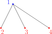
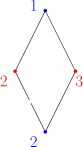
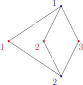
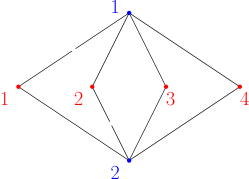
Figure 1: The space $\displaystyle\mathcal{X}$ in the cases $\displaystyle(M_{1},M_{2},M_{3})\in\{(1,3,0),(2,2,1),(2,3,2)\}$ (contractible).

Figure 2: The space $\displaystyle\mathcal{X}$ in the case $\displaystyle M_{1}=2,\,M_{2}=4,\,M_{3}=2$ (not contractible).

Proof of Theorem 3.2.

The spaces $\displaystyle\Sigma_{\rho_{i},\underline{\alpha}_{i}}$ are discrete sets of $\displaystyle M_{i}$ points, for $\displaystyle i=1,2$, that is a wedge sum of $\displaystyle M_{i}-1$ copies of $\displaystyle\mathbb{S}^{0}$. Therefore, by Theorem 3.1, $\displaystyle\Sigma_{\rho_{1},\underline{\alpha}_{1}}\star\Sigma_{\rho_{2},\underline{\alpha}_{2}}$ has the same homology as $\displaystyle\left(\mathbb{S}^{1}\right)^{\vee(M_{1}-1)(M_{2}-1)}$.
The set we have to remove from the join is made up by $\displaystyle M_{3}$ singular points $\displaystyle\{p_{m_{1}},\dots,p_{m_{M_{3}}}\}$ for some $\displaystyle\{m_{1},\dots,m_{M_{3}}\}\subset\{1,\dots,M\}$.
Defining then, for some fixed $\displaystyle\delta<\frac{1}{2}$, $\displaystyle\mathcal{Y}:=\bigcup_{j=1}^{M_{3}}B_{\delta}\left(p_{m_{j}},p_{m_{j}},\frac{1}{2}\right)$, $\displaystyle\mathcal{Y}$ retracts on $\displaystyle\left\{p_{m_{1}},\dots,p_{m_{M_{3}}}\right\}$. On the other hand, $\displaystyle\mathcal{X}\cap\mathcal{Y}$ is a disjoint union of $\displaystyle M_{3}$ punctured intervals, that is a discrete set of $\displaystyle 2M_{3}$ points, and $\displaystyle\mathcal{X}\cup\mathcal{Y}$ is the whole join. Therefore, the Mayer-Vietoris sequence yields

$$\underbrace{H_{1}(\mathcal{X}\cap\mathcal{Y})}_{0}\to H_{1}(\mathcal{X})\oplus\underbrace{H_{1}(\mathcal{Y})}_{0}\to\underbrace{H_{1}(\mathcal{X}\cup\mathcal{Y})}_{\mathbb{Z}^{(M_{1}-1)(M_{2}-1)}}\to\underbrace{\widetilde{H}_{0}(\mathcal{X}\cap\mathcal{Y})}_{\mathbb{Z}^{2M_{3}-1}}\to\widetilde{H}_{0}(\mathcal{X})\oplus\underbrace{\widetilde{H}_{0}(\mathcal{Y})}_{\mathbb{Z}^{M_{3}-1}}\to\underbrace{\widetilde{H}_{0}(\mathcal{X}\cup\mathcal{Y})}_{0}.$$

The exactness of the sequence implies that $\displaystyle b_{1}(\mathcal{X})-\widetilde{b}_{0}(\mathcal{X})=(M_{1}-1)(M_{2}-1)-M_{3}$, so if the latter number is not zero we get at least a non-trivial homology group.
Algebraic computations show that, under the assumption $\displaystyle M_{1},M_{2}\geq M_{3}$, $\displaystyle(M_{1}-1)(M_{2}-1)\neq M_{3}$ is equivalent to (24), therefore the proof is complete. ∎

4 Construction of test functions

We will now introduce some test functions from the space $\displaystyle\mathcal{X}$, introduced in Section 3, to arbitrarily low sub-levels. Such test functions will have a profile which resembles the entire solutions of the Liouville equation and of the Toda system: it will not always suffice to consider the standard bubbles

$$\varphi^{\lambda}_{p,\alpha}=-2\log\max\left\{1,(\lambda d(\cdot,p))^{2(1+\alpha)}\right\},$$

which roughly resemble the solutions of the scalar Liouville equation. This is because, when the two components are centered at the same points, a higher amount of energy is needed due to the expression of $\displaystyle Q$ (see the Introduction) which penalizes parallel gradients. . This is basically the reason that the join is punctured in (23).
We will need two more profiles for the construction of $\displaystyle\Phi^{\lambda}$, which have been considered in [23] for the regular Toda system.

$${\varphi^{\prime}}^{\lambda}_{p,\alpha_{1},\alpha_{2}}=-2\log\max\left\{1,(\lambda d(\cdot,p))^{2(2+\alpha_{1}+\alpha_{2})}\right\},$$

$${\varphi^{\prime\prime}}^{\lambda}_{p,\alpha_{1},\alpha_{2}}=-2\log\max\left\{1,\lambda^{2(2+\alpha_{1}+\alpha_{2})}d(\cdot,p)^{2(1+\alpha_{1})}\right\}.$$

We will use suitable interpolation between each of the above three profiles depending on whether the points $\displaystyle x_{i}\in\Sigma_{\rho_{i},\underline{\alpha}_{i}}$ coincide or not and depending on which of the parameters $\displaystyle\rho_{i}$ is greater or less than $\displaystyle 4\pi\left(\omega_{\underline{\alpha}_{1}}(\{x_{i}\})+\omega_{\underline{\alpha}_{2}}(\{x_{i}\})\right)$, see (8). The map $\displaystyle\Phi^{\lambda}$ will therefore be defined case by case, hence its definition will be quite lengthy and will be postponed in the proof of the theorem, rather than in its statement.
As a final remark, we considered a truncated version of the bubbles instead of the usual smooth ones. Under this change we get very similar estimates, though with simpler calculations, since truncated functions are easy to handle.

Theorem 4.1.

There exists a family of maps $\displaystyle\left\{\Phi^{\lambda}\right\}_{\lambda>2}:\mathcal{X}\to H^{1}(\Sigma)^{2}$ such that

$$J_{\rho}\left(\Phi^{\lambda}(\zeta)\right)\underset{\lambda\to+\infty}{\longrightarrow}-\infty\quad\quad\quad\text{uniformly for }\zeta\in\mathcal{X}.$$

Proof.

Let us start by defining $\displaystyle\Phi^{\lambda}(\zeta)=\left(\varphi_{1}-\frac{\varphi_{2}}{2},\varphi_{2}-\frac{\varphi_{1}}{2}\right)$ when $\displaystyle\zeta=(p_{m},p_{m},t)$ for some $\displaystyle m$. $\displaystyle\Phi^{\lambda}$ will be defined in different ways, depending on the relative positions of $\displaystyle\rho_{1},\rho_{2},\alpha_{1m},\alpha_{2m}$ in $\displaystyle\mathbb{R}$.

• $\displaystyle\rho_{1},\rho_{2}<4\pi(2+\alpha_{1m}+\alpha_{2m})$:

  $$\begin{array}[]{l}\varphi_{1}:=\left\{\begin{array}[]{ll}-2\log\max\left\{1,(\lambda d(\cdot,p_{m}))^{2(1+\alpha_{1m})}\right\}&\text{if }t<\frac{1}{2}\\ 0&\text{if }t>\frac{1}{2}\end{array}\right.\\ \varphi_{2}:=\left\{\begin{array}[]{ll}0&\text{if }t<\frac{1}{2}\\ -2\log\max\left\{1,(\lambda d(\cdot,p_{m}))^{2(1+\alpha_{2m})}\right\}&\text{if }t>\frac{1}{2}.\end{array}\right.\end{array}$$

• $\displaystyle\rho_{1}<4\pi(2+\alpha_{1m}+\alpha_{2m})<\rho_{2}$:

  $$\begin{array}[]{l}\varphi_{1}:=-2\log\max\left\{1,\max\left\{1,(\lambda t)^{2(1+\alpha_{2m})}\right\}(\lambda d(\cdot,p_{m}))^{2(1+\alpha_{1m})}\right\}\\ \varphi_{2}:=-2\log\max\left\{1,(\lambda td(\cdot,p_{m}))^{2(2+\alpha_{1m}+\alpha_{2m})}\right\}.\end{array}$$

• $\displaystyle\rho_{2}<4\pi(2+\alpha_{1m}+\alpha_{2m})<\rho_{1}$:

  $$\begin{array}[]{l}\varphi_{1}:=-2\log\max\left\{1,(\lambda(1-t)d(\cdot,p_{m}))^{2(2+\alpha_{1m}+\alpha_{2m})}\right\}\\ \varphi_{2}:=-2\log\max\left\{1,\max\left\{1,(\lambda(1-t))^{2(1+\alpha_{1m})}\right\}(\lambda d(\cdot,p_{m}))^{2(1+\alpha_{2m})}\right\}.\end{array}$$

• $\displaystyle\rho_{1},\rho_{2}>4\pi(2+\alpha_{1m}+\alpha_{2m})$:

  $$\begin{array}[]{l}\varphi_{1}:=-2\log\max\left\{1,\left(\lambda\frac{\max\{1,\lambda t\}}{\max\{1,\lambda(1-t)\}}\right)^{2+\alpha_{1m}+\alpha_{2m}}d(\cdot,p_{m})^{2(1+\alpha_{1m})},(\lambda d(\cdot,p_{m}))^{2(2+\alpha_{1m}+\alpha_{2m})}\right\}\\ \varphi_{2}:=-2\log\max\left\{1,\left(\lambda\frac{\max\{1,\lambda(1-t)\}}{\max\{1,\lambda t\}}\right)^{2+\alpha_{1m}+\alpha_{2m}}d(\cdot,p_{m})^{2(1+\alpha_{2m})},(\lambda d(\cdot,p_{m}))^{2(2+\alpha_{1m}+\alpha_{2m})}\right\}.\end{array}$$

We will need some estimates on $\displaystyle\Phi^{\lambda}$, which will be proved in three separates lemmas and which, combined, will give the proof of the theorem.∎

Convention: When using normal coordinates near the peaks of the test functions, the metric coefficients will slightly deviate from the Euclidean ones. We will then have coefficients of order $\displaystyle(1+o_{\lambda}(1))$ in front of the logarithmic terms appearing below. To keep the formulas shorter, we will omit them, as they will be harmless for the final estimates.

Lemma 4.2.

Let $\displaystyle\varphi_{1},\varphi_{2}$ be as in Theorem 4.1. Then, setting $\displaystyle\mathcal{Q}:=\int_{\Sigma}Q\left(\varphi_{1}-\frac{\varphi_{2}}{2},\varphi_{2}-\frac{\varphi_{1}}{2}\right)\mathrm{d}V_{g}$, in each case we have for $\displaystyle\lambda$ large

• $\displaystyle\mathcal{Q}=\left\{\begin{array}[]{ll}8\pi(1+\alpha_{1m})^{2}\log\lambda+O(1)&\text{if }t<\frac{1}{2}\\ 8\pi(1+\alpha_{2m})^{2}\log\lambda+O(1)&\text{if }t>\frac{1}{2}\end{array}\right.$.

• $\displaystyle\mathcal{Q}=8\pi(2+\alpha_{1m}+\alpha_{2m})^{2}\log\max\{1,\lambda t\}+8\pi(1+\alpha_{1m})^{2}\log\min\left\{\lambda,\frac{1}{t}\right\}+O(1)$.

• $\displaystyle\mathcal{Q}=8\pi(2+\alpha_{1m}+\alpha_{2m})^{2}\log\max\{1,\lambda(1-t)\}+8\pi(1+\alpha_{2m})^{2}\log\min\left\{\lambda,\frac{1}{1-t}\right\}+O(1)$.

• $\displaystyle\mathcal{Q}=8\pi(2+\alpha_{1m}+\alpha_{2m})^{2}\log\lambda+O(1)$.

Proof.

Let us start by the case $\displaystyle(<<)$. We assume $\displaystyle t<\frac{1}{2}$, since the case $\displaystyle t>\frac{1}{2}$ can be treated in the very same way just switching the indices. There holds

$$\nabla\varphi_{1}=\left\{\begin{array}[]{ll}0&\text{if }d(\cdot,p_{m})<\frac{1}{\lambda}\\ -4(1+\alpha_{1m})\frac{\nabla d(\cdot,p_{m})}{d(\cdot,p_{m})}&\text{if }d(x,p_{m})>\frac{1}{\lambda}\end{array}\right.\quad\quad\quad\nabla\varphi_{2}\equiv 0.$$

Therefore, since $\displaystyle|\nabla d(\cdot,p_{m})|=1$ a.e. on $\displaystyle\Sigma$, we get

$$\mathcal{Q}=\frac{1}{4}\int_{\Sigma}|\nabla\varphi_{1}|^{2}\mathrm{d}V_{g}=4(1+\alpha_{1m})^{2}\int_{\Sigma\setminus B_{\frac{1}{\lambda}}(p_{m})}\frac{\mathrm{d}V_{g}}{d(\cdot,p_{m})^{2}}=8\pi(1+\alpha_{1m})^{2}\log\lambda+O(1).$$ (25)

In the case $\displaystyle(<>)$ we can assume $\displaystyle\lambda t\geq 1$, since otherwise $\displaystyle\varphi_{1},\varphi_{2}$ are defined just like the previous section. We have

$$\nabla\varphi_{1}=\left\{\begin{array}[]{ll}0&\text{if }d(\cdot,p_{m})<\frac{1}{\lambda(\lambda t)^{\frac{1+\alpha_{2m}}{1+\alpha_{1m}}}}\\ -4(1+\alpha_{1m})\frac{\nabla d(\cdot,p_{m})}{d(\cdot,p_{m})}&\text{if }d(x,p_{m})>\frac{1}{\lambda(\lambda t)^{\frac{1+\alpha_{2m}}{1+\alpha_{1m}}}}\end{array}\right.,$$

$$\nabla\varphi_{2}=\left\{\begin{array}[]{ll}0&\text{if }d(\cdot,p_{m})<\frac{1}{\lambda t}\\ -4(2+\alpha_{1m}+\alpha_{2m})\frac{\nabla d(\cdot,p_{m})}{d(\cdot,p_{m})}&\text{if }d(x,p_{m})>\frac{1}{\lambda t}\end{array}\right.$$

therefore

$$\displaystyle\mathcal{Q} \displaystyle= \displaystyle\frac{1}{4}\int_{\Sigma}|\nabla\varphi_{1}|^{2}\mathrm{d}V_{g}-\frac{1}{4}\int_{\Sigma}\nabla\varphi_{1}\cdot\nabla\varphi_{2}\mathrm{d}V_{g}+\frac{1}{4}\int_{\Sigma}|\nabla\varphi_{2}|^{2}\mathrm{d}V_{g}$$

$$\displaystyle= \displaystyle 4(1+\alpha_{1m})^{2}\int_{\Sigma\setminus B_{\frac{1}{\lambda(\lambda t)^{\frac{1+\alpha_{2m}}{1+\alpha_{1m}}}}}(p_{m})}\frac{\mathrm{d}V_{g}}{d(\cdot,p_{m})^{2}}-4(2+\alpha_{1m}+\alpha_{2m})(1+\alpha_{1m})\int_{\Sigma\setminus B_{\frac{1}{\lambda t}}(p_{m})}\frac{\mathrm{d}V_{g}}{d(\cdot,p_{m})^{2}}$$

$$\displaystyle+ \displaystyle 4(2+\alpha_{1m}+\alpha_{2m})^{2}\int_{\Sigma\setminus B_{\frac{1}{\lambda t}}(p_{m})}\frac{\mathrm{d}V_{g}}{d(\cdot,p_{m})^{2}}$$

$$\displaystyle= \displaystyle 8\pi(1+\alpha_{1m})^{2}\log\lambda+8\pi(1+\alpha_{1m})(1+\alpha_{2m})\log(\lambda t)$$

$$\displaystyle- \displaystyle 8\pi(2+\alpha_{1m}+\alpha_{2m})(1+\alpha_{1m})\log(\lambda t)+8\pi(2+\alpha_{1m}+\alpha_{2m})^{2}\log(\lambda t)+O(1)$$

$$\displaystyle= \displaystyle 8\pi(2+\alpha_{1m}+\alpha_{2m})^{2}\log(\lambda t)+4\pi(1+\alpha_{2m})^{2}\log\frac{1}{t}+O(1).$$

In the case $\displaystyle(><)$ we can argue as in $\displaystyle(<>)$ just switching the indices; similar calculations also yield the last case $\displaystyle(>>)$. ∎

Lemma 4.3.

Let $\displaystyle\varphi_{1},\varphi_{2}$ be as above. Then, in each case we have:

• $$\int_{\Sigma}\varphi_{1}\mathrm{d}V_{g}=\left\{\begin{array}[]{ll}-4(1+\alpha_{1m})\log\lambda+O(1)&\text{if }t<\frac{1}{2}\\ 0&\text{if }t>\frac{1}{2}\end{array}\right.,\quad\int_{\Sigma}\varphi_{2}\mathrm{d}V_{g}=\left\{\begin{array}[]{ll}0&\text{if }t<\frac{1}{2}\\ -4(1+\alpha_{2m})\log\lambda+O(1)&\text{if }t>\frac{1}{2}.\end{array}\right.$$

• $$\int_{\Sigma}\varphi_{1}\mathrm{d}V_{g}=-4(1+\alpha_{1m})\log\lambda-4(1+\alpha_{2m})\log\max\{1,\lambda t\}+O(1),$$

  $$\int_{\Sigma}\varphi_{2}\mathrm{d}V_{g}=-4(2+\alpha_{1m}+\alpha_{2m})\log\max\{1,\lambda t\}+O(1).$$

• $$\int_{\Sigma}\varphi_{1}\mathrm{d}V_{g}=-4(2+\alpha_{1m}+\alpha_{2m})\log\max\{1,\lambda(1-t)\}+O(1),$$

  $$\int_{\Sigma}\varphi_{2}\mathrm{d}V_{g}=-4(1+\alpha_{2m})\log\lambda-4(1+\alpha_{1m})\log\max\{1,\lambda(1-t)\}+O(1).$$

• $$\int_{\Sigma}\varphi_{1}\mathrm{d}V_{g}=\int_{\Sigma}\varphi_{2}\mathrm{d}V_{g}+O(1)=-4(2+\alpha_{1m}+\alpha_{2m})\log\lambda+O(1).$$

Proof.

Let us consider the case $\displaystyle(<<),\,t<\frac{1}{2}$. Since we have

$$-4(1+\alpha_{1m})\log\max\{1,d(\cdot,p_{m})\}\leq\varphi_{1}+4(1+\alpha_{1m})\log\lambda\leq-4(1+\alpha_{1m})\log d(\cdot,p_{m}),$$

with both the first and the last function having finite average over $\displaystyle\Sigma$, we are done.

The same argument also works in all the other cases. ∎

Lemma 4.4.

Let $\displaystyle\varphi_{1},\varphi_{2}$ be as above. Then, in each case we have:

• $$\log\int_{\Sigma}\widetilde{h}_{1}e^{\varphi_{1}-\frac{\varphi_{2}}{2}}\mathrm{d}V_{g}=\left\{\begin{array}[]{ll}-2(1+\alpha_{1m})\log\lambda+O(1)&\text{if }t<\frac{1}{2}\\ 2(1+\alpha_{2m})\log\lambda+O(1)&\text{if }t>\frac{1}{2}\end{array}\right.,$$

  $$\log\int_{\Sigma}\widetilde{h}_{2}e^{\varphi_{2}-\frac{\varphi_{1}}{2}}\mathrm{d}V_{g}=\left\{\begin{array}[]{ll}2(1+\alpha_{1m})\log\lambda+O(1)&\text{if }t<\frac{1}{2}\\ -2(1+\alpha_{2m})\log\lambda+O(1)&\text{if }t>\frac{1}{2}.\end{array}\right..$$

• $$\log\int_{\Sigma}\widetilde{h}_{1}e^{\varphi_{1}-\frac{\varphi_{2}}{2}}\mathrm{d}V_{g}=-2(1+\alpha_{1m})\log\lambda-2(1+\alpha_{2m})\log\max\{1,\lambda t\},$$

  $$\log\int_{\Sigma}\widetilde{h}_{2}e^{\varphi_{2}-\frac{\varphi_{1}}{2}}\mathrm{d}V_{g}=2(1+\alpha_{1m})\min\left\{\lambda,\frac{1}{t}\right\}.$$

• $$\log\int_{\Sigma}\widetilde{h}_{1}e^{\varphi_{1}-\frac{\varphi_{2}}{2}}\mathrm{d}V_{g}=2(1+\alpha_{2m})\min\left\{\lambda,\frac{1}{1-t}\right\},$$

  $$\log\int_{\Sigma}\widetilde{h}_{2}e^{\varphi_{2}-\frac{\varphi_{1}}{2}}\mathrm{d}V_{g}=-2(1+\alpha_{2m})\log\lambda-2(1+\alpha_{1m})\log\max\{1,\lambda(1-t)\}.$$

• $$\log\int_{\Sigma}\widetilde{h}_{1}e^{\varphi_{1}-\frac{\varphi_{2}}{2}}\mathrm{d}V_{g}=-(2+\alpha_{1m}+\alpha_{2m})\log\left(\lambda\frac{\max\{1,\lambda t\}}{\max\{1,\lambda(1-t)\}}\right)+O(1)$$

  $$\log\int_{\Sigma}\widetilde{h}_{2}e^{\varphi_{2}-\frac{\varphi_{1}}{2}}\mathrm{d}V_{g}=-(2+\alpha_{1m}+\alpha_{2m})\log\left(\lambda\frac{\max\{1,\lambda(1-t)\}}{\max\{1,\lambda t\}}\right)+O(1)$$

Proof.

Again, we will just consider the first case.
Given any $\displaystyle\delta>0$, if $\displaystyle d(\cdot,p_{m})\geq\delta$ one has

$$e^{\varphi_{1}-\frac{\varphi_{2}}{2}}\geq\frac{C_{\delta}}{\lambda^{4(1+\alpha_{1m})}}\quad\quad\quad e^{\varphi_{1}-\frac{\varphi_{2}}{2}}\geq C_{\delta}\lambda^{2(1+\alpha_{1m})},$$

therefore we will suffice to consider only the integral on $\displaystyle B_{\delta}(p_{m})$:

$$\displaystyle\log\int_{B_{\delta}(p_{m})}\widetilde{h}_{1}e^{\varphi_{1}-\frac{\varphi_{2}}{2}}\mathrm{d}V_{g} \displaystyle= \displaystyle\log\int_{B_{\delta}(p_{m})}d(\cdot,p_{m})^{2\alpha_{1m}}e^{\varphi_{1}-\frac{\varphi_{2}}{2}}\mathrm{d}V_{g}+O(1)$$

$$\displaystyle= \displaystyle\log\left(\underbrace{\int_{B_{\frac{1}{\lambda}}(p_{m})}d(\cdot,p_{m})^{2\alpha_{1m}}\mathrm{d}V_{g}}_{\sim\lambda^{-2(1+\alpha_{1m})}}+\lambda^{-4(1+\alpha_{1m})}\underbrace{\int_{A_{\frac{1}{\lambda},\delta}(p_{m})}\frac{\mathrm{d}V_{g}}{d(\cdot,p_{m})^{2(2+\alpha_{1m})}}}_{\sim\lambda^{2(1+\alpha_{1m})}}\right)+O(1)$$

$$\displaystyle= \displaystyle-2(1+\alpha_{1m})\log\lambda+O(1),$$

$$\displaystyle\log\int_{B_{\delta}(p_{m})}\widetilde{h}_{1}e^{\varphi_{2}-\frac{\varphi_{1}}{2}}\mathrm{d}V_{g} \displaystyle= \displaystyle\log\left(\underbrace{\int_{B_{\frac{1}{\lambda}}(p_{m})}d(\cdot,p_{m})^{2\alpha_{2m}}\mathrm{d}V_{g}}_{\sim\lambda^{-2(1+\alpha_{2m})}}+\lambda^{2(1+\alpha_{1m})}\underbrace{\int_{A_{\frac{1}{\lambda},\delta}(p_{m})}d(\cdot,p_{m})^{2(1+\alpha_{1m}+\alpha_{2m})}\mathrm{d}V_{g}}_{\sim 1}\right)+O(1)$$

$$\displaystyle= \displaystyle 2(1+\alpha_{1m})\log\lambda+O(1),$$

∎

Proof of Theorem 4.1, continued.

From the previous lemmas we can easily prove the theorem in the case $\displaystyle x_{1}=x_{2}$. In fact, writing

$$J_{\rho}\left(\varphi_{1}-\frac{\varphi_{2}}{2},\varphi_{2}-\frac{\varphi_{1}}{2}\right)=\int_{\Sigma}Q\left(\varphi_{1}-\frac{\varphi_{2}}{2},\varphi_{2}-\frac{\varphi_{1}}{2}\right)\mathrm{d}V_{g}-\sum_{i=1}^{2}\rho_{i}\left(\log\int_{\Sigma}\widetilde{h}_{i}e^{\varphi_{i}-\frac{\varphi_{3-i}}{2}}\mathrm{d}V_{g}-\int_{\Sigma}\varphi_{i}\mathrm{d}V_{g}+\frac{1}{2}\int_{\Sigma}\varphi_{3-i}\mathrm{d}V_{g}\right),$$

we get, in each case,

• $$J_{\rho}\left(\varphi_{1}-\frac{\varphi_{2}}{2},\varphi_{2}-\frac{\varphi_{1}}{2}\right)=\left\{\begin{array}[]{ll}2(1+\alpha_{1m})(4\pi(2+\alpha_{1m})-\rho_{1})\log\lambda+O(1)&\text{if }t<\frac{1}{2}\\ 2(1+\alpha_{2m})(4\pi(2+\alpha_{2m})-\rho_{2})\log\lambda+O(1)&\text{if }t>\frac{1}{2}\end{array}\right.,$$

• $$\displaystyle J_{\rho}\left(\varphi_{1}-\frac{\varphi_{2}}{2},\varphi_{2}-\frac{\varphi_{1}}{2}\right) \displaystyle= \displaystyle 2(1+\alpha_{1m})(4\pi(1+\alpha_{1m})-\rho_{1})\log\min\left\{\lambda,\frac{1}{t}\right\}$$

  $$\displaystyle+ \displaystyle 2(2+\alpha_{1m}+\alpha_{2m})(4\pi(2+\alpha_{1m}+\alpha_{2m})-\rho_{2})\log\max\{1,\lambda t\}+O(1),$$

• $$\displaystyle J_{\rho}\left(\varphi_{1}-\frac{\varphi_{2}}{2},\varphi_{2}-\frac{\varphi_{1}}{2}\right) \displaystyle= \displaystyle 2(2+\alpha_{1m}+\alpha_{2m})(4\pi(2+\alpha_{1m}+\alpha_{2m})-\rho_{1})\log\max\{1,\lambda(1-t)\}$$

  $$\displaystyle+ \displaystyle 2(1+\alpha_{2m})(4\pi(1+\alpha_{2m})-\rho_{2})\log\min\left\{\lambda,\frac{1}{1-t}\right\}+O(1),$$

• $$\displaystyle J_{\rho}\left(\varphi_{1}-\frac{\varphi_{2}}{2},\varphi_{2}-\frac{\varphi_{1}}{2}\right) \displaystyle= \displaystyle(2+\alpha_{1m}+\alpha_{2m})(4\pi(2+\alpha_{1m}+\alpha_{2m})-\rho_{1})\log\left(\lambda\frac{\max\{1,\lambda(1-t)\}}{\max\{1,\lambda t\}}\right)$$

  $$\displaystyle+ \displaystyle(2+\alpha_{1m}+\alpha_{2m})(4\pi(2+\alpha_{1m}+\alpha_{2m})-\rho_{2})\log\left(\lambda\frac{\max\{1,\lambda t\}}{\max\{1,\lambda(1-t)\}}\right)+O(1),$$

which all tend to $\displaystyle-\infty$ independently of $\displaystyle t$.

Let us now consider the case $\displaystyle x_{1}\neq x_{2}$.
Here, we define $\displaystyle\Phi^{\lambda}$ just by interpolating linearly between the test functions defined before:

$$\Phi^{\lambda}(x_{1},x_{2},t)=\Phi^{\lambda(1-t)}(x_{1},x_{1},0)+\Phi^{\lambda t}(x_{2},x_{2},1).$$

Since $\displaystyle d(p_{m},p_{m^{\prime}})\geq\delta>0$, then the bubbles centered at $\displaystyle p_{m}$ and $\displaystyle p_{m^{\prime}}$ do not interact, therefore the estimates from Lemmas 4.2, 4.3, 4.4 also work for such test functions. We will show this fact in detail in the case $\displaystyle\rho_{1},\rho_{2}<4\pi(2+\alpha_{1m}+\alpha_{2m}),4\pi(2+\alpha_{1m^{\prime}}+\alpha_{2m^{\prime}})$. Writing

$$(\varphi_{1},\varphi_{2})=\left(-2\log\max\left\{1,(\lambda(1-t)d(\cdot,p_{m}))^{2(1+\alpha_{1m})}\right\},-2\log\max\left\{1,(\lambda td(\cdot,p_{m^{\prime}}))^{2(1+\alpha_{2m^{\prime}})}\right\}\right),$$

by the previous explicit computation of $\displaystyle\nabla\varphi_{1},\nabla\varphi_{2}$ we get

$$\displaystyle\mathcal{Q} \displaystyle= \displaystyle\frac{1}{4}\int_{B_{\delta}(p_{m})}|\nabla\varphi_{1}|^{2}\mathrm{d}V_{g}+\frac{1}{4}\int_{B_{\delta}(p_{m^{\prime}})}|\nabla\varphi_{2}|^{2}\mathrm{d}V_{g}+O(1)$$ (26)

$$\displaystyle= \displaystyle 8\pi(1+\alpha_{1m})^{2}\log\max\{1,\lambda(1-t)\}+8\pi(2+\alpha_{2m^{\prime}})^{2}\log\max\{1,\lambda t\}+O(1).$$

Moreover, by linearity,

$$\int_{\Sigma}\varphi_{1}\mathrm{d}V_{g}=-4(1+\alpha_{1m})\log\max\{1,\lambda(1-t)\}+O(1)\quad\int_{\Sigma}\varphi_{2}\mathrm{d}V_{g}=-4(1+\alpha_{2m^{\prime}})\log\max\{1,\lambda t\}+O(1).$$ (27)

Finally, as before the integral of $\displaystyle\widetilde{h}_{1}e^{\varphi_{1}-\frac{\varphi_{2}}{2}}$ is negligible outside $\displaystyle B_{\delta}(p_{m})$, and inside the ball we have $\displaystyle\frac{1}{C_{\delta}}\leq\left|\varphi_{2}-\int_{\Sigma}\varphi_{2}\mathrm{d}V_{g}\right|\leq C$ on $\displaystyle B_{\delta}(p_{m})$, hence

$$\displaystyle\log\int_{\Sigma}\widetilde{h}_{1}e^{\varphi_{1}-\frac{\varphi_{2}}{2}}\mathrm{d}V_{g} \displaystyle= \displaystyle\log\left(\max\{1,\lambda t\}^{2(1+\alpha_{2m^{\prime}})}\int_{B_{\frac{1}{\max\{1,\lambda(1-t)\}}}(p_{m})}d(\cdot,p_{m})^{2\alpha_{1m}}\mathrm{d}V_{g}\right.$$ (28)

$$\displaystyle+ \displaystyle\left.\max\{1,\lambda t\}^{2(1+\alpha_{2m^{\prime}})}\max\{1,\lambda(1-t)\}^{2(1+\alpha_{1m})}\int_{A_{\frac{1}{\lambda},\delta}(p_{m})}\frac{\mathrm{d}V_{g}}{d(\cdot,p_{m})^{2(2+\alpha_{1m})}}\right)+O(1)$$

$$\displaystyle= \displaystyle 2(1+\alpha_{2m^{\prime}})\log\max\{1,\lambda t\}-2(1+\alpha_{1m})\log\max\{1,\lambda(1-t)\}+O(1)$$

and similarly

$$\log\int_{\Sigma}\widetilde{h}_{2}e^{\varphi_{2}-\frac{\varphi_{1}}{2}}\mathrm{d}V_{g}=2(1+\alpha_{1m})\log\max\{1,\lambda(1-t)\}-2(1+\alpha_{1m^{\prime}})\log\max\{1,\lambda t\}+O(1).$$

Therefore, by (26), (27) and (28) we deduce

$$\displaystyle J_{\rho}\left(\varphi_{1}-\frac{\varphi_{2}}{2},\varphi_{2}-\frac{\varphi_{1}}{2}\right) \displaystyle= \displaystyle 2(1+\alpha_{1m})(4\pi(1+\alpha_{1m})-\rho_{1})\log\max\{1,\lambda(1-t)\}$$

$$\displaystyle+ \displaystyle 2(1+\alpha_{2m^{\prime}})(4\pi(1+\alpha_{2m^{\prime}})-\rho_{2})\log\max\{1,\lambda t\}+O(1).$$

This concludes the proof. ∎

5 Improved Moser-Trudinger inequalities

In this section we will deduce some improved Moser-Trudinger inequalities when the two components have the same center and mass of concentration, in the sense defined by Lemma 2.11.

Theorem 5.1.

Let $\displaystyle\beta_{i}(u),\varsigma_{i}(u)$ be as in Corollary 2.12. There exists $\displaystyle L\gg 0$ such that if

$$\left\{\begin{array}[]{ll}\beta_{1}(u)=\beta_{2}(u)=p_{m}&\text{with }\rho_{1},\rho_{2}<4\pi(2+\alpha_{1m}+\alpha_{2m})\\ \varsigma_{1}(u)=\varsigma_{2}(u)&\end{array}\right.,$$

then $\displaystyle J_{\rho}(u)\geq-L$.

Theorem 5.1 is based on the following two lemmas, inspired by [34]. Basically, we assume $\displaystyle u_{1}$ and $\displaystyle u_{2}$ to have the same center and scale of concentration and we provide local estimates in a ball which is roughly centered at the center of mass and whose radius is roughly the same as the scale of concentration. Inner estimates use a dilation argument, outer estimates use a Kelvin transform. With respect to the above-cited paper, we also have to consider concentration around the boundary of the ball, hence we will combine those arguments with Theorem 2.8 and Lemma 2.9.

Lemma 5.2.

For any $\displaystyle\varepsilon>0,\,\alpha_{1},\alpha_{2}\in(-1,0]$ there exists $\displaystyle C=C_{\varepsilon}$ such that for any $\displaystyle p\in\Sigma,\,s>0$ small enough and $\displaystyle u\in H^{1}(\Sigma)^{2}$ one has

$$\displaystyle 4\pi\sum_{i=1}^{2}(1+\alpha_{i})\left(\log\int_{B_{\frac{s}{2}}(p)}d(\cdot,p)^{2\alpha_{i}}e^{u_{i}}\mathrm{d}V_{g}-\fint_{B_{s}(p)}u_{i}\mathrm{d}V_{g}\right)-8\pi\left((1+\alpha_{1})^{2}+(1+\alpha_{2})^{2}\right)\log s$$

$$\displaystyle\leq \displaystyle(1+\varepsilon)\int_{B_{s}(p)}Q(u)\mathrm{d}V_{g}+C,$$

$$\displaystyle 4\pi(1+\alpha_{1})\left(\log\int_{B_{\frac{s}{8}}(p)}d(\cdot,p)^{2\alpha_{1}}e^{u_{1}}\mathrm{d}V_{g}-\fint_{B_{s}(p)}u_{1}\mathrm{d}V_{g}\right)$$

$$\displaystyle+ \displaystyle 2\pi\min\{1,2+\alpha_{1}+\alpha_{2}\}\left(\log\int_{A_{\frac{s}{4},s}(p)}d(\cdot,p)^{2\alpha_{2}}e^{u_{2}}\mathrm{d}V_{g}-\fint_{B_{s}(p)}u_{2}\mathrm{d}V_{g}\right)$$

$$\displaystyle- \displaystyle 4\pi\left(2(1+\alpha_{1})^{2}+\min\{1,2+\alpha_{1}+\alpha_{2}\}(1+\alpha_{2})\right)\log s$$

$$\displaystyle\leq \displaystyle(1+\varepsilon)\int_{B_{s}(p)}Q(u)\mathrm{d}V_{g}+C,$$

$$\displaystyle 2\pi\sum_{i=1}^{2}\min\{1,2+\alpha_{1}+\alpha_{2}\}\left(\log\int_{A_{\frac{s}{2},s}(p)}d(\cdot,p)^{2\alpha_{i}}e^{u_{i}}\mathrm{d}V_{g}-\fint_{B_{s}(p)}u_{i}\mathrm{d}V_{g}\right)$$

$$\displaystyle- \displaystyle 4\pi\min\left\{2+\alpha_{1}+\alpha_{2},(2+\alpha_{1}+\alpha_{2})^{2}\right\}\log s$$

$$\displaystyle\leq \displaystyle(1+\varepsilon)\int_{B_{s}(p)}Q(u)\mathrm{d}V_{g}+C.$$ (31)

The last statement holds true if $\displaystyle B_{s}(p)$ is replaced by $\displaystyle\Omega_{s}$ simply connected belonging to $\displaystyle\mathfrak{A}_{\delta s}$ (see (16)) and such that $\displaystyle B_{\left(\frac{1}{2}+\delta\right)s}(p)\subset\Omega_{s}\subset B_{\frac{s}{\delta}}(p)$ for some $\displaystyle\delta>0$, with $\displaystyle C$ replaced with some $\displaystyle C_{\delta}>0$.

Proof.

By assuming $\displaystyle s$ small enough, we can suppose the metric to be flat on $\displaystyle B_{s}(p)$, up to negligible remainder terms. Therefore, we will assume to work on a Euclidean ball centered at the origin: we will indicate such balls simply as $\displaystyle B_{s}$, omitting their center, and we will use a similar convention for annuli. Moreover, we will write $\displaystyle|x|$ for $\displaystyle d(x,p)$.
Consider the dilation $\displaystyle v_{i}(z)=u_{i}(sz)$ for $\displaystyle z\in B_{1}$. It verifies, for $\displaystyle r\in\left\{\frac{1}{8},\frac{1}{4},\frac{1}{2}\right\}$

$$\int_{B_{r}}|z|^{2\alpha_{i}}e^{v_{i}(z)}\mathrm{d}z=s^{-2-2\alpha_{i}}\int_{B_{rs}}|x|^{2\alpha_{i}}e^{u_{i}(x)}\mathrm{d}x,$$

$$\int_{A_{r,1}}|z|^{2\alpha_{i}}e^{v_{i}(z)}\mathrm{d}z=s^{-2-2\alpha_{i}}\int_{A_{rs,s}}|x|^{2\alpha_{i}}e^{u_{i}(x)}\mathrm{d}x.$$

$$\int_{B_{1}}Q(v(z))\mathrm{d}z=\int_{B_{s}}Q(u(x))\mathrm{d}x,\quad\quad\quad\fint_{B_{1}}v(z)\mathrm{d}z=\fint_{B_{s}}u(x)\mathrm{d}x,$$

To get (5.2), it suffices to apply (17) to $\displaystyle v=(v_{1},v_{2})$:

$$\displaystyle 4\pi\sum_{i=1}^{2}(1+\alpha_{i})\left(\log\int_{B_{\frac{s}{2}}}|x|^{2\alpha_{i}}e^{u_{i}(x)}\mathrm{d}x-\fint_{B_{s}}u_{i}(x)\mathrm{d}x-2(1+\alpha_{i})\log s\right)$$

$$\displaystyle\leq \displaystyle 4\pi\sum_{i=1}^{2}(1+\alpha_{i})\left(\log\int_{B_{\frac{1}{2}}}|z|^{2\alpha_{i}}e^{v_{i}(z)}\mathrm{d}z-\fint_{B_{1}}v_{i}(z)\mathrm{d}z\right)$$

$$\displaystyle\leq \displaystyle(1+\varepsilon)\int_{B_{1}}Q(v(z))\mathrm{d}z+C$$

$$\displaystyle= \displaystyle(1+\varepsilon)\int_{B_{s}}Q(u(x))\mathrm{d}x+C.$$

For (5.2), one has to use (18) on $\displaystyle v$, and the elementary fact that $\displaystyle\frac{1}{C}\leq|z|^{2\alpha_{2}}\leq C$ on $\displaystyle A_{\frac{1}{4},1}$:

$$\displaystyle 4\pi(1+\alpha_{1})\left(\log\int_{B_{\frac{s}{8}}}|x|^{2\alpha_{1}}e^{u_{1}(x)}\mathrm{d}x-\fint_{B_{s}}u_{1}(x)\mathrm{d}x-2(1+\alpha_{1})\log s\right)$$

$$\displaystyle+ \displaystyle 2\pi\min\{1,2+\alpha_{1}+\alpha_{2}\}\left(\log\int_{A_{\frac{s}{4},s}}|x|^{2\alpha_{2}}e^{u_{2}(x)}\mathrm{d}V_{g}(x)-\fint_{B_{s}}u_{2}(x)\mathrm{d}x-2(1+\alpha_{2})\log s\right)$$

$$\displaystyle\leq \displaystyle 4\pi(1+\alpha_{1})\left(\log\int_{B_{\frac{1}{8}}}|z|^{2\alpha_{1}}e^{v_{1}(z)}\mathrm{d}z-\fint_{B_{1}}v_{1}(z)\mathrm{d}x\right)$$

$$\displaystyle+ \displaystyle 2\pi\min\{1,2+\alpha_{1}+\alpha_{2}\}\left(\log\int_{A_{\frac{1}{4},1}}e^{v_{2}(z)}\mathrm{d}V_{g}(z)-\fint_{B_{1}}v_{2}(z)\mathrm{d}z\right)+C$$

$$\displaystyle\leq \displaystyle(1+\varepsilon)\int_{B_{1}}Q(v(z))\mathrm{d}z+C$$

$$\displaystyle= \displaystyle(1+\varepsilon)\int_{B_{s}}Q(u(x))\mathrm{d}x+C.$$

Finally, (31) follows from Theorem 2.8:

$$\displaystyle 2\pi\sum_{i=1}^{2}\min\{1,2+\alpha_{1}+\alpha_{2}\}\left(\log\int_{A_{\frac{s}{2},s}}|x|^{2\alpha_{i}}e^{u_{i}(x)}\mathrm{d}x-\fint_{B_{s}}u_{i}(x)\mathrm{d}x-2(1+\alpha_{i})\log s\right)$$

$$\displaystyle\leq \displaystyle 2\pi\sum_{i=1}^{2}\min\{1,2+\alpha_{1}+\alpha_{2}\}\left(\log\int_{A_{\frac{1}{2},1}}e^{v_{i}(z)}\mathrm{d}z-\fint_{B_{1}}v_{i}(z)\mathrm{d}z\right)+C$$

$$\displaystyle\leq \displaystyle(1+\varepsilon)\int_{B_{1}}Q(v(z))\mathrm{d}z+C$$

$$\displaystyle= \displaystyle(1+\varepsilon)\int_{B_{s}}Q(u(x))\mathrm{d}x+C.$$

The final remark holds true because of the final remarks in Theorem 2.8 and Lemma 2.13. ∎

Lemma 5.3.

For any $\displaystyle\varepsilon>0,\,\alpha_{1},\alpha_{2}\in(-1,0],\,d>0$ small there exists $\displaystyle C=C_{\varepsilon}$ such that for any $\displaystyle p\in\Sigma,\,s\in\left(0,\frac{d}{8}\right)$ and $\displaystyle u\in H^{1}(\Sigma)^{2}$ with $\displaystyle u_{i}|_{\partial B_{d}(p)}\equiv 0$ one has

$$\displaystyle 4\pi\sum_{i=1}^{2}(1+\alpha_{3-i})\log\int_{A_{2s,d}(p)}d(\cdot,p)^{2\alpha_{i}}e^{u_{i}}\mathrm{d}V_{g}+4\pi(1+\varepsilon)\sum_{i=1}^{2}(1+\alpha_{i})\fint_{B_{s}(p)}u_{i}\mathrm{d}V_{g}$$ (32)

$$\displaystyle+ \displaystyle 8\pi(1+\varepsilon)\left((1+\alpha_{1})^{2}+(1+\alpha_{2})^{2}\right)\log s$$

$$\displaystyle\leq \displaystyle\int_{A_{s,d}(p)}Q(u)\mathrm{d}V_{g}+\varepsilon\int_{B_{d}(p)}Q(u)\mathrm{d}V_{g}+C,$$

$$\displaystyle 4\pi(1+\alpha_{2})\log\int_{A_{8s,d}(p)}d(\cdot,p)^{2\alpha_{1}}e^{u_{1}}\mathrm{d}V_{g}+4\pi(1+\varepsilon)(1+\alpha_{1})\fint_{B_{s}(p)}u_{1}\mathrm{d}V_{g}$$ (33)

$$\displaystyle+ \displaystyle 2\pi\min\{1,2+\alpha_{1}+\alpha_{2}\}\left(\log\int_{A_{s,4s}(p)}d(\cdot,p)^{2\alpha_{2}}e^{u_{2}}\mathrm{d}V_{g}+(1+\varepsilon)\fint_{B_{s}(p)}u_{2}\mathrm{d}V_{g}\right)$$

$$\displaystyle+ \displaystyle 4\pi(1+\varepsilon)\left(2(1+\alpha_{1})^{2}+\min\{1,2+\alpha_{1}+\alpha_{2}\}(1+\alpha_{2})\right)\log s$$

$$\displaystyle\leq \displaystyle\int_{A_{s,d}(p)}Q(u)\mathrm{d}V_{g}+\varepsilon\int_{B_{d}(p)}Q(u)\mathrm{d}V_{g}+C,$$

$$\displaystyle 2\pi\sum_{i=1}^{2}\min\{1,2+\alpha_{1}+\alpha_{2}\}\left(\log\int_{A_{s,2s}(p)}d(\cdot,p)^{2\alpha_{i}}e^{u_{i}}\mathrm{d}V_{g}+(1+\varepsilon)\fint_{B_{s}(p)}u_{i}\mathrm{d}V_{g}\right)$$

$$\displaystyle+ \displaystyle 4\pi(1+\varepsilon)\min\left\{2+\alpha_{1}+\alpha_{2},(2+\alpha_{1}+\alpha_{2})^{2}\right\}\log s$$

$$\displaystyle\leq \displaystyle\int_{A_{s,d}(p)}Q(u)\mathrm{d}V_{g}+\varepsilon\int_{B_{d}(p)}Q(u)\mathrm{d}V_{g}+C.$$

The last statement holds true if $\displaystyle B_{s}(p)$ is replaced by a simply connected domain $\displaystyle\Omega_{s}$ belonging to $\displaystyle\mathfrak{A}_{\delta s}$ and such that $\displaystyle B_{\delta s}(p)\subset\Omega_{s}\subset B_{\left(2+\frac{1}{\delta}\right)s}(p)$ for some $\displaystyle\delta>0$, with $\displaystyle C$ replaced by some $\displaystyle C_{\delta}>0$.

Proof.

Just like Lemma 5.2, we will work with flat Euclidean balls, whose centers will be omitted. Moreover, it will not be restrictive to assume $\displaystyle\fint_{B_{d}}u_{i}(x)\mathrm{d}x=0$ for both $\displaystyle i$’s.
Define, for $\displaystyle z\in B_{d}$ and $\displaystyle c_{1},c_{2}\leq-2(2+\alpha_{1}+\alpha_{2})$,

$$v_{i}(z):=\left\{\begin{array}[]{ll}(2c_{i}-c_{3-i})\log s&\text{if }z\in B_{s}\\ u_{i}\left(ds\frac{z}{|z|^{2}}\right)+(2c_{i}-c_{3-i})\log|z|&\text{if }z\in A_{s,d}\end{array}\right.$$

By a change of variable we find, for $\displaystyle r\in\left\{\frac{1}{8},\frac{1}{4},\frac{1}{2}\right\}$,

$$\displaystyle\int_{A_{s,rd}}|z|^{-4-2\alpha_{i}-2c_{i}+c_{3-i}}e^{v_{i}(z)}\mathrm{d}z=\int_{B_{s,rd}}|z|^{-4-2\alpha_{i}}e^{u_{i}\left(ds\frac{z}{|z|^{2}}\right)}\mathrm{d}z=(ds)^{-2-2\alpha_{i}}\int_{A_{\frac{s}{r},d}}|x|^{2\alpha_{i}}e^{u_{i}(x)}\mathrm{d}x$$

$$\displaystyle\int_{A_{rd,d}}e^{v_{i}(z)}\mathrm{d}z\sim\int_{A_{rd,d}}|z|^{-4-2\alpha_{i}-2c_{i}+c_{3-i}}e^{v_{i}(z)}\mathrm{d}z=(ds)^{-2-2\alpha_{i}}\int_{A_{s,\frac{s}{r}}}|x|^{2\alpha_{i}}e^{u_{i}(x)}\mathrm{d}x.$$

Moreover, by Lemma 2.13, we get

$$\displaystyle\left|\fint_{B_{s}}u_{i}(x)\mathrm{d}x-\fint_{B_{d}}v_{i}(z)\mathrm{d}z\right| \displaystyle\leq \displaystyle\left|\fint_{B_{s}}u_{i}(x)\mathrm{d}x-\fint_{\partial B_{s}}u_{i}(x)\mathrm{d}x\right|+\left|\fint_{\partial B_{s}}u_{i}(x)\mathrm{d}x-\fint_{\partial B_{d}}v_{i}(z)\mathrm{d}z\right|$$

$$\displaystyle+ \displaystyle\left|\fint_{B_{d}}v_{i}(z)\mathrm{d}z-\fint_{B_{d}}v_{i}(z)\mathrm{d}z\right|$$

$$\displaystyle\leq \displaystyle C\sqrt{\int_{B_{s}}|\nabla u(x)|^{2}\mathrm{d}x}+|(2c_{i}-c_{3-i})\log d|+C\sqrt{\int_{B_{d}}|\nabla v(z)|^{2}\mathrm{d}z}\leq$$

$$\displaystyle\leq \displaystyle\varepsilon^{\prime}\int_{B_{s}}Q(u(x))\mathrm{d}x+\varepsilon^{\prime}\int_{B_{d}}Q(v(z))\mathrm{d}z+C_{d}.$$

Concerning the Dirichlet integral, we can write

$$\displaystyle\int_{B_{d}}\nabla v_{i}(z)\cdot\nabla v_{j}(z)\mathrm{d}z \displaystyle= \displaystyle\int_{A_{s,d}}\left(\frac{d^{2}s^{2}}{|z|^{4}}\nabla u_{i}\left(sd\frac{z}{|z|^{2}}\right)\cdot\nabla u_{j}\left(ds\frac{z}{|z|^{2}}\right)-(2c_{i}-c_{3-i})sd\frac{z}{|z|^{2}}\cdot\nabla u_{j}\left(ds\frac{z}{|z|^{2}}\right)\right.$$

$$\displaystyle- \displaystyle\left.(2c_{j}-c_{3-j})sd\frac{z}{|z|^{2}}\cdot\nabla u_{i}\left(sd\frac{z}{|z|^{2}}\right)+\frac{(2c_{i}-c_{3-i})(2c_{j}-c_{3-j})}{|z|^{2}}\right)\mathrm{d}z$$

$$\displaystyle= \displaystyle\int_{A_{s,d}}\nabla u_{i}(x)\cdot\nabla u_{j}(x)\mathrm{d}x-(2c_{i}-c_{3-i})\int_{A_{s,d}}\frac{x}{|x|^{2}}\cdot\nabla u_{j}(x)\mathrm{d}x$$

$$\displaystyle- \displaystyle(2c_{j}-c_{3-j})\int_{A_{s,d}}\frac{x}{|x|^{2}}\cdot\nabla u_{i}(x)\mathrm{d}x-2\pi(2c_{i}-c_{3-i})(2c_{j}-c_{3-j})\log s$$

$$\displaystyle+ \displaystyle 2\pi(2c_{i}-c_{3-i})(2c_{j}-c_{3-j})\log d$$

$$\displaystyle= \displaystyle\int_{A_{s,d}}\nabla u_{i}(x)\cdot\nabla u_{j}(x)\mathrm{d}x+2\pi(2c_{i}-c_{3-i})\fint_{\partial B_{s}}u_{j}(x)\mathrm{d}x$$

$$\displaystyle+ \displaystyle 2\pi(2c_{j}-c_{3-j})\fint_{\partial B_{s}}u_{i}(x)\mathrm{d}x-2\pi(2c_{i}-c_{3-i})(2c_{j}-c_{3-j})\log s+C_{d},$$

therefore, since $\displaystyle v$ has constant components in $\displaystyle B_{s}$,

$$\int_{B_{d}}Q(v(z))\mathrm{d}z=\int_{A_{s,d}}Q(u(x))\mathrm{d}x+2\pi\sum_{i=1}^{2}c_{i}\fint_{\partial B_{s}}u_{i}(x)\mathrm{d}x-2\pi\left(c_{1}^{2}-c_{1}c_{2}+c_{2}^{2}\right)\log s+C.$$

The assertion of the lemma follows by applying Lemma 2.9 on $\displaystyle B_{d}$ to $\displaystyle v$ with different choices of $\displaystyle c_{1},c_{2}$. If we take $\displaystyle c_{1}=c_{2}=-2(2+\alpha_{1}+\alpha_{2})$, then we get

$$\displaystyle 4\pi\sum_{i=1}^{2}(1+\alpha_{3-i})\log\int_{A_{2s,d}}|x|^{2\alpha_{i}}e^{u_{i}(x)}\mathrm{d}x$$

$$\displaystyle\leq \displaystyle 4\pi\sum_{i=1}^{2}(1+\alpha_{3-i})\left(\log\int_{B_{\frac{d}{2}}}|z|^{2\alpha_{3-i}}e^{v_{i}(z)}\mathrm{d}z+2(1+\alpha_{i})\log s\right)+C$$

$$\displaystyle\leq \displaystyle(1+\varepsilon^{\prime})\int_{B_{d}}Q(v(z))\mathrm{d}z+4\pi\sum_{i=1}^{2}(1+\alpha_{3-i})\fint_{B_{d}}v_{i}(z)\mathrm{d}z+16\pi(1+\alpha_{1})(1+\alpha_{2})\log s+C$$

$$\displaystyle\leq \displaystyle(1+\varepsilon^{\prime\prime})\int_{A_{s,d}}Q(u(x))\mathrm{d}x+\varepsilon^{\prime\prime}\int_{B_{d}}Q(u(x))\mathrm{d}x+4\pi\sum_{i=1}^{2}(1+\alpha_{3-i})\fint_{B_{s}}u_{i}(x)\mathrm{d}x$$

$$\displaystyle- \displaystyle 4\pi(1+\varepsilon^{\prime\prime})(2+\alpha_{1}+\alpha_{2})\sum_{i=2}^{2}\fint_{\partial B_{s}}u_{i}(x)\mathrm{d}x+8\pi\left(2(1+\alpha_{1})(1+\alpha_{2})-(1+\varepsilon^{\prime\prime})(2+\alpha_{1}+\alpha_{2})^{2}\right)\log s+C$$

$$\displaystyle\leq \displaystyle(1+\varepsilon^{\prime\prime\prime})\int_{B_{s}}Q(u(x))\mathrm{d}x+\varepsilon^{\prime\prime\prime}\int_{B_{d}}Q(u(x))\mathrm{d}x+4\pi\sum_{i=1}^{2}((1+\alpha_{3-i})-(1+\varepsilon^{\prime\prime\prime})(2+\alpha_{1}+\alpha_{2}))\fint_{B_{s}}u_{i}(x)\mathrm{d}x$$

$$\displaystyle+ \displaystyle 8\pi\left(2(1+\alpha_{1})(1+\alpha_{2})-(1+\varepsilon^{\prime\prime\prime})(2+\alpha_{1}+\alpha_{2})^{2}\right)\log s+C,$$

that is, re-naming $\displaystyle\varepsilon$ properly, (32).

Choosing $\displaystyle c_{1}=-2(2+\alpha_{1}+\alpha_{2})$ and $\displaystyle c_{2}=-2\min\{1,2+\alpha_{1}+\alpha_{2}\}=:-2m$, we get

$$\displaystyle 4\pi(1+\alpha_{2})\log\int_{A_{8s,d}}|x|^{2\alpha_{1}}e^{u_{1}(x)}\mathrm{d}x+2\pi m\log\int_{A_{s,4s}}|x|^{2\alpha_{2}}e^{u_{2}(x)}\mathrm{d}x$$

$$\displaystyle\leq \displaystyle 4\pi(1+\alpha_{2})\log\int_{B_{\frac{d}{8}}}|z|^{\max\{2+2\alpha_{1}+4\alpha_{2},2\alpha_{2}\}}e^{v_{1}(z)}\mathrm{d}z+2\pi m\log\int_{A_{\frac{d}{4},d}}e^{v_{2}(z)}\mathrm{d}z$$

$$\displaystyle+ \displaystyle 4\pi(2(1+\alpha_{1})(1+\alpha_{2})+m(1+\alpha_{2}))\log s+C$$

$$\displaystyle\leq \displaystyle(1+\varepsilon^{\prime})\int_{B_{d}}Q(v(z))\mathrm{d}z+4\pi(1+\alpha_{2})\fint_{B_{d}}v_{1}(z)\mathrm{d}z+2\pi m\fint_{B_{d}}v_{2}(z)\mathrm{d}z$$

$$\displaystyle+ \displaystyle 4\pi(1+\alpha_{2})(2(1+\alpha_{1})+m)\log s+C$$

$$\displaystyle\leq \displaystyle(1+\varepsilon^{\prime\prime})\int_{A_{s,d}}Q(u(x))\mathrm{d}x+\varepsilon^{\prime\prime}\int_{B_{d}}Q(u(x))\mathrm{d}x+4\pi(1+\alpha_{2})\fint_{B_{s}}u_{1}(x)\mathrm{d}x+2\pi m\fint_{B_{s}}u_{2}(x)\mathrm{d}x$$

$$\displaystyle- \displaystyle 4\pi(1+\varepsilon^{\prime\prime})(2+\alpha_{1}+\alpha_{2})\fint_{\partial B_{s}}u_{1}(x)\mathrm{d}x-4\pi(1+\varepsilon^{\prime\prime})m\fint_{\partial B_{s}}u_{2}(x)\mathrm{d}x$$

$$\displaystyle+ \displaystyle 4\pi\left((1+\alpha_{2})(2(1+\alpha_{1})+m)-2(1+\varepsilon^{\prime\prime})\left((2+\alpha_{1}+\alpha_{2})^{2}-m(2+\alpha_{1}+\alpha_{2})+m^{2}\right)\right)\log s+C$$

$$\displaystyle\leq \displaystyle(1+\varepsilon^{\prime\prime\prime})\int_{A_{s,d}}Q(u(x))\mathrm{d}x+\varepsilon^{\prime\prime\prime}\int_{B_{d}}Q(u(x))\mathrm{d}x$$

$$\displaystyle+ \displaystyle 4\pi((1+\alpha_{2})-(1+\varepsilon^{\prime\prime\prime})(2+\alpha_{1}+\alpha_{2}))\fint_{B_{s}}u_{1}(x)\mathrm{d}x-2\pi(1+2\varepsilon^{\prime\prime\prime})m\fint_{B_{s}}u_{2}(x)\mathrm{d}x$$

$$\displaystyle+ \displaystyle 4\pi((1+\alpha_{2})(2(1+\alpha_{1})+m)-2(1+\varepsilon^{\prime\prime\prime})((1+\alpha_{1})(2+\alpha_{1}+\alpha_{2})+(1+\alpha_{2})m))\log s+C,$$

namely (33).

Finally, taking $\displaystyle c_{1}=c_{2}=-2m$ one finds (5.3):

$$\displaystyle 2\pi\sum_{i=1}^{2}\min\{1,2+\alpha_{1}+\alpha_{2}\}\log\int_{A_{s,2s}}|x|^{2\alpha_{i}}e^{u_{i}(x)}\mathrm{d}x$$

$$\displaystyle\leq \displaystyle 2\pi\sum_{i=1}^{2}m\left(\log\int_{A_{\frac{d}{2},d}}e^{v_{i}(z)}\mathrm{d}z+2(1+\alpha_{i})\log s\right)+C$$

$$\displaystyle\leq \displaystyle(1+\varepsilon^{\prime})\int_{B_{d}}Q(v(z))\mathrm{d}z+2\pi m\sum_{i=1}^{2}\fint_{B_{d}}v_{i}(z)\mathrm{d}z+4\pi m(2+\alpha_{1}+\alpha_{2})\log s+C$$

$$\displaystyle\leq \displaystyle(1+\varepsilon^{\prime\prime})\int_{B_{d}}Q(u(x))\mathrm{d}x+\varepsilon^{\prime\prime}\int_{B_{d}}Q(u(x))\mathrm{d}x+2\pi m\sum_{i=1}^{2}\fint_{B_{s}}u_{i}(x)\mathrm{d}x$$

$$\displaystyle- \displaystyle 4\pi(1+\varepsilon^{\prime\prime})m\sum_{i=1}^{2}\fint_{\partial B_{s}}u_{i}(x)\mathrm{d}x+4\pi\left(m(2+\alpha_{1}+\alpha_{2})-2(1+\varepsilon^{\prime\prime})m^{2}\right)\log s+C$$

$$\displaystyle\leq \displaystyle(1+\varepsilon^{\prime\prime})\int_{B_{d}}Q(u(x))\mathrm{d}x+\varepsilon^{\prime\prime\prime}\int_{B_{d}}Q(u(x))\mathrm{d}x-2\pi(1+2\varepsilon^{\prime\prime\prime})m\sum_{i=1}^{2}\fint_{B_{s}}u_{i}(x)\mathrm{d}x$$

$$\displaystyle- \displaystyle 4\pi(1+2\varepsilon^{\prime\prime\prime})m(2+\alpha_{1}+\alpha_{2})\log s+C.$$

The final remark holds true, like in Lemma 5.2, because of the final remarks in Theorem 2.8 and Lemma 2.13. In particular, when integrating by parts, one gets

$$\int_{B_{\delta}\setminus\Omega_{s}}\frac{x}{|x|^{2}}\cdot\nabla u_{i}(x)\mathrm{d}x=\int_{\partial\Omega_{s}}u_{i}(x)\underbrace{\frac{x}{|x|^{2}}\cdot\nu(x)}_{=:f(x)}\mathrm{d}x=,$$

with $\displaystyle\int_{\partial\Omega_{s}}f(x)\mathrm{d}x=2\pi$ and $\displaystyle|f(x)|\leq\frac{C}{s}\leq\frac{C}{|\Omega_{s}|}$, therefore, by the Poincaré-Wirtinger inequality

$$\displaystyle\left|\int_{\partial\Omega_{s}}u_{i}(x)f(x)\mathrm{d}x-2\pi\int_{\partial\Omega_{s}}u_{i}(y)\mathrm{d}y\right| \displaystyle= \displaystyle\left|\int_{\partial\Omega_{s}}f(x)\left(u_{i}(x)-\fint_{\partial\Omega_{s}}u_{i}(y)\mathrm{d}y\right)\mathrm{d}y\right|$$

$$\displaystyle\leq \displaystyle C\fint_{\partial\Omega_{s}}\left|u_{i}(x)-\fint_{\partial\Omega_{s}}u(y)\mathrm{d}y\right|\mathrm{d}x$$

$$\displaystyle\leq \displaystyle C\int_{\Omega_{s}}|\nabla u_{i}(x)|^{2}\mathrm{d}x$$

$$\displaystyle\leq \displaystyle\varepsilon\int_{\Omega_{s}}Q(u(x))\mathrm{d}x+C_{\varepsilon},$$

and $\displaystyle\left|\fint_{\partial\Omega_{s}}u_{i}(x)\mathrm{d}x-\fint_{\partial B_{s}}u_{i}(x)\mathrm{d}x\right|\leq\varepsilon\int_{\Omega_{s}}Q(u(x))\mathrm{d}x+C_{\varepsilon}$ by Lemma 2.13. ∎

To prove Theorem 5.1 we also need the following lemma. It basically allows us to divide a disk in two domains in such a way that the integrals of two given functions are both split exactly in two.

Lemma 5.4.

Consider $\displaystyle B:=B_{1}(0)\subset\mathbb{R}^{2}$ and $\displaystyle f_{1},f_{2}\in L^{1}(B)$ such that $\displaystyle f_{i}>0$ a.e. $\displaystyle x\in B$ for both $\displaystyle i=1,2$ and $\displaystyle\int_{B}f_{1}(x)\mathrm{d}x=\int_{B}f_{2}(x)\mathrm{d}x=1$. Then, there exist $\displaystyle\theta\in\mathbb{S}^{1}$ and $\displaystyle a\in(-1,1)$ such that

$$\int_{\{x\in B:\,x\cdot\theta<a\}}f_{1}(x)\mathrm{d}x=\int_{\{x\in B:\,x\cdot\theta>a\}}f_{2}(x)\mathrm{d}x=\frac{1}{2}$$

Proof.

Define, for $\displaystyle(\theta,a)\in\mathbb{S}^{1}\times(-1,1)$,

$$I_{1}(\theta,a):=\int_{\{x\in B:\,x\cdot\theta<a_{1}(\theta)\}}f_{1}(x)\mathrm{d}x.$$

For any given $\displaystyle\theta$ there exists a unique $\displaystyle a_{1}(\theta)$, smoothly depending on $\displaystyle\theta$ such that $\displaystyle I_{1}(\theta,a_{1}(\theta))=\frac{1}{2}$. Define similarly $\displaystyle I_{2}(\theta,a)$ and $\displaystyle a_{2}(\theta)$.
Let us now show the existence of $\displaystyle\theta$ such that $\displaystyle a_{1}(\theta)=a_{2}(\theta):=a$, hence the proof of the lemma will follow. Suppose by contradiction that $\displaystyle a_{1}(\theta)<a_{2}(\theta)$ for any $\displaystyle\theta$. Then, by definition, we get

$$a_{1}(-\theta)=-a_{1}(\theta)>-a_{2}(\theta)=a_{2}(-\theta),$$

which is a contradiction. One similarly excludes the case $\displaystyle a_{1}(\theta)>a_{2}(\theta)$. ∎

Proof of Theorem 5.1.

From Lemma 2.11 we have $\displaystyle\beta\in\Sigma_{\rho_{1},\underline{\alpha}_{1}}\cap\Sigma_{\rho_{1},\underline{\alpha}_{2}},\varsigma\in(0,\delta)$ such that

$$\int_{B_{\varsigma}(\beta)}f_{1,u}\mathrm{d}V_{g}\geq\delta\quad\quad\quad\int_{\Sigma\setminus B_{\varsigma}(\beta)}f_{1,u}\mathrm{d}V_{g}\geq\delta\quad\quad\quad\int_{B_{\varsigma}(\beta)}f_{2,u}\mathrm{d}V_{g}\geq\delta\quad\quad\quad\int_{\Sigma\setminus B_{\varsigma}(\beta)}f_{2,u}\mathrm{d}V_{g}\geq\delta.$$

Moreover, from Corollary 2.12, we will suffice to prove the theorem for $\displaystyle\varsigma\leq 2^{-\frac{6}{\varepsilon}-4}\delta$.
We have to consider several cases, roughly following the proof of Proposition $\displaystyle 3.2$ in [34].

• : $\displaystyle\int_{A_{\varsigma,\delta^{\prime}}(\beta)}f_{i,u}\mathrm{d}V_{g}\geq\frac{\delta}{2}$ for both $\displaystyle i=1,2$, where $\displaystyle\delta^{\prime}:=2^{-\frac{3}{\varepsilon}}\delta$.
  As a first thing, we modify $\displaystyle u$ so that it vanishes outside $\displaystyle B_{\delta}(\beta)$: we take $\displaystyle n\in\left[1,\frac{2}{\varepsilon}\right]$ such that

  $$\int_{A_{2^{n-1}\delta^{\prime},2^{n+1}\delta^{\prime}}(\beta)}Q(u)\mathrm{d}V_{g}\leq\varepsilon\int_{\Sigma}Q(u)\mathrm{d}V_{g}$$

  and we define $\displaystyle u^{\prime}_{i}$ as the solution of

  $$\left\{\begin{array}[]{ll}-\Delta u^{\prime}_{i}=0&\text{in }A_{2^{n-1}\delta^{\prime},2^{n+1}\delta^{\prime}}(\beta)\\ u^{\prime}_{i}=u_{i}-\fint_{B_{2^{n}\delta^{\prime}}(\beta)}u_{i}\mathrm{d}V_{g}&\text{on }\partial B_{2^{n}\delta^{\prime}}(\beta)\\ u^{\prime}_{i}=0&\text{on }\partial B_{2^{n+1}\delta^{\prime}}(\beta)\end{array}\right.$$

  $\displaystyle u^{\prime}_{i}$ verifies, by Lemma 2.14,

  $$\int_{A_{2^{n-1}\delta^{\prime},2^{n+1}\delta^{\prime}}(\beta)}Q(u^{\prime})\mathrm{d}V_{g}\leq C\int_{A_{2^{n-1}\delta^{\prime},2^{n+1}\delta^{\prime}}(\beta)}Q(u)\mathrm{d}V_{g}\leq C\varepsilon\int_{\Sigma}Q(u)\mathrm{d}V_{g}.$$

  We obtained a function for which Lemma 5.3 can be applied on $\displaystyle B_{\delta}(\beta)$. This was done at small price, since the Dirichlet integral only increased by $\displaystyle\varepsilon$; moreover, $\displaystyle u^{\prime}$ and $\displaystyle u$ coincide (up to an additive constant) on $\displaystyle B_{\delta^{\prime}}(\beta)$, which is where both $\displaystyle f_{i,u}$’s attain most of their mass.
  

  • : $\displaystyle\int_{B_{\frac{\varsigma}{4}}(\beta)}f_{i,u}\mathrm{d}V_{g}\geq\frac{\delta}{2}\text{ for both }i=1,2.$
    We apply Lemma 5.2 to $\displaystyle u$ on $\displaystyle B_{\frac{\varsigma}{2}(\beta)}$, with $\displaystyle\alpha_{i}:=\alpha_{im}$ for $\displaystyle i=1,2$. From (5.2) we get

    $$\displaystyle 4\pi\sum_{i=1}^{2}(1+\alpha_{im})\left(\log\int_{\Sigma}\widetilde{h}_{i}e^{u_{i}}\mathrm{d}V_{g}-\fint_{B_{\frac{\varsigma}{2}}(\beta)}u_{i}\mathrm{d}V_{g}\right)-8\pi\left((1+\alpha_{1m})^{2}+(1+\alpha_{2m})^{2}\right)\log\frac{\varsigma}{2}$$ (35)

    $$\displaystyle\leq \displaystyle 4\pi\sum_{i=1}^{2}(1+\alpha_{im})\left(\log\int_{B_{\frac{\varsigma}{4}}(\beta)}\widetilde{h}_{i}e^{u_{i}}\mathrm{d}V_{g}-\fint_{B_{\frac{\varsigma}{2}}(\beta)}u_{i}\mathrm{d}V_{g}\right)$$

    $$\displaystyle- \displaystyle 8\pi\left((1+\alpha_{1m})^{2}+(1+\alpha_{2m})^{2}\right)\log\frac{\varsigma}{2}+4\pi(2+\alpha_{1m}+\alpha_{2m})\log\frac{2}{\delta}$$

    $$\displaystyle\leq \displaystyle 4\pi\sum_{i=1}^{2}(1+\alpha_{im})\left(\log\int_{B_{\frac{\varsigma}{4}}(\beta)}d(\cdot,\beta)^{2\alpha_{im}}e^{u_{i}}\mathrm{d}V_{g}-\fint_{B_{\frac{\varsigma}{2}}(\beta)}u_{i}\mathrm{d}V_{g}\right)$$

    $$\displaystyle- \displaystyle 8\pi\left((1+\alpha_{1m})^{2}+(1+\alpha_{2m})^{2}\right)\log\frac{\varsigma}{2}+C$$

    $$\displaystyle\leq \displaystyle(1+\varepsilon)\int_{B_{\frac{\varsigma}{2}}(\beta)}Q(u)\mathrm{d}V_{g}+C.$$

    We then apply Lemma 5.3 to $\displaystyle u^{\prime}$ on $\displaystyle B_{\delta}(\beta)\setminus B_{\frac{\varsigma}{2}}(\beta)$.

    $$\displaystyle 4\pi\sum_{i=1}^{2}(1+\alpha_{3-i,m})\log\int_{\Sigma}\widetilde{h}_{i}e^{u_{i}}\mathrm{d}V_{g}+4\pi(1+\varepsilon)\sum_{i=1}^{2}(1+\alpha_{im})\fint_{B_{\frac{\varsigma}{2}}(\beta)}u_{i}\mathrm{d}V_{g}$$ (36)

    $$\displaystyle+ \displaystyle 8\pi(1+\varepsilon)\left((1+\alpha_{1m})^{2}+(1+\alpha_{2m})^{2}\right)\log\frac{\varsigma}{2}$$

    $$\displaystyle\leq \displaystyle 4\pi\sum_{i=1}^{2}(1+\alpha_{3-i,m})\log\int_{A_{\varsigma,\delta^{\prime}}(\beta)}\widetilde{h}_{i}e^{u^{\prime}_{i}}\mathrm{d}V_{g}+4\pi(1+\varepsilon)\sum_{i=1}^{2}(1+\alpha_{im})\fint_{B_{\frac{\varsigma}{2}}(\beta)}u^{\prime}_{i}\mathrm{d}V_{g}$$

    $$\displaystyle+ \displaystyle 8\pi(1+\varepsilon)\left((1+\alpha_{1m})^{2}+(1+\alpha_{2m})^{2}\right)\log\frac{\varsigma}{2}+4\pi(2+\alpha_{1m}+\alpha_{2m})\log\frac{2}{\delta}$$

    $$\displaystyle\leq \displaystyle 4\pi\sum_{i=1}^{2}(1+\alpha_{3-i,m})\log\int_{A_{\varsigma,\delta^{\prime}}(\beta)}d(\cdot,\beta)^{2\alpha_{im}}e^{u^{\prime}_{i}}\mathrm{d}V_{g}+4\pi(1+\varepsilon)\sum_{i=1}^{2}(1+\alpha_{im})\fint_{B_{\frac{\varsigma}{2}}(\beta)}u^{\prime}_{i}\mathrm{d}V_{g}$$

    $$\displaystyle+ \displaystyle 8\pi(1+\varepsilon)\left((1+\alpha_{1m})^{2}+(1+\alpha_{2m})^{2}\right)\log\frac{\varsigma}{2}+C$$

    $$\displaystyle\leq \displaystyle\int_{A_{\frac{\varsigma}{2},\delta^{\prime}}(\beta)}Q(u^{\prime})\mathrm{d}V_{g}+\varepsilon\int_{B_{\delta^{\prime}}(\beta)}Q(u^{\prime})\mathrm{d}V_{g}+C$$

    $$\displaystyle\leq \displaystyle\int_{A_{\frac{\varsigma}{2},\delta^{\prime}}(\beta)}Q(u)\mathrm{d}V_{g}+C\varepsilon\int_{\Sigma}Q(u)\mathrm{d}V_{g}+C.$$

    By summing (35) and (36) and renaming properly $\displaystyle\varepsilon$ we get $\displaystyle J_{\rho_{\varepsilon},\rho_{\varepsilon}}(u)\geq-L$ for $\displaystyle\rho_{\varepsilon}:=4\pi(2+\alpha_{1m}+\alpha_{2m})-\varepsilon$, which means, being $\displaystyle\varepsilon$ arbitrary, $\displaystyle J_{\rho}(u)\geq-L$.
    

  • : $\displaystyle\int_{A_{4\varsigma,\delta^{\prime}}(\beta)}f_{i,u}\mathrm{d}V_{g}\geq\frac{\delta}{4}\text{ for both }i=1,2.$
    The result follows arguing as before, still applying Lemmas 5.2, 5.3, but this time on $\displaystyle B_{2\varsigma}(\beta)$ and $\displaystyle A_{2\varsigma,\delta^{\prime}}(\beta)$.
    

  • :

    $$\int_{B_{\frac{\varsigma}{8}}(\beta)}f_{1,u}\mathrm{d}V_{g}\geq\frac{\delta}{2},\quad\int_{A_{8\varsigma,\delta^{\prime}}(\beta)}f_{1,u}\mathrm{d}V_{g}\geq\frac{\delta}{4},\quad\int_{A_{\frac{\varsigma}{4},\varsigma}(\beta)}f_{2,u}\mathrm{d}V_{g}\geq\frac{\delta}{2},\quad\int_{A_{\varsigma,4\varsigma}(\beta)}f_{2,u}\mathrm{d}V_{g}\geq\frac{\delta}{4}.$$

    We still apply Lemmas 5.2 and 5.3, respectively on $\displaystyle B_{\varsigma}(\beta)$ and $\displaystyle A_{\varsigma,\delta^{\prime}}(\beta)$, but this time we will exploit (5.2) and (33): we get

    $$\displaystyle 4\pi(1+\alpha_{1m})\left(\log\int_{\Sigma}\widetilde{h}_{1}e^{u_{1}}\mathrm{d}V_{g}-\fint_{B_{\varsigma}(\beta)}u_{1}\mathrm{d}V_{g}\right)$$ (37)

    $$\displaystyle+ \displaystyle 2\pi\min\{1,2+\alpha_{1m}+\alpha_{2m}\}\left(\log\int_{\Sigma}\widetilde{h}_{2}e^{u_{2}}\mathrm{d}V_{g}-\fint_{B_{\varsigma}(\beta)}u_{2}\mathrm{d}V_{g}\right)$$

    $$\displaystyle- \displaystyle 4\pi\left(2(1+\alpha_{1m})^{2}+\min\{1,2+\alpha_{1m}+\alpha_{2m}\}(1+\alpha_{2m})\right)\log\varsigma+C$$

    $$\displaystyle\leq \displaystyle 4\pi(1+\alpha_{1m})\left(\log\int_{B_{\frac{\varsigma}{8}}(\beta)}d(\cdot,\beta)^{2\alpha_{1m}}e^{u_{1}}\mathrm{d}V_{g}-\fint_{B_{\varsigma}(\beta)}u_{1}\mathrm{d}V_{g}\right)$$

    $$\displaystyle+ \displaystyle 2\pi\min\{1,2+\alpha_{1m}+\alpha_{2m}\}\left(\log\int_{A_{\frac{\varsigma}{4},\varsigma}(\beta)}d(\cdot,\beta)^{2\alpha_{2m}}e^{u_{2}}\mathrm{d}V_{g}-\fint_{B_{\varsigma}(\beta)}u_{2}\mathrm{d}V_{g}\right)$$

    $$\displaystyle- \displaystyle 4\pi\left(2(1+\alpha_{1m})^{2}+\min\{1,2+\alpha_{1m}+\alpha_{2m}\}(1+\alpha_{2m})\right)\log\varsigma+C$$

    $$\displaystyle\leq \displaystyle(1+\varepsilon)\int_{B_{\varsigma}(\beta)}Q(u)\mathrm{d}V_{g}+C,$$

    and

    $$\displaystyle 4\pi(1+\alpha_{2m})\log\int_{\Sigma}\widetilde{h}_{1}e^{u_{1}}\mathrm{d}V_{g}+4\pi(1+\varepsilon)(1+\alpha_{1m})\fint_{B_{\varsigma}(p)}u_{1}\mathrm{d}V_{g}$$ (38)

    $$\displaystyle+ \displaystyle 2\pi\min\{1,2+\alpha_{1m}+\alpha_{2m}\}\left(\log\int_{\Sigma}\widetilde{h}_{2}e^{u_{2}}\mathrm{d}V_{g}+(1+\varepsilon)\fint_{B_{\varsigma}(p)}u_{1}\mathrm{d}V_{g}\right)$$

    $$\displaystyle+ \displaystyle 4\pi(1+\varepsilon)\left(2(1+\alpha_{1m})^{2}+\min\{1,2+\alpha_{1m}+\alpha_{2m}\}(1+\alpha_{2m})\right)\log\varsigma$$

    $$\displaystyle\leq \displaystyle 4\pi(1+\alpha_{2m})\log\int_{A_{8\varsigma,d}(p)}d(\cdot,p)^{2\alpha_{1m}}e^{u^{\prime}_{1}}\mathrm{d}V_{g}+4\pi(1+\varepsilon)(1+\alpha_{1m})\fint_{B_{\varsigma}(p)}u^{\prime}_{1}\mathrm{d}V_{g}$$

    $$\displaystyle+ \displaystyle 2\pi\min\{1,2+\alpha_{1m}+\alpha_{2m}\}\left(\log\int_{A_{\varsigma,4\varsigma}(p)}d(\cdot,p)^{2\alpha_{2m}}e^{u^{\prime}_{2}}\mathrm{d}V_{g}+(1+\varepsilon)\fint_{B_{\varsigma}(p)}u^{\prime}_{2}\mathrm{d}V_{g}\right)$$

    $$\displaystyle+ \displaystyle 4\pi(1+\varepsilon)\left(2(1+\alpha_{1m})^{2}+\min\{1,2+\alpha_{1m}+\alpha_{2m}\}(1+\alpha_{2m})\right)\log\varsigma+C$$

    $$\displaystyle\leq \displaystyle\int_{A_{\varsigma,\delta^{\prime}}(\beta)}Q(u^{\prime})\mathrm{d}V_{g}+\varepsilon\int_{B_{\delta^{\prime}}(\beta)}Q(u^{\prime})\mathrm{d}V_{g}+C,$$

    $$\displaystyle\leq \displaystyle\int_{A_{\varsigma,\delta^{\prime}}(\beta)}Q(u)\mathrm{d}V_{g}+C\varepsilon\int_{\Sigma}Q(u)\mathrm{d}V_{g}+C,$$

    As before, $\displaystyle J_{\rho}(u)\geq-L$ follows from (37), (38) and a suitable redefinition of $\displaystyle\varepsilon$.
    

  • :
    

    $$\int_{A_{\frac{\varsigma}{4},\varsigma}(\beta)}f_{1,u}\mathrm{d}V_{g}\geq\frac{\delta}{2},\quad\int_{A_{\varsigma,4\varsigma}(\beta)}f_{1,u}\mathrm{d}V_{g}\geq\frac{\delta}{4},\quad\int_{B_{\frac{\varsigma}{8}}(\beta)}f_{2,u}\mathrm{d}V_{g}\geq\frac{\delta}{2},\quad\int_{A_{8\varsigma,\delta^{\prime}}(\beta)}f_{2,u}\mathrm{d}V_{g}\geq\frac{\delta}{4}.$$

    Here we argue as in case $\displaystyle 1.b$, just exchanging the roles of $\displaystyle u_{1}$ and $\displaystyle u_{2}$.
    

  • : $\displaystyle\int_{A_{\frac{\varsigma}{8},8\varsigma}(\beta)}f_{i,u}\mathrm{d}V_{g}\geq\frac{\delta}{4}$ for both $\displaystyle i=1,2$.
    We would like to apply (31) and (5.3) and argue as in the previous cases. Anyway, we first need to define $\displaystyle\Omega_{\varsigma}$ such that both components have some mass in both sets. We cover $\displaystyle A_{\frac{\varsigma}{8},8\varsigma}(\beta)$ with balls of radius $\displaystyle\frac{\varsigma}{64}$; by compactness, we have $\displaystyle A_{\frac{\varsigma}{8},8\varsigma}(\beta)=\bigcup_{l=1}^{L}B_{\frac{\varsigma}{64}}(x_{l})$, with $\displaystyle L$ not depending on $\displaystyle\varsigma$, therefore there will be $\displaystyle x_{l_{1}},x_{l_{2}}$ such that$\displaystyle\int_{B_{\frac{\varsigma}{64}}\left(x_{l_{i}}\right)}f_{i,u}\mathrm{d}V_{g}\geq\frac{\delta}{4L}$.
    We will proceed differently depending whether $\displaystyle x_{l_{1}}$ and $\displaystyle x_{l_{2}}$ are close or not.
    

    • : $\displaystyle d(x_{l_{1}},x_{l_{2}})\geq\frac{\varsigma}{16}$.
      We divide each of the balls $\displaystyle B_{\frac{\varsigma}{64}}(x_{l_{1}}),B_{\frac{\varsigma}{64}}(x_{l_{2}})$ with a segment $\displaystyle\{x:(x-x_{l_{i}})\cdot\theta_{i}=a_{i}\}$, with $\displaystyle\theta_{i}\in\mathbb{S}^{1}$ and $\displaystyle a_{i}\in\left(-\frac{\varsigma}{64},\frac{\varsigma}{64}\right)$, in such a way that

      $$\int_{\left\{x\in B_{\frac{\varsigma}{64}}\left(x_{l_{i}}\right),\left(x-x_{l_{i}}\right)\cdot\theta_{i}<a_{i}\right\}}f_{i,u}\mathrm{d}V_{g}\geq\frac{\delta}{8L}\quad\int_{\left\{x\in B_{\frac{\varsigma}{64}}\left(x_{l_{i}}\right),\left(x-x_{l_{i}}\right)\cdot\theta_{i}>a_{i}\right\}}f_{i,u}\mathrm{d}V_{g}\geq\frac{\delta}{8L}.$$

      We can define $\displaystyle\Omega_{\varsigma}$ as the region of $\displaystyle B_{\delta^{\prime}}(\beta)$ delimited by the curve defined in the following way:
      Since $\displaystyle d\left(B_{\frac{\varsigma}{32}}(x_{l_{1}}),B_{\frac{\varsigma}{32}}(x_{l_{2}})\right)\geq\frac{\varsigma}{32}$, we can attach smoothly one endpoint of each segment without intersecting the two balls. We then join the other endpoint of each segment winding around $\displaystyle\beta$.
      Since $\displaystyle B_{\frac{\varsigma}{64}}(x_{l_{1}})\subset A_{\frac{\varsigma}{16},9\varsigma}(\beta)$, we can build $\displaystyle\Omega_{\varsigma}$ in such a way that $\displaystyle\partial\Omega_{\varsigma}\subset A_{\frac{\varsigma}{32}(\beta),10\varsigma}$ and $\displaystyle\Omega_{\varsigma}\in\mathfrak{A}_{\delta\varsigma}$ (see (16) and Figure 3). Moreover, by construction,

      $$\int_{B_{\delta^{\prime}}(\beta)\setminus\Omega_{\varsigma}}f_{i,u}\mathrm{d}V_{g}\geq\frac{\delta}{8L}\quad\quad\quad\int_{\Omega_{\varsigma}}f_{i,u}\mathrm{d}V_{g}\geq\frac{\delta}{8L},$$

      hence Lemmas 5.2 and 5.3 still yield the proof.
      

    • : $\displaystyle d(x_{l_{1}},x_{l_{2}})\leq\frac{\varsigma}{16}$.
      Since $\displaystyle B_{\frac{\varsigma}{64}}(x_{l_{1}})\cup B_{\frac{\varsigma}{64}}(x_{l_{2}})\subset B_{\frac{5}{64}\varsigma}(x_{l_{1}})$, we apply Lemma 5.4 to $\displaystyle f_{i}:=\frac{\widetilde{h}_{i}e^{u_{i}}}{\int_{B_{\frac{5}{64}\varsigma}\left(x_{l_{1}}\right)}\widetilde{h}_{i}e^{u_{i}}\mathrm{d}V_{g}}$ to find $\displaystyle\theta\in\mathbb{S}^{1},a\in\left(-\frac{5}{64}\varsigma,\frac{5}{64}\varsigma\right)$ such that

      $$\int_{\left\{x\in B_{\frac{5}{64}\varsigma}\left(x_{l_{1}}\right),\left(x-x_{l_{1}}\right)\cdot\theta<a\right\}}f_{i,u}\mathrm{d}V_{g}\geq\frac{\delta}{8L}\quad\int_{\left\{x\in B_{\frac{5}{64}\varsigma}\left(x_{l_{1}}\right),\left(x-x_{l_{1}}\right)\cdot\theta>a\right\}}f_{i,u}\mathrm{d}V_{g}\geq\frac{\delta}{8L}.$$

      We now join smoothly (and without intersecting the balls) the endpoints of the segment $\displaystyle\{x:(x-x_{l_{2}})\cdot\theta=a\}$ with an arc winding around $\displaystyle\beta$. Then, we define $\displaystyle\Omega_{\varsigma}$ as the region of $\displaystyle B_{\delta}^{\prime}(\beta)$ delimited by the curve made by such an arc and that segment.
      Since $\displaystyle B_{\frac{5}{64}\varsigma}(x_{l_{1}})\subset A_{\frac{3}{64}\varsigma,9\varsigma}(\beta)$, as before we will have $\displaystyle B_{\frac{\varsigma}{32}}(\beta)\subset\Omega_{\varsigma}\subset B_{10\varsigma}(\beta)$ and $\displaystyle\Omega_{\varsigma}\in\mathfrak{A}_{\delta\varsigma}$, and we can argue again as before because clearly

      $$\int_{B_{\delta^{\prime}}(\beta)\setminus\Omega_{\varsigma}}f_{i,u}\mathrm{d}V_{g}\geq\frac{\delta}{8L}\quad\quad\quad\int_{\Omega_{\varsigma}}f_{i,u}\mathrm{d}V_{g}\geq\frac{\delta}{8L}.$$

      

      

      Figure 3: The set $\displaystyle\Omega_{\varsigma}$, respectively in the cases $\displaystyle 1.e^{\prime}$ and $\displaystyle 1.e^{\prime\prime}$.

• : $\displaystyle\int_{\Sigma\setminus B_{\delta^{\prime}}(\beta)}f_{i,u}\mathrm{d}V_{g}\geq\frac{\delta}{2}$ for some $\displaystyle i$.
  It will be not restrictive to assume $\displaystyle i=1$. If we also have $\displaystyle\int_{\Sigma\setminus B_{\delta^{\prime\prime}}(\beta)}f_{2,u}\mathrm{d}V_{g}\geq\frac{\delta}{2}$, with $\displaystyle\delta^{\prime\prime}:2^{-\frac{3}{\varepsilon}}\delta^{\prime}$, then we get $\displaystyle J_{\rho}(u)\geq-L$ by applying Lemma 2.10, as in the proof of Corollary 2.12. Therefore we will assume

  $$\int_{A_{\varsigma,\delta^{\prime\prime}}(\beta)}f_{2,u}\mathrm{d}V_{g}\geq\frac{\delta}{2}.$$

  The idea is to combine the previous arguments with a macroscopic improved Moser-Trudinger inequality.
  As a first thing, define $\displaystyle u^{\prime\prime}$ as the solution of

  $$\left\{\begin{array}[]{ll}-\Delta u^{\prime\prime}_{i}=0&\text{in }A_{2^{n-1}\delta^{\prime\prime},2^{n+1}\delta^{\prime\prime}}(\beta)\\ u^{\prime\prime}_{i}=u_{i}-\fint_{B_{2^{n}\delta^{\prime\prime}}(\beta)}u_{i}\mathrm{d}V_{g}&\text{on }\partial B_{2^{n}\delta^{\prime\prime}}(\beta)\\ u^{\prime\prime}_{i}=0&\text{on }\partial B_{2^{n+1}\delta^{\prime\prime}}(\beta)\end{array}\right.$$

  with $\displaystyle n\in\left[1,\frac{2}{\varepsilon}\right]$ such that

  $$\int_{A_{2^{n-1}\delta^{\prime\prime},2^{n+1}\delta^{\prime}}(\beta)}Q(u^{\prime\prime})\mathrm{d}V_{g}\leq C\int_{A_{2^{n-1}\delta^{\prime\prime},2^{n+1}\delta^{\prime\prime}}(\beta)}Q(u)\mathrm{d}V_{g}\leq C\varepsilon\int_{\Sigma}Q(u)\mathrm{d}V_{g}.$$

  Suppose $\displaystyle u$ satisfies the hypotheses of Case $\displaystyle 1.a$, that is $\displaystyle\int_{A_{\varsigma,\delta^{\prime\prime}}(\beta)}f_{i,u}\mathrm{d}V_{g}\geq\frac{\delta}{2}$ for both $\displaystyle i=1,2$. Then, clearly (35) still holds, whereas (36) does not because we cannot estimate the integral of $\displaystyle\int_{\Sigma}\widetilde{h}_{1}e^{u_{1}}\mathrm{d}V_{g}$ with the same integral evaluated over $\displaystyle A_{\varsigma,\delta^{\prime\prime}}$.
  Anyway, by Jensen’s inequality and Lemma 2.13 we get

  $$\displaystyle\log\int_{A_{\varsigma,\delta^{\prime\prime}}(\beta)}\widetilde{h}_{1}e^{u^{\prime}_{1}}\mathrm{d}V_{g} \displaystyle\geq \displaystyle\log\int_{A_{\frac{\delta^{\prime\prime}}{2},\delta^{\prime\prime}}(\beta)}\widetilde{h}_{1}e^{u_{1}}\mathrm{d}V_{g}-\fint_{B_{2^{n}\delta^{\prime\prime}}(\beta)}u_{1}\mathrm{d}V_{g}$$

  $$\displaystyle\geq \displaystyle\fint_{A_{\frac{\delta^{\prime\prime}}{2},\delta^{\prime\prime}}(\beta)}u_{1}\mathrm{d}V_{g}+\log\left|A_{\frac{\delta^{\prime\prime}}{2},\delta^{\prime\prime}}(\beta)\right|+\fint_{A_{\frac{\delta^{\prime\prime}}{2},\delta^{\prime\prime}}(\beta)}\log\widetilde{h}_{1}\mathrm{d}V_{g}-\fint_{B_{2^{n}\delta^{\prime\prime}}(\beta)}u_{1}\mathrm{d}V_{g}$$

  $$\displaystyle\geq \displaystyle-\varepsilon\int_{\Sigma}Q(u)\mathrm{d}V_{g}-C,$$

  hence we obtain

  $$\displaystyle 4\pi(1+\alpha_{2m})\fint_{B_{2^{n}\delta^{\prime\prime}}(\beta)}u_{1}\mathrm{d}V_{g}+4\pi(1+\alpha_{1m})\log\int_{\Sigma}\widetilde{h}_{2}e^{u_{2}}\mathrm{d}V_{g}$$ (39)

  $$\displaystyle+ \displaystyle 4\pi(1+\varepsilon)\sum_{i=1}^{2}(1+\alpha_{im})\fint_{B_{\frac{\varsigma}{2}}(\beta)}u_{i}\mathrm{d}V_{g}+8\pi(1+\varepsilon)\left((1+\alpha_{1m})^{2}+(1+\alpha_{2m})^{2}\right)\log\frac{\varsigma}{2}$$

  $$\displaystyle\leq \displaystyle\int_{A_{\frac{\varsigma}{2},\delta^{\prime\prime}}(\beta)}Q(u)\mathrm{d}V_{g}+C\varepsilon\int_{\Sigma}Q(u)\mathrm{d}V_{g}+C.$$

  Now, by Jensen’s inequality and a variation of the localized Moser-Trudinger inequality (17),

  $$\displaystyle 4\pi\left(1+\min_{m^{\prime}\neq m}\alpha_{1m^{\prime}}\right)\left(\log\int_{\Sigma\setminus B_{\delta^{\prime}}(\beta)}\widetilde{h}_{1}e^{u_{1}}\mathrm{d}V_{g}-\int_{\Sigma}u_{1}\mathrm{d}V_{g}\right)$$ (40)

  $$\displaystyle\leq \displaystyle 4\pi\sum_{i=1}^{2}\left(1,1+\min_{m^{\prime}\neq m}\alpha_{im^{\prime}}\right)\left(\log\int_{\Sigma\setminus B_{\delta^{\prime}}(\beta)}\widetilde{h}_{i}e^{u_{i}}\mathrm{d}V_{g}-\int_{\Sigma}u_{i}\mathrm{d}V_{g}\right)+C$$

  $$\displaystyle\leq \displaystyle(1+\varepsilon)\int_{\Sigma\setminus B_{\frac{\delta^{\prime}}{2}}(\beta)}Q(u)\mathrm{d}V_{g}+C.$$

  By summing (35), (39) and (40) we get $\displaystyle J_{\rho_{1\varepsilon},\rho_{2\varepsilon}}(u)\geq-L$, with

  $$\rho_{1\varepsilon}:=4\pi\min\left\{2+\alpha_{1m}+\alpha_{2m},1+\alpha_{1m}+\min_{m^{\prime}\neq m}(1+\alpha_{1m^{\prime}})\right\}-\varepsilon\quad\rho_{2\varepsilon}:=4\pi(2+\alpha_{1m}+\alpha_{2m})-\varepsilon,$$

  therefore $\displaystyle J_{\rho}(u)\geq-L$. We argue similarly if we are under the condition of Cases $\displaystyle 1.b,\,1.c,\,1.d,\,1.e$.

The proof is thereby concluded. ∎

6 Proof of Theorem 1.1

We are finally in position to prove the main existence theorem of this paper. Its proof will follow by showing that low sub-levels are dominated by the space $\displaystyle\mathcal{X}$ (see [22], page 528), which is not contractible by the results contained in Section 3. In particular, we have the following lemma, whose proof is given below.

Lemma 6.1.

For $\displaystyle L\gg 0$ large enough there exist maps $\displaystyle\Phi:\mathcal{X}\to J_{\rho}^{-L}$ and $\displaystyle\Psi:J_{\rho}^{-L}\to\mathcal{X}$ such that $\displaystyle\Psi\circ\Phi$ is homotopically equivalent to $\displaystyle\mathrm{Id}_{\mathcal{X}}$.

Proof of Theorem 1.1.

Suppose by contradiction that the system (3) has no solutions. By Lemma 2.4, $\displaystyle J_{\rho}^{-L}$ is a deformation retract of $\displaystyle J_{\rho}^{L}$, hence by Corollary 2.5 it is contractible. Let $\displaystyle H(\zeta,s):\mathcal{X}\times[0,1]\to\mathcal{X}$ be the homotopy equivalence defined in Lemma 6.1 and let $\displaystyle H^{\prime}$ be a homotopy equivalence between a constant map and $\displaystyle\mathrm{Id}_{J_{\rho}^{-L}}$.
Then $\displaystyle H^{\prime\prime}(\zeta,s)=\Psi(H^{\prime}(\Phi(\zeta),s)):\mathcal{X}\times[0,1]\to\mathcal{X}$ is an equivalence between the maps $\displaystyle\Psi\circ\Phi$ and a constant and $\displaystyle H^{\prime\prime}\ast H$ is an equivalence between $\displaystyle\mathrm{Id}_{\mathcal{X}}$ and a constant map. This means that $\displaystyle\mathcal{X}$ is contractible, in contradiction with Theorem 3.2. ∎

To prove Lemma 6.1 we need the following estimate. Notice that the choice of $\displaystyle\tau$ (see the proof of Lemma 2.11), which was not relevant in all the rest of this paper, will be made in the proof of this lemma to let the following result hold true.

Lemma 6.2.

Let $\displaystyle\delta$ be as in Lemma 2.11, $\displaystyle\beta_{i}(u),\varsigma_{i}(u)$ be as in Corollary 2.12 and $\displaystyle\Phi^{\lambda}$ as in Theorem 4.1. Then, for a suitable choice of $\displaystyle\tau$, there exists $\displaystyle C_{0}>0,\delta^{\prime}\in(0,\delta)$ such that:

• If either $\displaystyle t\geq 1-\frac{C_{0}}{\lambda}$ or $\displaystyle\left\{\begin{array}[]{l}t>\frac{1}{2}\\ x_{1}=x_{2}=:p_{m}\\ \rho_{1},\rho_{2}<4\pi(2+\alpha_{1m}+\alpha_{2m})\end{array}\right.$,    then $\displaystyle\varsigma_{1}\left(\Phi^{\lambda}(\zeta)\right)\geq\delta^{\prime}$;
  otherwise, $\displaystyle\varsigma_{1}\left(\Phi^{\lambda}(\zeta)\right)<\delta$ and $\displaystyle\beta_{1}\left(\Phi^{\lambda}(\zeta)\right)=x_{1}$.

• If either $\displaystyle t\leq\frac{C_{0}}{\lambda}$ or $\displaystyle\left\{\begin{array}[]{l}t<\frac{1}{2}\\ x_{1}=x_{2}=:p_{m}\\ \rho_{1},\rho_{2}<4\pi(2+\alpha_{1m}+\alpha_{2m})\end{array}\right.$,    then $\displaystyle\varsigma_{2}\left(\Phi^{\lambda}(\zeta)\right)\geq\delta^{\prime}$;
  otherwise, $\displaystyle\varsigma_{2}\left(\Phi^{\lambda}(\zeta)\right)<\delta$ and $\displaystyle\beta_{2}\left(\Phi^{\lambda}(\zeta)\right)=x_{2}$.

Proof.

We will only prove the statements involving $\displaystyle\varsigma_{1}$ and $\displaystyle f_{1,\Phi^{\lambda}(\zeta)}$, since the same proof will work for the rest, up to switching indexes $\displaystyle i=1,2$. We will show the proof only in the case $\displaystyle x_{2}=p_{m}^{\prime},\,\rho_{2}>4\pi(2+\alpha_{1m^{\prime}}+\alpha_{2m^{\prime}})$, which is somehow trickier because $\displaystyle\varphi_{1}$ does not vanish when $\displaystyle t\geq 1-\frac{1}{\lambda}$. Let us write

$$\displaystyle\varphi_{1} \displaystyle= \displaystyle\left(\varphi_{1,p_{m}}^{\lambda(1-t)}+\varphi_{1,p_{m^{\prime}}}^{\lambda t}\right)=\left(\varphi_{1,p_{m}}^{\lambda(1-t)}-2\log\max\left\{1,(\lambda t)^{2(2+\alpha_{1m^{\prime}}+\alpha_{2m^{\prime}})}d(\cdot,p_{m^{\prime}})^{2(1+\alpha_{1m^{\prime}})}\right\}\right),$$

$$\displaystyle\varphi_{2} \displaystyle= \displaystyle\left(\varphi_{2,p_{m}}^{\lambda(1-t)}+\varphi_{2,p_{m^{\prime}}}^{\lambda t}\right)=\left(\varphi_{2,p_{m}}^{\lambda(1-t)}-2\log\max\left\{1,(\lambda td(\cdot,p_{m^{\prime}}))^{2(2+\alpha_{1m^{\prime}}+\alpha_{2m^{\prime}})}\right\}\right).$$

From the definition of $\displaystyle\varsigma_{1}$, we have to show that, if $\displaystyle t\geq 1-\frac{C_{0}}{\lambda}$, then

$$\int_{B_{\delta^{\prime}}(p_{m^{\prime\prime}})}f_{1,\Phi^{\lambda}(\zeta)}\mathrm{d}V_{g}<\tau\quad\quad\quad\forall\,m^{\prime\prime}=1,\dots,M.$$

It is not hard to see that, for any $\displaystyle m^{\prime\prime}\neq m,m^{\prime}$,

$$\int_{B_{\delta^{\prime}}(p_{m^{\prime\prime}})}f_{1,\Phi^{\lambda}(\zeta)}\mathrm{d}V_{g}\leq C^{\prime}{\delta^{\prime}}^{2(1+\alpha_{1m^{\prime\prime}})},$$

which is smaller than any given $\displaystyle\tau$ if $\displaystyle\delta^{\prime}$ is taken small enough. Roughly speaking, $\displaystyle f_{1,\Phi^{\lambda}(\zeta)}$ cannot attain mass too near $\displaystyle p_{m}$ because its scale depends on $\displaystyle\lambda(1-t)$ which is bounded from above. Moreover, $\displaystyle\varphi_{1,p_{m}}^{\lambda(1-t)}$ is constant in $\displaystyle B_{(\lambda(1-t))^{-\frac{2+\alpha_{1m}+\alpha_{2m}}{1+\alpha_{1m}}}(p_{m})}$, hence for large $\displaystyle C_{0}$

$$\int_{B_{C_{0}^{-1-\frac{(2+\alpha_{1m}+\alpha_{2m})}{1+\alpha_{1m}}}}(p_{m})}f_{1,\Phi^{\lambda}(\zeta)}\mathrm{d}V_{g}\leq CC_{0}^{2(1+\alpha_{1m})}\int_{B_{C_{0}^{-\frac{(2+\alpha_{1m}+\alpha_{2m})}{1+\alpha_{1m}}}}(p_{m})}d(\cdot,p_{m})^{2\alpha_{1m}}\mathrm{d}V_{g}\leq\frac{1}{2}<\tau.$$

On the other hand, a part of the mass of $\displaystyle f_{1,\Phi^{\lambda}(\zeta)}$ could actually concentrate near $\displaystyle p^{\prime}_{m}$, but not all of it. Here, we will have to take $\displaystyle\tau$ properly. Since

$$\displaystyle\int_{B_{\frac{\delta}{2}}(p_{m^{\prime}})}\widetilde{h}_{1}e^{\varphi_{1}-\frac{\varphi_{2}}{2}}\mathrm{d}V_{g} \displaystyle\leq \displaystyle Ce^{\int_{\Sigma}\left(\varphi_{1,p_{m}}^{\lambda(1-t)}-\frac{\varphi_{2,p_{m}}^{\lambda(1-t)}}{2}\right)\mathrm{d}V_{g}}\left(\int_{B_{(\lambda t)^{-\frac{2+\alpha_{1m^{\prime}}+\alpha_{2m^{\prime}}}{1+\alpha_{1m^{\prime}}}}}(p_{m}^{\prime})}d(\cdot,p_{m^{\prime}})^{2\alpha_{1m^{\prime}}}\mathrm{d}V_{g}\right.$$

$$\displaystyle+ \displaystyle(\lambda t)^{-4\left(2+\alpha_{1m^{\prime}}+\alpha_{2m^{\prime}}\right)}\int_{A_{(\lambda t)^{-\frac{2+\alpha_{1m^{\prime}}+\alpha_{2m^{\prime}}}{1+\alpha_{1m^{\prime}}}},\frac{1}{\lambda t}}(p_{m^{\prime}})}d(\cdot,p_{m})^{-2(2+\alpha_{1m^{\prime}})}\mathrm{d}V_{g}$$

$$\displaystyle+ \displaystyle\left.(\lambda t)^{-4\left(2+\alpha_{1m^{\prime}}+\alpha_{2m^{\prime}}\right)}\int_{A_{\frac{1}{\lambda t},\frac{\delta}{2}}(p_{m^{\prime}})}d(\cdot,p_{m^{\prime}})^{2\alpha_{2m^{\prime}}}\mathrm{d}V_{g}\right)$$

$$\displaystyle\leq \displaystyle Ce^{\int_{\Sigma}\left(\varphi_{1,p_{m}}^{\lambda(1-t)}-\frac{\varphi_{2,p_{m}}^{\lambda(1-t)}}{2}\right)\mathrm{d}V_{g}}(\lambda t)^{-4\left(2+\alpha_{1m^{\prime}}+\alpha_{2m^{\prime}}\right)},$$

and

$$\displaystyle\int_{A_{\frac{\delta}{2},\delta}(p_{m^{\prime}})}\widetilde{h}_{1}e^{\varphi_{1}-\frac{\varphi_{2}}{2}}\mathrm{d}V_{g} \displaystyle\geq \displaystyle\frac{1}{C}e^{\int_{\Sigma}\left(\varphi_{1,p_{m}}^{\lambda(1-t)}-\frac{\varphi_{2,p_{m}}^{\lambda(1-t)}}{2}\right)\mathrm{d}V_{g}}(\lambda t)^{-4\left(2+\alpha_{1m^{\prime}}+\alpha_{2m^{\prime}}\right)}\int_{A_{\frac{\delta}{2},\delta}(p_{m^{\prime}})}d(\cdot,p_{m^{\prime}})^{2\alpha_{2m^{\prime}}}\mathrm{d}V_{g}$$

$$\displaystyle\geq \displaystyle\frac{1}{C}e^{\int_{\Sigma}\left(\varphi_{1,p_{m}}^{\lambda(1-t)}-\frac{\varphi_{2,p_{m}}^{\lambda(1-t)}}{2}\right)\mathrm{d}V_{g}}(\lambda t)^{-4\left(2+\alpha_{1m^{\prime}}+\alpha_{2m^{\prime}}\right)},$$

then

$$\int_{B_{\frac{\delta}{2}}(p_{m^{\prime}})}f_{1,\Phi^{\lambda}(\zeta)}\mathrm{d}V_{g}<\frac{\int_{B_{\frac{\delta}{2}}(p_{m^{\prime}})}f_{1,\Phi^{\lambda}(\zeta)}\mathrm{d}V_{g}}{\int_{B_{\delta}(p_{m^{\prime}})}f_{1,\Phi^{\lambda}(\zeta)}\mathrm{d}V_{g}}\leq\frac{C^{2}}{1+C^{2}}.$$

Therefore, setting $\displaystyle\tau:=\frac{C^{2}}{1+C^{2}}$, we proved the first part of the Lemma.

Let us now assume $\displaystyle t\leq 1-\frac{C_{0}}{\lambda}$. From the proof of Lemma 4.4, we deduce that the ratio $\displaystyle\frac{\int_{B_{\delta}(p_{m})}f_{1,\Phi^{\lambda}(\zeta)}\mathrm{d}V_{g}}{\int_{B_{\delta}(p_{m^{\prime\prime}})}f_{1,\Phi^{\lambda}(\zeta)}\mathrm{d}V_{g}}$ increases arbitrarily as $\displaystyle\lambda(1-t)$ increases. Therefore, for large $\displaystyle C_{0}$, most of the mass of $\displaystyle f_{1,\Phi^{\lambda}(\zeta)}$ will be around $\displaystyle p_{m}$, hence by definition we will have $\displaystyle\beta_{1}\left(\Phi^{\lambda}(\zeta)\right)=p_{m}$ and $\displaystyle\varsigma_{1}\left(\Phi^{\lambda}(\zeta)\right)<\delta$. ∎

Proof of Lemma 6.1.

Let $\displaystyle\delta$ be as in Lemma 2.11, $\displaystyle\beta_{i}(u),\varsigma_{i}(u)$ be as in Corollary 2.12 and $\displaystyle\delta^{\prime}$ be as in Lemma 6.2. Take now $\displaystyle L$ so large that Corollary 2.12 and Theorem 5.1 apply.
We define $\displaystyle\Phi=\Phi^{\lambda_{0}}$ as in Theorem 4.1, with $\displaystyle\lambda_{0}$ such that $\displaystyle\Phi^{\lambda}(\mathcal{X})\subset J_{\rho}^{-2L}$ for any $\displaystyle\lambda\geq\lambda_{0}$. As for $\displaystyle\Psi:J_{\rho}^{-2L}\to\mathcal{X}$, we write

$$\Psi(u)=\left(\beta_{1}(u),\beta_{2}(u),t^{\prime}(\varsigma_{1}(u),\varsigma_{2}(u))\right)\quad\quad\quad\text{with }t^{\prime}(\varsigma_{1}(u),\varsigma_{2}(u))=\left\{\begin{array}[]{ll}0&\text{if }\varsigma_{2}(u)\geq\delta^{\prime}\\ \frac{\delta^{\prime}-\varsigma_{2}(u)}{2\delta^{\prime}-\varsigma_{1}(u)-\varsigma_{2}(u)}&\text{if }\varsigma_{1}(u),\varsigma_{2}(u)\leq\delta^{\prime}\\ 1&\text{if }\varsigma_{1}(u)\geq\delta^{\prime}\end{array}\right..$$

Let us verify the well-posedness of $\displaystyle\Psi$. The definition of $\displaystyle t^{\prime}$ makes sense because, from Corollary 2.12, $\displaystyle J_{\rho}(u)<-L$ implies $\displaystyle\min\{\varsigma_{1}(u),\varsigma_{2}(u)\}\leq\delta^{\prime}$. Moreover, if $\displaystyle t^{\prime}>0$ (respectively, $\displaystyle t^{\prime}<1$), then $\displaystyle\varsigma_{1}<\delta$ is well-defined (respectively, $\displaystyle\varsigma_{2}<\delta$ is well-defined), hence $\displaystyle\beta_{1}$ (respectively, $\displaystyle\beta_{2}$) is also defined. Finally, $\displaystyle\Psi$ is mapped on $\displaystyle\mathcal{X}$ because, from Theorem 5.1, when $\displaystyle J_{\rho}(u)<-L$ we cannot have $\displaystyle(\beta_{1}(u),\beta_{2}(u),t^{\prime}(\varsigma_{1}(u),\varsigma_{2}(u)))=\left(p_{m},p_{m},\frac{1}{2}\right)$ with $\displaystyle\rho_{1},\rho_{2}<4\pi(2+\alpha_{1m}+\alpha_{2m})$.

To get a homotopy between the two maps, we first let $\displaystyle\lambda$ tend to $\displaystyle+\infty$, in order to get $\displaystyle x_{1}$ and $\displaystyle x_{2}$, then we apply a linear interpolation for the parameter $\displaystyle t$.
Writing $\displaystyle\Psi\left(\Phi^{\lambda}(\zeta)\right)=\left(\beta_{1}^{\lambda}(\zeta),\beta_{2}^{\lambda}(\zeta),t^{\prime\lambda}(\zeta)\right)$, we have $\displaystyle F=F_{2}\ast F_{1}$, with

$$F_{1}:(\zeta,s)=((x_{1},x_{2},t),s)\mapsto\left(\beta_{1}^{\frac{\lambda_{0}}{1-s}}(\zeta),\beta_{2}^{\frac{\lambda_{0}}{1-s}}(\zeta),t^{\prime\lambda_{0}}(\zeta)\right)$$

$$F_{2}:\left(x_{1},x_{2},t^{\prime\lambda_{0}}(\zeta)\right)\mapsto\left(x_{1},x_{2},(1-s)t^{\prime\lambda_{0}}(\zeta)+st\right).$$

We have to verify that all is well-defined.
If we cannot define $\displaystyle\beta_{1}^{\frac{\lambda_{0}}{1-s}}(\zeta)$, then by Lemma 6.2 we either have $\displaystyle t\geq 1-\frac{C_{0}(1-s)}{\lambda_{0}}\geq 1-\frac{C_{0}}{\lambda_{0}}$ or we are on the first half of the punctured segment. By the same lemma, we get $\displaystyle\varsigma_{1}\left(\Phi^{\lambda_{0}}(\zeta)\right)\geq\delta^{\prime}$,that is $\displaystyle t^{\prime\lambda_{0}}(\zeta)=1$. For the same reason, if $\displaystyle\beta_{2}^{\frac{\lambda_{0}}{1-s}}(\zeta)$ is not defined, then $\displaystyle t^{\prime\lambda_{0}}(\zeta)=0$, so $\displaystyle F_{1}:\mathcal{X}\times[0,1]\to\Sigma_{\rho_{1},\underline{\alpha}_{1}}\star\Sigma_{\rho_{2},\underline{\alpha}_{2}}$ makes sense.
Its image is actually contained in $\displaystyle\mathcal{X}$ because, from Lemma 6.2, if $\displaystyle x_{1}=x_{2}$ and $\displaystyle\rho<4\pi\left(\omega_{\underline{\alpha}_{1}}(x)+\omega_{\underline{\alpha}_{2}}(x)\right)$, then either $\displaystyle t^{\prime\lambda_{0}}(\zeta)\in\{0,1\}$, hence in particular it does not equal $\displaystyle\frac{1}{2}$.
Concerning $\displaystyle F_{2}$, the previous lemma implies $\displaystyle\beta_{1}^{\frac{\lambda_{0}}{1-s}}(\zeta)=x_{1}$ if $\displaystyle t\leq 1-\frac{C_{0}}{\lambda}(1-s)$, hence in particular passing to the limit as $\displaystyle s\to 1$, if $\displaystyle t<1$. A similar condition holds for $\displaystyle\beta_{2}$, which gives $\displaystyle F_{2}(\cdot,0)=F_{1}(\cdot,1)$. If $\displaystyle x_{1}$ is not defined then $\displaystyle t^{\prime\lambda_{0}}(\zeta)=1$, hence $\displaystyle(1-s)t^{\prime\lambda_{0}}(\zeta)+st=1$, and similarly there are no issues when $\displaystyle x_{2}$ cannot be defined. Finally, by the argument used before, if $\displaystyle x_{1}=x_{2}=p_{m}$ and $\displaystyle\rho_{1},\rho_{2}<4\pi(2+\alpha_{1m}+\alpha_{2m})$, then $\displaystyle(1-s)t^{\prime\lambda_{0}}(\zeta)+st\neq\frac{1}{2}$.∎

7 Proofs on the non-existence results

7.1 Proof of Theorems 1.3,1.4

In this section we will consider some cases that are not covered by Theorem 1.1. They are both inspired by [2] (Propositions $\displaystyle 5.7$ and $\displaystyle 5.8$, respectively).

We start by considering the case of the unit disk $\displaystyle\left(\mathbb{B},g_{0}\right)$ with one singularity in its center. Even though we are not dealing with a closed surface, most of the variational theory for the Liouville equations and the Toda system can be applied in the very same way to Euclidean domains (or surfaces with boundary) with Dirichlet boundary conditions. This was explicitly pointed out in [2, 4] for the Liouville equations, but still holds true for the Toda system, since blow-up on the boundary was excluded in [27]. In particular, the general existence result contained in [6] holds on any non-simply connected open domain of the plane, since such domains can be retracted on a bouquet of circles.
Concerning simply connected domains, we have minimizing solutions in the range of parameters $\displaystyle\rho_{1}<4\pi(1+\alpha_{1}),\rho_{2}<4\pi(1+\alpha_{2})$, as well as the configuration $\displaystyle(M_{1},M_{2},M_{3})=(1,1,0)$ in Theorem 1.1. The region generating minimizing solution is colored in orange in Figure $\displaystyle 4$, the region generating min-max solutions in colored in green.
By Pohožaev identity we show that most of the remaining set of parameters yields no solutions, colored in blue in the figure, and this holds in particular if one or both $\displaystyle\rho_{i}$’s are large enough.

Theorem 1.3 still holds if $\displaystyle\alpha_{1}=\alpha_{2}=0$, that is if we consider the regular Toda system. Here we still have solutions in the second square $\displaystyle(4\pi,8\pi)^{2}$; arguing as in [34] we get low sub-levels being dominated by a space which is homeomorphic to $\displaystyle\mathbb{R}^{6}\setminus\mathbb{R}^{3}\simeq\mathbb{S}^{2}$. This was confirmed in [26], where the degree for the Toda system is computed, and in this case it equals $\displaystyle-1$. Figure $\displaystyle 4$ shows that there might not be solutions in each of all the other squared which are delimited by integer numbers of $\displaystyle 4\pi$. In particular, this shows that the degree is $\displaystyle 0$ in all these regions.

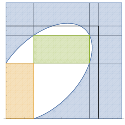
Figure 4: Values of $\displaystyle\rho$ which yield existence and non-existence results for $\displaystyle\left(\mathbb{B}^{2},g_{0}\right)$.

Proof of Theorem 1.3.

Let $\displaystyle u=(u_{1},u_{2})$ be a solution of (12). Since both components vanish on the boundary, for any $\displaystyle x\in\partial\mathbb{B}$ one has $\displaystyle\nabla u_{i}(x)=(\nabla u_{i}(x)\cdot\nu(x))\nu(x)=:\partial_{\nu}u_{i}(x)\nu(x)$ for both $\displaystyle i=1,2$.
Therefore, one can apply a standard Pohožaev identity:

$$\displaystyle\int_{\partial\mathbb{B}}\left((\partial_{\nu}u_{1})^{2}+\partial_{\nu}u_{1}\partial_{\nu}u_{2}+(\partial_{\nu}u_{2})^{2}\right)\mathrm{d}\sigma$$

$$\displaystyle= \displaystyle 2\int_{\partial\mathbb{B}}\left((\partial_{\nu}u_{1})^{2}-\frac{|\nabla u_{1}|^{2}}{2}+\partial_{\nu}u_{1}\partial_{\nu}u_{2}-\frac{\nabla u_{1}\cdot\nabla u_{2}}{2}+(\partial_{\nu}u_{2})^{2}-\frac{|\nabla u_{2}|^{2}}{2}\right)\mathrm{d}\sigma$$

$$\displaystyle= \displaystyle\int_{\mathbb{B}}\left(2(x\cdot\nabla u_{1}(x))\Delta u_{1}(x)+(x\cdot\nabla u_{1}(x))\Delta u_{2}(x)+(x\cdot\nabla u_{2}(x))\Delta u_{1}(x)+2(x\cdot\nabla u_{2}(x))\Delta u_{2}(x)\right)\mathrm{d}x$$

$$\displaystyle= \displaystyle-3\frac{\rho_{1}}{\int_{\mathbb{B}}|x|^{2\alpha_{1}}e^{u_{1}(x)}\mathrm{d}x}\int_{\mathbb{B}}(x\cdot\nabla u_{1}(x))|x|^{2\alpha_{1}}e^{u_{1}(x)}\mathrm{d}x-3\frac{\rho_{2}}{\int_{\mathbb{B}}|x|^{2\alpha_{2}}e^{u_{2}(x)}\mathrm{d}x}\int_{\mathbb{B}}(x\cdot\nabla u_{2}(x))|x|^{2\alpha_{2}}e^{u_{2}(x)}\mathrm{d}x$$

$$\displaystyle= \displaystyle 6\rho_{1}\frac{\int_{\partial\mathbb{B}}|\cdot|^{2\alpha_{1}}e^{u_{1}}\mathrm{d}\sigma}{\int_{\mathbb{B}}|x|^{2\alpha_{1}}e^{u_{1}(x)}\mathrm{d}x}+6(1+\alpha_{1})\rho_{1}+6\rho_{2}\frac{\int_{\partial\mathbb{B}}|\cdot|^{2\alpha_{1}}e^{u_{2}}\mathrm{d}\sigma}{\int_{\mathbb{B}}|x|^{2\alpha_{2}}e^{u_{2}(x)}\mathrm{d}x}+6(1+\alpha_{2})\rho_{2}.$$

For the boundary integral, we can perform an algebraic manipulation, use Hölder’s inequality and then integrate by parts:

$$\displaystyle\int_{\partial\mathbb{B}}\left((\partial_{\nu}u_{1})^{2}+\partial_{\nu}u_{1}\partial_{\nu}u_{2}+(\partial_{\nu}u_{2})^{2}\right)\mathrm{d}\sigma$$

$$\displaystyle= \displaystyle\int_{\partial\mathbb{B}}\left(\frac{1}{4}(\partial_{\nu}u_{1}+2\partial_{\nu}u_{2})^{2}+\frac{3}{4}(\partial_{\nu}u_{1})^{2}\right)\mathrm{d}\sigma$$

$$\displaystyle\geq \displaystyle\frac{1}{2\pi}\left(\frac{1}{4}\left(\int_{\partial\mathbb{B}}\partial_{\nu}u_{1}\mathrm{d}\sigma+2\int_{\partial\mathbb{B}}\partial_{\nu}u_{2}\mathrm{d}\sigma\right)^{2}+\frac{3}{4}\left(\int_{\partial\mathbb{B}}\partial_{\nu}u_{1}\mathrm{d}\sigma\right)^{2}\right)$$

$$\displaystyle= \displaystyle\frac{1}{2\pi}\left(\left(\int_{\partial\mathbb{B}}\partial_{\nu}u_{1}\mathrm{d}\sigma\right)^{2}+\left(\int_{\partial\mathbb{B}}\partial_{\nu}u_{1}\mathrm{d}\sigma\right)\left(\int_{\partial\mathbb{B}}\partial_{\nu}u_{2}\mathrm{d}\sigma\right)+\left(\int_{\partial\mathbb{B}}\partial_{\nu}u_{2}\mathrm{d}\sigma\right)^{2}\right)$$

$$\displaystyle= \displaystyle\frac{1}{2\pi}\left(\left(\int_{\mathbb{B}}\Delta u_{1}(x)\mathrm{d}x\right)^{2}+\left(\int_{\mathbb{B}}\Delta u_{1}(x)\mathrm{d}x\right)\left(\int_{\mathbb{B}}\Delta u_{2}(x)\mathrm{d}x\right)+\left(\int_{\mathbb{B}}\Delta u_{2}(x)\mathrm{d}x\right)^{2}\right)$$

$$\displaystyle= \displaystyle\frac{3}{2\pi}\left(\rho_{1}^{2}-\rho_{1}\rho_{2}+\rho_{2}^{2}\right).$$

Therefore, we get as a necessary condition for existence of solutions:

$$\displaystyle\rho_{1}^{2}-\rho_{1}\rho_{2}+\rho_{2}^{2} \displaystyle= \displaystyle 4\pi\left(\rho_{1}\frac{\int_{\partial\mathbb{B}}|\cdot|^{2\alpha_{1}}e^{u_{1}}\mathrm{d}\sigma}{\int_{\mathbb{B}}|x|^{2\alpha_{1}}e^{u_{1}(x)}\mathrm{d}x}+(1+\alpha_{1})\rho_{1}+\rho_{2}\frac{\int_{\partial\mathbb{B}}|\cdot|^{2\alpha_{1}}e^{u_{2}}\mathrm{d}\sigma}{\int_{\mathbb{B}}|x|^{2\alpha_{2}}e^{u_{2}(x)}\mathrm{d}x}+(1+\alpha_{2})\rho_{2}\right)$$

$$\displaystyle> \displaystyle 4\pi(1+\alpha_{1})\rho_{1}+4\pi(1+\alpha_{2})\rho_{2}.$$

This concludes the proof. ∎

Let us now consider the standard sphere $\displaystyle\left(\mathbb{S}^{2},g_{0}\right)$ with two antipodal singularities.

In Theorem 1.4 we perform a stereographic projection that transforms the solutions of (3) on $\displaystyle\mathbb{S}^{2}$ on entire solutions on the plane, and then we use a Pohožaev identity for the latter problem, getting necessary algebraic condition for the existence of solutions.
Such a Pohožaev identity yields an algebraic condition which is similar to the one which appears in Theorem 1.3. It can be deduced in the same way as was done in [16] for the scalar Liouville equation.

Theorem 7.1.

Let $\displaystyle H_{1},H_{2}\in L^{p}_{\mathrm{loc}}\left(\mathbb{R}^{2}\right)$ be such that, for suitable $\displaystyle a>0,\,b>-2,\,C>0$,

$$\frac{|x|^{a}}{C}\leq H_{i}(x)\leq C|x|^{b}\quad\forall\,x\in B_{1}(0)\setminus\{0\}\quad\quad\quad 0<H_{i}(x)\leq C|x|^{a}\quad\forall\,x\in\mathbb{R}^{2}\setminus B_{1}(0);$$

let $\displaystyle U=(U_{1},U_{2})$ be a solution of

$$\left\{\begin{array}[]{ll}-\Delta U_{1}=2H_{1}e^{U_{1}}-H_{2}e^{U_{2}}&\text{on }\mathbb{R}^{2}\\ -\Delta U_{2}=2H_{2}e^{U_{2}}-H_{1}e^{U_{1}}&\text{on }\mathbb{R}^{2}\\ \int_{\mathbb{R}^{2}}\left(|x|^{a}+|x|^{b}\right)e^{U_{1}(x)}\mathrm{d}x<+\infty\\ \int_{\mathbb{R}^{2}}\left(|x|^{a}+|x|^{b}\right)e^{U_{2}(x)}\mathrm{d}x<+\infty\end{array}\right.$$

and define

$$\rho_{i}:=\int_{\mathbb{R}^{2}}H_{i}(x)e^{U_{i}(x)}\mathrm{d}x,\quad\quad\quad,\tau_{i}:=\int_{\mathbb{R}^{2}}(x\cdot\nabla H_{i}(x))e^{U_{i}(x)}\mathrm{d}x,\quad\quad\quad i=1,2.$$

Then,

$$\rho_{1}^{2}-\rho_{1}\rho_{2}+\rho_{2}^{2}-4\pi\rho_{1}-4\pi\rho_{2}-2\pi\tau_{1}-2\pi\tau_{2}=0.$$

We get non-existence of solution for the parameter $\displaystyle\rho$ belonging to two or more regions of the positive quadrant. Such regions are colored in blue in Figure $\displaystyle 5$, whereas orange and green regions are the ones for which we have existence of solutions. The pictures show that non-existence phenomena may occur in each of the rectangles where the analysis of Theorem 1.1 gave no information. Using the notation of the theorem, these are the cases $\displaystyle(M_{1},M_{2},M_{3})\in\{(1,m,0),(m,1,0),(2,2,1)\}$.

We remark that Theorem 1.4 also applies to the case of $\displaystyle\alpha_{im}\geq 0$. This shows that the existence result in [6] cannot be extended if the hypothesis of positive genus of $\displaystyle\Sigma$ is removed.

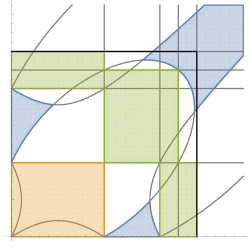
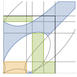
Figure 5: Values of $\displaystyle\rho$ which yield existence and non-existence results for $\displaystyle\left(\mathbb{S}^{2},g_{0}\right)$, in two different configurations of $\displaystyle\alpha_{11},\alpha_{12},\alpha_{21},\alpha_{22}$.

Proof of Theorem 1.4.

Let $\displaystyle u=(u_{1},u_{2})$ be a solution of

$$\left\{\begin{array}[]{l}-\Delta_{g_{0}}u_{1}=2\rho_{1}\left(\frac{e^{u_{1}}}{\int_{\mathbb{S}^{2}}e^{u_{1}}dV_{g_{0}}}-\frac{1}{4\pi}\right)-\rho_{2}\left(\frac{e^{u_{2}}}{\int_{\mathbb{S}^{2}}e^{u_{2}}dV_{g_{0}}}-\frac{1}{4\pi}\right)-4\pi\alpha_{11}\left(\delta_{p_{1}}-\frac{1}{4\pi}\right)-4\pi\alpha_{12}\left(\delta_{p_{2}}-\frac{1}{4\pi}\right)\\ -\Delta_{g_{0}}u_{2}=2\rho_{2}\left(\frac{e^{u_{2}}}{\int_{\mathbb{S}^{2}}e^{u_{2}}dV_{g_{0}}}-\frac{1}{4\pi}\right)-\rho_{1}\left(\frac{e^{u_{1}}}{\int_{\mathbb{S}^{2}}e^{u_{1}}dV_{g_{0}}}-\frac{1}{4\pi}\right)-4\pi\alpha_{22}\left(\delta_{p_{1}}-\frac{1}{4\pi}\right)-4\pi\alpha_{21}\left(\delta_{p_{2}}-\frac{1}{4\pi}\right)\end{array}\right.$$

and let $\displaystyle\Pi:\mathbb{S}^{2}\setminus\{p_{2}\}\to\mathbb{R}^{2}$ be the stereographic projection. Consider now, for $\displaystyle x\in\mathbb{R}^{2}$,

$$\left\{\begin{array}[]{l}U_{1}(x):=u_{1}\left(\Pi^{-1}(x)\right)+\log(4\rho_{1})-\log\int_{\mathbb{S}^{2}}e^{u_{1}}dV_{g_{0}}-2\alpha_{11}\log|x|+\left(\frac{\rho_{1}}{2\pi}-\frac{\rho_{2}}{4\pi}-\alpha_{11}-\alpha_{12}\right)\log\left(1+|x|^{2}\right)\\ U_{2}(x):=u_{2}\left(\Pi^{-1}(x)\right)+\log(4\rho_{2})-\log\int_{\mathbb{S}^{2}}e^{u_{2}}dV_{g_{0}}-2\alpha_{21}\log|x|+\left(\frac{\rho_{2}}{2\pi}-\frac{\rho_{1}}{4\pi}-\alpha_{21}-\alpha_{22}\right)\log\left(1+|x|^{2}\right)\end{array}\right..$$

$\displaystyle U=(U_{1},U_{2})$ solves

$$\left\{\begin{array}[]{l}-\Delta U_{1}=2H_{1}e^{U_{1}}-H_{2}e^{U_{2}}\\ -\Delta U_{2}=2H_{2}e^{U_{2}}-H_{1}e^{U_{1}}\\ \int_{\mathbb{R}^{2}}H_{1}(x)e^{U_{1}(x)}\mathrm{d}x=\rho_{1}\\ \int_{\mathbb{R}^{2}}H_{2}(x)e^{U_{2}(x)}\mathrm{d}x=\rho_{2}\end{array}\right.\quad\quad\quad\text{with}\quad\quad\quad\left\{\begin{array}[]{l}H_{1}(x):=\frac{|x|^{2\alpha_{11}}}{\left(1+|x|^{2}\right)^{2+\alpha_{11}+\alpha_{12}-\frac{\rho_{1}}{2\pi}+\frac{\rho_{2}}{4\pi}}}\\ H_{2}(x):=\frac{|x|^{2\alpha_{21}}}{\left(1+|x|^{2}\right)^{2+\alpha_{21}+\alpha_{22}-\frac{\rho_{2}}{2\pi}+\frac{\rho_{1}}{4\pi}}}\end{array}\right..$$

From Theorem 7.1, a necessary condition for existence of solutions is

$$\rho_{1}^{2}-\rho_{1}\rho_{2}+\rho_{2}^{2}-4\pi\rho_{1}-4\pi\rho_{2}-2\pi\tau_{1}-2\pi\tau_{2}=0.$$ (41)

with $\displaystyle\tau_{1},\tau_{2}$ as in the lemma. Moreover, by the definition of $\displaystyle H_{1},H_{2}$, we have

$$x\cdot\nabla H_{i}(x)=2\alpha_{i1}H_{i}(x)-2\left(2+\alpha_{i1}+\alpha_{i2}-\frac{\rho_{i}}{2\pi}+\frac{\rho_{3-i}}{4\pi}\right)\frac{|x|^{2}}{1+|x|^{2}}H_{i}(x)$$

for both $\displaystyle i$’s, hence we get

$$\tau_{i}=2\alpha_{i1}\rho_{i}-2\left(2+\alpha_{i1}+\alpha_{i2}-\frac{\rho_{i}}{2\pi}+\frac{\rho_{3-i}}{4\pi}\right)\tau^{\prime}_{i}\quad\quad\quad\text{with}\quad\quad\quad\tau^{\prime}_{i}:=\int_{\mathbb{R}^{2}}\frac{|x|^{2}}{1+|x|^{2}}H_{i}(x)\mathrm{d}x.$$

Therefore the necessary condition (41) becomes

$$\displaystyle\rho_{1}^{2}+\rho_{2}^{2}-\rho_{1}\rho_{2}-4\pi(1+\alpha_{11})\rho_{1}-4\pi(1+\alpha_{21})\rho_{2} \displaystyle+ \displaystyle 4\pi\left(2+\alpha_{11}+\alpha_{12}-\frac{\rho_{1}}{2\pi}+\frac{\rho_{2}}{4\pi}\right)\tau^{\prime}_{1}$$

$$\displaystyle+ \displaystyle 4\pi\left(2+\alpha_{21}+\alpha_{22}-\frac{\rho_{2}}{2\pi}+\frac{\rho_{1}}{4\pi}\right)\tau^{\prime}_{2}=0.$$

Using the straightforward inequalities $\displaystyle 0<\tau^{\prime}_{i}<\rho_{i}$ and discussing the cases $\displaystyle 2+\alpha_{i1}+\alpha_{i2}\lesseqqgtr\frac{\rho_{i}}{2\pi}-\frac{\rho_{3-i}}{4\pi}$, one can easily see by algebraic computation that (13) and their opposite inequalities are in contradiction with the aforementioned necessary condition.
Notice that if $\displaystyle\left\{\begin{array}[]{l}2+\alpha_{11}+\alpha_{12}=\frac{\rho_{1}}{2\pi}-\frac{\rho_{2}}{4\pi}\\ 2+\alpha_{21}+\alpha_{22}=\frac{\rho_{2}}{2\pi}-\frac{\rho_{1}}{4\pi}\end{array}\right.$, then (7.1) just becomes $\displaystyle\rho_{1}^{2}+\rho_{2}^{2}-\rho_{1}\rho_{2}-4\pi(1+\alpha_{11})\rho_{1}-4\pi(1+\alpha_{21})\rho_{2}=0$. Anyway, one can easily see that these two conditions are equivalent to having all equalities in (13); this is the reason why we need to assume at least one inequality to be strict. ∎

7.2 Proof of Theorems 1.5 and 1.6

We start by proving Theorem 1.5. We will argue by contradiction, following [11] (Theorem $\displaystyle 4.1$). Basically, we will assume that a solution exists for some $\displaystyle\alpha_{11}^{n},\alpha_{12}^{n}\underset{n\to+\infty}{\longrightarrow}-1$. We will consider such a sequence of solutions $\displaystyle u^{n}$, we will perform a blow-up analysis, following Theorem 2.1 and we will reach a contradiction.

Proof of Theorem 1.5.

Assume the thesis is false. Then, for some given $\displaystyle\underline{\alpha}_{1\widehat{1}},\underline{\alpha}_{2\widehat{1}},\rho\not\in\Gamma_{\underline{\alpha}_{1\widehat{1}},\underline{\alpha}_{2\widehat{1}}}$, there exist a sequence $\displaystyle(\alpha_{11}^{n},\alpha_{21}^{n})\underset{n\to+\infty}{\longrightarrow}(-1,-1)$ and a sequence $\displaystyle u^{n}=(u_{1}^{n},u_{2}^{n})$ of solutions of

$$\left\{\begin{array}[]{l}-\Delta u_{1}^{n}=2\rho_{1}\left(\frac{\widetilde{h}_{1}^{n}e^{u_{1}^{n}}}{\int_{\Sigma}\widetilde{h}_{1}^{n}e^{u_{1}^{n}}\mathrm{d}V_{g}}-1\right)-\rho_{2}\left(\frac{\widetilde{h}_{2}^{n}e^{u_{2}^{n}}}{\int_{\Sigma}\widetilde{h}_{2}^{n}e^{u_{2}^{n}}\mathrm{d}V_{g}}-1\right)\\ -\Delta u_{2}^{n}=2\rho_{2}\left(\frac{\widetilde{h}_{2}^{n}e^{u_{2}^{n}}}{\int_{\Sigma}\widetilde{h}_{2}^{n}e^{u_{2}^{n}}\mathrm{d}V_{g}}-1\right)-\rho_{1}\left(\frac{\widetilde{h}_{1}^{n}e^{u_{1}^{n}}}{\int_{\Sigma}\widetilde{h}_{1}^{n}e^{u_{1}^{n}}\mathrm{d}V_{g}}-1\right)\end{array}\right.,$$

with $\displaystyle\widetilde{h}_{1}^{n},\widetilde{h}_{2}^{n}$ such that $\displaystyle\widetilde{h}_{i}^{n}\sim d(\cdot,p_{1})^{2\alpha_{i1}^{n}}$. It is not restrictive to assume

$$\int_{\Sigma}\widetilde{h}_{1}^{n}e^{u_{1}^{n}}\mathrm{d}V_{g}=\int_{\Sigma}\widetilde{h}_{2}^{n}e^{u_{2}^{n}}\mathrm{d}V_{g}=1.$$

We would like to apply Theorem 2.1 to the sequence $\displaystyle u^{n}$. Anyway, since the coefficients $\displaystyle\alpha_{i1}^{n}$ are not bounded away from $\displaystyle-1$, we cannot use such a theorem on the whole $\displaystyle\Sigma$, but we have to remove a neighborhood of $\displaystyle p_{1}$. A first piece of information about blow-up is given by the following Lemma, inspired by [11], Lemma $\displaystyle 4.3$.∎

Lemma 7.2.

Let $\displaystyle\delta>0$ small be given and $\displaystyle u^{n}$ be as in the proof of Theorem 1.5. Then, $\displaystyle u_{1}^{n},u_{2}^{n}$ cannot be both uniformly bounded from below on $\displaystyle\partial B_{\delta}(p_{1})$.

Proof.

Assume by contradiction that $\displaystyle\inf_{\partial B_{\delta}(p_{1})}u_{i}^{n}\geq-C$ for both $\displaystyle i$’s and define $\displaystyle v^{n}:=\frac{2u_{1}^{n}+u_{2}^{n}}{3}$. Then

$$\left\{\begin{array}[]{ll}-\Delta v^{n}=\rho_{1}\left(\widetilde{h}_{1}^{n}e^{u_{1}^{n}}-1\right)\geq-\rho_{1}&\text{in }B_{\delta}(p_{1})\\ v^{n}\geq-C&\text{on }\partial B_{\delta}(p_{1})\end{array}\right..$$

By the maximum principle, $\displaystyle v^{n}\geq-C$ on $\displaystyle B_{\delta}(p_{1})$, therefore by the convexity of the exponential function we get the following contradiction:

$$\displaystyle+\infty \displaystyle\underset{n\to+\infty}{\longleftarrow} \displaystyle\int_{B_{\delta}(p_{1})}d(\cdot,p_{1})^{2\max\{\alpha_{11}^{n},\alpha_{21}^{n}\}}\mathrm{d}V_{g}$$

$$\displaystyle\leq \displaystyle C\int_{B_{\delta}(p_{1})}d(\cdot,p_{1})^{2\max\{\alpha_{11}^{n},\alpha_{21}^{n}\}}e^{v^{n}}\mathrm{d}V_{g}$$

$$\displaystyle\leq \displaystyle C\left(\frac{2}{3}\int_{B_{\delta}(p_{1})}d(\cdot,p_{1})^{2\max\{\alpha_{11}^{n},\alpha_{21}^{n}\}}e^{u_{1}^{n}}\mathrm{d}V_{g}+\frac{1}{3}\int_{B_{\delta}(p_{1})}d(\cdot,p_{1})^{2\max\{\alpha_{11}^{n},\alpha_{21}^{n}\}}e^{u_{2}^{n}}\mathrm{d}V_{g}\right)$$

$$\displaystyle\leq \displaystyle C\left(\int_{B_{\delta}(p_{1})}\widetilde{h}_{1}^{n}e^{u_{1}^{n}}\mathrm{d}V_{g}+\int_{B_{\delta}(p_{1})}\widetilde{h}_{2}^{n}e^{u_{2}^{n}}\mathrm{d}V_{g}\right)$$

$$\displaystyle\leq \displaystyle C.$$

This concludes the proof. ∎

Proof of Theorem 1.5, continued.

Let us apply Theorem 2.1 to $\displaystyle u^{n}$ on $\displaystyle\Omega:=\Sigma\setminus B_{\frac{\delta}{2}}(p_{1})$ for some given small $\displaystyle\delta>0$. By Lemma 7.2, boundedness from below cannot occur for both components, therefore we either have blow-up or (up to switching the indexes) $\displaystyle u_{1}^{n}\underset{n\to+\infty}{\longrightarrow}-\infty$ uniformly on $\displaystyle\Sigma\setminus B_{\delta}(p_{1})$. In other words,

$$\left.\rho_{1}\frac{\widetilde{h}_{1}^{n}e^{u_{1}^{n}}}{\int_{\Sigma}\widetilde{h}_{1}^{n}e^{u_{1}^{n}}\mathrm{d}V_{g}}\right\lfloor_{\Sigma\setminus B_{\delta}(p_{1})}\underset{n\to+\infty}{\rightharpoonup}\sum_{x\in\mathcal{S}}\sigma_{1}(x)\delta_{x}\quad\quad\left.\rho_{2}\frac{\widetilde{h}_{2}^{n}e^{u_{2}^{n}}}{\int_{\Sigma}\widetilde{h}_{2}^{n}e^{u_{2}^{n}}\mathrm{d}V_{g}}\right\lfloor_{\Sigma\setminus B_{\delta}(p_{1})}\underset{n\to+\infty}{\rightharpoonup}r_{2}+\sum_{x\in\mathcal{S}}\sigma_{2}(x)\delta_{x},$$

where we set $\displaystyle\mathcal{S}=\emptyset$ if blow up does not occur. Anyway, being $\displaystyle\delta$ arbitrary, a diagonal argument gives

$$\rho_{1}\frac{\widetilde{h}_{1}^{n}e^{u_{1}^{n}}}{\int_{\Sigma}\widetilde{h}_{1}^{n}e^{u_{1}^{n}}\mathrm{d}V_{g}}\underset{n\to+\infty}{\rightharpoonup}\sum_{x\in\mathcal{S}}\sigma_{1}(x)\delta_{x}+\sigma_{1}(p_{1})\delta_{p_{1}}\quad\quad\rho_{2}\frac{\widetilde{h}_{2}^{n}e^{u_{2}^{n}}}{\int_{\Sigma}\widetilde{h}_{2}^{n}e^{u_{2}^{n}}\mathrm{d}V_{g}}\underset{n\to+\infty}{\rightharpoonup}r_{2}+\sum_{x\in\mathcal{S}}\sigma_{2}(x)\delta_{x}+\sigma_{2}(p_{1})\delta_{p_{1}},$$

with $\displaystyle\sigma_{1}(p_{1})=\rho_{1}-\sum_{x\in\mathcal{S}}\sigma_{1}(x)$ and $\displaystyle\sigma_{2}(p_{1})=\rho_{2}-\sum_{x\in\mathcal{S}}\sigma_{2}(x)-\int_{\Sigma}r_{2}\mathrm{d}V_{g}$.
By a variation of the Pohožaev identity (see [28], Proposition $\displaystyle 3.1$ and [8], Lemma $\displaystyle 2.4$), we get

$$\sigma_{1}(p_{1})^{2}-\sigma_{1}(p_{1})\sigma_{2}(p_{1})+\sigma_{2}(p_{1})^{2}=0,$$

that is $\displaystyle\sigma_{1}(p)=\sigma_{2}(p)=0$. In particular, we get $\displaystyle\rho_{1}=\sum_{x\in\mathcal{S}}\sigma_{1}(x)$, which means either $\displaystyle\rho_{1}=0$ or $\displaystyle\rho\in\Gamma_{\underline{\alpha}_{1\widehat{1}},\underline{\alpha}_{2\widehat{1}}}$ This contradicts the assumptions and proves the theorem.∎

We conclude by proving Theorem 1.6. The argument is somehow similar: we assume, by contradiction, to have a solution satisfying all the hypotheses for $\displaystyle\alpha_{23}^{n}\underset{n\to+\infty}{\longrightarrow}-1$. Then, we perform a blow-up analysis and we rule out the last case using Theorem 1.4.

Proof of Theorem 1.6.

Assume by contradiction there exists a sequence $\displaystyle\alpha_{23}^{n}\underset{n\to+\infty}{\longrightarrow}-1$ such that (3) has a solution $\displaystyle u^{n}$ satisfying all the hypotheses of Theorem 1.6 and, w.l.o.g., $\displaystyle\int_{\Sigma}\widetilde{h}_{1}^{n}e^{u_{1}^{n}}\mathrm{d}V_{g}=\int_{\Sigma}\widetilde{h}_{2}^{n}e^{u_{2}^{n}}\mathrm{d}V_{g}=1$. In particular, since $\displaystyle 4\pi(1+\alpha_{2m})<\rho_{2}^{n}<4\pi(2+\alpha_{2m}+\alpha_{23}^{n})$ for $\displaystyle m=1,2$, then $\displaystyle\rho_{2}^{n}\underset{n\to+\infty}{\longrightarrow}4\pi(1+\alpha_{21})=4\pi(1+\alpha_{22})$.
As in the proof of Theorem 1.5, we must have $\displaystyle\inf_{B_{\delta}(p_{3})}u_{2}^{n}\underset{n\to+\infty}{\longrightarrow}-\infty$ for small $\displaystyle\delta$, because otherwise we would have

$$1\geq\int_{B_{\delta}(p_{3})}\widetilde{h}_{2}^{n}e^{u_{2}^{n}}\mathrm{d}V_{g}\underset{n\to+\infty}{\geq}C\int_{B_{\delta}(p_{3})}d(\cdot,p_{3})^{2\alpha_{23}^{n}}\mathrm{d}V_{g}\underset{n\to+\infty}{\longrightarrow}+\infty.$$

Unlike before, we cannot apply the maximum principle to get $\displaystyle\inf_{\partial B_{\delta}(p_{3})}u_{2}^{n}\underset{n\to+\infty}{\longrightarrow}-\infty$. Anyway, this could be ruled out by the following argument: if $\displaystyle u_{2}^{n}$ were uniformly bounded from below on $\displaystyle\partial B_{\delta}(p_{3})$ and $\displaystyle u_{2}^{n}(x^{n})\underset{n\to+\infty}{\longrightarrow}-\infty$ for some $\displaystyle x^{n}\underset{n\to+\infty}{\longrightarrow}x\in B_{\delta}(p_{3})$, then applying Theorem 2.1 we would get blow-up at $\displaystyle x$ of the first component alone, which would give $\displaystyle\rho_{1}\geq\sigma_{1}(x)\geq 4\pi$, in contradiction to the assumptions of the theorem. Therefore, $\displaystyle u_{2}^{n}$ must go to $\displaystyle-\infty$ uniformly on $\displaystyle\partial B_{\delta}(p_{3})$, which means, by Theorem 2.1, blow-up with $\displaystyle r_{2}\equiv 0$.
The assumption $\displaystyle\rho_{2}<4\pi$ implies that such blow-up must occur at a subset of $\displaystyle\{p_{1},p_{2},p_{3}\}$. Blow-up in $\displaystyle p_{3}$ is also excluded because, by standard blow-up analysis (one can argue for instance as in [36], Lemma $\displaystyle 9$) it would imply $\displaystyle\rho_{1}\geq\sigma_{1}(p_{3})\geq 4\pi$; therefore, we must have $\displaystyle\widetilde{h}_{2}e^{u_{2}^{n}}\underset{n\to+\infty}{\rightharpoonup}4\pi(1+\alpha_{2m})\delta_{p_{m}}$ for some $\displaystyle m=1,2$; since the role of $\displaystyle p_{1}$ and $\displaystyle p_{2}$ is interchangeable, we can assume $\displaystyle m=1$.
Let us now consider $\displaystyle u_{1}^{n}$: it cannot blow up at $\displaystyle p_{1}$, because $\displaystyle\rho_{1}<4\pi(2+\alpha_{11}+\alpha_{12})$, and it cannot even blow up at any other points: in fact, since $\displaystyle u_{2}^{n}$ only blows up at $\displaystyle p_{1}$, then by Theorem 2.1 we would get $\displaystyle\rho_{1}=\sum_{x\in\mathcal{S}}\sigma_{1}(x)$, again contradicting the assumptions. Therefore, $\displaystyle u_{1}^{n}$ must converge to some $\displaystyle u_{1}$, which solves (up to subtracting a suitable combination of Green’s functions)

$$-\Delta u_{1}=2\rho_{1}\left(\frac{e^{u_{1}}}{\int_{\mathbb{S}^{2}}e^{u_{1}}\mathrm{d}V_{g_{0}}}-\frac{1}{4\pi}\right)-4\pi(2+\alpha_{11}+\alpha_{21})\left(\delta_{p_{1}}-\frac{1}{4\pi}\right)-4\pi\alpha_{12}\left(\delta_{p_{2}}-\frac{1}{4\pi}\right).$$

By applying Theorem 1.4 with $\displaystyle\rho_{2}=0$, or equivalently Proposition $\displaystyle 5.8$ in [2], we see that the last equation is not solvable since $\displaystyle 4\pi(1+\alpha_{12})<\rho_{1}<4\pi(2+\alpha_{11}+\alpha_{21})$. This gives a contradictions and proves the theorem.∎

Notice that, by repeating the same argument, we can find similar non-existence results in the cases $\displaystyle(M_{1},M_{2},M_{3})=(2,2,1)$ and $\displaystyle(1,m,0)$, with one coefficient being very close to $\displaystyle-1$. In the case $\displaystyle(1,m,0)$, we can also drop the assumptions on $\displaystyle\Sigma$ to be a standard sphere with antipodal singularities.

References

- [1] D. Bartolucci, F. De Marchis, and A. Malchiodi. Supercritical conformal metrics on surfaces with conical singularities. Int. Math. Res. Not. IMRN, (24):5625–5643, 2011.
- [2] D. Bartolucci and A. Malchiodi. An improved geometric inequality via vanishing moments, with applications to singular Liouville equations. Comm. Math. Phys., 322(2):415–452, 2013.
- [3] D. Bartolucci and G. Tarantello. The Liouville equation with singular data: a concentration-compactness principle via a local representation formula. J. Differential Equations, 185(1):161–180, 2002.
- [4] L. Battaglia. Moser-Trudinger inequalities for singular Liouville systems. preprint, 2014.
- [5] L. Battaglia. Existence and multiplicity result for the singular Toda system. J. Math. Anal. Appl., 424(1):49–85, 2015.
- [6] L. Battaglia, A. Jevnikar, A. Malchiodi, and D. Ruiz. A general existence result for the Toda system on compact surfaces. Adv. Math., 285:937–979, 2015.
- [7] L. Battaglia and A. Malchiodi. A Moser-Trudinger inequality for the singular Toda system. Bull. Inst. Math. Acad. Sin. (N.S.), 9(1):1–23, 2014.
- [8] L. Battaglia and G. Mancini. A note on compactness properties of the singular Toda system. Atti Accad. Naz. Lincei Rend. Lincei Mat. Appl., 26(3):299–307, 2015.
- [9] J. Bolton and L. M. Woodward. Some geometrical aspects of the -dimensional Toda equations. In Geometry, topology and physics (Campinas, 1996), pages 69–81. de Gruyter, Berlin, 1997.
- [10] E. Calabi. Isometric imbedding of complex manifolds. Ann. of Math. (2), 58:1–23, 1953.
- [11] A. Carlotto. On the solvability of singular Liouville equations on compact surfaces of arbitrary genus. Trans. Amer. Math. Soc., 366(3):1237–1256, 2014.
- [12] A. Carlotto and A. Malchiodi. Weighted barycentric sets and singular Liouville equations on compact surfaces. J. Funct. Anal., 262(2):409–450, 2012.
- [13] S.-Y. A. Chang and P. C. Yang. Conformal deformation of metrics on . J. Differential Geom., 27(2):259–296, 1988.
- [14] C.-C. Chen and C.-S. Lin. Mean field equation of Liouville type with singular data: topological degree. Comm. Pure Appl. Math., Accepted for publication.
- [15] W. X. Chen. A Trüdinger inequality on surfaces with conical singularities. Proc. Amer. Math. Soc., 108(3):821–832, 1990.
- [16] W. X. Chen and C. Li. Prescribing Gaussian curvatures on surfaces with conical singularities. J. Geom. Anal., 1(4):359–372, 1991.
- [17] S. S. Chern and J. G. Wolfson. Harmonic maps of the two-sphere into a complex Grassmann manifold. II. Ann. of Math. (2), 125(2):301–335, 1987.
- [18] Z. Djadli and A. Malchiodi. Existence of conformal metrics with constant -curvature. Ann. of Math. (2), 168(3):813–858, 2008.
- [19] G. Dunne. Self-dual Chern-Simons Theories. Lecture notes in physics. New series m: Monographs. Springer, 1995.
- [20] L. Fontana. Sharp borderline Sobolev inequalities on compact Riemannian manifolds. Comment. Math. Helv., 68(3):415–454, 1993.
- [21] D. Gilbarg and N. S. Trudinger. Elliptic partial differential equations of second order. Classics in Mathematics. Springer-Verlag, Berlin, 2001. Reprint of the 1998 edition.
- [22] A. Hatcher. Algebraic topology. Cambridge University Press, Cambridge, 2002.
- [23] A. Jevnikar, S. Kallel, and A. Malchiodi. A topological join construction and the Toda system on compact surfaces of arbitrary genus. preprint, 2014.
- [24] J. Jost, C. Lin, and G. Wang. Analytic aspects of the Toda system. II. Bubbling behavior and existence of solutions. Comm. Pure Appl. Math., 59(4):526–558, 2006.
- [25] J. Jost and G. Wang. Analytic aspects of the Toda system. I. A Moser-Trudinger inequality. Comm. Pure Appl. Math., 54(11):1289–1319, 2001.
- [26] C. Lin, J. Wei, and W. Yang. Degree counting and shadow system for Toda systems: one bubbling. preprint.
- [27] C.-S. Lin, J. Wei, and C. Zhao. Asymptotic behavior of Toda system in a bounded domain. Manuscripta Math., 137(1-2):1–18, 2012.
- [28] C.-S. Lin, J.-c. Wei, and L. Zhang. Classification of blowup limits for singular Toda systems. Anal. PDE, 8(4):807–837, 2015.
- [29] M. Lucia. A deformation lemma with an application to a mean field equation. Topol. Methods Nonlinear Anal., 30(1):113–138, 2007.
- [30] M. Lucia and M. Nolasco. Chern-Simons vortex theory and Toda systems. J. Differential Equations, 184(2):443–474, 2002.
- [31] A. Malchiodi. Variational methods for singular Liouville equations. Atti Accad. Naz. Lincei Cl. Sci. Fis. Mat. Natur. Rend. Lincei (9) Mat. Appl., 21(4):349–358, 2010.
- [32] A. Malchiodi and C. B. Ndiaye. Some existence results for the Toda system on closed surfaces. Atti Accad. Naz. Lincei Cl. Sci. Fis. Mat. Natur. Rend. Lincei (9) Mat. Appl., 18(4):391–412, 2007.
- [33] A. Malchiodi and D. Ruiz. New improved Moser-Trudinger inequalities and singular Liouville equations on compact surfaces. Geom. Funct. Anal., 21(5):1196–1217, 2011.
- [34] A. Malchiodi and D. Ruiz. A variational analysis of the Toda system on compact surfaces. Comm. Pure Appl. Math., 66(3):332–371, 2013.
- [35] J. Moser. A sharp form of an inequality by N. Trudinger. Indiana Univ. Math. J., 20:1077–1092, 1970/71.
- [36] H. Ohtsuka and T. Suzuki. Blow-up analysis for Toda system. J. Differential Equations, 232(2):419–440, 2007.
- [37] M. Struwe. The existence of surfaces of constant mean curvature with free boundaries. Acta Math., 160(1-2):19–64, 1988.
- [38] G. Tarantello. Selfdual gauge field vortices. Progress in Nonlinear Differential Equations and their Applications, 72. Birkhäuser Boston Inc., Boston, MA, 2008. An analytical approach.
- [39] G. Tarantello. Analytical, geometrical and topological aspects of a class of mean field equations on surfaces. Discrete Contin. Dyn. Syst., 28(3):931–973, 2010.
- [40] M. Troyanov. Prescribing curvature on compact surfaces with conical singularities. Trans. Amer. Math. Soc., 324(2):793–821, 1991.
- [41] J. Wei and L. Zhang. In preparation.
- [42] Y. Yang. Solitons in field theory and nonlinear analysis. Springer Monographs in Mathematics. Springer-Verlag, New York, 2001.